the Creative Commons Attribution 4.0 License.
the Creative Commons Attribution 4.0 License.
 | 10 Sep 2021
Evaluating methods for debris-flow prediction based on rainfall in an Alpine catchment
Alexandre Badoux
Brian W. McArdell
Elena Leonarduzzi
Peter Molnar
The prediction of debris flows is relevant because this type of natural hazard can pose a threat to humans and infrastructure. Debris-flow (and landslide) early warning systems often rely on rainfall intensity–duration (ID) thresholds. Multiple competing methods exist for the determination of such ID thresholds but have not been objectively and thoroughly compared at multiple scales, and a validation and uncertainty assessment is often missing in their formulation. As a consequence, updating, interpreting, generalizing and comparing rainfall thresholds is challenging. Using a 17-year record of rainfall and 67 debris flows in a Swiss Alpine catchment (Illgraben), we determined ID thresholds and associated uncertainties as a function of record duration. Furthermore, we compared two methods for rainfall definition based on linear regression and/or true-skill-statistic maximization. The main difference between these approaches and the well-known frequentist method is that non-triggering rainfall events were also considered for obtaining ID-threshold parameters. Depending on the method applied, the ID-threshold parameters and their uncertainties differed significantly. We found that 25 debris flows are sufficient to constrain uncertainties in ID-threshold parameters to ±30 % for our study site. We further demonstrated the change in predictive performance of the two methods if a regional landslide data set with a regional rainfall product was used instead of a local one with local rainfall measurements. Hence, an important finding is that the ideal method for ID-threshold determination depends on the available landslide and rainfall data sets. Furthermore, for the local data set we tested if the ID-threshold performance can be increased by considering other rainfall properties (e.g. antecedent rainfall, maximum intensity) in a multivariate statistical learning algorithm based on decision trees (random forest). The highest predictive power was reached when the peak 30 min rainfall intensity was added to the ID variables, while no improvement was achieved by considering antecedent rainfall for debris-flow predictions in Illgraben. Although the increase in predictive performance with the random forest model over the classical ID threshold was small, such a framework could be valuable for future studies if more predictors are available from measured or modelled data.
- Article
(5825 KB) - Full-text XML
- BibTeX
- EndNote


Debris flows are a common geomorphic process and hazardous phenomenon in mountain regions. They move rapidly as a surging flow of saturated debris. In contrast to other mass movements, such as shallow landslides, debris flows follow an established flow path, along which they often entrain substantial amounts of sediment and water stored in the channel (Hungr et al., 2014; de Haas et al., 2020). In Switzerland, where this study is conducted, landslides and debris flows caused 74 fatal accidents between 1946 and 2015 (Badoux et al., 2016). Globally, debris flows cause about 165 fatalities per year on average, with most of them occurring in mountainous regions of developing countries (Dowling and Santi, 2014). Furthermore, debris flows have the potential to damage property, infrastructure, managed forests and agricultural land (Hilker et al., 2009). Therefore, the development of early warning systems (EWSs) for debris flows and other rapid gravitational mass movements, involving novel measurement techniques and models, is a priority in many countries (Stähli et al., 2015). EWSs often rely on rainfall thresholds (Guzzetti et al., 2020). The most common rainfall thresholds are drawn in the rainfall duration (D) and mean rainfall intensity (I, or cumulative rainfall) space, taking the form I = αD−β, which is a linear curve in logarithmic space (Caine, 1980).
In alpine settings, debris flows mostly develop following a shallow hillslope landslide caused by increased pore water pressure (e.g. Iverson, 1997). Another cause can be runoff, where sediment deposits in the channel are mobilized as a mass movement (Takahashi, 1978, 1981) or sediments are progressively bulked up (Fryxwell and Horberg, 1943; Johnson and Rodine, 1984; Tognacca, 1999; Gregoretti, 2000). Physically based models considering these mechanisms can be used to infer ID thresholds, leading to debris-flow initiation (e.g. Berti and Simoni, 2005; Berti et al., 2020; Tang et al., 2019). However, because such models require a large number of input data of high quality, empirically determined ID thresholds are still more common and are determined at the local, regional or global scale (e.g. Caine, 1980; Guzzetti et al., 2007; Coe et al., 2008; Badoux et al., 2009; Staley et al., 2013; Abancó et al., 2016; Bel et al., 2017).
A challenge in the use of ID thresholds is that there are multiple competing methods for their determination, which have not been objectively and thoroughly compared at multiple scales. Furthermore, ID thresholds are rarely validated (Segoni et al., 2018). Consequently, generalizing and updating ID thresholds is challenging, as is comparing between them to hypothesize about the possible site-related differences in geomorphology, lithology, terrain and soil properties that lead to a different response to rainfall forcing (Segoni et al., 2018). The sensitivities of ID thresholds have to be better understood and studied for such comparisons to be meaningful. Major uncertainties arise from various issues related to the quality of the rainfall record used. ID thresholds often rely on rainfall data from rain gauges, which can be located on the valley floor or in a neighbouring valley rather than in the immediate vicinity of the debris-flow initiation area. Studies in the Italian Alps have shown that in orographically complex areas, especially for short convective rainstorms, precipitation intensities can decay significantly (30 %–60 %) within short distances (5–10 km) from the centre of the rainfall cell (Marra et al., 2016). This may lead to underestimations of α by up to 70 % and is one reason for the high false alarm rate of ID thresholds (Nikolopoulos et al., 2014). Another factor causing ID-threshold underestimation is the coarse temporal resolution of the rainfall data. Landslide and debris-flow data sets going far back in time or relying on satellite-based estimates of rainfall can be strongly affected by a coarse temporal resolution. Especially if events are triggered by short-duration storms (minutes to hours), the event mean rainfall intensity is considerably underestimated when daily rainfall records are used. In a study with synthetic data, Marra (2019) showed that using daily data results in significant threshold underestimation. Gariano et al. (2020) confirmed this effect for a real case study in Italy. However, the accuracy of ID thresholds based on rainfall data with a sub-daily resolution can also be limited, for example if the exact timings of the debris flows or landslides are unknown (Leonarduzzi and Molnar, 2020). This is often the case, unless the area is closely monitored or damage was caused and immediately recognized. Therefore, in studies where the landslide timing is only imprecisely known and sub-daily rainfall data are used, the entire rainfall event or the rainfall until the highest intensity was reached is considered to be the triggering rainfall. This uncertainty in event timing has been shown to lead to inflated triggering rainfall amounts and subsequently to overestimated ID thresholds (Staley et al., 2013; Leonarduzzi and Molnar, 2020; Bel et al., 2017). Additional uncertainties stem from the discretization of the rainfall time series into rainfall events. Rainfall events are usually separated by a minimum inter-event time (MIT), a period that is intended to mark separate, independent rainfall periods (Dunkerley, 2008). For studies in debris-flow torrents, the MIT can range from 10 min (e.g. Coe et al., 2008) to 6 h (e.g. Deganutti et al., 2000) and is often chosen subjectively without a sensitivity analysis. Bel et al. (2017) combined different MIT values with uncertainty in the timing of debris-flow detection in a French torrent. The obtained uncertainty bounds in ID thresholds encompassed almost all ID thresholds previously published from other torrents. Despite their importance, uncertainties in ID curves are seldom used in prediction.
The inaccuracies in rainfall data used to establish ID thresholds are one source of uncertainty leading to the high false alarm rate. ID thresholds are also criticized for ignoring other information contained in the rainfall time series, such as peak intensities and antecedent rainfall. For debris flows, peak intensities at a high temporal resolution (≤ 10 min) have been shown to have an especially high predictive power (e.g. Abancó et al., 2016; Bel et al., 2017). Multivariate statistical methods, such as logistic regression, have been tested and applied to improve the prediction of post-wildfire debris flows in the USA (Cannon et al., 2010; Staley et al., 2017) and for debris flows in a French Alpine torrent (Bel et al., 2017). More advanced machine learning techniques are also becoming an attractive tool in the geosciences as the availability of both measured and modelled data increases, and the careful investigation of all possible physical interactions between the variables exceeds our capacities (Reichstein et al., 2019). For post-wildfire debris-flow prediction, machine learning algorithms have in fact been shown to outperform logistic regression models and ID thresholds in predictions (Kern et al., 2017; Nikolopoulos et al., 2018).
Here, we address two research questions. First, what is the uncertainty associated with estimation methods, debris-flow record duration and the hazard data set in ID-threshold parameters? By resampling the Illgraben debris-flow record using different time windows, we estimate the confidence bounds of the ID-threshold parameters. Furthermore, we compare the uncertainties of two methods that have been used recently for determining ID-threshold parameters (e.g. Leonarduzzi et al., 2017; Leonarduzzi and Molnar, 2020; Nikolopoulos et al., 2018). These methods use linear regression and/or the true skill statistic to determine the ID-threshold parameters α and β. The differences in these methods are evaluated for both a local debris-flow inventory with local rainfall measurements and a regional landslide and debris-flow inventory with gridded rainfall information. Second, how do traditional ID-threshold-curve methods compare with machine learning algorithms? We extend the analysis of debris-flow prediction with additional rainfall event attributes in a random forest algorithm (Breiman, 2001), test the predictive skill, and discuss the pros and cons of the multivariate approach for local debris-flow detection based on different rainfall event properties (e.g. peak rainfall intensity, number of lightning events) and other seasonal proxies, for example those related to sediment recharge.
Illgraben is a north-facing catchment located in the Rhône valley in the Swiss canton of Valais (Fig. 1). It consists of two subcatchments: the eastern Illbach (4.15 km2) is hydrologically and geomorphologically disconnected, while the western Illgraben (4.83 km2) produces on average four to five debris flows a year. The Illgraben subcatchment has a maximum elevation of 2645 m a.s.l. just below the summit of the Illhorn mountain. In this region, the main Rhône–Simplon fault line changes its orientation, resulting in numerous smaller faults in highly fractured bedrock and affecting the Illgraben catchment (McArdell and Sartori, 2021). The main sediment source area is a highly active hillslope underlain by quartzite bedrock, ranging from 1250 to 2370 m a.s.l. and with slopes of up to 80°, where frequent landslides occur and deposit sediments in the trunk channel (Bennett et al., 2012; Berger et al., 2011). The main debris-flow channel starts just below this hillslope and is 5.2 km long. The first half is characterized by a mean slope of 16 % until the fan apex at 886 m a.s.l. (Badoux et al., 2009). The second half is flatter (10 %) and confined by check dams, before it joins the Rhône river at 605 m a.s.l.
In 1961 a large rock avalanche on the northern slope provided abundant sediment and increased the debris-flow frequency in the following years (Hürlimann et al., 2003). However, since then this part of the catchment has produced sediment at much lower rates than the main source area (Schlunegger et al., 2009). The rock avalanche prompted the construction of 30 concrete check dams to stabilize the channel, with the most upstream one being 48 m tall (Lichtenhahn, 1971). This upstream check dam was effective in stabilizing the toe of the rock avalanche deposit and reducing the number of debris-flow events in subsequent years (Hürlimann et al., 2003).
Since 2000 the Swiss Federal Institute for Forest, Snow and Landscape Research WSL has been operating an observation network in the Illgraben catchment (Fig. 1), including rain gauges (added in 2001), geophones, depth sensors and a force plate (Rickenmann et al., 2001; Hürlimann et al., 2003; McArdell et al., 2007; McArdell, 2016). In this study, we used the data from rain gauge 1 and a debris-flow inventory including events up to the year 2017 (McArdell and Hirschberg, 2020). The other two rain gauges are not ideal for this study because rain gauge 2 has changed location during the study period and rain gauge 3 is sheltered by trees. Rain gauge 1 is suitable here because it is close to the debris-flow initiation area and has been measuring consistently.
Illgraben has an alarm system that operates independently from the debris-flow observation station. It serves the village of Susten and the Pletschen subdivision on the eastern side of the fan and protects the people visiting the Pfynwald nature park on the western side. Furthermore, hiking trails and sports fields close to the riparian zone make the fan a vulnerable area. Geophones mounted on check dams detect debris flows and activate alert lights and acoustic signals downstream in the riparian zone. After an initial phase of testing and optimization by WSL (see Badoux et al., 2009), the alarm system is now operated by the local municipality in cooperation with an engineering company.
The mean annual precipitation at mean catchment elevation (1600 m a.s.l.) computed for the time period 1981–2010 was 900 mm yr−1 (Hydrological Atlas of Switzerland, 2015), and the mean annual temperature for the same period was 5.9 °C (Hirschberg et al., 2021). Debris flows generally occur from May to October. Although climate change scenarios project longer debris-flow seasons in the future (Hirschberg et al., 2021) and recently debris flows have also been recorded in April (2020) and December (2018), most debris flows occur in response to convective rainstorms between June and August. Snowmelt can add considerable amounts of liquid water to the debris in other places (e.g. Mostbauer et al., 2018) but has never been observed to be the sole debris-flow trigger in Illgraben, although it likely affects the antecedent conditions in spring. Debris flows overflowing the banks are only expected in the case of the failure of a landslide-generated dam, if there is levee failing or breaching, or if the channel conveyance capacity is reduced. Such a large debris flow was only observed after the failure of the dam formed by the 1961 rock avalanche (Badoux et al., 2009).
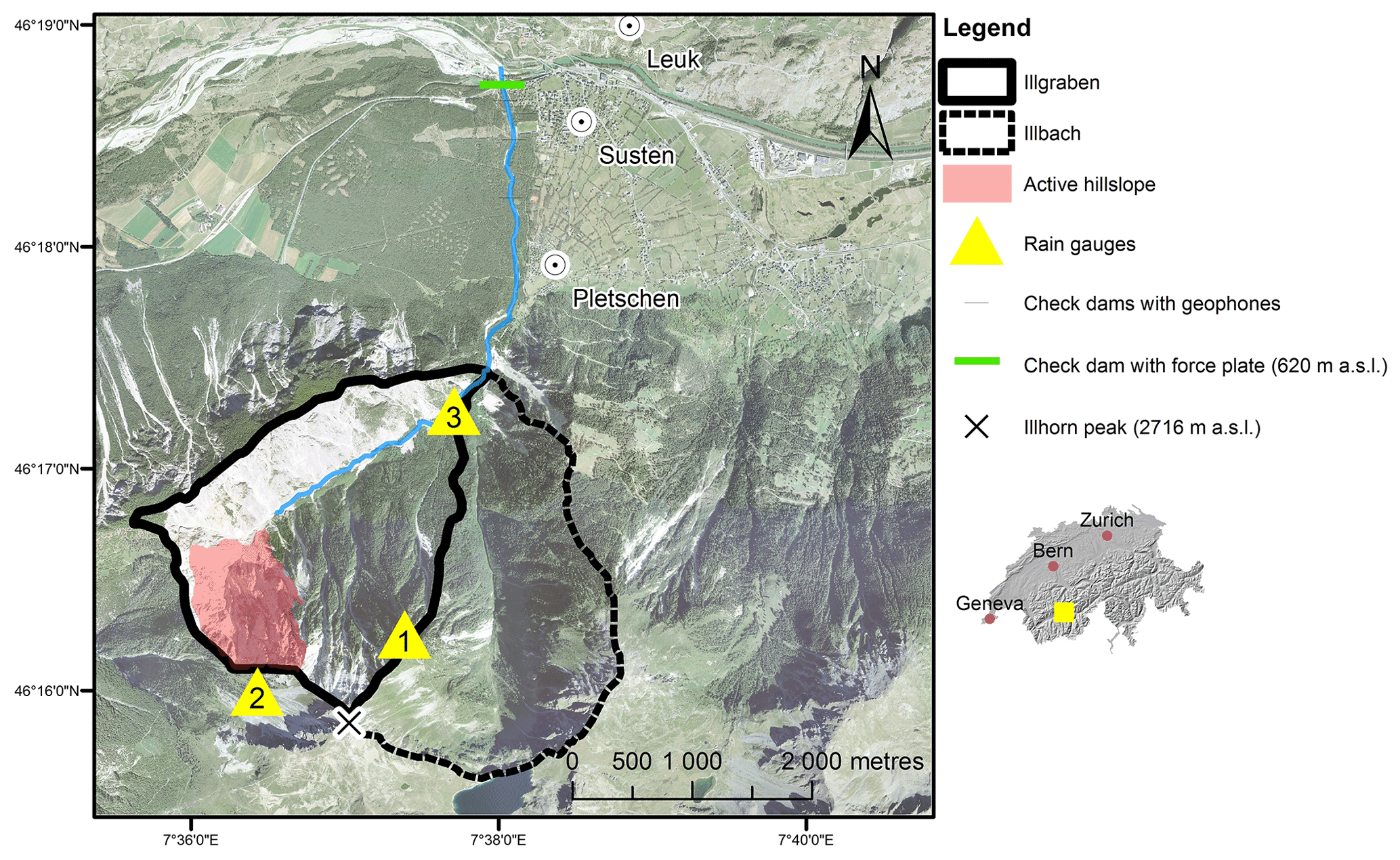
Figure 1Aerial view of the Illgraben study site (Federal Office of Topography) with the debris-flow observation station. Most sediments are generated on the active hillslope. Debris flows mostly initiate in the channel below this slope and are identified with geophones mounted to the check dams downstream. Volumes are calculated based on data collected at the location of the force plate. Data from rain gauge 1 were used in this study to characterize rainfall events.
3.1 Data
The timing and volume of debris flows were derived from the local observation system and are reported in McArdell and Hirschberg (2020). The debris-flow data set contains 75 entries from the years 2000 to 2017, with 1–8 debris flows occurring every year and bulk volumes ranging from 2000 to over 100 000 m3 (median 25 000 m3). The debris-flow mean bulk density was typically 1800–2200 kg m−3 (Schlunegger et al., 2009). Because the local rain gauges (Fig. 1) were installed in June 2001, only 67 of these debris flows overlap with the rainfall record and were used in this study. The local rain gauge is a 0.2 mm resolution tipping bucket with a 10 min sampling rate. It is not heated, and therefore only measurements in the period from May to October are considered, which coincides well with the debris-flow season. During this period, 480 mm of rainfall is measured annually on average, corresponding to about half of the total annual precipitation. The majority of debris flows are triggered by events with cumulative rainfall exceeding 5 mm. Although this amount is exceeded by about 30 storms each year, only 4.2 debris flows are triggered annually on average.
Temperature data were provided by the Swiss Federal Office of Meteorology and Climatology (MeteoSwiss) from the Montana meteorological station, located about 11 km northwest of the study area. Although the local rain gauges measure temperature, the sensors are not properly shielded, and the measurements are therefore unreliable. The measurements were interpolated using local lapse rates to account for the difference in elevation of about 200 m, as described in Hirschberg et al. (2021). The 10 min total of recorded lightning strikes at a distance of 3–30 km was also derived from the Montana station and used as a secondary variable for the convective character of storms (Gaál et al., 2014) in the machine learning algorithm. The local predictive power of debris flows in Illgraben was also compared with a regional prediction of slope failure using a regional data set on shallow landslides in Switzerland including associated rainfall events (Leonarduzzi et al., 2017). It is based on a gridded daily rainfall product (RhiresD) and the Swiss flood and landslide damage database of WSL (Hilker et al., 2009). RhiresD consists of a 1 km × 1 km gridded product of daily precipitation sums obtained by interpolation of rain gauges (ca. 420), accounting for local climatology and precipitation–topography relationships (Frei and Schär, 1998). The regional data set consists of 2137 landslides which occurred in Switzerland between 1972 and 2018 and for which damage was reported. Only the data from 2001 to 2017 were used here to be consistent with the local data set.
3.2 Performance statistics for debris-flow prediction
Confusion matrices and receiver operating characteristic (ROC) curves were used to compare models and optimize thresholds for debris flow triggering (Fawcett, 2006). A confusion matrix can be computed for any binary classifier by counting the true positives (TPs), false negatives (FNs), true negatives (TNs) and false positives (FPs). Various performance statistics can be calculated from the confusion matrix. The most common measures in debris-flow and landslide forecasting are the following (e.g. Staley et al., 2013; Gariano et al., 2015; Leonarduzzi et al., 2017; Leonarduzzi and Molnar, 2020; Mirus et al., 2018):
In the literature, the TSS is also referred to as the Peirce skill score (Peirce, 1884), Youden's index (Youden, 1950), or the Hanssen and Kuipers discriminant (Hanssen and Kuipers, 1965). The benefit of using the specificity over the false positive rate (FPR = FP(FP + TN)) is that in a perfect model TSS, sensitivity and specificity all equal 1. As noted by others (e.g. Leonarduzzi et al., 2017; Postance et al., 2018; Mirus et al., 2018), optimizing the TS leads to more conservative (higher) thresholds, while optimizing the TSS yields more balanced rainfall thresholds. The choice of score used in practice is therefore the user's decision. In this study, the TSS was optimized to calibrate thresholds and to compare classifiers, mainly because it is less sensitive to data sets with unbalanced class prevalence. In particular, the TSS was used in the following analyses:
-
in the determination of thresholds for single predictors (Sect. 3.3)
-
in the determination of the ID-threshold parameters (Sect. 3.4)
-
in the determination of probability thresholds from the random forest classifier (Sect. 3.5)
-
in the comparison of these predictive models.
Another metric for predictive model comparison is the area under the ROC curve (AUC). To estimate the AUC, SE and 1 − SP are calculated and plotted for all possible threshold values. AUC equals 1 if there is a threshold that can perfectly separate triggering and non-triggering events. A model with an AUC of 0.5 has no predictive power.
Table 1List of models and single predictors evaluated on their predictive performance for debris flow triggering. Data source “Illgraben” refers to the local rain gauge, “Montana” to the MeteoSwiss weather station located 11 km from the catchment and “Debris flows” to the Illgraben debris-flow data set.
3.3 Rainfall event definition and other properties
The precipitation time series was discretized into rainfall events, which were separated by a minimum inter-event time (MIT). Rainfall events were considered independent if no rainfall was recorded during this time. For triggering events, the end of the rainfall event was set either to the day of the event (for the regional data set) or to the 10 min instance before the event was recorded (for the local data set). This procedure avoids threshold overestimation (Staley et al., 2013; Leonarduzzi et al., 2017). For the regional data set we defined MIT as 1 d as in Leonarduzzi and Molnar (2020). This definition of events overestimates event duration and underestimates mean intensity compared to hourly data but compensates for this by longer and more dense records (see Leonarduzzi and Molnar, 2020). For rainfall records with a sub-daily resolution, MIT is often chosen subjectively and varies between 10 min at Chalk Cliffs (USA) and 6 h at Moscardo (Italy) for local debris-flow analyses (Coe et al., 2008; Deganutti et al., 2000). In Switzerland, an MIT of 2–3 h has been shown to be appropriate for the separation of thunderstorms (Gaál et al., 2014) and storms initiating bedload transport in an Alpine watershed (Badoux et al., 2012). However, as the subjectivity in the rainfall event definition complicates the comparison of rainfall thresholds, we followed the suggestion of Bel et al. (2017) to choose MIT for the local data set as the duration where the number of rainfall events stabilizes. In this process, the sensitivity of rainfall threshold performance scores to the choice of MIT was also evaluated (Fig. 2a). The measures SE, SP and TSS from fitting ID curves were found to decrease with increasing MIT as the number of events drops. However, in absolute terms, the number of false alarms is higher at a short MIT because of the large total number of rainfall events, and this is also reflected in the TS statistic. At MIT = 3 h, the number of rainfall events stabilizes. This is seen in the stable TS, meaning that there are no additional false alarms. The shape parameter of the ID threshold (β) reduces its increasing trend at the same MIT (Fig. 2b). The scale parameter (α) increases because the rainfall events become longer with increasing MIT, and therefore the rainfall amounts increase. Consequently, MIT = 3 h was used throughout this study, and it was confirmed that in the Alps an MIT of 2–3 h is an appropriate time period for separating rainfall into independent events for various applications, as found in independent studies by Badoux et al. (2012), Gaál et al. (2014) and Bel et al. (2017). Nevertheless, a suitable MIT should be objectively tested for each study site if possible.
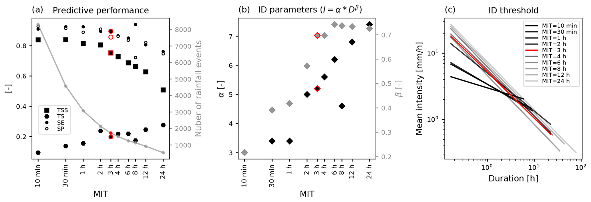
Figure 2ID thresholds and their predictive performance statistics as a function of the rainfall event definition (minimum inter-event time, MIT). (a) Analysis of the true skill statistic (TSS), threat score (TS), sensitivity (SE) and specificity (SP) as a function of MIT. The number of rainfall events also varies with MIT and is shown in grey. (b) Analysis of ID-threshold parameters as a function of MIT. (c) Visualization of ID thresholds for different values of MIT. An MIT of 3 h (red) was chosen for this study (see text).
Once MIT was defined, other rainfall event properties were extracted in addition to the duration and mean intensity (Table 1, single predictors). Multiple maximum rainfall intensities were computed over periods of 10 min to 2 h. Antecedent rainfall was defined as cumulative rainfall prior to the rainfall event and computed for a range of periods from 1 to 90 d prior to the rainfall event. These event properties can be computed from any rainfall time series and are important for the soil moisture saturation and the likelihood of runoff formation in response to rainfall.
Furthermore, event properties related to air temperature were added. The daily mean, minimum and maximum temperature was computed for the day of each rainfall event. If an event spanned several days, the day the event started was considered. In the case of low temperatures, it could be snowing in the higher parts of the catchment, reducing the amount of liquid water contributing to subsequent runoff. In this case, the rain gauge can possibly not be trusted because it is not heated. However, most debris flows occur in summer, when solid precipitation is rare even in the higher parts of the basin. As an indicator of convective rainfall, the daily temperature span and the number of lightning strikes were added. To account for seasonality effects, the day of year and the month of each event were included. As proxies for sediment availability, the time elapsed since the last debris flow was added and the number of freezing days of the current hydrological year (November–October) was computed from the temperature time series. The aim of the latter was to account for sediment recharge related to frost-weathering processes (Hirschberg et al., 2021).
3.4 Rainfall intensity–duration (ID) thresholds
ID thresholds are defined as I = αD−β (Caine, 1980). In the log–log space this relation becomes linear, where the scale parameter α defines the intercept of the threshold line and the shape parameter β its slope. The best way to determine the scale (α) and shape (β) parameters of rainfall ID curves and their uncertainties is the subject of ongoing discussion. Brunetti et al. (2010) presented a statistical approach (frequentist method) involving estimating β with a linear regression (in logarithmic space) fitted to all triggering rainfall events and decreasing α by an amount which is equal to the distance of the median residual to a chosen lower percentile. While this method is objective and, when applied as an EWS, makes it possible to control the hit rate, it neglects the information from the non-triggering rainfall events and thus does not consider the false positive rate. Lately, confusion matrices and ROCs (see Sect. 3.2) have been used as objective measures to assess the predictive performance of ID thresholds and also as an alternative way to determine α and β.
For the ID thresholds computed here, sensitivity (Eq. 1) and specificity (Eq. 2) were calculated. The threshold performance was then evaluated in terms of the TSS (Eq. 3). Two approaches were applied to optimize the ID-threshold parameters. In the first approach, as in the frequentist method, β is determined in the log–log space with a linear least-squares approximation of the debris-flow-triggering ID pairs. In a next step, α is tuned to maximize the TSS. This method is called LR&TSS hereafter. In the second approach, the scale parameter α and the shape parameter β are simultaneously tuned to maximize the TSS. This approach is hereafter referred to as TSS&TSS (Table 1, models). The fundamental difference in these two approaches is that LR&TSS only relies on triggering rainfall events to define β, while TSS&TSS considers both triggering and non-triggering rainfall events. Hence, different values and sensitivities for β can be expected for these two approaches depending on for example the number of triggering rainfall events and the ratio of triggering to non-triggering rainfall events.
To test the uncertainty of these two methods associated with the record duration, resampled (bootstrapped; James et al., 2013a) time series of rainfall and debris-flow/landslide events from 1 to 30 years were produced. Thus, only entire years were resampled to avoid breaking up any natural intra-annual patterns. One sampled year consisted of all debris-flow-triggering/landslide-triggering and non-triggering rainfall events. For example, for a record duration of 5 years, a sample consists of 5 years of measurement. Each year of measurement was drawn from the full 17-year observation period with replacement. This means that a specific year could occur multiple times in one 5-year sample. The multiple occurrence of the same year in a sample is fundamental to the uncertainty assessment and is of course more likely for longer than for shorter record durations. For each record duration, 100 samples were obtained by following this procedure, e.g. 100 samples with a record duration of 5 years. Finally, the bias in ID-threshold parameters was estimated for each sample. The bias was defined as the relative deviation of estimates of α and β from the corresponding reference values, i.e. the ones calculated from the original complete (17-year) record using LR&TSS and TSS&TSS.
3.5 Random forests for debris-flow prediction
Much of the information contained in the rainfall time series, such as antecedent rainfall and peak intensity, is lost when discretized into events and characterized only by mean rainfall intensity and duration. As an alternative, random forests (RFs, Breiman, 2001) were used to include more rainfall event properties (Table 1) for the classification of rainfall events into debris flow triggering and non-triggering. Random forests are based on a statistical learning algorithm that uses an ensemble of decision trees. Each of these trees is trained with a subset of the predictor variables in the training data set. This procedure (also called bagging) is fundamental to the algorithm because it decreases the correlation among the trees and makes random forests suitable for capturing complex interactions and structures in the data. For detailed information, the reader is referred to Breiman (2001) and James et al. (2013b). The scikit-learn module in Python was used to develop an RF classifier (Pedregosa et al., 2011).
For the prediction of debris flows, logistic regression models have been used extensively in regional post-fire debris-flow studies to account for rainfall threshold variability due to spatial differences in the slope and burned area (e.g. Cannon et al., 2010; Staley et al., 2017). Moreover, Bel et al. (2017) showed, for a French debris-flow torrent, that when ID thresholds were used in conjunction with a logistic regression model including variables for peak rainfall intensity, antecedent rainfall conditions and the number of days since winter, the number of false alarms could be reduced. RFs were used instead in the present study because of their ability to consider multiple predictor variables with non-linear relationships and correlating predictors. To our knowledge, the predictive power of RFs has not yet been tested for local debris-flow or landslide predictions. Nikolopoulos et al. (2018) used RFs for regional post-fire debris-flow predictions in the western United States and showed that RFs improved debris-flow predictions when a variable representing the location was added.
Here, four RF models – with the number of predictor variables ranging from 2 to 26 – were tested, with the first being the equivalent of the traditional ID threshold (RF_ID, Table 1). The model output included the probability of being debris flow triggering for every rainfall event. The probability threshold for classification had to be tuned because the threshold-optimizing TSS is likely not 50 % but rather somewhat smaller (Nikolopoulos et al., 2018). The predictive performance was then compared with the ID threshold obtained as described in Sect. 3.4 and with all single predictors (Table 1).
4.1 Debris-flow ID thresholds and their seasonality
In the study period from 2001 to 2017, 21 debris flows were triggered in spring and early summer (May and June, with the local influence of snowmelt), 38 in summer (July and August), and 8 in autumn (September and October) (Fig. 3). The monthly inter-annual variability was especially high in July, when between 0 and 6 debris flows occurred. This was also the month with the most extreme 30 min rainfall due to convective storms. The debris-flow activity dropped considerably in autumn, when the monthly rainfall also reduced by about 50 %. Such seasonality is typical of Alpine debris-flow torrents (e.g. Schneuwly-Bollschweiler and Stoffel, 2012; Bel et al., 2017). In spring, snowmelt generates additional runoff and saturates the debris, which may lower the rainfall threshold for debris-flow initiation. This likely played a role in the events which were triggered at low rainfall amounts (30 min duration) before mid-June. There were also some lower-intensity events in July and August which still triggered debris flows. However, at this time of the year, inaccurate rainfall measurements and high spatial variability during convective storms are a more likely explanation. The rainfall event with the highest peak 30 min rainfall intensity that did not trigger a debris flow was in October, possibly indicating sediment supply-limited conditions.
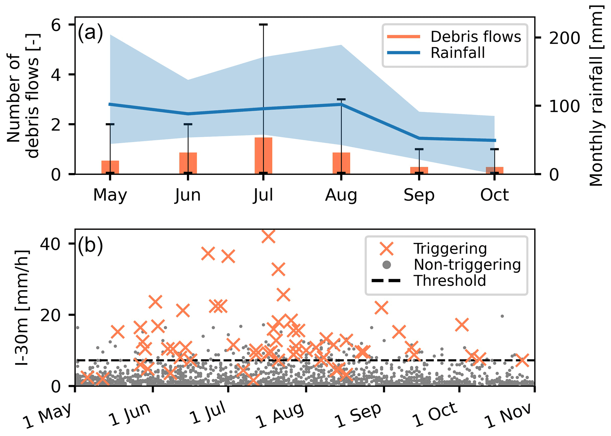
Figure 3(a) Mean number of debris flows per month (orange bars) and mean monthly rainfall (blue line) in the Illgraben catchment. The thin error bars (black) and the shaded area (blue) show the inter-annual variability, i.e. the observed minimum and maximum in each month between 2001 and 2017. (b) Peak 30 min rainfall intensity in debris-flow-triggering and non-triggering rainfall events. The threshold (7.2 mm h−1) was determined by optimizing the TSS (0.75).
Debris-flow-triggering threshold curves in Illgraben showed the typical negative power-law relationship between mean intensity and duration (Fig. 4). Debris flows occurred mostly during high rainfall intensities. However, triggering and non-triggering events could not be separated perfectly. There were a few outliers at very short (<1 h) and very long (>16 h) rainfall durations, which were triggered by comparably little rainfall. ID thresholds were computed with two methods (TSS&TSS and LR&TSS) for the entire data set and for individual seasons (Fig. 4). The scale parameter α had values between 2.6 and 7.3, with lower values for TSS&TSS (2.6–5.4) and higher values for LR&TSS (5.2–7.3). The shape parameter β was consistently smaller for TSS&TSS (0.26–0.93) than for LR&TSS (0.52–0.94) and varied considerably between the seasons. These parameter ranges largely comprise values reported for other debris-flow torrents (Bel et al., 2017). Only in spring were the two thresholds practically identical (Fig. 4b). For the entire data set, this resulted in the median TSS&TSS threshold being lower for short durations (≤ 4.5 h) and higher for long durations. The LR&TSS threshold was very similar to a curve defined earlier for Illgraben, with α=5.4 and β=0.79 (McArdell and Badoux, 2007), although in that case α was set to detect all triggering events. If the same procedure had been used for the data set used here, the ID threshold would also have been lower.

Figure 4ID thresholds for the Illgraben catchment computed with two methods. (a) ID thresholds for the entire data set. For the 67 triggering events, the 14 d antecedent rainfall (blue colour) and the (relative) bulk volume (marker size) of the debris flows are also shown. (b–d) ID thresholds for each season, where the lines are the thresholds computed using TSS&TSS (black) and LR&TSS (grey). The marker size indicates the total event rainfall.
The seasonal ID thresholds differed, but direct comparison is difficult because of differences in the number of events (Fig. 4b–c). In autumn, it is clearer than in other seasons that only the highest intensities for a given duration triggered debris flows. This may be due to (a) rainfall measurements being more representative and accurate for the initiation area than in summer when more convective events take place; (b) sediment availability being exhausted at the end of the debris-flow season (Berger et al., 2011; Bennett et al., 2014); or (c) grain size coarsening throughout the wet season, increasing the hydraulic conductivity in the channel bed and therefore also the rainfall threshold that must be exceeded to generate runoff (Domènech et al., 2019). As a consequence, the false alarm rate was lower in autumn than in other seasons.
For longer durations, larger rainfall amounts are required for debris flow triggering (Fig. 4b–d), and this reflects the balance of infiltration, storage and drainage of water. However, for short and long rainfall durations, ID pairs fail to plausibly describe the hydrological processes leading to landslide initiation (Bogaard and Greco, 2018). Here it was not clear if this was also the reason for the outliers triggered by lower mean rainfall intensities. There were two debris flows in summer at rainfall durations of 10 and 30 min which were triggered by significantly lower mean rainfall intensities than the other debris-flow events associated with these durations. One possible reason for this is that rain gauges, although close to the initiation area (∼ 1 km), are prone to not capturing peak intensities, especially of convective storms, even at short distances (Nikolopoulos et al., 2014; Marra et al., 2016). These two events were, however, also characterized by high antecedent rainfall, which could have lowered the triggering threshold. In spring, three events were triggered at low mean rainfall intensities (<1 mm h−1) and after more than 16 h. It could be that the MIT parameter does not separate rainfall events accurately in these cases; that the rainfall threshold was lower due to snowmelt; that there were errors in the rainfall data; or simply that these debris flows were triggered by mechanisms other than rainfall excess, such as the breaching of a small landslide dam.
Debris flows occur in a wide range of 14 d antecedent rainfall conditions, with many events occurring with very low values for this variable (Fig. 4a). Antecedent rainfall does not appear to be a significant precondition for debris flow triggering in the Illgraben catchment. This has also been observed at other alpine locations (e.g. Abancó et al., 2016). Here, the debris-flow magnitudes were not affected by the intensity of the triggering rainfall, which is consistent with other studies (Hirschberg et al., 2019; Pastorello et al., 2018). However, the magnitudes were affected by the amount of antecedent rainfall. Higher antecedent rainfall amounts lead to a higher degree of pore saturation along the entire channel bed. Although antecedent rainfall may also contribute to lateral flow on the hillslopes (e.g. Papa et al., 2013), the steep hillslopes in Illgraben and the timescale of 14 d give us confidence that this antecedent rainfall mainly affects the channel bed. In this case, sediment entrainment experiences a positive feedback from increased pore water pressure as the debris-flow surge passes by, increasing the debris-flow volume (Iverson et al., 2011; McCoy et al., 2012; Hirschberg et al., 2019).
4.2 Sensitivity of ID thresholds to record duration and identification method
Illgraben ID thresholds where the ID-threshold parameters are jointly tuned to optimize the TSS (TSS&TSS) have slightly larger TSS values compared with ID thresholds with parameters estimated by first fitting β to the triggering events and then tuning α to optimize the TSS (LR&TSS) (Fig. 5d). However, this increase in the TSS is accompanied by higher uncertainties, measured as the 10th to 90th percentile range, in both α and β biases (Fig. 5b, c). TSS&TSS thresholds are significantly lower than LR&TSS thresholds for short durations (<4.5 h) and higher for long durations (Fig. 5e).
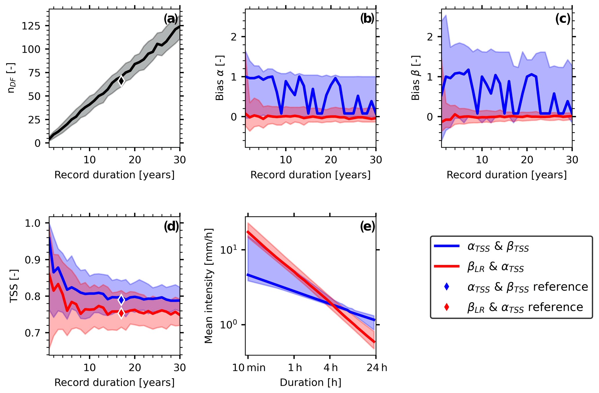
Figure 5ID-threshold sensitivity for the Illgraben catchment, assessed by resampling (bootstrapping) 100 times for each record duration (1–30 years) from the 17-year data set of debris-flow-triggering and non-triggering rainfall events. (a) Number of debris flows; (b) bias in the scale parameter α; (c) bias in the shape parameter β; (d) true skill statistic (TSS); (e) ID thresholds with variability from the observed record duration of 17 years. Solid lines are the medians, and shaded areas comprise the 10th to 90th percentiles of the resampled data. The diamonds (reference) refer to the values obtained when the full 17-year data set is used.
TSS&TSS parameter estimates are overestimated by > 100 % even after 30 years of observations, and the medians do not converge (Fig. 5b, c). The fluctuations in the median suggest that there are two to three parameter sets with TSS values which are all close to the optimum. Therefore, there are no unique ID-threshold parameters for Illgraben when estimated with TSS&TSS. The uncertainty range is not located around zero but biased towards positive values because the reference values (see Fig. 4a, solid threshold line) are at the lower end of possible solutions. The medians and the uncertainty bounds from parameters estimated with LR&TSS still converge after the reference record duration of 17 years, with biases of ±20 % for both α and β (Fig. 5b, c). However, the biases have already decreased to ±30 % after 6 years or ∼ 25 triggering events. Furthermore, the TSS score, which is overestimated for short records because it seems to be easier to fit an ID curve to only a few points, decreases and stabilizes after 6 years. Because the Illgraben record is a local data set, it is not affected by climatic, topographic, lithologic or land-use differences between sites that are present in most large-scale regional data sets. Therefore, the uncertainties can be associated with the respective method with high confidence and the Illgraben data set is well suited to studying such ID-threshold sensitivities.
Important advantages of using the TSS for ID-threshold parameter estimation are that information from both triggering and non-triggering events is considered with equal weight and that the measure is prevalence independent. However, although the narrow uncertainty range for long record durations (Fig. 5d) additionally indicates the robustness of the TSS score, it does not imply robustness in the parameter estimates that are based on the TSS (Fig. 5b, c). In our case, with 67 debris flows, the ID-threshold parameters computed with TSS&TSS seem to be highly sensitive to a few triggering events, which may be outliers but exist in any data set and are difficult to single out with certainty. Consequently, for local ID thresholds we advise against simultaneously optimizing α and β against the TSS score (TSS&TSS). Local data sets are often comparatively small (< 100 triggering events), and therefore this method can be sensitive to outliers.
Conducting the same sensitivity analysis on the regional data set showed the opposite result to that for the local data set. For the regional data set, TSS values could be slightly enhanced when using the TSS&TSS instead of the LR&TSS method (Fig. 6d), as in the local data set. In contrast to the local data set, this enhancement in the TSS is not accompanied by larger uncertainties in ID-threshold parameters (Fig. 6b, c). LR&TSS thresholds are practically flat (Fig. 6e), and parameter ranges are still converging after the reference record duration of 17 years. Using LR&TSS even makes the duration redundant because β estimated with LR&TSS converges to 0. Note that the large range in β bias for LR&TSS (Fig. 6c) is also because β is close to 0, and absolute values are small (see Sect. 3.4). TSS&TSS threshold parameters converge after ∼8 years, corresponding to ∼ 400 landslides. This is more events than reported for data sets in Italy, where ∼200 were enough both on the regional and on the national scale (Peruccacci et al., 2012, 2017).
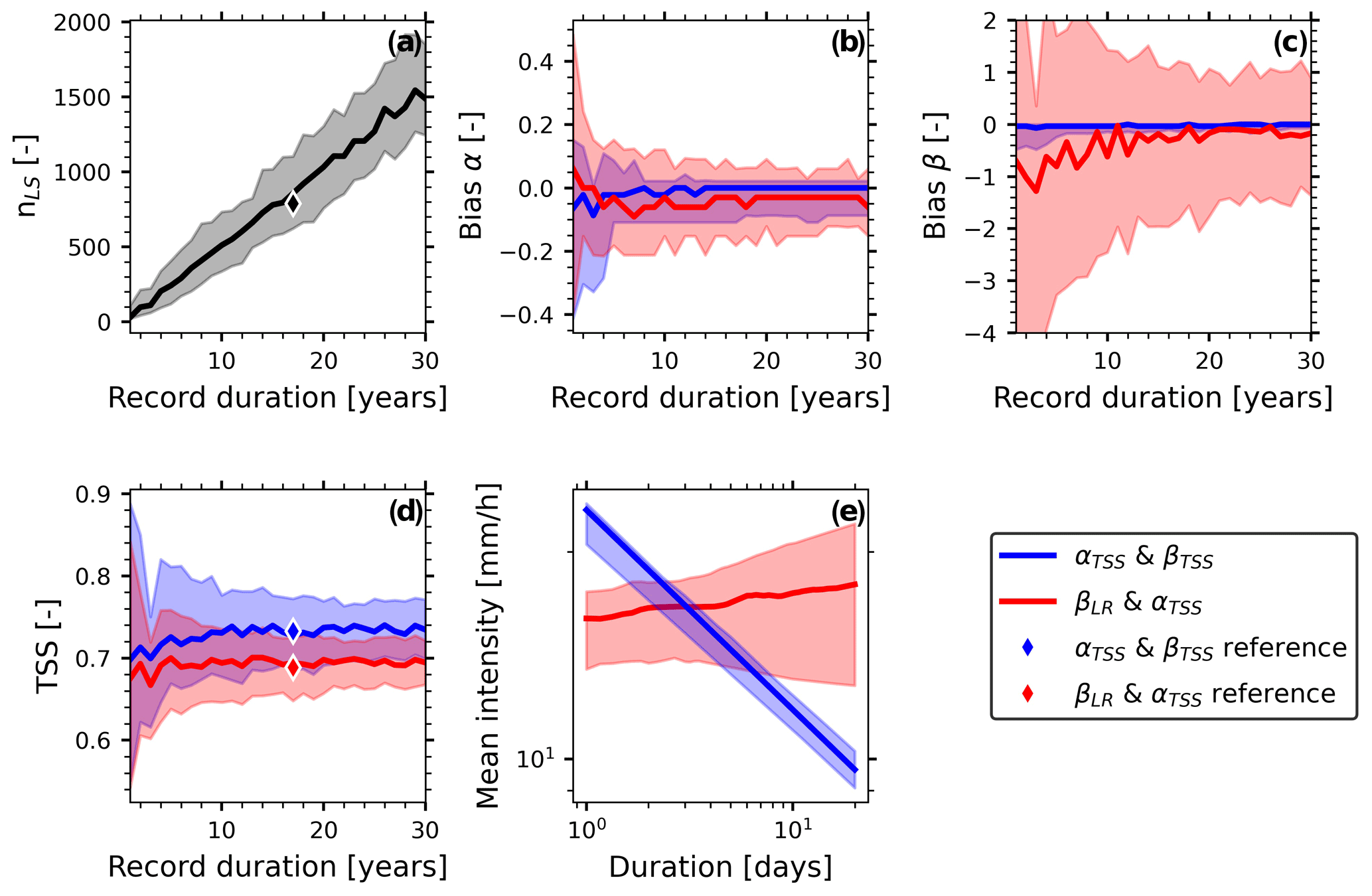
Figure 6ID-threshold sensitivity for the regional data set, assessed by resampling (bootstrapping) 100 times for each record duration (1–30 years) from the 17-year inventory of landslide-triggering and non-triggering rainfall events. (a) Number of landslides; (b) bias in the scale parameter α; (c) bias in the shape parameter β; (d) true skill statistic (TSS); (e) ID thresholds with variability from the observed record duration of 17 years. Solid lines are the medians, and shaded areas comprise the 10th to 90th percentiles of the resampled data. The diamonds (reference) refer to the values obtained when the 17-year regional data set is used.
The regional data set is inherently subject to much larger uncertainties, which can be disregarded in the local data set. These uncertainties are mainly related to climatic, topographic and lithologic differences among the landslide locations. Furthermore, the rainfall uncertainties are higher in the regional data set because the regional analyses rely on interpolated daily precipitation. As a result, the slope of the ID curve, when fitted with linear regression, may lose the typical power-law relationship of extreme rainfall. TSS&TSS instead profits more from the information in the non-triggering rainfall, by setting a threshold high enough to be above the many non-triggering rainfall events with low intensity and short duration and steep enough to detect triggering events as a response to long-lasting rainfall (Fig. 6e).
The main differences between the methods used here and the well-known frequentist method (Brunetti et al., 2010) are that non-triggering rainfall events are considered either in the determination of the scale parameter α (LR&TSS) or in both α and the shape parameter β (TSS&TSS). Parameters estimated by LR&TSS for the local data set have lower uncertainties than when estimated by TSS&TSS. For the regional data set the TSS&TSS method yields both better predictions and lower parameter uncertainty. Hence, this comparison of a local and a regional data set suggests that the range of climatic, topographic, lithologic or land-use differences within a data set should be considered when deciding which method to apply for ID-curve estimation.
4.3 Predictive power of uni- and multivariate models
We compared debris-flow-triggering proxies related to maximum rainfall intensity, antecedent rainfall and temperature, among others (Table 1, lower part). Each proxy was evaluated as a single predictor in terms of the TSS. These were also compared with five multivariate models: the LR&TSS ID threshold and four RF classifiers with different single predictors as input (Table 1, upper part). The TSS&TSS ID threshold was excluded in the further analysis due to the large uncertainties in estimated parameters. The models were validated with 5-fold cross-validation (CV).
We found that the RF classifier's TSS values (0.77–0.81) are only slightly higher than the classical ID threshold's TSS (0.76) (Fig. 7a). This improvement is due to a generally higher sensitivity score (Fig. 7b). However, as seen in the distribution of the points from the CV (with dots in Fig. 7), RF can reduce uncertainties. The best improvement in the TSS is seen when only one additional predictor (peak 30 min rainfall intensity) is added to the intensity and duration of rainfall events. If all available data are used by an RF classifier (RF_all), the performance even decreases compared with RF_ID+I-30m. This is likely due to overfitting and can happen when many of the input variables have poor predictive power. In this case, the RF classifier is fitted to the noise from the poor predictors while the predictive information from other variables is lost. Hence, CV avoids the overfitting of a model set-up, and further improvements may be achieved by testing different combinations of variables.
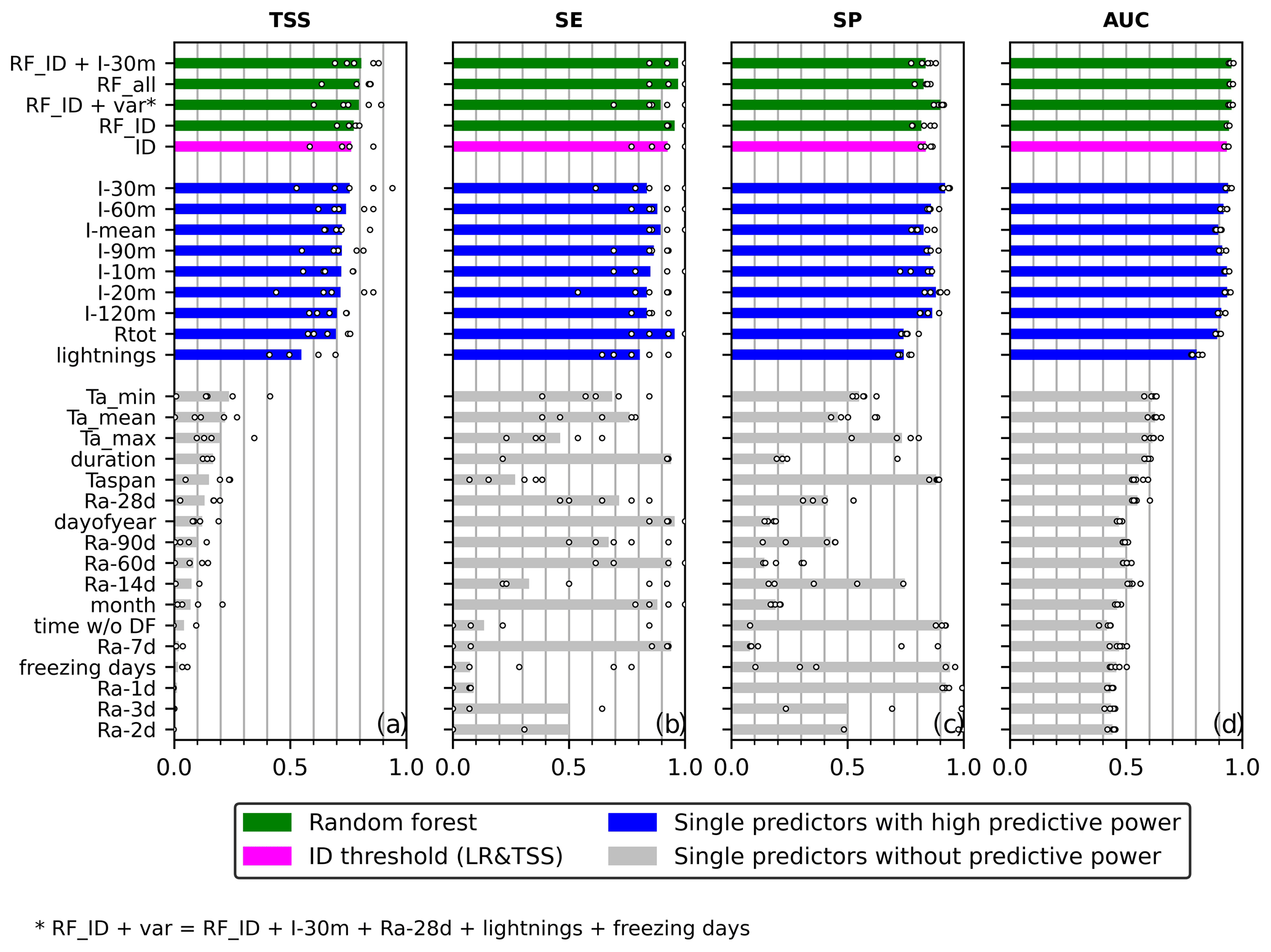
Figure 7Model comparison (see Table 1) for the prediction of debris flows in the Illgraben catchment, with reference to the (a) true skill statistic (TSS), (b) sensitivity (SE), (c) specificity (SP) and (d) area under the curve (AUC). The threshold for single predictors with predictive powers is set at AUC = 0.65. The bars refer to models using the full data set for training. The dots represent results from the 5-fold cross-validation. The models are sorted top-down with decreasing TSSs.
This analysis demonstrated that the best single predictor in terms of the TSS is the peak 30 min rainfall intensity (TSS = 0.76), and its specificity is also the highest overall (0.92) (Fig. 7c). In general, the predictors relating to maximum rainfall intensities of different timescales have relevant predictive power, while predictors related to antecedent rainfall do not. Of all debris flows, 96 % can be identified with a threshold (5 mm) for total event rainfall (Fig. 7b). Furthermore, peak 30 min rainfall intensity and mean rainfall intensity on their own perform similarly to the ID threshold. These rainfall properties are simple to calculate with a moving window from any rainfall time series, even without adding uncertainty by rainfall event separation. Surprisingly, lightning strikes also have some predictive power, even though they were recorded within an area which is almost 600 times larger than the catchment size (∼ 2800 km2). This indicates that debris flows are favourably triggered when thunderstorm clusters occur. The single predictors listed below lightning strikes in Fig. 7 have (almost) no predictive power because their AUC values are ∼ 0.5, which is close to a random guess.
Although ID thresholds are widely used in applications, a common problem is the number of false alarms they cause. For Illgraben, although 92 % of the debris flows are detected with the ID threshold estimated with LR&TSS, only 20 % of the rainfall events exceeding the threshold are expected to produce a debris flow. This performance is usually even smaller if the threshold is defined for larger spatial scales. For example, for the regional data set used here, only 0.38 % of threshold-exceeding events are expected to be landslides. This highlights the difficulties in capturing complex interactions leading to hazardous events and justifies the need to explore more data-rich approaches. Here, we systematically analysed the predictive power of single predictors and multivariate models based on the RF algorithm. Although the RF classifier only marginally improved the TSS score, the potential of overcoming some of the well-known limitations of ID thresholds is evident. For example, rainfall properties could be combined with measured, remotely sensed or modelled variables, such as discharge or soil moisture products (Wicki et al., 2020). Recently, random forests have been used to detect mass movements from seismic signals (Wenner et al., 2021; Chmiel et al., 2021) and could be coupled with rainfall measurements or forecasts to potentially increase the accuracy. It would also be interesting to study the spatio-temporal rainfall structure from radar-based rainfall estimates and its influence on debris flow triggering (Marra et al., 2016). Of course, random forests are only one alternative to ID thresholds, and there are other algorithms to be tested (see Kern et al., 2017, for a review on post-wildfire debris flows). A drawback of these empirical thresholds is that long-term observations are required to establish them. Where such data are available, additional predictors can easily be implemented in an RF classifier, as presented here, and tested regarding their predictive power.
In this study we used a 17-year record of precipitation and debris-flow timing and magnitude to complete a systematic analysis of rainfall conditions leading to debris flow triggering in a Swiss catchment, Illgraben. Based on 67 debris-flow-triggering and 1657 non-triggering rainfall events (prevalence of 3.8 %), we defined a rainfall intensity–duration threshold with the most suitable fitting method applied in this work. Given the high debris-flow frequency in Illgraben, it can be considered a lower threshold for rainfall-induced debris flows in the Swiss Rhône valley.
Debris-flow activity is greatest in summer, coinciding with peaks in total monthly rainfall accumulations and peak 30 min rainfall intensity. Although we find differences in seasonal ID thresholds, they are partly based on the occurrence of only a few triggering events (e.g. in autumn). It remains challenging to determine if the reason for this seasonality is due to seasonal differences in rainfall or in sediment availability or related to processes such as snowmelt or grain size coarsening.
Our systematic analysis of the uncertainties associated with ID thresholds shows that, for a catchment with rainfall-induced debris flows, 25 debris-flow observations are sufficient to constrain the ID-threshold parameters α and β with uncertainties of ≤ 30 %. However, our findings demonstrate that this uncertainty strongly depends on the data set and the method used to determine ID-threshold parameters. When comparing the Illgraben (local) data set with a Swiss landslide (regional) data set, more triggering events (400) were needed for threshold parameters to converge in the regional data set, due to the higher spatial variability in the data set. More importantly, the best method to minimize uncertainties changed from LR&TSS for the local to TSS&TSS for the regional data set. This underlines the need for standardized methodologies for rainfall threshold identification and validation and for proper reporting of the methods used (see Segoni et al., 2018).
Finally, we aimed to lower the false alarm rate often associated with ID thresholds. Using a random forest model including the predictors rainfall event duration, mean rainfall intensity and the peak 30 min rainfall intensity increased the TSS (true skill statistic) by 0.04 (i.e. ∼ 3 more hits or ∼ 70 fewer false alarms). Adding more input variables to the random forest model, including antecedent rainfall, did not improve the performance. Although the expectation of significantly decreasing the false alarms was not fulfilled, we present a flexible framework where additional input variables can easily be tested. The aim of future work should be to include variables such as modelled or measured soil moisture or information on spatio-temporal rainfall structure from radar-based rainfall estimates. Machine learning algorithms can be helpful for maximizing information exploitation from available data and for increasing the accuracy of (debris-flow) early warning systems, and we have highlighted this potential.
The source code with an example data set is available from the Environmental Data Portal (EnviDat) (https://doi.org/10.16904/envidat.240; Hirschberg, 2021). The debris-flow volumes are also available from EnviDat (https://doi.org/10.16904/envidat.173; McArdell and Hirschberg, 2020). Climate data are available for research purposes from the agencies mentioned in Sect. 3.1.
JH conducted the analysis, produced the figures and wrote the original article draft. JH, AB, BWM and PM designed the study. EL provided the metadata of the regional data set and guided the analysis. All authors contributed to the interpretation of the results and to the revision of the article.
The contact author has declared that neither they nor their co-authors have any competing interests.
Publisher’s note: Copernicus Publications remains neutral with regard to jurisdictional claims in published maps and institutional affiliations.
We thank MeteoSwiss for providing climate data and the municipality of Leuk for providing rainfall data. We thank Melissa Dawes for improving the use of English in an earlier version of this paper. Finally, we thank Ben Mirus and Clàudia Abancó for their constructive reviews, which helped to improve the manuscript.
This research has been supported by the WSL research programme CCAMM (Climate Change Impacts on Alpine Mass Movements) and by the Swiss National Science Foundation (grant no. 165979).
This paper was edited by Thomas Glade and reviewed by Clàudia Abancó and Ben Mirus.
Abancó, C., Hürlimann, M., Moya, J., and Berenguer, M.: Critical rainfall conditions for the initiation of torrential flows. Results from the Rebaixader catchment (Central Pyrenees), J. Hydrol., 541, 218–229, https://doi.org/10.1016/j.jhydrol.2016.01.019, 2016. a, b, c
Badoux, A., Graf, C., Rhyner, J., Kuntner, R., and McArdell, B. W.: A debris-flow alarm system for the Alpine Illgraben catchment: Design and performance, Nat. Hazards, 49, 517–539, https://doi.org/10.1007/s11069-008-9303-x, 2009. a, b, c, d
Badoux, A., Turowski, J. M., Mao, L., Mathys, N., and Rickenmann, D.: Rainfall intensity–duration thresholds for bedload transport initiation in small Alpine watersheds, Nat. Hazards Earth Syst. Sci., 12, 3091–3108, https://doi.org/10.5194/nhess-12-3091-2012, 2012. a, b
Badoux, A., Andres, N., Techel, F., and Hegg, C.: Natural hazard fatalities in Switzerland from 1946 to 2015, Nat. Hazards Earth Syst. Sci., 16, 2747–2768, https://doi.org/10.5194/nhess-16-2747-2016, 2016. a
Bel, C., Liébault, F., Navratil, O., Eckert, N., Bellot, H., Fontaine, F., and Laigle, D.: Rainfall control of debris- flow triggering in the Réal Torrent, Southern French Prealps, Geomorphology, 291, 17–32, https://doi.org/10.1016/j.geomorph.2016.04.004, 2017. a, b, c, d, e, f, g, h, i, j
Bennett, G. L., Molnar, P., Eisenbeiss, H., and Mcardell, B. W.: Erosional power in the Swiss Alps: Characterization of slope failure in the Illgraben, Earth Surf. Proc. Land., 37, 1627–1640, https://doi.org/10.1002/esp.3263, 2012. a
Bennett, G. L., Molnar, P., McArdell, B. W., and Burlando, P.: A probabilistic sediment cascade model of sediment transfer in the Illgraben, Water Resour. Res., 50, 1225–1244, https://doi.org/10.1002/2013WR013806, 2014. a
Berger, C., McArdell, B. W., and Schlunegger, F.: Sediment transfer patterns at the Illgraben catchment, Switzerland: Implications for the time scales of debris flow activities, Geomorphology, 125, 421–432, https://doi.org/10.1016/j.geomorph.2010.10.019, 2011. a, b
Berti, M. and Simoni, A.: Experimental evidences and numerical modelling of debris flow initiated by channel runoff, Landslides, 2, 171–182, https://doi.org/10.1007/s10346-005-0062-4, 2005. a
Berti, M., Bernard, M., Simoni, A., and Gregoretti, C.: Physical interpretation of rainfall thresholds for runoff-generated debris flows, J. Geophys. Res.-Earth, 125, 1–25, https://doi.org/10.1029/2019JF005513, 2020. a
Bogaard, T. and Greco, R.: Invited perspectives: Hydrological perspectives on precipitation intensity-duration thresholds for landslide initiation: proposing hydro-meteorological thresholds, Nat. Hazards Earth Syst. Sci., 18, 31–39, https://doi.org/10.5194/nhess-18-31-2018, 2018. a
Breiman, L.: Random forests, Mach. Learn., 45, 5–32, https://doi.org/10.1023/A:1010933404324, 2001. a, b, c
Brunetti, M. T., Peruccacci, S., Rossi, M., Luciani, S., Valigi, D., and Guzzetti, F.: Rainfall thresholds for the possible occurrence of landslides in Italy, Nat. Hazards Earth Syst. Sci., 10, 447–458, https://doi.org/10.5194/nhess-10-447-2010, 2010. a, b
Caine, N.: The Rainfall Intensity -Duration Control of Shallow Landslides and Debris Flows, Geogr. Ann. A, 62, 23–27, https://doi.org/10.1080/04353676.1980.11879996, 1980. a, b, c
Cannon, S. H., Gartner, J. E., Rupert, M. G., Michael, J. A., Rea, A. H., and Parrett, C.: Predicting the probability and volume of postwildfire debris flows in the intermountain western United States, Bull. Geol. Soc. Am., 122, 127–144, https://doi.org/10.1130/B26459.1, 2010. a, b
Chmiel, M., Walter, F., Wenner, M., Zhang, Z., McArdell, B. W., and Hibert, C.: Machine Learning Improves Debris Flow Warning, Geophys. Res. Lett., 48, e2020GL090874, https://doi.org/10.1029/2020GL090874, 2021. a
Coe, J. A., Kinner, D. A., and Godt, J. W.: Initiation conditions for debris flows generated by runoff at Chalk Cliffs, central Colorado, Geomorphology, 96, 270–297, https://doi.org/10.1016/j.geomorph.2007.03.017, 2008. a, b, c
de Haas, T., Nijland, W., de Jong, S. M., and Mcardell, B. W.: How memory effects, check dams, and channel geometry control erosion and deposition by debris flows, Sci. Rep.-UK, 10, 1–8, https://doi.org/10.1038/s41598-020-71016-8, 2020. a
Deganutti, A. M., Marchi, L., and Arattano, M.: Raindall and debris-flow occurrence in the Moscardo basin (Italian Alps), in: Debris-Flow Mitigation: Mechanics, Prediction, and Assessment, edited by: Wieczorek, G. and Naeser, N., Balkema, Rotterdam, Netherlands, 67–72, 2000. a, b
Domènech, G., Fan, X., Scaringi, G., van Asch, T. W., Xu, Q., Huang, R., and Hales, T. C.: Modelling the role of material depletion, grain coarsening and revegetation in debris flow occurrences after the 2008 Wenchuan earthquake, Eng. Geol., 250, 34–44, https://doi.org/10.1016/j.enggeo.2019.01.010, 2019. a
Dowling, C. A. and Santi, P. M.: Debris flows and their toll on human life: A global analysis of debris-flow fatalities from 1950 to 2011, Nat. Hazards, 71, 203–227, https://doi.org/10.1007/s11069-013-0907-4, 2014. a
Dunkerley, D.: Identifying individual rain events from pluviograph records: A review with analysis of data from an Australian dryland site, Hydrol. Process., 22, 5024–5036, https://doi.org/10.1002/hyp.7122, 2008. a
Fawcett, T.: An introduction to ROC analysis, Pattern Recogn. Lett., 27, 861–874, https://doi.org/10.1016/j.patrec.2005.10.010, 2006. a
Frei, C. and Schär, C.: A precipitation climatology of the Alps from high-resolution rain-gauge observations, Int. J. Climatol., 18, 873–900, https://doi.org/10.1002/(SICI)1097-0088(19980630)18:8<873::AID-JOC255>3.0.CO;2-9, 1998. a
Fryxwell, F. M. and Horberg, L.: Alpine mudflows in Grand Teton National Park, Wyoming, GSA Bulletin, 54, 457–472, https://doi.org/10.1130/GSAB-54-457, 1943. a
Gaál, L., Molnar, P., and Szolgay, J.: Selection of intense rainfall events based on intensity thresholds and lightning data in Switzerland, Hydrol. Earth Syst. Sci., 18, 1561–1573, https://doi.org/10.5194/hess-18-1561-2014, 2014. a, b, c
Gariano, S. L., Brunetti, M. T., Iovine, G., Melillo, M., Peruccacci, S., Terranova, O., Vennari, C., and Guzzetti, F.: Calibration and validation of rainfall thresholds for shallow landslide forecasting in Sicily, southern Italy, Geomorphology, 228, 653–665, https://doi.org/10.1016/j.geomorph.2014.10.019, 2015. a
Gariano, S. L., Melillo, M., Peruccacci, S., and Brunetti, M. T.: How much does the rainfall temporal resolution affect rainfall thresholds for landslide triggering?, Nat. Hazards, 100, 655–670, https://doi.org/10.1007/s11069-019-03830-x, 2020. a
Gregoretti, C.: The initiation of debris flow at high slopes: Experimental results, J. Hydraul. Res., 38, 83–88, https://doi.org/10.1080/00221680009498343, 2000. a
Guzzetti, F., Peruccacci, S., Rossi, M., and Stark, C. P.: Rainfall thresholds for the initiation of landslides in central and southern Europe, Meteorol. Atmos. Phys., 98, 239–267, https://doi.org/10.1007/s00703-007-0262-7, 2007. a
Guzzetti, F., Gariano, S. L., Peruccacci, S., Brunetti, M. T., Marchesini, I., Rossi, M., and Melillo, M.: Geographical landslide early warning systems, Earth-Sci. Rev., 200, 102973, https://doi.org/10.1016/j.earscirev.2019.102973, 2020. a
Hanssen, A. W. and Kuipers, W. J. A.: On the relationship between the frequency of rain and various meteorological parameters, Meded. Verh, 81, 2–15, 1965. a
Hilker, N., Badoux, A., and Hegg, C.: The Swiss flood and landslide damage database 1972–2007, Nat. Hazards Earth Syst. Sci., 9, 913–925, https://doi.org/10.5194/nhess-9-913-2009, 2009. a, b
Hirschberg, J.: Source code for: Evaluating methods for debris-flow prediction based on rainfall in an Alpine catchment, EnviDat [code], https://doi.org/10.16904/envidat.240, 2021. a
Hirschberg, J., McArdell, B. W., Badoux, A., and Molnar, P.: Analysis of rainfall and runoff for debris flows at the Illgraben catchment, Switzerland, in: Debris-Flow Hazards Mitigation: Mechanics, Monitoring, Modeling, and Assessment – Proceedings of the 7th International Conference on Debris-Flow Hazards Mitigation, 693–700, 2019. a, b
Hirschberg, J., Fatichi, S., Bennett, G. L., McArdell, B. W., Peleg, N., Lane, S. N., Schlunegger, F., and Molnar, P.: Climate Change Impacts on Sediment Yield and Debris-Flow Activity in an Alpine Catchment, J. Geophys. Res.-Earth, 126, e2020JF005739, https://doi.org/10.1029/2020JF005739, 2021. a, b, c, d
Hungr, O., Leroueil, S., and Picarelli, L.: The Varnes classification of landslide types, an update, Landslides, 11, 167–194, https://doi.org/10.1007/s10346-013-0436-y, 2014. a
Hürlimann, M., Rickenmann, D., and Graf, C.: Field and monitoring data of debris-flow events in the Swiss Alps, Can. Geotech. J., 40, 161–175, https://doi.org/10.1139/t02-087, 2003. a, b, c
Hydrological Atlas of Switzerland: Mean Precipitation, [data set], available at: https://hydrologicalatlas.ch (last access: 4 September 2020-09-), 2015. a
Iverson, R. M.: The Physics of Debris Flows, Rev. Geophys., 35, 245–296, https://doi.org/10.1029/97RG00426, 1997. a
Iverson, R. M., Reid, M. E., Logan, M., LaHusen, R. G., Godt, J. W., and Griswold, J. P.: Positive feedback and momentum growth during debris-flow entrainment of wet bed sediment, Nat. Geosci., 4, 116–121, https://doi.org/10.1038/ngeo1040, 2011. a
James, G., Witten, D., Hastie, T., and Tibshirani, R.: Resampling Methods, Springer New York, New York, NY, 175–201, https://doi.org/10.1007/978-1-4614-7138-7_5, 2013a. a
James, G., Witten, D., Hastie, T., and Tibshirani, R.: Tree-Based Methods, Springer New York, New York, NY, 303–335, https://doi.org/10.1007/978-1-4614-7138-7_8, 2013b. a
Johnson, A. M. and Rodine, J. D.: Debris flow, in: Slope instability, edited by: Brunsden, D. and Prior, D., Wiley and Sons, Chichester, England, 1984. a
Kern, A. N., Addison, P., Oommen, T., Salazar, S. E., and Coffman, R. A.: Machine Learning Based Predictive Modeling of Debris Flow Probability Following Wildfire in the Intermountain Western United States, Math. Geosci., 49, 717–735, https://doi.org/10.1007/s11004-017-9681-2, 2017. a, b
Leonarduzzi, E. and Molnar, P.: Deriving rainfall thresholds for landsliding at the regional scale: daily and hourly resolutions, normalisation, and antecedent rainfall, Nat. Hazards Earth Syst. Sci., 20, 2905–2919, https://doi.org/10.5194/nhess-20-2905-2020, 2020. a, b, c, d, e, f
Leonarduzzi, E., Molnar, P., and McArdell, B. W.: Predictive performance of rainfall thresholds for shallow landslides in Switzerland from gridded daily data, Water Resour. Res., 53, 6612–6625, https://doi.org/10.1002/2017WR021044, 2017. a, b, c, d, e
Lichtenhahn, C.: Zwei Betonmauern: die Geschieberückhaltesperre am Illgraben [Wallis] und die Staumauer des Hochwasserschutzbeckens an der Orlegna im Bergell [Graubünden], Internationales Symposium Interpraevent, Villach, Austria: F.f.v. Hochwasserbekämpfung, 451–456, 1971. a
Marra, F.: Rainfall thresholds for landslide occurrence: systematic underestimation using coarse temporal resolution data, Nat. Hazards, 95, 889–890, https://doi.org/10.1007/s11069-018-3508-4, 2019. a
Marra, F., Nikolopoulos, E. I., Creutin, J. D., and Borga, M.: Space–time organization of debris flows-triggering rainfall and its effect on the identification of the rainfall threshold relationship, J. Hydrol., 541, 246–255, https://doi.org/10.1016/j.jhydrol.2015.10.010, 2016. a, b, c
McArdell, B. W.: Field Measurements of Forces in Debris Flows at the Illgraben: Implications for Channel-Bed Erosion, International Journal of Erosion Control Engineering, 9, 194–198, https://doi.org/10.13101/ijece.9.194, 2016. a
McArdell, B. W. and Badoux, A.: Influence of rainfall on the initiation of debris flows at the Illgraben catchment, canton of Valais, Switzerland, in: Geophysical Research Abstracts, 9, 8804, 2007. a
McArdell, B. W. and Hirschberg, J.: Debris-flow volumes at the Illgraben 2000–2017, EnviDat [data set], https://doi.org/10.16904/envidat.173, 2020. a, b, c
McArdell, B. W. and Sartori, M.: The Illgraben Torrent System, 367–378, Springer International Publishing, Cham, https://doi.org/10.1007/978-3-030-43203-4_25, 2021. a
McArdell, B. W., Bartelt, P., and Kowalski, J.: Field observations of basal forces and fluid pore pressure in a debris flow, Geophys. Res. Lett., 34, 2–5, https://doi.org/10.1029/2006GL029183, 2007. a
McCoy, S. W., Kean, J. W., Coe, J. A., Tucker, G. E., Staley, D. M., and Wasklewicz, T. A.: Sediment entrainment by debris flows: In situ measurements from the headwaters of a steep catchment, J. Geophys. Res.-Earth, 117, F03016, https://doi.org/10.1029/2011JF002278, 2012. a
Mirus, B., Morphew, M., and Smith, J.: Developing Hydro-Meteorological Thresholds for Shallow Landslide Initiation and Early Warning, Water, 10, 1274, https://doi.org/10.3390/w10091274, 2018. a, b
Mostbauer, K., Kaitna, R., Prenner, D., and Hrachowitz, M.: The temporally varying roles of rainfall, snowmelt and soil moisture for debris flow initiation in a snow-dominated system, Hydrol. Earth Syst. Sci., 22, 3493–3513, https://doi.org/10.5194/hess-22-3493-2018, 2018. a
Nikolopoulos, E. I., Destro, E., Bhuiyan, M. A. E., Borga, M., and Anagnostou, E. N.: Evaluation of predictive models for post-fire debris flow occurrence in the western United States, Nat. Hazards Earth Syst. Sci., 18, 2331–2343, https://doi.org/10.5194/nhess-18-2331-2018, 2018. a, b, c, d
Nikolopoulos, E. I., Crema, S., Marchi, L., Marra, F., Guzzetti, F., and Borga, M.: Impact of uncertainty in rainfall estimation on the identification of rainfall thresholds for debris flow occurrence, Geomorphology, 221, 286–297, https://doi.org/10.1016/j.geomorph.2014.06.015, 2014. a, b
Papa, M. N., Medina, V., Ciervo, F., and Bateman, A.: Derivation of critical rainfall thresholds for shallow landslides as a tool for debris flow early warning systems, Hydrol. Earth Syst. Sci., 17, 4095–4107, https://doi.org/10.5194/hess-17-4095-2013, 2013. a
Pastorello, R., Hürlimann, M., and D'Agostino, V.: Correlation between the rainfall, sediment recharge, and triggering of torrential flows in the Rebaixader catchment (Pyrenees, Spain), Landslides, 15, 1921–1934, https://doi.org/10.1007/s10346-018-1000-6, 2018. a
Pedregosa, F., Michel, V., Varoquaux, G., Thirion, B., Dubourg, V., Passos, A., Perrot, M., Grisel, O., Blondel, M., Prettenhofer, P., Weiss, R., Vanderplas, J., Cournapeau, D., Pedregosa, F., Varoquaux, G., Gramfort, A., Thirion, B., Grisel, O., Dubourg, V., Passos, A., Brucher, M., Perrot andÉdouardand, M., and Duchesnay, É.: Scikit-learn: Machine Learning in Python, J. Machine Learn. Res., 12, 2825–2830, 2011. a
Peirce, C. S.: The numerical measure of the success of predictions, Science, 4, 453–454, https://doi.org/10.1126/science.ns-4.93.453-a, 1884. a
Peruccacci, S., Brunetti, M. T., Luciani, S., Vennari, C., and Guzzetti, F.: Lithological and seasonal control on rainfall thresholds for the possible initiation of landslides in central Italy, Geomorphology, 139–140, 79–90, https://doi.org/10.1016/j.geomorph.2011.10.005, 2012. a
Peruccacci, S., Brunetti, M. T., Gariano, S. L., Melillo, M., Rossi, M., and Guzzetti, F.: Rainfall thresholds for possible landslide occurrence in Italy, Geomorphology, 290, 39–57, https://doi.org/10.1016/j.geomorph.2017.03.031, 2017. a
Postance, B., Hillier, J., Dijkstra, T., and Dixon, N.: Comparing threshold definition techniques for rainfall-induced landslides: A national assessment using radar rainfall, Earth Surf. Proc. Land., 43, 553–560, https://doi.org/10.1002/esp.4202, 2018. a
Reichstein, M., Camps-Valls, G., Stevens, B., Jung, M., Denzler, J., Carvalhais, N., and Prabhat: Deep learning and process understanding for data-driven Earth system science, Nature, 566, 195–204, https://doi.org/10.1038/s41586-019-0912-1, 2019. a
Rickenmann, D., Hürlimann, M., Graf, C., Näf, D., and Weber, D.: Murgang-Beobachtungsstationen in der Schweiz, in: Wasser Energie Luft, 93, 1–8, 2001. a
Schlunegger, F., Badoux, A., McArdell, B. W., Gwerder, C., Schnydrig, D., Rieke-Zapp, D., and Molnar, P.: Limits of sediment transfer in an alpine debris-flow catchment, Illgraben, Switzerland, Quaternary Sci. Rev., 28, 1097–1105, https://doi.org/10.1016/j.quascirev.2008.10.025, 2009. a, b
Schneuwly-Bollschweiler, M. and Stoffel, M.: Hydrometeorological triggers of periglacial debris flows in the Zermatt valley (Switzerland) since 1864, J. Geophys. Res.-Earth, 117, 1–12, https://doi.org/10.1029/2011JF002262, 2012. a
Segoni, S., Piciullo, L., and Gariano, S. L.: A review of the recent literature on rainfall thresholds for landslide occurrence, Landslides, 15, 1483–1501, https://doi.org/10.1007/s10346-018-0966-4, 2018. a, b, c
Stähli, M., Sättele, M., Huggel, C., McArdell, B. W., Lehmann, P., Van Herwijnen, A., Berne, A., Schleiss, M., Ferrari, A., Kos, A., Or, D., and Springman, S. M.: Monitoring and prediction in early warning systems for rapid mass movements, Nat. Hazards Earth Syst. Sci., 15, 905–917, https://doi.org/10.5194/nhess-15-905-2015, 2015. a
Staley, D. M., Kean, J. W., Cannon, S. H., Schmidt, K. M., and Laber, J. L.: Objective definition of rainfall intensity-duration thresholds for the initiation of post-fire debris flows in southern California, Landslides, 10, 547–562, https://doi.org/10.1007/s10346-012-0341-9, 2013. a, b, c, d
Staley, D. M., Negri, J. A., Kean, J. W., Laber, J. L., Tillery, A. C., and Youberg, A. M.: Prediction of spatially explicit rainfall intensity–duration thresholds for post-fire debris-flow generation in the western United States, Geomorphology, 278, 149–162, https://doi.org/10.1016/j.geomorph.2016.10.019, 2017. a, b
Takahashi, T.: Mechanical Characteristics of Debris Flow, J. Hydr. Eng. Div.-ASCE, 104, 1153–1169, 1978. a
Takahashi, T.: Debris Flow, Annu. Rev. Fluid Mech., 13, 57–77, https://doi.org/10.1146/annurev.fl.13.010181.000421, 1981. a
Tang, H., McGuire, L. A., Rengers, F. K., Kean, J. W., Staley, D. M., and Smith, J. B.: Developing and Testing Physically Based Triggering Thresholds for Runoff-Generated Debris Flows, Geophys. Res. Lett., 46, 8830–8839, https://doi.org/10.1029/2019GL083623, 2019. a
Tognacca, C.: Beitrag zur Untersuchung der Entstehungsmechanismen von Murgangen, Phd thesis, ETH Zürich, Zürich, https://doi.org/10.3929/ethz-a-010025751, 1999. a
Wenner, M., Hibert, C., van Herwijnen, A., Meier, L., and Walter, F.: Near-real-time automated classification of seismic signals of slope failures with continuous random forests, Nat. Hazards Earth Syst. Sci., 21, 339–361, https://doi.org/10.5194/nhess-21-339-2021, 2021. a
Wicki, A., Lehmann, P., Hauck, C., Seneviratne, S. I., Waldner, P., and Stähli, M.: Assessing the potential of soil moisture measurements for regional landslide early warning, Landslides, 17, 1881–1896, https://doi.org/10.1007/s10346-020-01400-y, 2020. a
Youden, W. J.: Index for rating diagnostic tests, Cancer, 3, 32–35, https://doi.org/10.1002/1097-0142(1950)3:1<32::AID-CNCR2820030106>3.0.CO;2-3, 1950. a