the Creative Commons Attribution 4.0 License.
the Creative Commons Attribution 4.0 License.
 | 08 Sep 2021
Timely prediction potential of landslide early warning systems with multispectral remote sensing: a conceptual approach tested in the Sattelkar, Austria
Markus Keuschnig
Ingo Hartmeyer
Robert Delleske
Michael Krautblatter
While optical remote sensing has demonstrated its capabilities for landslide detection and monitoring, spatial and temporal demands for landslide early warning systems (LEWSs) had not been met until recently. We introduce a novel conceptual approach to structure and quantitatively assess lead time for LEWSs. We analysed “time to warning” as a sequence: (i) time to collect, (ii) time to process and (iii) time to evaluate relevant optical data. The difference between the time to warning and “forecasting window” (i.e. time from hazard becoming predictable until event) is the lead time for reactive measures. We tested digital image correlation (DIC) of best-suited spatiotemporal techniques, i.e. 3 m resolution PlanetScope daily imagery and 0.16 m resolution unmanned aerial system (UAS)-derived orthophotos to reveal fast ground displacement and acceleration of a deep-seated, complex alpine mass movement leading to massive debris flow events. The time to warning for the UAS/PlanetScope totals 31/21 h and is comprised of time to (i) collect – 12/14 h, (ii) process – 17/5 h and (iii) evaluate – 2/2 h, which is well below the forecasting window for recent benchmarks and facilitates a lead time for reactive measures. We show optical remote sensing data can support LEWSs with a sufficiently fast processing time, demonstrating the feasibility of optical sensors for LEWSs.
- Article
(11931 KB) - Full-text XML
-
Supplement
(10743 KB) - BibTeX
- EndNote


Landslides are a major natural hazard leading to human casualties and socio-economic impacts, mainly by causing infrastructure damage (Dikau et al., 1996; Hilker et al., 2009). They are often triggered by earthquakes, intense short-period or prolonged precipitation, and human activities (Hungr et al., 2014; Froude and Petley, 2018). In a systematic review Gariano and Guzzetti (2016) report that 80 % of the papers examined show causal relationships between landslides and climate change. The ongoing warming of the climate (IPCC, 2014) is likely to decrease slope stability and increase landslide activity (Huggel et al., 2012; Seneviratne et al., 2012), which indicates a vital need to improve the ability to detect, monitor and issue early warnings of landslides and thus to reduce and mitigate landslide risk.
Early warning refers to a set of capacities for the timely and effective provision of warning information through institutions, such that individuals, communities and organisations exposed to a hazard are able to take action with sufficient time to reduce or avoid risk and prepare an effective response (UNISDR, 2009). According to UNISDR (2006), an effective early warning system consists of four elements: (1) risk knowledge, the systematic data collection and risk assessment; (2) the monitoring and warning service; (3) the dissemination and communication of risk as well as early warnings; and (4) the response capabilities on local and national levels. Lead time as defined in the context of landslide early warning systems (LEWSs) is the interval between the issue of a warning (i.e. dissemination) and the forecasted landslide onset (Pecoraro et al., 2019) and thus crucially depends on time requirements in phases (1)–(3). The success of an early warning system (EWS) therefore requires measurable pre-failure motion (or slow slope displacement) to allow for sufficient lead time for decisions on reactions and countermeasures (Grasso, 2014; Hungr et al., 2014).
While remote sensing has been established for early warnings, remote sensing is not yet used for real early warnings of the onset of landslides in steep alpine terrain (with a few exceptions), where geotechnical instruments are still preferred. Exceptions include terrestrial InSAR (Pesci et al., 2011; Walter et al., 2020) and terrestrial laser scanning with high repetition rates. However, repeated UAS (unmanned aerial system) and optical satellite (PlanetScope) images with high repetition rates have so far not been applied for landslide early warning in steep alpine catchments. In this regard, knowledge of sensor capabilities and limitations is essential, as it determines which rates and magnitudes of pre-failure motion can potentially be identified (Desrues et al., 2019). Our proposed framework refers to mass movements in steep alpine catchments with significant pre-failure motion over sufficient time periods and thus excludes instantaneous events triggered by processes such as heavy rainfalls or earthquakes.
This study presents a new concept to systematically evaluate remote sensing techniques to estimate and increase lead time for landslide early warnings in these catchments. We do not start from the perspective of available data; instead, we define necessary time constraints to successfully employ remote sensing data to provide early warnings. This approach reduces to a small number the suitable remote sensing products with high temporal and spatial resolutions. With these constraints, we investigated the application of data from satellites and UASs to allow the assessment of the data, after a spaceborne area-wide but low-resolution acquisition, into a downscaled detailed image recording. In so doing, we analysed the capability of these different passive remote sensing systems focusing on spatiotemporal capabilities for ground motion detection and landslide evolution to provide early warnings.
Recently, the spatial and temporal resolution of optical satellite imagery has significantly improved (Scaioni et al., 2014) and has allowed substantial advances in the definition of displacement rates and acceleration thresholds to approach requirements for early warning purposes. This is essential since the spatial and temporal resolution determine whether landslide monitoring is possible with the detection of displacement rates and approximate acceleration thresholds, both of which are lacking if information is based solely on post-event studies (Reid et al., 2008; Calvello, 2017). Landslide monitoring offers the potential to significantly advance LEWSs (Chae et al., 2017; Crosta et al., 2017). Previously, high-spatial-resolution satellite data were obtained at the expense of a reduction in the revisit rates (Aubrecht et al., 2017). Consequently, the return period between two images increased, limiting ground displacement assessment and the range of observable motion rates. The number of useful images was further reduced due to natural factors such as snow cover, cloud cover and cloud shadows. High-resolution remote sensing data were long restricted due to high costs and data volume (Goodchild, 2011; Westoby et al., 2012). Today commercial very high resolution (VHR) optical satellites exist, but tasked acquisitions make them inflexible and very cost intensive, thus limiting research (Butler, 2014; Lucieer et al., 2014). There is a vast spectrum of available remote sensing data with a high spatiotemporal resolution (Table 1). Complementary use of different remote sensing sources can significantly improve landslide assessment as demonstrated by Stumpf et al. (2018) and Bontemps et al. (2018), who draw on archive data and utilise different sensor combinations to analyse the evolution of ground motion.
Table 1Overview of different optical multispectral remote sensors with their corresponding resolution [m] and revisit rate [d]. The sensors are categorised into commercial and free data policy. Source: ESA (2020).
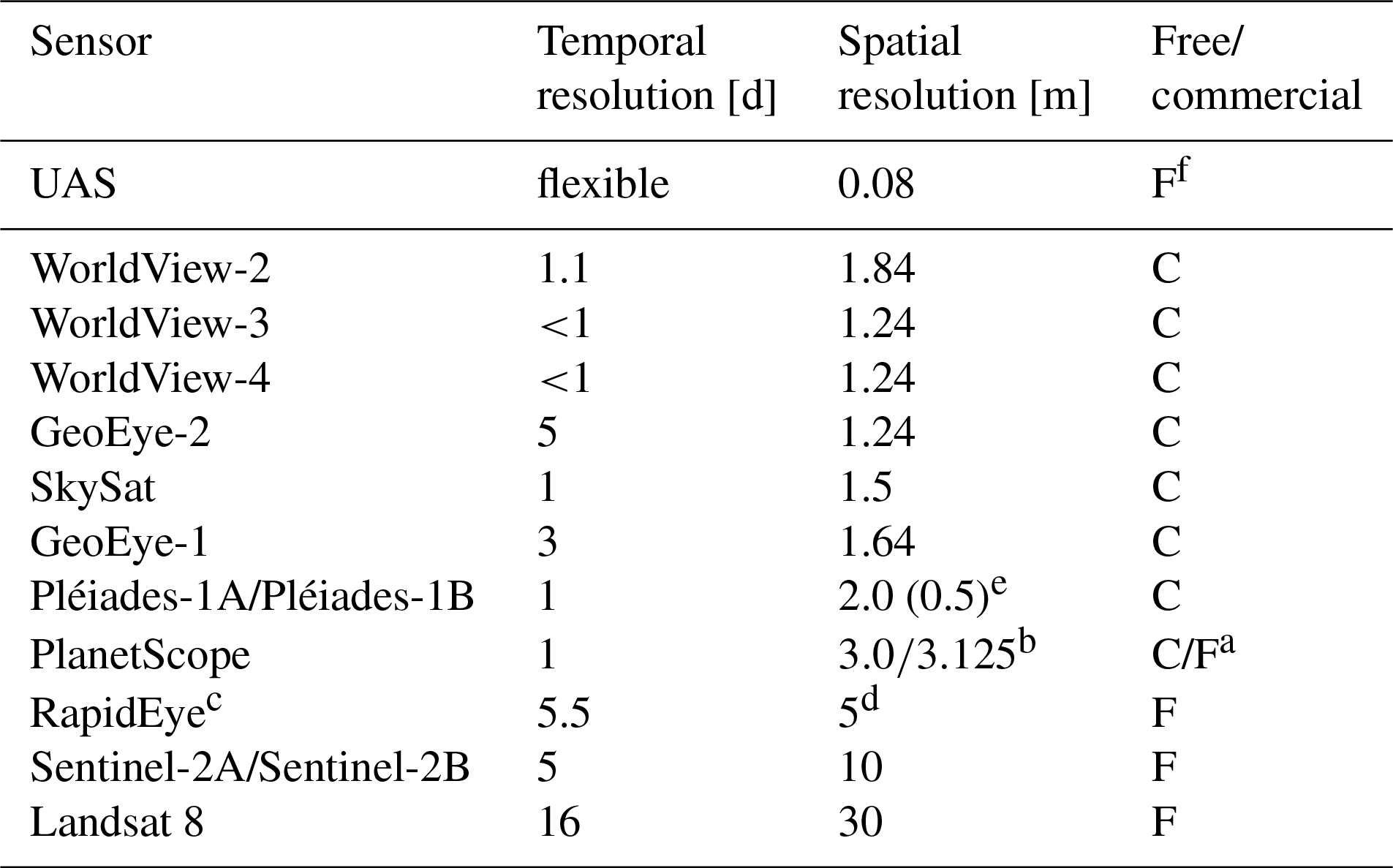
a Free quota via Planet's Education and Research Program. b PlanetScope Ortho Scene product, Level 3B/Ortho Tile product, Level 3A (Planet Labs, 2020b). c Reached end of life, March 2020, archive data usable. d Ortho Tile Level 3A, 5 m (Planet Labs, 2020a). e Colour pansharpened, 0.5 m. f Self-acquired.
The latest developments in Earth observation programmes include both the new Copernicus Sentinel fleet operated by ESA and a new generation of micro cube satellites, sent into orbit in large numbers by Planet Labs, Inc. These micro cube satellites, known as “Doves” as part of PlanetScope (from now on referred to as PlanetScope satellites), and Sentinel-2A and Sentinel-2B offer very high revisit rates of 1–5 d and high spatial resolutions of 3 and 10 m, respectively (Table 1), for multispectral imagery (Drusch et al., 2012; Butler, 2014; Breger, 2017). These high spatiotemporal resolutions open up unprecedented possibilities of studying a wide range of landslide velocities and natural hazards through remote sensing. Continuing data access is fostered by Planet Labs and by Copernicus (via its open data policy) providing affordable or free data for research. Examples of landslide activity studies employing multi-temporal datasets based on this access to high-spatiotemporal-resolution data include Lacroix et al. (2018), using Sentinel-2 scenes to detect motions of the Harmalière landslide in France, and Mazzanti et al. (2020), who applied a large stack of PlanetScope images for the active Rattlesnake landslide, USA.
As landslides tend to accelerate beyond the deformation rate observable with radar systems before failure, we concentrate on optical image analysis (Moretto et al., 2016). One advantage of optical imagery is its temporally dense data (Table 1) compared to open data radar systems with a sensor repeat frequency of 6 d and revisit frequency of 3 d at the Equator, about 2 d over Europe and less than 1 d at high latitudes (Sentinel-1, ESA). Optical data allow direct visual impressions from the multispectral representation of the acquisition target and the option to employ these data for further complementary and expert analyses. While active radar systems overcome constraints posed by clouds and do not require daylight, data voids can be significant due to layover or shadowing effects in steep mountainous areas (Mazzanti et al., 2012; Plank et al., 2015; Moretto et al., 2016). Moreover, north-/south-facing slopes are less suitable and thus limit the range of investigation (Darvishi et al., 2018). In general, sensor choice depends on the landslide motion rate with radar at the lower and optical instruments at the upper motion range (Crosetto et al., 2016; Moretto et al., 2017; Lacroix et al., 2019).
However, a flexible, cost-effective alternative to spaceborne optical data is airborne optical images taken by UASs. Freely selectable flight routes and acquisition dates enable avoiding shadows from clouds and topographic obstacles as well as unfavourable weather conditions and summertime snow cover, all of which frequently impair satellite images (Giordan et al., 2018; Lucieer et al., 2014). UAS-based surveys provide accurate very high resolution (a few centimetres) orthoimages and digital elevation models (DEMs) of relatively small areas, suitable for detailed, repeated analyses and geomorphological applications (Westoby et al., 2012; Turner et al., 2015).
In recent years, data provision for users has increased, and today data hubs provide easy accessibility to rapid, pre-processed imagery. Nonetheless, technological advances can be misleading as they promise high-spatiotemporal-resolution data availability, which frequently does not reflect reality (Sudmanns et al., 2019). One key problem is the realistic net temporal data resolution which is often significantly reduced due to technical issues, such as image errors and non-existent data (i.e. data availability, completeness, reliability). Other problems include data quality and accuracy in terms of geometric, radiometric and spectral factors (Batini et al., 2017; Barsi et al., 2018). Knowledge of the most useful remote sensing data options is vital for complex, time-critical analyses such as ground motion monitoring and landslide early warning. Timely information extraction and interpretation are critical for landslide early warnings, yet few studies have so far explicitly focused on time criticality and the influence of the net temporal resolution of remote sensing data.
In this investigation we both propose a conceptual approach to evaluating lead time as a time difference between the “time to predict” and the “forecasting time” and assess the suitability of UAS sensors (0.16 m) and PlanetScope (3 m) imagery (the latter with temporal proximity to the UAS acquisition) for LEWSs. For this we have chosen the Sattelkar, a steep, high alpine cirque located in the Hohe Tauern Range, Austria (Anker et al., 2016). We estimate times for the three steps: (i) collecting images, (ii) pre-processing and motion derivation by digital image correlation (DIC), and (iii) evaluating and visualising. The results from the Sattelkar site – and from historic landslide events – will be discussed in terms of usability and processing duration for critical data source selection which directly influences the forecasting window. Accordingly, we try to answer the following research questions:
-
How can we evaluate lead time as a time difference between the time to predict and the forecasting time for high-spatiotemporal-resolution sensors?
-
How can we quantify “time to warning” as a sequence of (i) time to collect, (ii) time to process and (iii) time to evaluate relevant optical data?
-
How can we practically derive profound time-to-warning estimates as a sequence of (i), (ii) and (iii) from UAS and PlanetScope high-spatiotemporal-resolution sensors?
-
Are estimated times to warning significantly shorter than the forecasting time for recent well-documented examples and able to generate robust estimations of lead time available to enable reactive measures and evacuation?
2.1 The conceptual approach
Natural processes and their developments constantly take place independently, thus dictating the technical approaches and methodologies researchers can and must apply within a certain time period. For that reason, we hypothesise the forecasting window texternal is externally controlled; consequently the applicability of LEWS methods (tinternal) is restricted because they must be shorter than texternal. This approach is the framework of our time concept (Fig. 1).
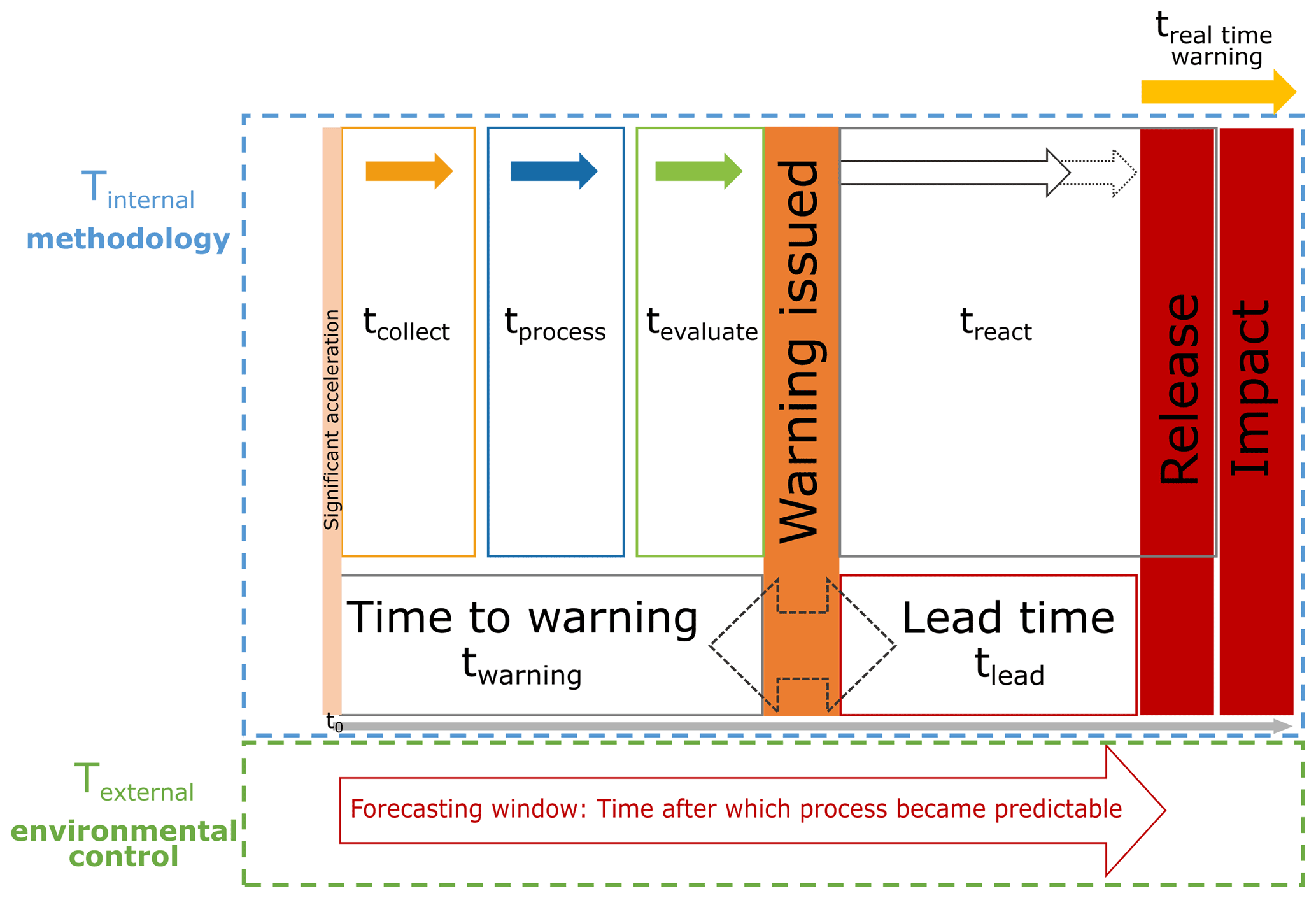
Figure 1The novel conceptual approach for lead time, time to warning and the forecasting window for optical image analysis.
The forecasting window is started (texternal, dashed green outline) following significant acceleration exceeding a set displacement threshold, leading to a continuous process. Simultaneously with the forecasting window, time to warning (twarning) starts (grey outline). Time to warning is divided into a three-phase process to allow time estimations for a comparative assessment of different types of remote sensing data. This process consists of the phases (1) time to collect, (2) time to process and (3) time to evaluate, each with their individual durations. Confidence in the forecasted event increases with time as process acceleration becomes more certain. Once a warning is released (orange box), the lead time begins (tlead) and is terminated by the following release and subsequent impact (red box). The lead time is the difference between the forecasting window and the time to warning. During the lead time, reaction time (treact) starts when appropriate countermeasures are taken to prepare for and reduce risks ahead of the impending event and ends with the final impact.
The time-to-warning period (twarning) is defined by the time necessary to systematically collect data, analyse the available information and evaluate it. Hence, the greater the lead time, the more extensively countermeasures can be implemented prior to the event. An imperative for an effective EWS is that the required time to take appropriate mitigation and response measures has to be within the lead time interval (tlead) (Pecoraro et al., 2019) with tlead≥treact.
2.2 Practical implementation of multispectral data in the concept
The time to warning consists of a three-phase process (see Sect. 2.1 and Fig. 1) to allow rough time estimations for a comparative assessment of different types of remote sensing data. Nevertheless, to realise this temporal concept an established operating system is required, which includes reference data (DEM, previous results); experience from past fieldwork and ready UAS flight plans with preparation for a UAS flight campaign; satellite data access; experience in the single software processing steps including final classification and visualisation templates; and, if utilised for UASs, installed and measured ground control points.
The first phase includes the collection of data starting from the acquisition by the sensor, the data transfer, image pre-processing and provision to the end user. The user selects images online from the data hub and downloads and organises them. For a UAS campaign, the user must obtain flight permits, check flight paths and conduct the UAS flight. The second phase encompasses time to process for the complete data handling from the downloaded data to final analysis-ready image stacks in a GIS or corresponding software. These preparatory steps may include image selection and renaming, atmospheric correction, co-registration, resampling and translation to other spatial resolutions and geographic projection systems, adjustments such as clipping, stacking of single bands into one multispectral image or the division into single bands, and calculation of hillshade from the DEM among others, depending on the requirements. Following this preparation, the data are processed with the appropriate software tools to derive ground motion, calculate total displacement and derive surface changes, e.g. volume calculations or profiles. In the third and last phase, time to evaluate, the results are compared to inventory data and, if available, ground truth data, displacement results of other sensors or different spatial resolutions, and different time interval variations to observe changes in sensitivity to meteorological conditions. Additionally, filters may be applied to eliminate noise. Finally, the results are analysed and evaluated. In each phase quality management is carried out for data access and pre- and post-processing. In time to collect, the images must be selected manually prior to any download from the data hub, as its filter tool options on cloud and scene coverage are of limited help. Accordingly, the areal selection may be misleading as the region of interest (RoI) might not be fully covered, though the sought-after, smaller area of interest (AoI) is covered but not returned from the request. Concerning cloud filters, first, the filter refers to the RoI as a whole in terms of percentage of cloud coverage. The AoI can still be free of clouds or else be the only area covered by clouds in the total RoI. Therefore, an image is either not returned although usable or returned but not useable. Second, clouds can create shadows for which no filter is available. As a result, affected images have to be manually removed by the user. Images which are of low quality due to snow cover have to be discarded too. These actions indirectly represent the first quality checks in the collection phase. In the following processing phase, the images in a GIS are checked for quality and accuracy. Depending on the data provider, some pre-processing such as radiometric, atmospheric and/or geometric corrections may be conducted. During this phase, additional user-based steps will be checked if necessary. Finally, the results are compared to other data (e.g. DEM, dGPS), are reviewed for their validity and may be supplemented by statistical evaluation.
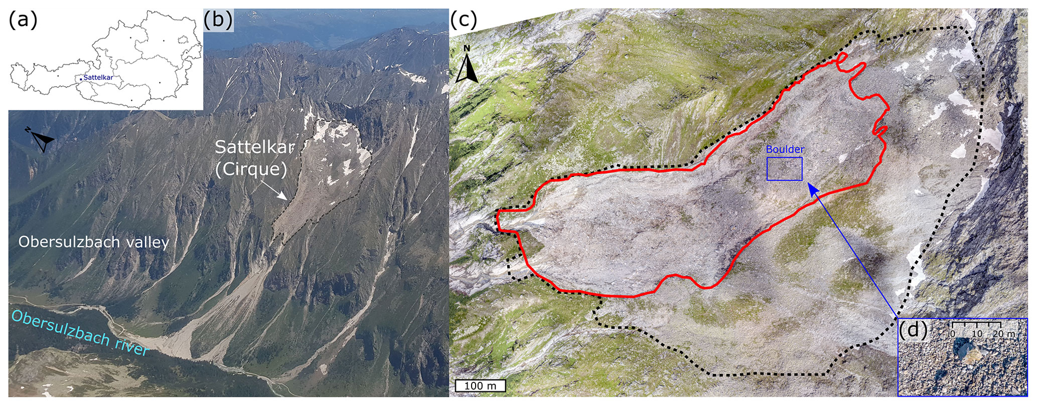
Figure 2In August 2014, heavy ongoing precipitation triggered massive debris flow activity of 170 000 m3 in volume, of which approximately 70 000 m3 derived from the catchment above 2000 m. A further 100 000 m3 was mobilised in the channel within the cone. The consequence was that the river Obersulzbach was blocked, leading to a general flooding situation in the catchment and resulting in substantial destruction in the middle and lower reaches (Fig. 3).

Figure 3Obersulzbach valley, flood event September 2014. (a) Flooding situation in the Obersulzbach valley with the Sattelkar landslide cone deposit (image centre). (b) Flood area at the valley mouth in Sulzau and Schaffau. The river Salzach is at the bottom of the image. © Salzburger Nachrichten/Anton Kaindl.
The Sattelkar is a steep, high alpine, deglaciated, west-facing cirque at an altitude of between 2130–2730 m a.s.l. in the Obersulzbach valley, Großvenedigergruppe, Austria (Fig. 2a). Surrounded by a headwall of granitic gneiss, the cirque infill is characterised by massive volumes of glacial and periglacial debris as well as rockfall deposits (Fig. 2b, c). Since 2003 surface changes have taken place as evidenced by a massive degradation of the vegetation cover and the exposure and increased mobilisation of loose material. A terrain analysis revealed that a deep-seated, retrogressive movement in the debris cover of the cirque had been initiated (Anker et al., 2016; GeoResearch, 2018). High water (over)saturation is assumed to be causing the spreading and sliding of the glacial and periglacial debris cover on the underlying, glacially smoothed bedrock cirque floor, forming a complex landslide (Hungr et al., 2014). Detailed aerial orthophoto analyses, witness reports and damage documentations indicate a steady increase in mass movement and debris flow activity over the last decade (Anker et al., 2016).
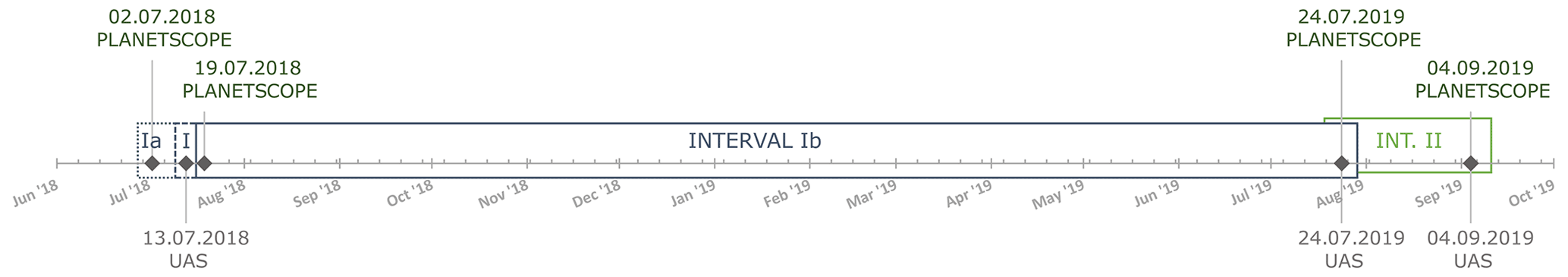
Figure 4Acquisition dates of UAS and PlanetScope images within the investigated time period. Calculated interval I for UAS images (13 July 2018–24 July 2019, 376 d) and interval Ib for PlanetScope images (19 July 2018–24 July 2019, 370 d) and interval II for UAS and PlanetScope images (24 July–4 September 2019, 42 d). Note that the Ia PlanetScope interval was discarded.
The Sattelkar has been the focus of international research projects such as PROJECT Sattelkar (GeoResearch, 2018) and AlpSenseBench (TUM, 2020) since 2018. In 2015 preliminary findings revealed a mass movement coverage of 130 000 m2 with approximately 1×10⁶ m3 of debris and displacement rates of more than 10 m yr−1. The debris consists of boulders up to 10 m in diameter (Fig. 2c, d), allowing visual block tracking and delimiting the active process area. High displacement was measured between 2012 and 2015 with up to 30 m yr−1.
In the Sattelkar cirque, several monitoring components are installed to provide ongoing and long-term monitoring. Nine permanent ground control points (GCPs) are measured with a dGPS to provide stable and optimal conditions to derive orthophotos from highly accurate UAS images (GeoResearch, 2018). A total number of 15 near-surface temperature loggers (buried at 0.1 m depth) recorded annual mean temperatures slightly above the freezing point (1–2 ∘C) in the period 2016 to 2019. Ground thermal conditions at depth react with significant lag times to recent warming and therefore are primarily determined by climatic conditions of the past (Noetzli et al., 2019). Significantly cooler climatic conditions in previous decades and centuries (Auer et al., 2007) thus likely contributed to the formation of (patchy) permafrost at the Sattelkar cirque. Recent empirical–statistical modelling of permafrost distribution in the Hohe Tauern Range confirms possible permafrost presence at the study site (Schrott et al., 2012).
The Sattelkar is a suitable case study as it is in the early stages of the landslide development and thus fits best to this conceptual approach. Here, processes take place on timescales appropriate for long-term observation to provide sufficient warning time. The active part of the cirque has accelerated in recent years, allowing the analysis of EWS concepts based on multispectral optical remote sensing data supported by complementary block tracking.
4.1 Optical imagery
Optical satellite imagery is more appropriate for high-deformation studies than radar applications are due to its high spatial resolution as well as the short time span between acquisitions (Delacourt et al., 2007). Although the west-facing slope is favourable for the application of radar derivatives (InSAR/DInSAR), the choice to use optical imagery is based on the observed high displacement rates, which cause decorrelation when using radar technologies as they are more sensitive than optical technologies. Complex and/or large displacement gradients make the phase ambiguity difficult to solve for radar interferometry (Kääb et al., 2017). Revisit times of current radar satellites (e.g. Sentinel-1) are longer than those of optical satellites, and if time periods between image acquisition become too long, ground motion may accumulate such that the displacement is too high to be measured. Several studies on displacements of faults and landslides have shown the potential of optical data to provide detailed displacement measurements based on image correlation techniques (DIC) (Leprince et al., 2007; Rosu et al., 2015). A further advantage of optical images for geomorphological processes in steep terrain is their viewing geometry (close to nadir) (Lacroix et al., 2019). Here we employ DIC to compare the spatiotemporal resolution of multispectral optical imagery (UAS and PlanetScope) and to assess its suitability for early warning purposes. UAS images offer excellent spatial resolution and accuracy at the centimetre scale (Turner et al., 2015) and complement large-scale satellite or airborne acquisitions (Lucieer et al., 2014). PlanetScope imagery provides the highest temporal resolution among available sensors with daily acquisitions, guaranteed data availability, and free and open access for research purposes. In this study the PlanetScope Analytic Ortho Scene SR (surface reflectance) imagery (16 bit; geometric, sensor and radiometric corrections) was employed (Planet Labs, 2020b) and was supported by the Planet Labs Education and Research Program.
4.2 Data availability of PlanetScope
Research on the availability and usability of PlanetScope imagery was conducted on the Planet Explorer data hub for the time span from the beginning of April to the end of October in 2019, as during these months snow cover should be negligible. Filter parameters were solely set for four-band PlanetScope Ortho Scene data and the Sattelkar AoI. In order to obtain all available images, no filters (e.g. sun azimuth, off-nadir angle) were applied. We defined four categories: (i) meteorological constraints due to snow cover, cloud cover and cloud shadow; (ii) image (coverage) errors made by the provider, (iii) no data availability; and (iv) the remainder of usable data (Table 2). The output request was evaluated according to the defined categories and was compared to the provider's guaranteed daily image provision, which is comprised of 213 d for the time period (1 April–31 October 2019). We calculated percentages for the above categories based on days per month as well as a 7-month sum and percentage average. The availability analysis did not include an examination of the data with regard to their spatial usability in terms of their positional accuracy and/or image shifts.
Table 2PlanetScope four-band data availability and usability for Sattelkar AoI for April to October 2019.
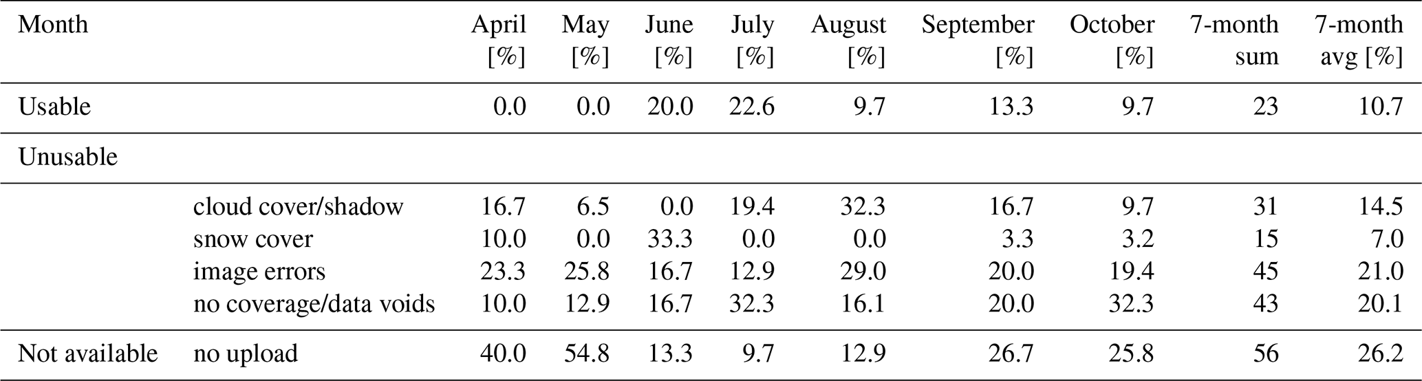
Unfavourable meteorological influences of cloud cover/shadow and snow cover affected up to 32.3 % and up to 33.3 %, respectively, on all 213 d; on average 14.5 % and 7 % of the days were not usable (Table 2). For 10 d in June snow influence had the greatest negative share (33.3 %); for April there was 3 d of snow coverage, and the months September and October each had 1 d of snow coverage. Cloud cover/shadow exerted a higher impact on data usability by 14.5 %. Problems on the part of Planet Labs made many of the data unusable due to image errors: between four and nine images per month were not usable (21 %). On average for 26.2 % of the analysed time period no image data were available. In this 7-month period, 43 images (20.1 %) had data voids or did not cover the AoI; thus the overall usability is limited to about 11 %.
4.3 Data acquisition and processing
In line with the concept in Fig. 1 (Sect. 1), the following processing steps are categorised and described.
-
tcollect. UAS data acquisition was preceded by detailed flight route planning and checks of local weather and snow conditions. UAS flights were carried out with a DJI Phantom 4 UAS on 13 July 2018, 24 July 2019 and 4 September 2019 (see Table 3; Figs. 4, 6b, c).
For each acquisition, the total area was covered by four flights which were started at different elevations (Table 4). Flight planning was carried out with UgCS maintaining a high overlap (front 80 %, side 70 %) and a target ground sampling distance (GSD) of 7 cm. The area covered was approximately 3.4 km2, and with a flight speed of about 8 m s−1 total flight time took 3.5 h. The images were captured in RAW format. In the Planet Explorer data hub, PlanetScope Ortho Scene data were selected for usability; imagery affected by snow cover, cloud cover, cloud shadow and partial AoI coverage was discarded (Table 5).
-
tprocess. In phase two (time to process) the PlanetScope images were visualised in QGIS. Thereafter, a second selection (visually with the MapSwipe Tool plugin) from the downloaded images was filtered for errors of location, inter-tile shift and shifts in the individual bands which were previously not clearly discernible in the online data hub. The final selection of images was made based on the temporal proximity to the UAS data to guarantee the best comparability. For acquisition set (1), there are two PlanetScope images (2 and 19 July 2018) which differed from the UAS acquisition date (13 July 2018) by 11 and 6 d, respectively. For acquisition sets (2) and (3), PlanetScope and UAS acquisition dates were identical (24 July and 4 September 2019). The acquired datasets were categorised into chronological intervals I, Ia, Ib and II (see Fig. 4).
The UAS images in RAW format were modified using Adobe Exposure to improve contrast, highlights, shadows and clarity. Thereafter, they were exported as JPG files (compression 95 %) and processed with PIX4Dmapper to a 0.08 m resolution and orthorectified based on nine permanent ground control points (GCPs, 30×30 cm). These were repeatedly (1000 measurements/position) registered with the Trimble R5 dGPS and corrected via the baseline data of the Austrian Positioning Service (APOS) provided by the BEV (Bundesamt für Eich- und Vermessungswesen). Horizontal root-mean-squared errors (RMSEs) range from 0.05 to 0.10 m for vertical RMSE. These GCPs were employed for georeferencing and further rectification of all UAS surveys.
Next, the data were clipped to a common area of interest (AoI) and resampled with GDAL and the cubic convolution method to 0.16 m to enhance processing time and increased reliability of image correlation. PlanetScope Satellite images were co-registered in MATLAB relative to a reference image (https://gitlab.lrz.de/tobi.koch/satelliteregistration.git, 25 February 2021). A feature point detection step was applied to estimate a geometric similarity transformation between the reference (master) and all target (slave) image pairs excluding the AoI with its terrain motion. Thereafter feature point outliers were statistically removed (RANSAC) and the similarity transformation of the slave images to the master image was performed. After removing the outliers, more than 500 feature matches were found for the entire image pair dataset. The mean distance of transformed inlier feature points from the target image to their corresponding feature matches in the reference image ranged between 0.6 and 0.8 pixels, confirming the high registration accuracy (see Fig. S14 in the Supplement). We used digital image correlation (DIC) to measure the displacement for the active landslide body of the Sattelkar and to assess the suitability of the PlanetScope and UAS data. This method employs optical and elevation data and calculates the distance between an image pair, based on the spatial distance of the highest correlation peaks between an initial search and a final reference window. The result provides displacement and ground deformation in 2D on a sub-pixel level. COSI-Corr (Co-registration of Optically Sensed Images and Correlation), widely used software in landslide and earthquake studies, was used for sub-pixel image correlation (Stumpf, 2013; Lacroix et al., 2015; Rosu et al., 2015; Bozzano et al., 2018). COSI-Corr is an open-source software add-on developed by Caltech (Leprince et al., 2007), for ENVI Classic. There are two correlators: in the frequency domain based on an FFT (fast Fourier transformation) algorithm and a statistical one. Applying the more accurate frequential correlator engine, recommended for optical images, different parameter combinations of window sizes, direction step sizes and robustness iterations were tested. Parameter settings include the initial window size for the estimation of the pixelwise displacement between the images and the final window size for sub-pixel displacement computation in x, y; a direction step in x, y between the sliding windows; and several robustness iterations (Table 6). We utilised recommended window sizes as suggested by Leprince et al. (2007) and Bickel et al. (2018). Step size one showed good results while keeping the original spatial resolution for the output; robustness iterations of two to four were sufficient for our purposes. Initial and final window sizes were systematically tested (see Table 6). For computing, a state-of-the-art power station was employed (AMD Ryzen 9 3950X 16-core processor, 3.70 GHz, 128 GB RAM).
The results of each correlation computation return a signal-to-noise ratio (SNR) map and displacement fields in east–west and north–south directions. These results were exported from ENVI Classic as GTiff files, and the total displacement was then calculated with QGIS.
-
tevaluate. In the last phase (time to evaluate) the results of various parameter settings were compared in QGIS and ArcGIS along with different combinations of visualisation. Displacement below a 4 m threshold was discarded from the PlanetScope datasets due to aberrant values (noise, outliers). The threshold definition was defined on (i) the value distribution in both the total displacement and the corresponding SNR result and (ii) a visual comparison of the maps for the total displacement and the SNR. This definition allowed us to identify outliers and unlikely displacement. Apart from this threshold no other filters were employed, and we kept the output raw (see Fig. S13, for raw DIC on PlanetScope). Very few inconsistencies were present in the UAS-derived displacement results, which were accepted without modification.
Additional analyses were performed to estimate the DIC outputs of both the UAS orthophotos and PlanetScope satellite imagery. Visual tracking of 36 single blocks, identifiable in the UAS orthophoto series, allowed deriving direction and amount of movement; this supported the confirmation process for (i) the total displacement and (ii) the results of automated and manual tracking. In the next section we present this approach only for time interval II.
Table 3Acquisition dates of UAS and PlanetScope images, in chronological order.
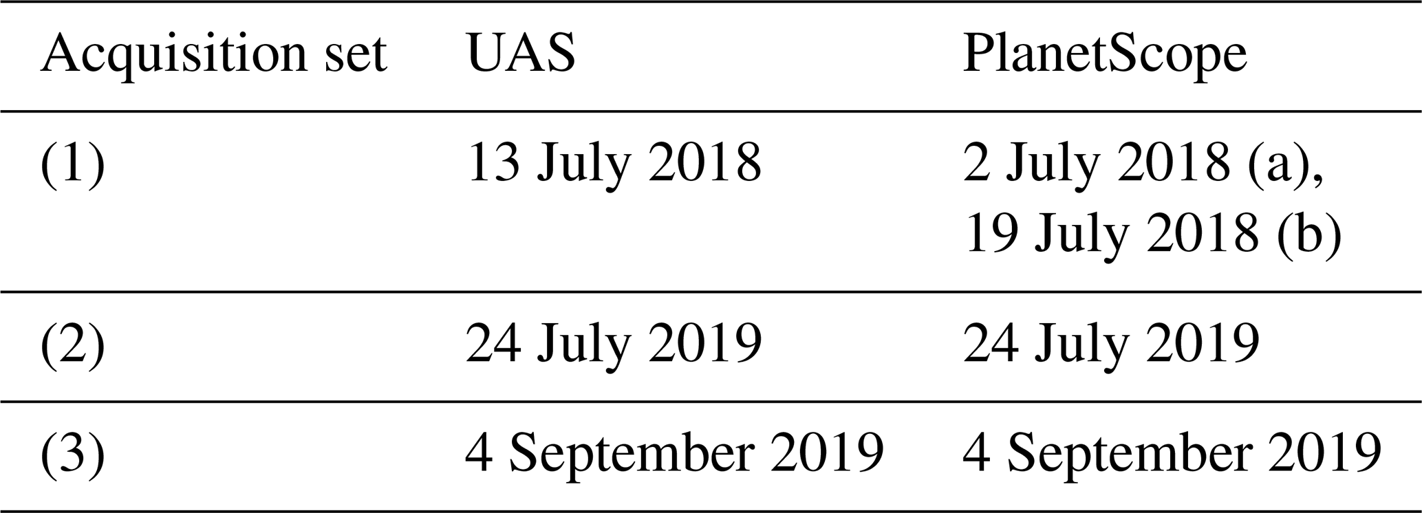
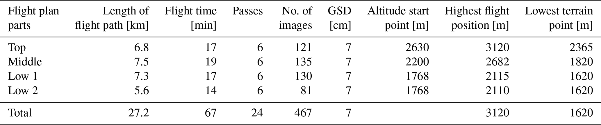
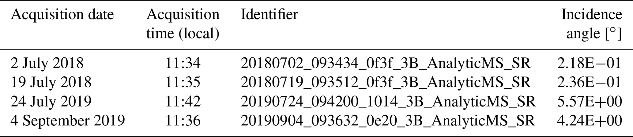
Table 6COSI-Corr input parameters for intervals of the UAS and PlanetScope.

Table 7Relevant dates for historic failures of Vajont (ITA), Preonzo (CH) and the Sattelkar (AUT). Time period in italics–bold used for Fig. 8. Time intervals in days (∼ for rough estimations) and years in square brackets; sum of days based on the first day of the month if only month as reference is available from the literature (Petley and Petley, 2006; Anker et al., 2016; Sättele et al., 2016; Loew et al., 2017). When only the month is given, dates are in the format month/year; when the day is also given, dates are in the format day.month.year. Further explanation is in the text.

In Sect. 5.1 we present ground motion results from DIC for the original input resolution for (i) the UAS, 0.16 m input resolution, and (ii) PlanetScope, 3 m input resolution, based on parameters in Table 6. In Sect. 5.2 DIC results for the UAS, 0.16 m, are analysed with regard to displacement of visual single block tracking. Finally, in Sect. 5.3 required times for tcollection, tprocessing and tevaluation for each sensor are presented.
5.1 Total displacements

Figure 5Results of DIC total displacement of orthoimages for the UAS for (a) and (b) at a 0.16 m resolution and PlanetScope (c) and (d) at a 3 m resolution. Time intervals for UAS image pair (a) I (13 July 2018–24 July 2019, 376 d) and (b) II (24 July–4 September 2019, 42 d) and for PlanetScope (c) Ib (19 July 2018–24 July 2019, 370 d) and (d) II (24 July–4 September 2019, 42 d). Explanation of inconsistently tracked features (a) a and b and (b) b and the northwestern landslide head are described in Sect. 5.2. The solid black line represents the boundary of the active landslide based on field mapping. Background: hillshade of lidar DEM, 1 m resolution (© SAGIS).
Figure 5a and b show the total displacements derived from UAS orthophotos at a 0.16 m resolution for time intervals I and II (see Table 6). Apart from several minor displacement patches, no motion is visible outside the active body in either period. Time interval I (376 d) (Fig. 5a) shows mean displacement values from 6 to 14 m for a coherent area in the eastern half of the lobe from the centre (c) to the eastern boundary of the active area. The highest displacement rates (up to 20 m) are observed within small high-velocity clusters in the northwest section (d). Lower velocities occur along the southern boundary (e,f), ranging from zero to 6 m with smooth transitions. Ambiguous, small-scale patterns with highly variable displacement rates are present in the western half (a) and along the northern boundary (b). No motion is detected along the western fringe (i.e. at the landslide head) which is 20 m in width. South of the landslide (g) there is a small patch of minor displacement with continuous (up to 3.5 m) and ambiguous signals. Furthermore, we observed small-scale patterns of ambiguous signals in the east (j) and in the west of the active area in the drainage channels (h,i).
Time interval II (42 d) (Fig. 5b) shows great similarity to time interval I with ambiguous signals in the same areas such as the drainage channels (h, i) and within the western half of the active area (b). In contrast to interval I (Fig. 5a), within the active area a homogenous higher-velocity patch (up to 6 m) near the landslide head is evident (a). In the eastern half large homogenous patches extend from the landslide centre (c) to the root zone (d), showing coherent displacement values of zero to 4 m. During this shorter time interval II, no displacement is detected along the southeastern boundary (e) and for large parts of the root zone (f) previously covered in I. Similarly to I, the landslide head has a 20 m rim free of signal (see also x and y in Fig. 6). In the central part of the lobe (c) total displacements are significantly reduced.
Figure 5c and d demonstrate total displacement for similar time intervals to those of the UAS (see Table 3 and Fig. 4). For interval Ib (370 d) (Fig. 5c) wide fringes with no motion were detected around an actively moving core area, which consists of small-scale clusters with variable total displacement in the western part, coherent high velocities in the middle and coherent low velocities east of this core area. Outside the landslide, northeast and immediately south (j), high-velocity patches are observed.
In interval II (42 d) (Fig. 5d) the detected displacement is restricted to the western half of the landslide (a) and shows the same significant fringes with no motion as in I. Compared to interval I the motion pattern of this core area is more homogeneous with increasing displacement towards the east. Outside the active area several patches show medium to high total displacement, the largest of which is located 300 m northwest of the landslide (i).
5.2 Single block tracking
Figure 6a illustrates the total displacement derived from the UAS data at a high resolution (0.16 m) for interval II (42 d). UAS orthoimages were used to manually measure single block displacement for 36 clearly identifiable boulders on the landslide surface. Block displacements of 1 m are visible in the eastern part (f), whereas DIC does not reveal any displacement below 1 m. Boulder tracks longer than 2 m in the central and western part of the landslide are reflected by DIC-derived displacement values. Near the front a 6 m displacement of one block (a) is represented in the DIC result. The highest values (6, 10 and 16 m) were observed in regions where DIC delivered ambiguous, small-scale patterns of highly variable displacements. Displacement vectors show consistent bearings in the downslope direction of the landslide motion for homogeneous areas of the DIC result (a, c, d); there are short vectors with chaotic bearings in areas of ambiguous patterns (b), some of which are pointing upslope. The vectors show no displacement in stable areas outside the active area and where no DIC signal is returned.
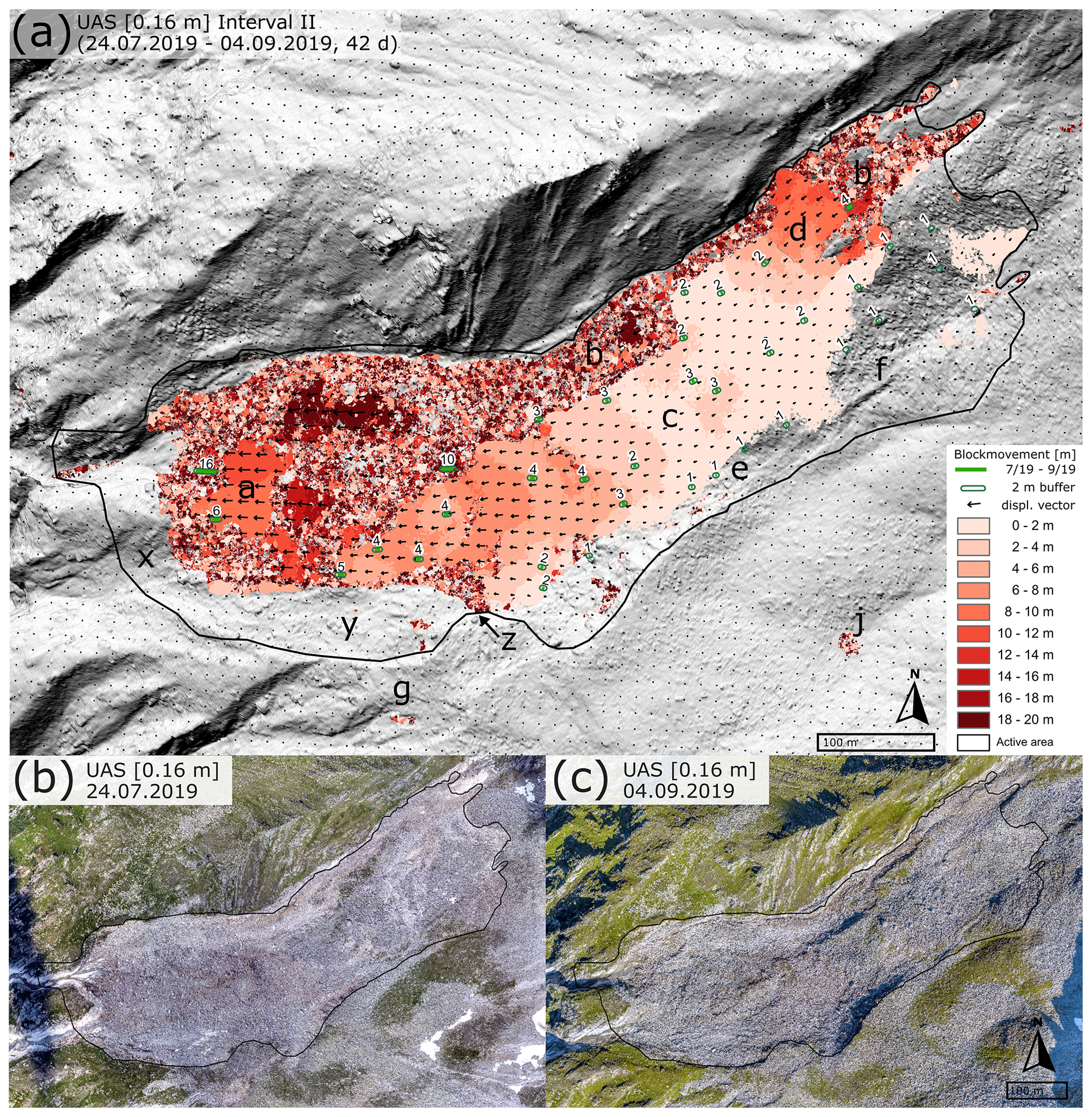
Figure 6(a) Displacement derived from UAS data at a 0.16 m resolution for interval II (24 July–4 September 2019, 42 d) combined with boulder trajectories (in metres) manually measured in the UAS orthophotos in the same time period. Displacement vectors show landslide flow (black). Origin of inconsistently tracked features (a) for b and the northwestern landslide head are described in Sect. 5.2. The solid black line represents the boundary of the active landslide based on field mapping. Background: UAS hillshade, 24 July 2019 (0.08 m), orientation −3∘ from north. UAS orthophotos at a 0.16 m resolution for the master (b) and slave image (c) of the corresponding time interval.
5.3 Time required for collection, processing and evaluation
In Sect. 2 we introduced a novel concept to extend lead time, consisting of three phases within the warning time window (see Fig. 1). This concept is based on DIC results; thus every step comprised in each phase has been previously undertaken. On this basis, knowledge of required time for a further process iteration of the three phases is given.
The time required for collection, processing and evaluation of UAS and PlanetScope data is estimated and summed in Fig. 7. Planet Labs specifies 12 h from image acquisition to the provision in the data hub, which includes to a large extent data pre-processing (Planet Labs, 2020b). Adding 2 h for the selection, ordering and download process, we assume that the time required for the collection phase is approximately the same for both sensors, with 14 h for PlanetScope and 12 h for the UAS. With regard to the time needed for the processing phase, the sensors differ with the UAS requiring 17 h and PlanetScope 5 h. Time for the evaluation phase is estimated to be about 2 h. In sum, twarning for the UAS is approximately 31 h compared to 21 h for PlanetScope.
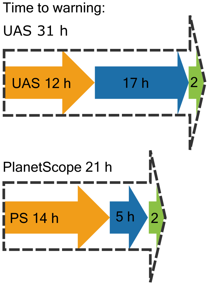
Figure 7Time to warning is composed of three phases: time to collect, to process and to deliver. Time to warning (subsequent to acceleration) is 21 h for PlanetScope and 31 h for the UAS. Thus, any hazard process that takes longer than 21/31 h to prepare the release and impact can be forecasted.
To systematically analyse the predictive power of the UAS and PlanetScope data, we will (i) evaluate ambiguous signals, error sources and output performance; (ii) assess obtainable temporal and spatial resolutions; and (iii) derive a systemic estimate of the minimum obtainable warning times.
6.1 Error sources and output performance
To evaluate error sources and output performance, we compared results of digital image correlation results from optical data with (i) high-resolution UAS orthophotos, (ii) mapped mass movement boundaries and (iii) visual block tracking for UAS orthophotos. The approximately 1-year evaluation period encompassed all seasons; hence freezing–thawing conditions and a wide range of meteorological influences, e.g. thunderstorms and heavy rainfall, are included. The two investigated time intervals are I/Ib and II, covering 376/370 and 42 d (typical high alpine summer season), respectively (Fig. 4). Interval II exclusively covers (high alpine) summer conditions, with negligible to no contribution from freezing conditions. As these inclusion periods are inconsistent, the amount of total displacement cannot be directly compared; however the relative motion patterns can be. Accordingly, we can confirm the suggested parameter settings of earlier studies on window sizes, steps and robustness iterations (Ayoub et al., 2009; Bickel et al., 2018).
In terms of the mass movement boundary, the total displacement derived from the DIC of the UAS data generally matches the field-mapped landslide boundary for both intervals (I, II) (Fig. 5a, b) and is supported by the absence of significant noise outside the AoI. Mapped boulder trajectories for interval II (see Fig. 6) are consistent with the calculated total displacement and thus confirm COSI-Corr as a reliable DIC tool to derive ground motion for this study site and UAS orthophotos as suitable input data. Nevertheless, there are several areas with ambiguous signals. Here we follow Leprince et al. (2007) describing a correlation loss as “decorrelation” with signal-to-noise values that are low/null (i.e. no convergence of the correlation algorithm) and/or large offsets, which are either unrealistic in nature or beyond the valid matching window distance. Decorrelation in our understanding exhibits a salt-and-pepper appearance in the DIC result with random displacement vectors, related to inconsistently tracked features. The software is not able to find the corresponding, correlated surface pattern, leading to a misfit (i.e. misrepresentation) and/or mismatch (i.e. blunders) of the matching windows and finally resulting in noise (Debella-Gilo, 2011; Guerriero et al., 2020). Nevertheless, this decorrelation signal is still a valuable observation that might be related to surface processes and not only to erroneous limitations of the DIC method. There are four main reasons that might cause these effects: (i) significant temporal change of the surface, i.e. revolving and/or rotational deformation; (ii) high displacements exceeding the matching window size being smaller than the offset; (iii) land cover changes such as snow cover, vegetation cover and alluvial processes; and (iv) changes related to illumination (e.g. shadow) or image errors (e.g. orthorectification, shifts in individual bands) (Leprince, 2008; Debella-Gilo, 2011; Lucieer et al., 2014; Stumpf et al., 2016). In our study, the decorrelated salt-and-pepper areas include to a large degree the landslide head (a), the drainage channel (h) (Fig. 5a, b), a larger patch south of the active area boundary (g) (Fig. 5a), and some smaller patches in little depressions (g) (Fig. 5a) and (j) (Fig. 5a, b). The patches j and east of j are identified as snow fields in the orthophotos and the noise results from decorrelation. In Fig. 5a, the large southern patch (g) shows clear displacement values for the rear part and decorrelation for the front region resulting from morphological changes within the image pair of interval I (see Fig. S12). This is due to a gain of between 1 and 2 m for an area of about 250 m2. The decorrelation in the drainage channel (h) could stem from massive changes in pixel values, similarly to the decorrelation on the basis of alluvial processes, as described by Leprince et al. (2007). Decorrelations in the areas with the fastest ground motions also lead to high pixel changes (Stumpf et al., 2016): these are observable in the active landslide area within the lobe, where large areas of decorrelation may be explained by high displacements in the leading landslide head (a) with re-detected, hence correlated, pixels in the trailing areas (c, d, e, f). These findings can be transferred to the landslide interior area (a, b) and the frontal western regions and the northern margin (b). The observation is confirmed by geomorphological mapping (see Fig. S11) and measured boulder block trajectories from the orthophotos (Fig. 6a). Several patches of correlation (c, f) with corresponding boulder trajectories of up to 4 m (34.8 m yr−1) (d) can be detected in the rear areas. A correlated patch with a 16 m (34.8 m yr−1) trajectory (a) is located in the flow direction behind the foremost boulder. In this case the method was able to partially capture the displacement as the distinct boulder block supported the detection, which probably led to correlation. Similarly there is another example with a trajectory of 10 m (86.9 m yr−1) outside a homogeneous correlated area. This leads to the assumption that for the calculated time period, with 63 pixels or more at a resolution of 0.16 m, no pixel matching is possible and probably reached the correlation capacity due to the too-high displacement. With a correlation window smaller than the displacement, the algorithm cannot capture the displacement (Stumpf et al., 2016). However field observations provide evidence that the rock masses are deforming, and the surface is altering due to the high mobility and rotational behaviour of some boulder blocks. This leads to changed pixel values and spectral characteristics of the block surface and the surrounding area, which can also result in poor correlations and even random errors and mismatches (Debella-Gilo and Kääb, 2011). This finding is similar to observations in a rock glacier study by Debella-Gilo and Kääb (2011). Similar results were observed by Lucieer et al. (2014), who described a loss of recognisable surface patterns if revolving and rotational displacements occur, causing decorrelation and noise as output. These results show that with COSI-Corr and UAS orthophotos of 0.16 m, it is possible to detect the total displacement of the landslide in both extent and internal process behaviour even in this steep, heterogeneous terrain. Nevertheless, high displacement rates and rotational surface behaviour in the cirque limit the DIC method. A decrease in the time interval for this particular highly mobile study site would likely reveal an enhanced correlation since for shorter time periods the total displacement decreases and surface changes are reduced, which can be controlled by shortening the temporal baseline (Debella-Gilo and Kääb, 2011). In sum, though the results contain heterogeneous, noisy, decorrelated areas, the combination with homogeneous displacement areas still offers valuable insights into this and other internal landslide structures and complex behaviours.
6.2 Comparison of temporal and spatial resolution
We compared the COSI-Corr total displacement results of PlanetScope (Ib and II; Fig. 5c, d) and UAS images (I and II; Figs. 5a, b and 6a) for the same time periods at different spatial resolutions (see Table 6). For the PlanetScope DIC result the main part of the landslide is detected, and its area is generally consistent with the results of the UAS DIC, which is additionally confirmed by boulder trajectories. The frontal part (a) reveals correlation signals (I and II), while for the same time intervals and parts, the UAS DIC results show a decorrelation (Ib and II). The correlation is likely to be attributable to the coarser spatial resolution of 3 m PlanetScope input data and hence a smaller number of pixels to be captured at this site with the DIC method. Similar texture of rock clast surfaces could lead to false positives resulting in correlation as patches appear to be similar in matching windows. However, in contrast to the UAS result (Fig. 5a, b), the outcome on a large scale fails to detect the entire actual active area (b and f) as well as its internal motion behaviour. Nevertheless, for the visualisation and analysis of the PlanetScope results, the range of total displacements had to be restricted to values equal to and greater than 4 m due to noise and outliers over large areas, as applied and described by Bontemps et al. (2018). Even then, noise and several misrepresented displacement patches are observed for i and j and in the northeast image corner (Fig. 5). We can identify several reasons for these large clusters of high motion values. Massive cloud and snow coverage hampered the first images of both interval Ib (19 July 2018) (Fig. 5c) and interval II (24 July 2019) (Fig. 5d), leading to a 20 m fringe of false displacements in the northeastern part of the image. Minor snow fields as visible in the images from 24 July 2019 for both the UAS and PlanetScope likely explain the big cluster of incorrect displacements southeast of the lobe (j); nonetheless, in the satellite image they are smaller than the resulting DIC displacement. High cloud coverage in two input images with large areas of white pixels may exert an influence leading to high gains due to sensor saturation (Leprince, 2008). Illumination changes in interval II (Fig. 5d) may cause unrealistic displacements outside the boundary with slightly darker colours due to shadows in the first satellite image (24 July 2019), and large parts within the second image (4 September 2019) are also in the shade. A comparison of the acquisition times and true sun zenith, e.g. for the second image, reveals a difference of 1 h 34 min between the image acquisition at 11:36 LT (local time) and the true local solar time at 13:10 LT. As the study site is located in a high alpine terrain with a west-facing cirque, at this time of day there are shadows of considerable length which have a significant influence on the result of digital image correlations. One clear advantage of the UAS images is that their acquisition is plannable according to the best illumination conditions with the sun at its zenith. Moreover, the UAS flight path as well as the system itself remained the same for all three acquisitions, while PlanetScope employs various satellites.
Despite different input resolutions and time intervals (Ib vs. I and II vs. II; see Table 3) with different sensors (UAS, PlanetScope), there is a similarity for the landslide head which indicates that the displacement is restricted to a smaller area than the previously demarcated boundary, based on our field investigations. This is clearer for the time interval I (376/370 d) (Fig. 5a vs. c) as for the longer temporal baseline the total displacement accumulation is higher and thus better captured by COSI-Corr for PlanetScope with a 3 m resolution. Due to the shorter interval II (42 d) (Fig. 5b vs. d) with less accumulated total displacement, the rear of the landslide is not represented; no signal is shown as the total displacement for PlanetScope was restricted to values above 4 m. Values below 4 m had to be discarded for PlanetScope DIC results as they were lost in noise; i.e. for the entire DIC results there is total displacement of between 0 and 4 m (see Fig. S13). Hence, when applying a minimum threshold of 4 m, the satellite image detects large parts of the main active core area, but widths of 50–80 m from the boundary show no displacement. However, large false clusters of high total displacement are within the PlanetScope result for interval I for j and the northeast image corner (Fig. 5c) and interval II for i (Fig. 5d).
Measured ground motion of block tracking and PlanetScope results indicate and support existing high ground motions. In addition there are morphologically significant volumetric turnovers with areas of large gains and losses of ±5 m (see Fig. S11). These observations might explain the resulting decorrelation at the finer resolution of 0.16 m for the landslide head: the matching window is smaller than the offset and texture surface changes are too complex to be re-detected, i.e. matched, and thus correlated, leading to decorrelation and noise. Homogeneous correlated patches are at the front of the landslide body for the shorter time interval; there may have been some displacement just below the detection threshold for this high ground motion, or some boulders and their surroundings might have been matched, or both may apply (Fig. 6a, a). In this case for the complex ground motion with high-spatial-resolution data, the previous assumption based on a shorter time interval likely leads to improved detection of inherent process behaviour (see Sect. 6.1). Generally, with high-resolution images, such as those of UASs, we recommend first calculating displacements based on a coarser input resolution (1–3 m) to examine the overall situation and detect changes and second calculating displacements at a finer resolution in order to focus on relevant details of the AoI. With regard to PlanetScope data, a 3 m resolution seems to be in a good spatial range to assess ground displacements even of this steep and heterogeneous study site with its high motion. Nonetheless, constraints such as illumination due to early daytime acquisitions leading to shadows and meteorological influences by clouds, cloud shadows and snow decrease the quality of the satellite images and reduce their applicability. Sensor saturation, shadow length, size and direction as well as changes in snow, cloud or vegetation cover impose limitations (Delacourt et al., 2007; Leprince et al., 2008) and accord with our observations. The authors identify additional limitations such as radiometric noise, sensor aliasing, human-made changes and co-registration errors (Leprince et al., 2008). All these limitations have a negative impact on the input image, which leads to impaired DIC calculations and results and (partially or wholly) inaccurate analysis of the displacement. These limitations might have played a role in our results. In our experience, the usability of the DIC result may be influenced by the input image quality. This restricts the application of PlanetScope images to a certain degree. They can be employed as input data to detect displacements, but as there are in the present setting too many signals of false-positive displacements, which can be discarded solely on the basis of field evidence, these data are currently of limited use. They should be handled with caution, and we recommend combining them with complementary data and ground truth.
6.3 Estimating time to warning
Early warning is essentially defined as being earlier than the event and thus puts high external time constraints on observation and decision. The time window between the detection of an accelerating movement and preparing for final failure and the final failure itself is determined by the environment. Therefore, two sensors with the highest-available spatiotemporal resolution were evaluated and compared with regard to their applicability to the early warning of landslides. We made rough assumptions and assessed the time needed for the phases of time (i) to collect, (ii) to process and (iii) to evaluate relevant data (summarised in the time-to-warning window; see Fig. 7).
Despite different underlying technologies, the time required for the collection phase is approximately the same for both sensors. For the UAS, we estimated about 12 h under ideal circumstances, while for PlanetScope we estimated 12 h (Planet Labs, 2020b) plus 2 h for image selection, download and initial analysis, adding up to 14 h in total (see Sect. 5.3). In the second phase, time to process, deriving orthophotos from raw UAS images is time consuming. The subsequent DIC calculations demand significantly more processing time for the UAS images than for lower-resolution PlanetScope images. The final phase, time to deliver, takes about 2 h for each sensor. In our case study, the estimated time to warning (twarning) was 10 h longer for the UAS approach (31 h) in comparison to the PlanetScope approach (21 h). These time calculations are based on ideal environmental conditions and data availability. Assuming good conditions exist to conduct the UAS flight and no constraints limit the utilisation of satellite images, in theory a daily deployment is possible. In reality, unfavourable weather conditions and cloud and snow cover as well as limited data availability will increase the actual twarning significantly. From the available images in the Planet Data hub (besides other exclusions) meteorological influences reduced for April–October 2019 the usability to 14.5 % and 7 % for cloud cover and snow cover, respectively (Table 2). The flexibility of a UAS can serve as a practical remote sensing tool for the investigation of ground motion behaviour in a spatiotemporal context. Nonetheless, weather influences can make a UAS flight impossible or impractical as the result might be useless. Depending on the level of illumination, the same may apply for satellite images. Regardless of any meteorological constraints, the promised daily availability by PlanetScope is unrealistic, due to data gaps and provider issues; our study showed that for the Sattelkar from April to October 2019 only 11 % of the captured images during this time were usable. Hence, PlanetScope data have a temporal availability that is similar to Sentinel-1 with a 6 d revisit time. In time-critical early warning scenarios, when time is running out, all available even partly usable images will be utilised and fieldwork may be conducted, even if the prevailing conditions are suboptimal but will increase data availability. The comparison of two selected remote sensing options demonstrates that comprehensive knowledge of the available remote sensing data sources and their respective time requirements can substantially reduce the time to warning (twarning) and extend the lead time (tlead).
Significant observations of the temporal evolution of historic landslides are presented in Table 7 and described below. These include (i) the Preonzo rock slope failure, Switzerland (Sättele et al., 2016; Loew et al., 2017); (ii) the Vajont rock slide, Italy (Petley and Petley, 2006); and (iii) the Sattelkar complex slide, Austria (Anker et al., 2016). These landslides have specific evolution histories, e.g. Preonzo (2002 and 2010), with early observed crack developments, increased movement and minor events (Sättele et al., 2016); the Sattelkar, with large volume mass wasting processes since 2005 and a debris slide event in 2014 (see Sect. 3) (Anker et al., 2016); and Vajont, with ductile failures in 1960 and 1962 and a transition from ductile to brittle behaviour in 1963 (Petley and Petley, 2006; Barla and Paronuzzi, 2013).
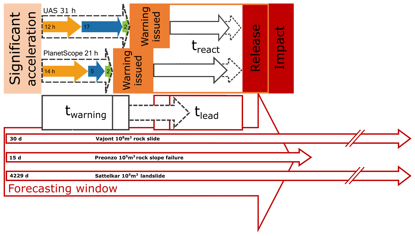
Figure 8Conceptual approach with estimated twarning for the UAS and PlanetScope. Phases of collection, processing and evaluation (indicated as arrows of relative length in orange, blue and green, respectively) (see phases in Figs. 1 and 7) with their total duration time (dashed grey arrows). In twarning, one additional observation requires in sum 31 h for UAS and 21 h for PlanetScope data. Above, major landslides are compared from the onset or displacement detection (solid line) (Petley and Petley, 2006; Anker et al., 2016; Sättele et al., 2016).
Figure 8 is the extension of our concept (see Sect. 1, Fig. 1) systematically supplemented with our estimated time to warning (UAS, PlanetScope) and compared to the few data series pre-dating larger slope failures.
Following a significant acceleration, the forecasting window is opened and twarning starts, which is composed of phases (i) time to collect, (ii) time to process and (iii) time to evaluate. To ascertain a significant acceleration, one further observation is required. Hence, one complete cycle of the three phases, previous analyses and processing iterations are given. Our analysis showed that the UAS and PlanetScope can approach times as short as 31/21 h; as a result tlead is increased, and so is treact.
Assuming both sensors reliably estimate ground motion, solely based on their time requirement, this concept was applied to the temporal development of historic landslide events, thus from measured increased displacements and/or massive accelerations to the final event (Table 7). On this basis we simplified the graph and what we defined as “significant acceleration” using dates of observations such as increased crack opening (Vajont), critical displacement (Preonzo) and the beginning of active ground motion (Sattelkar). Therefore, the opening of twarning and forecasting window are concrete observations of the particular site, independent of any intensity described by the corresponding authors, and allows more freedom for temporal evaluations without going into detail.
For the Preonzo case, the entire 2012 spring period was characterised by high displacement rates. We defined 1 May 2012, when geologists operating the warning system informed local authorities and assembled a crisis team, as the onset or “increased movement” and 15 May 2012 with a rock mass detachment of 300 000 m3 as the impact (Sättele et al., 2016), in total approximately 15 d. For Vajont, the 1 velocity plot by Petley and Petley (2006) (based on data from Semenza and Ghirotti, 2000) shows an increase in movement at about day 60 along with a transition from a linear to an asymptotic trend at approximately day 30, defined as a transition from ductile to brittle. Therefore, we assumed a 30 d forecasting window for twarning and tlead until the impact of the hazardous event on 9 October 1963. However, note that velocities of about 35 mm d−1 are still low and at the minimum of the displacement recognition capability for the digital image correlation method. For the Sattelkar site, the observed mass displacement increase is presumed to have started in 2005 with the 170 000 m3 debris flow event on 31 July 2014 as the impact, thus a window of about 3498 d (Anker et al., 2016).
Even for the Preonzo event, with its short forecasting window of 15 d, the ground motion assessment based on the evaluated optical remote sensing images would have been possible under the assumption of reasonably good UAS flying conditions and the provision of usable PlanetScope images. For twarning there is enough temporal leeway to repeat at least three to four successive measurements comprising the three phases. However, as single accelerations are possible in very short time intervals of less than 2 d, it is impossible to capture these accelerations by means of optical remote sensing methods, given a time requirement of 31 h for the UAS and 21 h for PlanetScope. Nevertheless, this comparison shows that for larger and long-preparing slope failures the technical twarning may well be shorter than the forecasting window starting at the time at which the process becomes predictable. For this type of slope failure, recent developments such as ESA's Geohazards Exploitation Platform (GEP), developed and operated by Terradue, support on-demand services such as the Thematic Exploitation Platforms (TEPs) and have the potential to decrease twarning: the ESA service provides an archive of Copernicus Sentinel-1 and Sentinel-2, Pléiades, and SPOT 6 and SPOT 7 data and access to cloud-computing resources to support large-scale geohazard mapping and monitoring (Volat et al., 2017; Foumelis et al., 2019; Lacroix et al., n.d.). Therefore, the time-critical phases of time to collect and time to process, which in our example are attributed to the larger share of the total time requirement for twarning, could be significantly reduced as the data are directly accessible through high-performance cloud computing. What remains is the third phase, time to evaluate, where a relatively short time is required; thus tlead is extended.
This paper presents an innovative concept to compare the lead time for landslide early warnings of two optical remote sensing systems. We tested this temporal concept by applying UAS and PlanetScope images of temporal proximity as these are currently the sensors with the best spatiotemporal resolution. We assessed the sensors' capability to identify hotspots and to recognise behaviour by delineating ground motion employing digital image correlation (DIC). In so doing, knowing the necessary processing time enabled us to estimate the time requirement and finally to incorporate it into the concept to evaluate sensors with regard to ongoing landslide processes of the Sattelkar as well as historic landslide events.
Our findings derived from DIC for this steep, high alpine case study show that high-resolution UAS data (0.16 m) can be employed to identify and demarcate the main landslide process and reveal its heterogeneous motion behaviour as confirmed by single block tracking. Thus, validated total displacement ranges from 1–4 m and is up to 14 m for 42 d. PlanetScope Ortho Scene data (3 m) can detect the displacement of the landslide central core; however, they cannot accurately represent its extent and internal behaviour. The signal-to-noise ratio, including multiple false-positive displacements, complicates the detection of hotspots at least in this very steep and heterogeneous alpine terrain.
Coarse temporal data resolutions, such as in the case study investigated here, represent an important restriction on the use of optical remote sensing data for landslide early warning applications. Acceleration (and the resulting failure) over short periods of time will likely go unnoticed due to large data acquisition intervals. However, for prolonged acceleration periods, such as observed at the Sattelkar slide and many other relevant hazard sites, the chosen data sources have been demonstrated to represent a formidable early warning approach capable of contributing to an improved risk analysis and evaluation in steep, high alpine regions.
With regard to the temporal aspect for early warning purposes, PlanetScope satellite images require less time compared to the UAS for the time phases of collection, processing and analysing. As a consequence, when time is of the essence, the UAS acquisition cannot compete with the high frequency of PlanetScope daily revisit rates. In general, both are limited in their use as they are passive optical sensors dependent on favourable weather conditions. Nevertheless, with a realistic value of 10 % usable data for our study site, PlanetScope cannot provide daily data as promised.
To conclude, in methodological terms DIC is a reliable tool to derive total displacement of gravitational mass movements even for steep terrain. Given the high reliability of UAS data, its temporal resolution is the key in future attempts to overcome decorrelation due to high ground motions. In addition, a slightly coarser resolution reduces the time needed for total processing and enhances correlation while maintaining spatial accuracy and reliability. PlanetScope is especially interesting as a complementary sensor when UAS employment is restricted, e.g. at inaccessible and/or dangerous sites or for areas too extensive to be covered. For continuous monitoring and early warning, the warning time window could be shortened by on-site drone ports with autonomous acquisition flights and automatic processing. Our systematic evaluation of the sensor capability can be applied to other optical remote sensing sensors, and the same is true for our conceptual approach which extends the lead time. Future studies should focus on the applicability of complementary optical data to confirm the detection of landslide displacement and adjust UAS output resolution as this significantly increases the validity of DIC internal ground motion behaviour.
PlanetScope data are not openly available as Planet Labs, Inc., is a commercial company. However, scientific access schemes to these data exist (https://www.planet.com/, last access: 30 August 2021).
The supplement related to this article is available online at: https://doi.org/10.5194/nhess-21-2753-2021-supplement.
DH developed the study together with MaK and MiK, analysed the data, and wrote the paper. MaK and MiK supported the writing and editing of the paper. IH provided critical proofreading with valuable suggestions. RD is responsible for UAS flight campaigns and processing the images.
The authors declare that they have no conflict of interest.
Publisher’s note: Copernicus Publications remains neutral with regard to jurisdictional claims in published maps and institutional affiliations.
This article is part of the special issue “Remote sensing and Earth observation data in natural hazard and risk studies”. It is not associated with a conference.
This work is supported by a scholarship of the Hanns Seidel Foundation. The authors are grateful to Planet Labs for their CubeSat data via Planet's Education and Research Program. We thank Tobias Koch for the support in fine co-registration of satellite images.
This work was supported by the AlpSenseRely project which is funded by the Bavarian State Ministry of the Environment and Consumer Protection (StMUV).
This paper was edited by Mahdi Motagh and reviewed by Jan Henrik Blöthe and Sigrid Roessner.
Anker, F., Fegerl, L., Hübl, J., Kaitna, R., Neumayer, F., and Keuschnig, M.: Geschiebetransport in Gletscherbächen der Hohen Tauern: Beispiel Obersulzbach, Wildbach- und Lawinenverbauung, 80, 86–96, 2016.
Aubrecht, C., Meier, P., and Taubenböck, H.: Speeding up the clock in remote sensing: identifying the “black spots” in exposure dynamics by capitalizing on the full spectrum of joint high spatial and temporal resolution, Nat. Hazards, 86, 177–182, https://doi.org/10.1007/s11069-015-1857-9, 2017.
Auer, I., Böhm, R., Jurkovic, A., Lipa, W., Orlik, A., Potzmann, R., Schöner, W., Ungersböck, M., Matulla, C., Briffa, K., Jones, P., Efthymiadis, D., Brunetti, M., Nanni, T., Maugeri, M., Mercalli, L., Mestre, O., Moisselin, J.-M., Begert, M., Müller-Westermeier, G., Kveton, V., Bochnicek, O., Stastny, P., Lapin, M., Szalai, S., Szentimrey, T., Cegnar, T., Dolinar, M., Gajic-Capka, M., Zaninovic, K., Majstorovic, Z., and Nieplova, E.: HISTALP – historical instrumental climatological surface time series of the Greater Alpine Region, Int. J. Climatol., 27, 17–46, https://doi.org/10.1002/joc.1377, 2007.
Ayoub, F., Leprince, S., and Keene, L.: User's Guide to COSI-CORR Co-registration of Optically Sensed Images and Correlation, California Institute of Technology, Pasadena, CA 91125, USA, 38 pp., 2009.
Barla, G. and Paronuzzi, P.: The 1963 Vajont Landslide: 50th Anniversary, Rock Mech. Rock Eng., 46, 1267–1270, https://doi.org/10.1007/s00603-013-0483-7, 2013.
Barsi, Á., Kugler, Z., László, I., Szabó, G., and Abdulmutalib, H. M.: ACCURACY DIMENSIONS IN REMOTE SENSING, Int. Arch. Photogramm. Remote Sens. Spatial Inf. Sci., XLII-3, 61–67, https://doi.org/10.5194/isprs-archives-XLII-3-61-2018, 2018.
Batini, C., Blaschke, T., Lang, S., Albrecht, F., Abdulmutalib, H. M., Barsi, Á., Szabó, G., and Kugler, Z.: Data Quality in Remote Sensing, Int. Arch. Photogramm. Remote Sens. Spatial Inf. Sci., XLII-2/W7, 447–453, https://doi.org/10.5194/isprs-archives-XLII-2-W7-447-2017, 2017.
Bickel, V., Manconi, A., and Amann, F.: Quantitative Assessment of Digital Image Correlation Methods to Detect and Monitor Surface Displacements of Large Slope Instabilities, Remote Sens., 10, 1–18, https://doi.org/10.3390/rs10060865, 2018.
Bontemps, N., Lacroix, P., and Doin, M.-P.: Inversion of deformation fields time-series from optical images, and application to the long term kinematics of slow-moving landslides in Peru, Remote Sens. Environ., 210, 144–158, https://doi.org/10.1016/j.rse.2018.02.023, 2018.
Bozzano, F., Mazzanti, P., and Moretto, S.: Discussion to: “Guidelines on the use of inverse velocity method as a tool for setting alarm thresholds and forecasting landslides and structure collapses” by Carlà, T., Intrieri, E., Di Traglia, F., Nolesini, T., Gigli, G., and Casagli, N., Landslides, 15, 1437–1441, https://doi.org/10.1007/s10346-018-0976-2, 2018.
Breger, P.: The Copernicus Full, Free and Open Data Policy, available at: https://www.ecmwf.int/sites/default/files/elibrary/2017/17104-copernicus-full-free-and-open-data-policy_0.pdf (last access: 30 August 2021), 2017.
Butler, D.: Many eyes on Earth, Nature, 505, 143–144, https://doi.org/10.1038/505143a, 2014.
Calvello, M.: Early warning strategies to cope with landslide risk, Rivista Italiana di Geotecnica, 2, 63–91, 2017.
Chae, B.-G., Park, H.-J., Catani, F., Simoni, A., and Berti, M.: Landslide prediction, monitoring and early warning: a concise review of state-of-the-art, Geosci. J., 21, 1033–1070, https://doi.org/10.1007/s12303-017-0034-4, 2017.
Crosetto, M., Monserrat, O., Cuevas-González, M., Devanthéry, N., and Crippa, B.: Persistent Scatterer Interferometry: A review, ISPRS J. Photogramm., 115, 78–89, https://doi.org/10.1016/j.isprsjprs.2015.10.011, 2016.
Crosta, G. B., Agliardi, F., Rivolta, C., Alberti, S., and Dei Cas, L.: Long-term evolution and early warning strategies for complex rockslides by real-time monitoring, Landslides, 14, 1615–1632, https://doi.org/10.1007/s10346-017-0817-8, 2017.
Debella-Gilo, M.: Matching of repeat remote sensing images for precise analysis of mass movements, PhD Thesis, Department of Geosciences Faculty of Mathematics and Natural Sciences, University of Oslo, Oslo, 2011.
Debella-Gilo, M. and Kääb, A.: Sub-pixel precision image matching for measuring surface displacements on mass movements using normalized cross-correlation, Remote Sens. Environ., 115, 130–142, https://doi.org/10.1016/j.rse.2010.08.012, 2011.
Darvishi, M., Schlögel, R., Kofler, C., Cuozzo, G., Rutzinger, M., Zieher, T., Toschi, I., Remondino, F., Mejia-Aguilar, A., Thiebes, B., and Bruzzone, L.: Sentinel-1 and Ground-Based Sensors for Continuous Monitoring of the Corvara Landslide (South Tyrol, Italy), Remote Sens., 10, 1781, https://doi.org/10.3390/rs10111781, 2018.
Delacourt, C., Allemand, P., Berthier, E., Raucoules, D., Casson, B., Grandjean, P., Pambrun, C., and Varel, E.: Remote-sensing techniques for analysing landslide kinematics: a review, B. Soc. Geol. Fr., 178, 89–100, https://doi.org/10.2113/gssgfbull.178.2.89, 2007.
Desrues, M., Lacroix, P., and Brenguier, O.: Satellite Pre-Failure Detection and In Situ Monitoring of the Landslide of the Tunnel du Chambon, French Alps, Geosciences, 9, 1–14, https://doi.org/10.3390/geosciences9070313, 2019.
Dikau, R., Brundsen, D., Schrott, L., and Ibsen, M.-L. (Eds.): Landslide recognition: Identification, Moevement and Courses, Publication/International Association of Geomorphologists, no. 5, John Wiley & Sons, New York, xii, 251, 1996.
Drusch, M., Bello, U. D., Carlier, S., Colin, O., Fernandez, V., Gascon, F., Hoersch, B., Isola, C., Laberinti, P., Martimort, P., Meygret, A., Spoto, F., Sy, O., Marchese, F., and Bargellini, P.: Sentinel-2: ESA's Optical High-Resolution Mission for GMES Operational Services, Remote Sens. Environ., 120, 25–36, https://doi.org/10.1016/j.rse.2011.11.026, 2012.
ESA: eoPortal: Satellite Missions Database, available at: https://directory.eoportal.org/web/eoportal/satellite-missions/, last access: 4 December 2020.
Foumelis, M., Papadopoulou, T., Bally, P., Pacini, F., Provost, F., and Patruno, J.: Monitoring Geohazards Using On-Demand And Systematic Services On Esa's Geohazards Exploitation Platform, in: IGARSS 2019–2019 IEEE International Geoscience and Remote Sensing Symposium, Yokohama, Japan, 28 July–2 August 2019, 5457–5460, 2019.
Froude, M. J. and Petley, D. N.: Global fatal landslide occurrence from 2004 to 2016, Nat. Hazards Earth Syst. Sci., 18, 2161–2181, https://doi.org/10.5194/nhess-18-2161-2018, 2018.
Gariano, S. L. and Guzzetti, F.: Landslides in a changing climate, Earth-Sci. Rev., 162, 227–252, https://doi.org/10.1016/j.earscirev.2016.08.011, 2016.
GeoResearch: Projekt Sattelkar.: Zwischenbericht 1: 2018, NP Hohe Tauern Salzburg, Klimasensitive, hochalpine Kare, Nationalparks Austria, available at: https://www.data.gv.at/katalog/dataset/A5BF75E4-DAEC-5D02-C696-52A478A248AF (last access: 30 August 2021), 2018.
Giordan, D., Hayakawa, Y. S., Nex, F., and Tarolli, P.: Preface: The use of remotely piloted aircraft systems (RPAS) in monitoring applications and management of natural hazards, Nat. Hazards Earth Syst. Sci., 18, 3085–3087, https://doi.org/10.5194/nhess-18-3085-2018, 2018.
Goodchild, M. F.: Scale in GIS: An overview, Geomorphology, 130, 5–9, https://doi.org/10.1016/j.geomorph.2010.10.004, 2011.
Grasso, V. F.: The State of Early Warning Systems, in: Reducing Disaster: Early Warning Systems For Climate Change, edited by: Singh, A. and Zommers, Z., Springer Netherlands, Dordrecht, 109–125, 2014.
Guerriero, L., Di Martire, D., Calcaterra, D., and Francioni, M.: Digital Image Correlation of Google Earth Images for Earth's Surface Displacement Estimation, Remote Sens., 12, https://doi.org/10.3390/rs12213518, 2020.
Hilker, N., Badoux, A., and Hegg, C.: The Swiss flood and landslide damage database 1972–2007, Nat. Hazards Earth Syst. Sci., 9, 913–925, https://doi.org/10.5194/nhess-9-913-2009, 2009.
Huggel, C., Clague, J., and Korup, O.: Is climate change responsible for changing landslide activity in high mountains?, Earth Surf. Proc. Land., 37, 77–91, https://doi.org/10.1002/esp.2223, 2012.
Hungr, O., Leroueil, S., and Picarelli, L.: The Varnes classification of landslide types, an update, Landslides, 11, 167–194, https://doi.org/10.1007/s10346-013-0436-y, 2014.
IPCC (Ed.): Climate change 2014: Synthesis report: Synthesis Report. Contribution of Working Groups I, II and III to the Fifth Assessment Report of the Intergovernmental Panel on Climate Change, Intergovernmental Panel on Climate Change, Geneva, Switzerland, 151 pp., 2014.
Kääb, A., Altena, B., and Mascaro, J.: Coseismic displacements of the 14 November 2016 Mw 7.8 Kaikoura, New Zealand, earthquake using the Planet optical cubesat constellation, Nat. Hazards Earth Syst. Sci., 17, 627–639, https://doi.org/10.5194/nhess-17-627-2017, 2017.
Lacroix, P., Pham, M. Q., and Araujo, G.: MuDsLIdeS: Monitoring and Detection of Landslides from optical Images time-Series, Executive Summary, ESA-Alcantara initiative No 15/P26., n.d.
Lacroix, P., Berthier, E., and Taipe Maquerhua, E.: Earthquake-driven acceleration of slow-moving landslides in the Colca valley, Peru, detected from Pléiades images, Remote Sens. Environ., 165, 148–158, https://doi.org/10.1016/j.rse.2015.05.010, 2015.
Lacroix, P., Bièvre, G., Pathier, E., Kniess, U., and Jongmans, D.: Use of Sentinel-2 images for the detection of precursory motions before landslide failures, Remote Sens. Environ., 215, 507–516, https://doi.org/10.1016/j.rse.2018.03.042, 2018.
Lacroix, P., Araujo, G., Hollingsworth, J., and Taipe, E.: Self-Entrainment Motion of a Slow-Moving Landslide Inferred From Landsat-8 Time Series, J. Geophys. Res.-Earth, 124, 1201–1216, https://doi.org/10.1029/2018JF004920, 2019.
Leprince, S.: Monitoring Earth Surface Dynamics with Optical Imagery, PhD Thesis, California Institute of Technology, https://doi.org/10.7907/ZMTV-GV90, 2008.
Leprince, S., Barbot, S., Ayoub, F., and Avouac, J.-P.: Automatic and Precise Orthorectification, Coregistration, and Subpixel Correlation of Satellite Images, Application to Ground Deformation Measurements, IEEE Trans. Geosci. Remote Sensing, 45, 1529–1558, https://doi.org/10.1109/TGRS.2006.888937, 2007.
Leprince, S., Berthier, E., Ayoub, F., Delacourt, C., and Avouac, J.-P.: Monitoring Earth Surface Dynamics With Optical Imagery, Eos, 89, 1–12, https://doi.org/10.1029/2008EO010001, 2008.
Loew, S., Gschwind, S., Gischig, V., Keller-Signer, A., and Valenti, G.: Monitoring and early warning of the 2012 Preonzo catastrophic rockslope failure, Landslides, 14, 141–154, https://doi.org/10.1007/s10346-016-0701-y, 2017.
Lucieer, A., Jong, S. de, and Turner, D.: Mapping landslide displacements using Structure from Motion (SfM) and image correlation of multi-temporal UAV photography, Prog. Phys. Geog., 38, 97–116, https://doi.org/10.1177/0309133313515293, 2014.
Mazzanti, P., Rocca, A., Bozzano, F., Cossu, R., and Floris, M.: Landslides Forecasting Analysis By Displacement Time Series Derived From Satellite INSAR Data: Preliminary Results, in: FRINGE 2011 Workshop: SP-697, Frascati, Italy, 19–23 September 2011, 2012.
Mazzanti, P., Caporossi, P., and Muzi, R.: Sliding Time Master Digital Image Correlation Analyses of CubeSat Images for landslide Monitoring: The Rattlesnake Hills Landslide (USA), Remote Sens., 12, 592, https://doi.org/10.3390/rs12040592, 2020.
Moretto, S., Bozzano, F., Esposito, C., and Mazzanti, P.: Lesson learned from the pre-collapse time series of displacement of the Preonzo landslide (Switzerland), ROL, 41, 247–250, https://doi.org/10.3301/ROL.2016.140, 2016.
Moretto, S., Bozzano, F., Esposito, C., Mazzanti, P., and Rocca, A.: Assessment of Landslide Pre-Failure Monitoring and Forecasting Using Satellite SAR Interferometry, Geosciences, 7, 1–16, https://doi.org/10.3390/geosciences7020036, 2017.
Noetzli, J., Pellet, C., and Staub, B.: Permafrost in Switzerland 2014/2015 to 2017/2018: Glaciological Report Permafrost No. 16–19 of the Cryospheric Commission of the Swiss Academy of Sciences, Swiss Permafrost Monitoring Network (PERMOS), https://doi.org/10.13093/PERMOS-REP-2019-16-19, 2019.
Pecoraro, G., Calvello, M., and Piciullo, L.: Monitoring strategies for local landslide early warning systems, Landslides, 16, 213–231, https://doi.org/10.1007/s10346-018-1068-z, 2019.
Pesci, A., Giordano, T., Casula, G., Loddo, F., Martino, P. de, Dolce, M., Obrizzo, F., and Pingue, F.: Multitemporal laser scanner-based observation of the Mt. Vesuvius crater: Characterization of overall geometry and recognition of landslide events, ISPRS J. Photogramm., 66, 327–336, https://doi.org/10.1016/j.isprsjprs.2010.12.002, 2011.
Petley, D. N. and Petley, D. J.: On the initiation of large rockslides: perspectives from a new analysis of the Vaiont movement record, in: Landslides from Massive Rock Slope Failure, edited by: Evans, S. G., Scarascia-Mugnozza, G., Strom, A., and Hermanns, R. L., Springer Netherlands, Dordrecht, 77–84, 2006.
Planet Labs: RapidEye Constellation to be Retired in 2020, available at: https://www.planet.com/pulse/rapideye-constellation-to-be-retired-in-2020/, last access: 23 February 2020a.
Planet Labs: Planet Imagery Product Specification: PLANETSCOPE & RAPIDEYE, available at: https://earth.esa.int/eogateway/documents/20142/37627/Planet-combined-imagery-product-specs-2020.pdf, last access: June 2020b.
Plank, S., Krautblatter, M., and Thuro, K.: Feasibility Assessment of Landslide Monitoring by Means of SAR Interferometry: A Case Study in the Ötztal Alps, Austria, in: Engineering Geology for Society and Territory: Volume 2, edited by: Lollino, G., Giordan, D., Crosta, G. B., Corominas, J., Azzam, R., Wasowski, J., and Sciarra, N., Springer International Publishing, Cham, 375–378, https://doi.org/10.1007/978-3-319-09057-3_58, 2015.
Reid, M. E., Baum, R. L., LaHusen, R. G., and Ellis, W. L.: Capturing landslide dynamics and hydrologic triggers using near-real-time monitoring, in: Landslides and engineered slopes: From the past to the future, edited by: Chen, Z., Zhang, J.-M., Ho, K., Wu, F.-Q., and Li, Z.-K., CRC Press, Boca Raton, Florida, 2008.
Rosu, A.-M., Pierrot-Deseilligny, M., Delorme, A., Binet, R., and Klinger, Y.: Measurement of ground displacement from optical satellite image correlation using the free open-source software MicMac, ISPRS J. Photogramm., 100, 48–59, https://doi.org/10.1016/j.isprsjprs.2014.03.002, 2015.
Sättele, M., Krautblatter, M., Bründl, M., and Straub, D.: Forecasting rock slope failure: how reliable and effective are warning systems?, Landslides, 13, 737–750, https://doi.org/10.1007/s10346-015-0605-2, 2016.
Scaioni, M., Longoni, L., Melillo, V., and Papini, M.: Remote Sensing for Landslide Investigations: An Overview of Recent Achievements and Perspectives, Remote Sens., 6, 9600–9652, https://doi.org/10.3390/rs6109600, 2014.
Schrott, L., Otto, J.-C., and Keller, F.: Modelling alpine permafrost distribution in the Hohe Tauern region, Austria, Austrian J. Earth Sc., 105, 169–183, 2012.
Semenza, E. and Ghirotti, M.: History of the 1963 Vaiont slide: The importance of geological factors, B. Eng. Geol. Environ., 59, 87–97, https://doi.org/10.1007/s100640000067, 2000.
Seneviratne, S. I., Nicholls, N., Easterling, D., Goodess, C. M., Kanae, S., Kossin, J., Luo, Y., Marengo, J., McInnes, K., Rahimi, M., Reichstein, M., Sorteberg, A., Vera, C., Zhang, X., Rusticucci, M., Semenov, V., Alexander, L. V., Allen, S., Benito, G., Cavazos, T., Clague, J., Conway, D., Della-Marta, P. M., Gerber, M., Gong, S., Goswami, B. N., Hemer, M., Huggel, C., van den Hurk, B., Kharin, V. V., Kitoh, A., Tank, A. M. K., Li, G., Mason, S., McGuire, W., van Oldenborgh, G. J., Orlowsky, B., Smith, S., Thiaw, W., Velegrakis, A., Yiou, P., Zhang, T., Zhou, T., and Zwiers, F. W.: Changes in Climate Extremes and their Impacts on the Natural Physical Environment, in: Managing the Risks of Extreme Events and Disasters to Advance Climate Change Adaptation: A Special Report of Working Groups I and II of the Intergovernmental Panel on Climate Change, edited by: Field, C. B., Barros, V., Stocker, T. F., and Dahe, Q., Cambridge University Press, Cambridge, 109–230, https://doi.org/10.1017/CBO9781139177245.006, 2012.
Stumpf, A.: Landslide recognition and monitoring with remotely sense data from passive optical sensors, Dissertation, University of Strasbourg, Strasbourg, 2013.
Stumpf, A., Malet, J.-P., Puissant, A., and Travelletti, J.: Monitoring of Earth Surface Motion and Geomorphologic Processes by Optical Image Correlation: Chapter 5, in: Land Surface Remote Sensing: Environment and Risks, edited by: Baghdadi, N. and Zribi, F. M., ISTE Press – Elsevier, 147–190, https://doi.org/10.1016/B978-1-78548-105-5.50005-0, 2016.
Stumpf, A., Michéa, D., and Malet, J.-P.: Improved Co-Registration of Sentinel-2 and Landsat-8 Imagery for Earth Surface Motion Measurements, Remote Sensing, 10, 160, https://doi.org/10.3390/rs10020160, 2018.
Sudmanns, M., Tiede, D., Lang, S., Bergstedt, H., Trost, G., Augustin, H., Baraldi, A., and Blaschke, T.: Big Earth data: disruptive changes in Earth observation data management and analysis?, Int. J. Digit. Earth, 123, 1–19, https://doi.org/10.1080/17538947.2019.1585976, 2019.
TUM: AlpSenseBench: Alpine remote sensing of climate-induced natural hazards, available at: https://www.bgu.tum.de/landslides/alpsensebench/projekt/, last access: 22 September 2020.
Turner, D., Lucieer, A., and Jong, S. de: Time Series Analysis of Landslide Dynamics Using an Unmanned Aerial Vehicle (UAV), Remote Sens., 7, 1736–1757, https://doi.org/10.3390/rs70201736, 2015.
UNISDR: UNISDR Terminology on Disaster Risk Reduction, United Nations Office for Disaster Risk Reduction, Geneva, Switzerland, 2009.
UNISDR: Basics of early warning, Platform for the Promotion of Early Warning, available at: https://www.unisdr.org/2006/ppew/whats-ew/basics-ew.htm (last access: 3 April 2020), 2006.
Volat, M., Lacroix, P., Bontemps, N., and Doin, M.-P.: Introducing “TIO”: Optical imagery time series analysis on the Geohazards Exploitation Platform, in: MDIS ForM@Ter 2017, Besse en Chandesse, 20 October 2017, 2017.
Walter, F., Amann, F., Kos, A., Kenner, R., Phillips, M., Preux, A. de, Huss, M., Tognacca, C., Clinton, J., Diehl, T., and Bonanomi, Y.: Direct observations of a three million cubic meter rock-slope collapse with almost immediate initiation of ensuing debris flows, Geomorphology, 351, 106933, https://doi.org/10.1016/j.geomorph.2019.106933, 2020.
Westoby, M. J., Brasington, J., Glasser, N. F., Hambrey, M. J., and Reynolds, J. M.: “Structure-from-Motion” photogrammetry: A low-cost, effective tool for geoscience applications, Geomorphology, 179, 300–314, https://doi.org/10.1016/j.geomorph.2012.08.021, 2012.