the Creative Commons Attribution 4.0 License.
the Creative Commons Attribution 4.0 License.
 | 25 Aug 2021
Towards an efficient storm surge and inundation forecasting system over the Bengal delta: chasing the Supercyclone Amphan
Md. Jamal Uddin Khan
Fabien Durand
Xavier Bertin
Laurent Testut
Yann Krien
A. K. M. Saiful Islam
Marc Pezerat
Sazzad Hossain
The Bay of Bengal is a well-known breeding ground to some of the deadliest cyclones in history. Despite recent advancements, the complex morphology and hydrodynamics of this large delta and the associated modelling complexity impede accurate storm surge forecasting in this highly vulnerable region. Here we present a proof of concept of a physically consistent and computationally efficient storm surge forecasting system tractable in real time with limited resources. With a state-of-the-art wave-coupled hydrodynamic numerical modelling system, we forecast the recent Supercyclone Amphan in real time. From the available observations, we assessed the quality of our modelling framework. We affirmed the evidence of the key ingredients needed for an efficient, real-time surge and inundation forecast along this active and complex coastal region. This article shows the proof of the maturity of our framework for operational implementation, which can particularly improve the quality of localized forecast for effective decision-making over the Bengal delta shorelines as well as over other similar cyclone-prone regions.
- Article
(2340 KB) - Full-text XML
-
Supplement
(3611 KB) - BibTeX
- EndNote


Storm surges and associated coastal flooding are one of the most dangerous natural hazards along the world coastlines. Annually, storm surges have killed on average over 8000 people and affected 1.5 million people worldwide over the past century (Bouwer and Jonkman, 2018). Among the storm-surge-prone basins, the Bay of Bengal in the northern Indian Ocean is one of the deadliest. This basin has consistently been home to the world's highest surges, experiencing in each decade an average of five surge events exceeding 5 m (Needham et al., 2015). On 18 May 2020, a supercyclone named Amphan was identified as the most powerful ever recorded in the Bay of Bengal, with the highest sustained 3 min wind speed exceeding 240 km/h (130 knots) and the highest 1 min wind gusts reaching 260 km/h (https://www.metoc.navy.mil/jtwc/jtwc.html, last access: 30 May 2020). On 20 May, 2 d later, Amphan made landfall in West Bengal (India), with a sustained wind speed of 112 km/h and gusts of 190 km/h, causing massive damage in India and Bangladesh and claiming at least 116 lives (IFRC, 2020a, b).
The cyclone activity in the Bay of Bengal is very different from the other cyclone-prone oceanic basins (Needham et al., 2015). The basin experiences a distinct bi-modal distribution of cyclonic activity – one with a peak in the pre-monsoon (April–May) and another during post-monsoon (October–November) (Bhardwaj and Singh, 2019). The Bay of Bengal is a small semi-enclosed basin (Fig. 1) which accounts for only 6 % of cyclones worldwide. However, more than 70 % of global casualties from the cyclones and associated storm surges over the last century occurred there (Ali, 1999). The number of fatalities concentrates in the Bengal delta across Bangladesh and India (Ali, 1999; Murty et al., 1986), where more than 150 million people live below 5 m above mean sea level (a.m.s.l.) (Alam and Dominey-Howes, 2014). Seo and Bakkensen (2017) noted a statistically significant correlation between storm surge height and the fatality rate in this region. Two of the notable cyclones that struck this delta include the 1970 Cyclone Bhola and 1991 Cyclone Gorky, which killed about 300 000 (Frank and Husain, 1971) and 150 000 (Khalil, 1993) people, respectively. In recent decades, the death toll has reduced by orders of magnitude. For example, Cyclone Sidr, a Category 5 equivalent cyclone on the Saffir–Simpson scale that made landfall in 2007, claimed 3406 lives (Paul, 2009). At the same time, the cost of material damages has significantly increased (Alam and Dominey-Howes, 2014; Emanuel, 2005; Schmidt et al., 2009). During recent cyclones, government and voluntary agencies of Bangladesh and India made a coordinated effort to evacuate millions of people to safety at cyclone shelters before the cyclone landfall (Paul and Dutt, 2010). This kind of informed coordination benefited from improved communication; increased shelter infrastructure; and, most importantly, from the improvement of the numerical prediction of storm track and intensity.
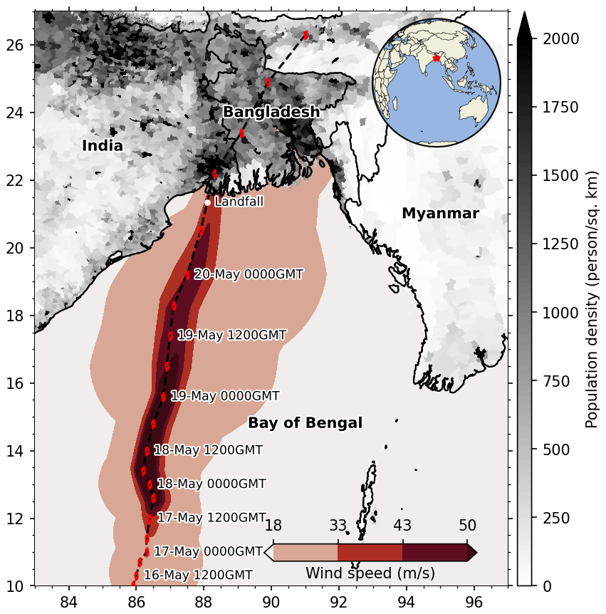
Figure 1The path of the Supercyclone Amphan of May 2020, overlaid on the population density (Center For International Earth Science Information Network (CIESIN), Columbia University, 2016). The footprint of 18 m/s (tropical storm), 33 m/s (Category 1), 43 m/s (Category 2), and 50 m/s (Category 3) wind speed area is shown with the red colour bar (classified as in the Saffir–Simpson scale). Inset shows the location of the study area.
Over the last decades, global weather and forecasting systems have advanced significantly. Several global models now run multiple times a day, starting from multiple initial conditions, with horizontal resolutions on the order of tens of kilometres, providing forecasts with a range of hours to a week. These forecasts have proven useful during weather extremes like tropical storms (Magnusson et al., 2019). Operational hurricane forecasting systems like Hurricane Weather Research and Forecasting (HWRF) have emerged and reached a level of maturity to provide reliable cyclone forecasts several days in advance throughout the tropics (Tallapragada et al., 2014).
Storm surge forecasting has been developed and implemented around the world along with the advancement of the weather and storm forecasting (Bernier and Thompson, 2015; Daniel et al., 2009; Flowerdew et al., 2012; Lane et al., 2009; Verlaan et al., 2005). Nowadays, operational surge forecasting systems typically run on high-performance computing systems, either on a scheduled basis or triggered on-demand during an event (Loftis et al., 2019; Oliveira et al., 2020; Khalid and Ferreira, 2020). In the Bay of Bengal region, the Indian Institute of Technology-Delhi (IIT-D) storm surge model has been running operationally with a horizontal resolution of 3.7 km for 1 decade (Dube et al., 2009). Under the Tropical Cyclone Program (TCP) of the World Meteorological Organization (WMO), the IIT-D model is also implemented to run in the Bangladesh Meteorological Department (BMD). Beside the IIT-D model, the BMD also experimentally uses the Meteorological Research Institute (MRI) storm surge model from the Japan Meteorological Agency (JMA) (http://bmd.gov.bd/p/Storm-Surge, last access: 30 May 2020). Storm surge forecasts have shown their potential to better target the evacuation decision, to optimize early-engineering preparations, and to improve the efficiency of the allocation of the resources (Glahn et al., 2009; Lazo and Waldman, 2011; Munroe et al., 2018). Availability of a spatially distributed forecast of storm surge flooding can further increase the fluidity of communication toward the public (Lazo et al., 2015). Keeping in mind the cyclonic surge hazards over the densely populated Bengal delta, having a reliable real-time operational forecast system in the region would be extremely valuable and would address a societal demand (Ahsan et al., 2020). The major challenges in operating and maintaining such systems are manifold for the Bengal delta, including lack of expertise, limitations of funding resources to operate and maintain necessary infrastructure and datasets, and availability of reliable modelling systems in operational mode (Roy et al., 2015).
Storm surge modelling is, however, computationally expensive and has proven to be challenging in real-time-forecasting mode (Glahn et al., 2009; Murty et al., 2017). Several practical solutions exist to curb the real-time constraints of cyclone forecasts, such as soft real-time computation based on looking up an extensive database of pre-computed cyclones (Condon et al., 2013; Yang et al., 2020), coarse-resolution modelling (Suh et al., 2015), and modelling without wave-coupling (Murty et al., 2017). Over the past decades, unstructured-grid modelling systems are getting more and more popular due to their efficiency in resolving the topographic features and their reduced computational cost compared to structured-grid equivalents (Ji et al., 2009; Lane et al., 2009; Melton et al., 2009; Fortunato et al., 2017; Khalid and Ferreira, 2020).
The published history of storm surge modelling in the northern Bay of Bengal goes hand in hand with the land-falling of very severe cyclones (Das, 1972; Flather, 1994; Dube et al., 2004; Murty et al., 2014; Krien et al., 2017). From the modelling of the historical storm events, previous studies have identified several ingredients as essential for accurate modelling and forecasting of storm-surge-induced water level and associated flooding over the Bengal delta. The most important of these ingredients is an accurate bathymetry and topography (Krien et al., 2016, 2017; Murty et al., 1986). Second, it is required to have a large-scale modelling domain comprising the whole Ganges–Brahmaputra–Meghna (GBM) estuarine network (Johns and Ali, 1980; Oliveira et al., 2020) at a high-enough model resolution (Krien et al., 2017; Kuroda et al., 2010). The modelling framework is required to simulate tide and surge together to account for the tide–surge interactions (As-Salek and Yasuda, 2001; Johns and Ali, 1980; Kuroda et al., 2010; Murty et al., 1986). Furthermore, an online coupling of the hydrodynamics and the short waves is also necessary to account for the wave set-up (Deb and Ferreira, 2016; Krien et al., 2017). The capability of the model to simulate the wetting and drying is also necessary to model the inundation (Madsen and Jakobsen, 2004).
Fully coupled tide–surge–wave models have been recommended for operational forecasting in the Bay of Bengal for years (Johns and Ali, 1980; Murty et al., 1986; As-Salek and Yasuda, 2001; Deb and Ferreira, 2016; Krien et al., 2017). Besides the development of the wave–ocean coupled hydrodynamic modelling tool itself, the main challenge in implementing such a system is due to the high computational requirements for the modelling systems (Murty et al., 2014, 2016). Due to these constraints, operational systems are commonly run with either only a surge or coupled tide–surge model at kilometric resolution (Dube et al., 2009). In recent years, higher resolution (100 m at the coast) unstructured-grid models have been used for operational forecasts over part of Indian coastlines in the Bay of Bengal but without wave-coupling (Murty et al., 2017). These limitations in operational forecasting systems can significantly impede a proper interpretation during an actual cyclonic storm, as discussed in the next section through a set of hindcast sensitivity experiments of Cyclone Amphan.
Cyclone Amphan is not only the latest event on record in the Bay of Bengal but also the costliest event that struck this shoreline, with an estimated bill of over USD 14 billion in West Bengal and Bangladesh (DhakaTribune, 2020; IFRC, 2020a). During this cyclone, we have proactively forecast storm surge in real time with common computational resources using a high-resolution coupled modelling system forced by a combination of freely available atmospheric forecasts. The general goal of this paper is to provide a proof of concept of a tractable operational storm surge forecasting system over this key region of vulnerability, to identify the key ingredients of such a system, and to provide guidance in the near-future initiatives of the operational forecasting community. First, we present the various processes governing the surge dynamics to illustrate the challenges of modelling storm surges in the Bay of Bengal in Sect. 2. Section 3 documents the atmospheric forecasts that are required to generate a surge forecast. In Sect. 4, we introduce our numerically efficient hydrodynamics–waves coupled modelling platform and present its practical real-time computational set-up in Sect. 5. Finally, we present the remaining modelling and forecasting issues in Sect. 6. Section 7 provides a conclusion to this study.
The Bay of Bengal is a macro-tidal region where peak tidal range reaches as high as 5 m over the north-eastern corner of the bay (Krien et al., 2016; Tazkia et al., 2017). A large geographical extent of the land–sea hydraulic continuum with an intricate estuarine network complicates the water level dynamics in this part of the coastal ocean. During a cyclone, the dynamics get even more complicated due to wave-induced set-up and tide–surge interaction. In Fig. 2, we illustrate a simplified view of water level components – tide, surge, wave set-up – and their interactions with the topography in driving inundation during a cyclone.
During a cyclone, the atmospheric pressure drop and the wind stress both generate the water level surge. This atmospheric storm surge is non-linearly dependent on the astronomical tide. The dependent nature of both tide and surge implies that the surge induced by a given meteorological condition differs at different stages of the tide, particularly in the nearshore shallow zone. This departure from linearly added tide and surge component is known as tide–surge interaction. In a macro-tidal region like the Bengal delta, tide–surge interaction typically amounts to several tens of centimetres (Antony and Unnikrishnan, 2013; Idier et al., 2019). Due to this interaction, the highest surge (water level – tide) does not coincide with high tide as shown from observations (Antony and Unnikrishnan, 2013) and numerical modelling (Krien et al., 2017; Antony et al., 2020). The strong dependence on tide reinforces the importance of having an accurate tidal model for the region and a reliable network of water level gauge for validation (As-Salek and Yasuda, 2001; Krien et al., 2017; Kumar et al., 2015; Murty et al., 2016).

Figure 2Conceptual diagram of the involved processes that determine the water level evolution and its interaction with the controls determining the inland flooding.
Wave set-up is another component that has a significant impact on the nearshore sea level (Idier et al., 2019; Krien et al., 2017; Murty et al., 2014). It manifests as an increase in the sea level occurring in the nearshore zone that accompanies the dissipation of short waves by breaking (Longuet-Higgins and Stewart, 1962). During Cyclone Sidr, the modelled wave set-up was around 30 cm (Krien et al., 2017). This estimation would be potentially underestimated by up to 100 % due to an early dissipation of wave energy by depth-induced breaking arising from usual parameterizations utilized in spectral wave models (Pezerat et al., 2020, 2021).
At the seasonal scale, the mean sea level around the Bengal delta also shows considerable evolution. The amplitude of this variation can go as high as 40 cm due to freshwater influxes during the monsoon from the GBM river system and offshore-ocean steric variability (Durand et al., 2019; Tazkia et al., 2017). During the wintertime cyclone-prone season, this steric variability can induce 10–15 cm variation in mean sea level of the bay.
Except for the Sundarban mangrove forest, coastal Bangladesh is mostly embanked through a network of 139 polders (Nowreen et al., 2013). These embanked areas can be flooded in three ways: (a) by overflowing or overtopping, (b) by breaching of the embankments or control structures, and (c) by heavy rainfall inside the embanked area. The height of these embankments plays the most vital role in actuating the inundation from a storm surge (Krien et al., 2017). The performance of the embankments during the cyclone is another crucial factor, depending on the composition (typically, earth vs. stones or concrete). During a cyclone, the wave action as well as overtopping and overflowing on the embankments can create breaches at a weak point, thus creating local inland flooding (Islam et al., 2011). Particularly for Bangladesh, the consequence of such storm-surge-induced flooding can be long-lasting as the topography inside polders is often below the mean sea level due to ground compaction (Auerbach et al., 2015).
On 13 May 2020, a low-pressure area was persisting over the northern Bay of Bengal about 300 km east of Sri Lanka. By the end of 15 May, the Joint Typhoon Warning Center (JTWC) upgraded the low-pressure system to a tropical depression. The Indian Meteorological Department (IMD) also reported the same development on the next day. The tropical depression continued to move northward and intensified into the cyclonic storm Amphan by 16 May 18:00 UTC. During the following 12 h, the intensification of the system was limited. However, starting from 12:00 UTC on 17 May, Amphan started to intensify very rapidly. In just 6 h, around 18:00 UTC, the maximum wind speed increased from 140 to 215 km/h, making it an extremely severe cyclonic storm (equivalent to Category 4 on the Saffir–Simpson scale). Over the next 12 h, Amphan continued to intensify, reaching a maximum of 260 km/h wind speed and 907 mbar central pressure, making it the most intense event on record in the Bay of Bengal. During this time, it appeared to form two distinct eye walls, which is typical of intense cyclones. Over the next 24 h, Amphan lost most of its strength due to the eye wall replacement cycle in the presence of moderate vertical wind shear (30–40 km/h). The system continued to decay due to easterly shear and mid-level dry air. The vertical wind shear remained moderate during this period. The cyclone made landfall between 08:00 and 10:00 UTC around 88.35∘ N, 21.65∘ E (Fig. 1), at mid-tide. At landfall, the reported central pressure amounted to 965 mbar, with a maximum wind speed of 150–160 km/h. Afterwards, over its journey inland, the system further eroded and disappeared by 21 May. The black lines in Fig. 3 illustrate the evolution of Amphan from the JTWC best track.
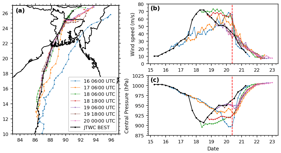
Figure 3Temporal evolution of the successive forecasts of Amphan cyclone wind and pressure. (a) Forecast track colour-coded with the date (JTWC best track in black). (b) Wind speed forecast with each epoch. (c) Pressure forecast with each epoch. The vertical dashed red line indicates the time of landfall.
The extended range outlook by the IMD published on 7 May predicted cyclogenesis to occur between 8 and 14 May with low probability (IMD, 2021). Global and regional models started to predict that a significant storm would happen in the Bay of Bengal as early as 12 May, 8 d before the cyclone landfall and 4 d before the actual formation of the tropical depression. The formation of the low-pressure system triggered the operational HWRF system of the NOAA (https://www.emc.ncep.noaa.gov/gc_wmb/vxt/HWRF/, last access: 30 May 2020) on 14 May. Similarly, the operational system of the IMD (https://nwp.imd.gov.in/hwrf/IMDHWRFv3.6) was also triggered a day later. For the rest of the paper, we confine our analysis to the forecast disseminated by the NOAA-HWRF only, relying on the Automated Tropical Cyclone Forecasting System (ATCF) text output (Miller et al., 1990). Figure 3 illustrates a few of the selected forecast cyclone tracks sequentially issued from the NOAA-HWRF.
The forecasts illustrate the convergence of the location of the landfall. As early as 17 May, 3 d before the landfall, the forecast tracks had converged towards the observed track. On 18 May, 1 d later, the forecast error in the storm track location had reduced to around 50 km. The forecast wind speed and central pressure did not show as much accuracy as the forecast trajectory. The initial forecasts captured the magnitude of the intensification. However, they failed to forecast the rapid intensification that occurred during 17–18 May. On the other hand, the subsequent forecasts initiated during 17 and 18 May failed to capture the rapid weakening of the system that occurred over 19–20 May, before landfall. Overall, in terms of wind speed, the forecast evolution was accurate (within 5 m/s) only at a 24 h range.
We have developed our tide and storm surge model based on the community and open-source modelling platform SCHISM (Semi-implicit Cross-scale Hydroscience Integrated System Model) developed by Zhang et al. (2016b) – a derivative code of the SELFE (Semi-implicit Eulerian–Lagrangian Finite Element) model, originally developed by Zhang and Baptista (2008). This model solves the shallow-water equations using finite-element and finite-volume schemes in an unstructured grid that can combine tri- and quad-elements. The model is applicable in baroclinic as well as barotropic ocean circulation problems for a broad range of spatial scales, from the creek scale to the ocean basins (Ye et al., 2020; Zhang et al., 2020, 2016a). It has already been shown to have an excellent performance in reproducing shallow-water processes over the Bengal shoreline and elsewhere, including the coastal tide (Krien et al., 2016), wave set-up (Guérin et al., 2018), and storm surge flooding (Bertin et al., 2014; Krien et al., 2017; Fernández-Montblanc et al., 2019).
4.1 Model implementation
We have implemented our model on an updated bathymetry of Krien et al. (2016) with the additional inclusion of 77 000 digitized sounding points from a set of 34 nautical charts published by the Bangladesh Navy (Khan et al., 2019) (See Supplement Fig. S1). Our bathymetric dataset is a combination of two digitized sounding datasets in the nearshore zone – one from navigational charts produced by the Bangladesh Navy and another being a bathymetry of the Hooghly estuary provided by the IWAI (Inland Waterways Authority of India). Depending on the sounding points, these observations are 7 to 20 years old. The river bathymetry is composed of a set of cross-sections obtained from the Bangladesh Water Development Board (BWDB), which is further interpolated at about 300 m resolution using a dedicated 1D river modelling tool and GIS techniques. The south-central part of the delta is composed of a high-resolution (50 m) inland topography (see Supplement Fig. S2). We considered the General Bathymetric Chart of the Oceans (GEBCO) 2014 bathymetry to complement in the deeper part of the ocean (https://www.gebco.net/data_and_products/gridded_bathymetry_data/, last access: 20 June 2020) and the Shuttle Radar Topography Mission (SRTM) digital elevation model for the rest of the inland topography as appearing in the GEBCO 2014 dataset (https://www2.jpl.nasa.gov/srtm/cbanddataproducts.html, last access: 20 June 2020). Our unstructured model mesh was developed based on this blended bathymetry, covering the northern Bay of Bengal (11 to 24∘ N) with a variable resolution based on the shallow-water wave propagation and bottom slope criteria. Our model grid consists of about 600 000 nodes and 1 million elements in total. The resulting grid resolution ranges from 250 m in the estuaries and the delta to 15 km in the deeper part of the central Bay of Bengal. The model domain and mesh are identical to those presented in Khan et al. (2019) (Fig. 4).
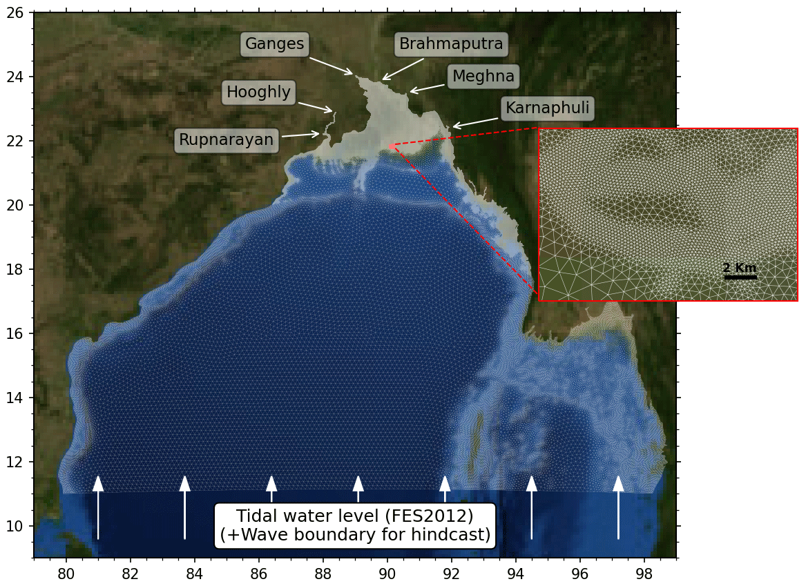
Figure 4Computational domains and model mesh for SCHISM–WWMIII as well as model boundary conditions. White arrows on the southern boundary show the forcing with the tidal solution provided by FES2012, and on the northern boundary they show the river discharges. For a hindcast experiment, wave spectra from WW3 are imposed on the southern boundary. The background is taken from Blue Marble: Next Generation, credited to NASA Earth Observatory.
To account for the effect of short waves on the mean circulation, the Wind Wave Model III (WWMIII), a third-generation spectral wave model, is coupled at source code level with SCHISM in our modelling framework (Roland et al., 2012). In our configuration, the WWMIII solves the wave action equation on the native SCHISM grid using a fully implicit scheme. The source terms in our model comprise the energy input due to wind (Ardhuin et al., 2010), the non-linear interaction in deep and shallow water, energy dissipation in deep and shallow water due to white capping and wave breaking, and energy dissipation due to bottom friction. We run the WWMIII with 12 directional and 12 frequency bins. Every 30 min of SCHISM runtime, water level and currents are passed to the WWM for calculating the evolution of the wave fields. Calculated wave radiation stress, total surface stress, and the wave orbital velocity are passed back to SCHISM before computing the next time step. Wave breaking is modelled according to Battjes and Janssen (1978). As the nearshore region of the Bengal delta has a very mild slope, the value for the breaking coefficient α, which controls the rate of dissipation, was reduced from 1 to 0.1 to avoid over-dissipation (Pezerat et al., 2020, 2021). The WWMIII was also forced along the model's southern open boundary by time series of directional spectra, computed from a large-scale application of the WaveWatch3 (hereafter WW3) model (WW3DG, 2019). The WW3 was implemented at the scale of the whole Indian Ocean with a spatial resolution of 0.5∘ and forced by the final analysis (FNL) reanalysis wind data at a 3 h time step (National Centers for Environmental Prediction, National Weather Service, NOAA, U.S. Department of Commerce, 2015).
4.2 Model forcings
Our model is forced over the whole domain by the astronomical tidal potential for the 12 main constituents (2N2, K1, K2, M2, Mu2, N2, Nu2, O1, P1, Q1, S2, T2). At the southern boundary, we have prescribed a boundary tidal water level from 26 harmonic constituents (M2, M3, M4, M6, M8, Mf, Mm, MN4, MS4, Msf, Mu2, N2, Nu2, O1, P1, Q1, R2, S1, S2, S4, Ssa, T2, K2, K1, J1, and 2N2) extracted from the FES2012 global tide model (Carrère et al., 2013). At open upstream-river boundaries of the Ganges and Brahmaputra, a discharge time series from the BWDB is forced for the benchmark tidal simulation, and a climatologic discharge time series is applied for storm surge simulations during Amphan. A discharge climatology is applied at Hooghly (Mukhopadhyay et al., 2006) and Karnaphuli (Chowdhury and Al Rahim, 2012). At Meghna and Rupnarayan open river boundaries, we implemented a radiating Flather boundary condition. From a year-long tidal simulation, we found that the updated version of the bathymetry performs 2–4 times better at key locations compared to the global tidal models, which include Finite Element Solution (FES; Carrère et al., 2013), Goddard Ocean Tide (GOT; Ray, 1999), and TOPEX/POSEIDON (TPXO; Egbert and Erofeeva, 2002) (see Supplement Table S1).
We derived the atmospheric wind and pressure fields for SCHISM from a blending of analytical wind field inferred from a parametric wind model (close to the cyclone track) and background atmospheric field from the Global Forecast System (GFS; https://www.ncdc.noaa.gov/data-access/model-data/model-datasets/global-forcast-system-gfs, last access: 30 May 2020) reanalysis (farther away) following Krien et al. (2017, 2018). We used the best-track data of the JTWC provided at a 6 h time step as input for the analytical wind and pressure field. Here we choose the analytical wind profile of Emanuel and Rotunno (2011) and the analytical pressure field profile of Holland (1980). To be consistent with our forecast described in Sect. 5, the background wind field was generated incrementally from an accumulative merging of GFS forecasts for each 6 h forecast window, with a 1 h time step. The analytical and background wind fields were first temporally interpolated every 15 min and overlaid on the background GFS fields using a distance-varying weighting coefficient for the cyclone centre to ensure a smooth transition (Fig. 7b). We took into account the asymmetry of the cyclonic wind field following Lin and Chavas (2012). The final resolution after merging the analytical wind field with the interpolated background GFS fields is 0.025∘. For all storm surge simulations, a spinup time of 2 d is considered in this study.
4.3 Predictive skills
With the above-described model set-up, we ran our model to calculate the water level and sea state evolution during Amphan. The simulation was done a posteriori once the cyclone had passed and with JTWC and GFS hindcasts being already available throughout the cyclone lifetime. Figure 5 shows comparisons between observed and modelled significant wave height (SWH), peak wave period, and water level. First, we compare the significant wave height derived from the altimetric estimate of Sentinel-3B processed by the Wave Thematic Assembly Center from the Copernicus Marine Environment Monitoring Service (https://scihub.copernicus.eu/, last access: 18 June 2020), which overpassed on 18 May 2020 at 16:03 GMT. For each altimetric data point inside our domain, we interpolated the model output using a nearest-neighbour approach, both spatially and temporally. This comparison shows that SWH is reasonably reproduced, with RMSE typically within 1 m (within 18 % of the mean value). However, we observed an overestimation of SWH of about 2.5 m near the cyclone centre. One of the reasons for such a difference is a limitation of analytical wind field models, as discussed by Krien et al. (2017).
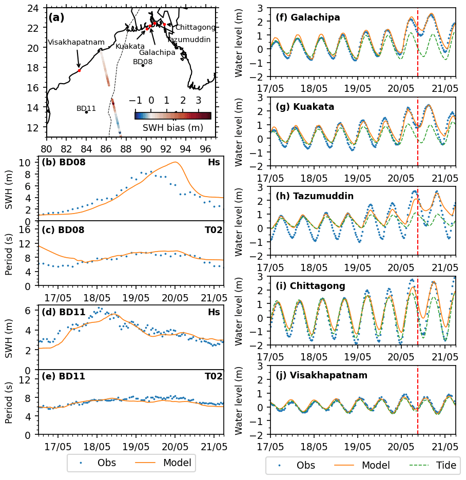
Figure 5Comparison of simulated (in orange) and observed (in blue) water level, significant wave height (SWH), and mean wave period. (a) The map shows the along-track bias in SWH compared to the one calculated from Sentinel-3B altimeter overpass at 18 May 2020 16:03 Z. The bottom panel shows the modelled SWH and mean wave period (orange line) compared to buoy observations (blue dots) at BD08 (b–c) and BD11 (d–e) provided by INCOIS. Comparison between observed (blue dots) and modelled (orange line) water level at the station locations – (f) Galachipa, (g) Kuakata, (h) Tazumuddin, (i) Chittagong, and (j) Visakhapatnam. Green dashed lines in (f)–(k) indicate the modelled tidal water level. Locations of the buoys and the water level gauges are shown in (a). The vertical red lines in water level plots indicate the time of landfall.
We present an in-situ-observed time series of SWH and mean wave period during the life cycle of Amphan in Fig. 5 for BD08 (Fig. 5b–c) and BD11 (Fig. 5d–e) oceanographic buoys (the dataset is collected from the Indian National Centre for Ocean Information Services (INCOIS) data portal at https://incois.gov.in/portal/datainfo/mb.jsp, last access: 30 May 2020). The two buoys are located on either side of the Amphan track, 250 km to its east and 230 km to its west, respectively. We can see that at both locations, the model reproduces the SWH well. The match is particularly good at BD11, consistently within 1 m of the observed evolution. At BD08, SWH is found to be overestimated by about 2 m at its peak, with a 12 h lead shift in time. Such a difference can come from positional and timing uncertainties in JTWC best-track data, from our assumption of a constant translational velocity in between each 6-hourly JTWC time step, and finally from the intrinsic uncertainty in the analytical wind field itself, as shown in Fig. 3b. Despite multiple sources of potential errors and uncertainties, our model appears capable of capturing the general features of the sea state, both significant wave height (SWH) and period, relatively well. The overall predictive skills of the model in terms of short waves are only slightly below those from hindcast exercises typically conducted over other ocean basins using similar modelling strategies (Bertin et al., 2014; Krien et al., 2018).
The real-time availability of observed water level time series in this region is relatively scanty. We were able to access only a handful of coastal water level records, most of them located eastward of the landfall location. The right panels of Fig. 5f–j illustrated the comparison of the recorded water level and modelled storm surge. Among these tide gauges, Chittagong (Fig. 5i) and Visakhapatnam (Fig. 5j) time series are retrieved from the UNESCO Intergovernmental Oceanographic Commission (IOC) sea level monitoring service (http://www.ioc-sealevelmonitoring.org/map.php, last access: 18 June 2020), and the rest are provided by the Bangladesh Inland Water Transport Authority (BIWTA; http://www.biwta.gov.bd/, last access: 18 June 2020). The datum for water level time series at Chittagong and Visakhapatnam is changed from in situ datum to MSL by removing long-term mean. The time series provided by the BIWTA are already referenced to MSL and thus kept unchanged. We also plotted the reconstructed tidal water level from the tidal atlas derived from our model. The overall tidal propagation is well simulated in Galachipa and Kuakata, while at Tazumuddin the simulation tidal range is found to be underestimated. The local bathymetric error and friction parameterization might be the source of the discrepancy. Tide gauge at Tazumuddin is situated at the mouth of the Meghna, where bathymetry is rapidly changing (Khan et al., 2019). However, our model correctly reproduces the peak of the water level at all locations. The maximum recorded water level at these stations is around 2–2.5 m a.m.s.l., with a storm surge (water level – tide) of the same order of magnitude.
To spatially assess the storm surge generated by Cyclone Amphan, we first take a look into the temporal maximum water level in Fig. 6a. We can see that the whole coastal region experienced a high water level ranging from 2–5 m for Amphan. To quantify the contribution of the cyclone, we have looked in the surge component, defined as the difference between the total modelled water level and a tide-only simulation. Figure 6b illustrates the temporal maximum of surge over the delta region. The highest surge level is 5 m around the location of the landfall (21.6∘ N, 88.3∘ E). The maximum non-linear interaction between tide and surge amounts to about 30 cm in the nearshore domain (Fig. 6d).
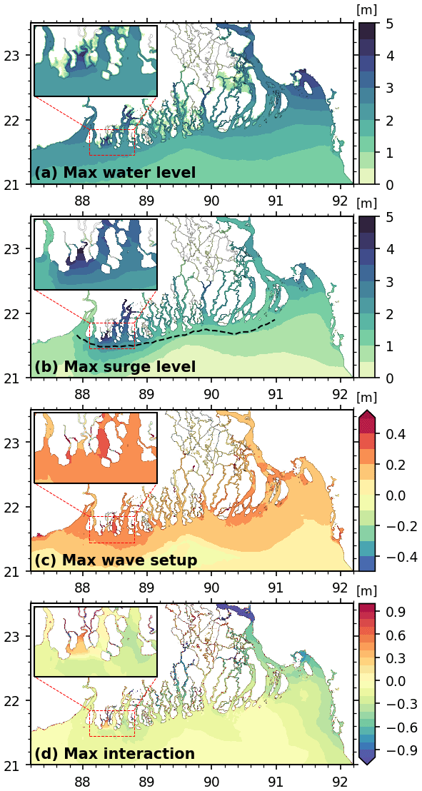
Figure 6Hindcast of (a) maximum water level, (b) maximum surge, wave set-up and set-down, and (d) maximum non-linear interaction between tide and surge. For (a), for the areas above mean sea level, the water level is converted to water level above the topography for consistency. The inset maps show a close-up (75 km × 45 km) of the landfall region. The dashed black line shown in (b) is the segment for error analysis of the forecast experiment in Sect. 5.
To quantify the contribution of the wave set-up, we re-calculated the storm surge without the coupling with the wave model. Figure 6c shows the maximum of the difference between the two simulated water levels. In general, wave set-up contributes to the Amphan storm surge by about 20 cm all along the Bengal shoreline and locally over 30 cm close to the cyclone landfall. Nevertheless, the spatial resolution at the nearshore region employed in this study (250 m) is still too coarse for capturing the maximum wave set-up that develops along the shoreline, where a resolution of a few tens of metres should be employed (Guérin et al., 2018). Nonetheless, this comparison shows that wave set-up not only is developed along the shoreline exposed to waves but affects the whole delta up to far upstream, a process already observed over large estuaries (Bertin et al., 2015; Fortunato et al., 2017).
Table 1Data sources for the model forcings.

n/a: not applicable. * Last access: 30 May 2020.
Our findings reaffirm the necessity of a proper coupling between tide, surge, and wave to forecast the water level evolution. For Amphan, the magnitude of tide–surge interaction amounts to about 10 % of the maximum total water level with spatial variation. Similarly, the magnitude of wave set-up is also spatially varying, with a typical amplitude of 10 %–15 % of the maximum total water level. This non-negligible, non-linear dependency shows the importance of a fully coupled hydrodynamics–wave modelling system for a successful forecast of the water levels in the hydrodynamic setting of the Bengal delta. Our modelling framework showed reasonable accuracy in reproducing observed storm surge water level along the Bengal coastline. The accuracy is in line with the typical level of performance of similar systems applied elsewhere in the world ocean (Bertin et al., 2015; Fernández-Montblanc et al., 2019; Suh et al., 2015). The hindcast experiment thus shows the viability of our model for a proof of concept of a real-time forecasting exercise.
The current state of maturity of atmospheric real-time cyclone forecast products allows their application to real-time surge forecasting, as discussed in Sect. 3. As explained in Sect. 2, the storm surge generated from cyclones depends on the atmospheric pressure, wind, and background (typically tidal) water level. In this section, a near-real-time storm surge forecasting scheme is presented using a publicly available atmospheric forcing dataset.
5.1 Forecast strategy and forcing products
During Cyclone Amphan, we performed near-real-time storm surge forecasts based on our model. In our forecasts, we relied on the outputs of global models (GFS and HWRF) and advisories (JTWC) for the estimates of the atmospheric forcing. These advisories and global models are updated every 6 h. Similar to the GFS forecast cycle, we updated our forecasts at every 00:00, 06:00, 12:00, and 18:00 UTC.
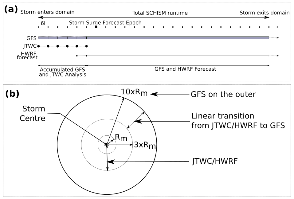
Figure 7(a) Temporal combination scheme of the JTWC, GFS, and HWRF forecasts for each 6-hourly storm surge forecast epoch. (b) Spatial blending of the analytical and GFS wind and pressure field.
For each forecast, we derived the atmospheric forcing from a blend of JTWC, HWRF, and GFS data (Table 1). The JTWC publishes storm advisories at 03:00, 09:00, 15:00, and 21:00 UTC. The advisory includes an analysis of the storm intensity and position from a satellite fix 3 h prior, followed by a forecast for the following 72 h, with 6 to 12 h time steps. The NOAA published their HWRF model advisory for each GFS forecast cycle at 3 h time steps. The GFS provides the wind and pressure fields in hourly time steps at a 0.25∘ regular spatial grid. The GFS model is initialized 6-hourly at 00:00, 06:00, 12:00, and 18:00 UTC, and the data are available 3 h after the initialized period.
The wind and pressure fields around the centre of the storm are derived analytically from a concatenated JTWC and HWRF. We used GFS data as the background wind and pressure on the outer region of the analytical fields.
We initiated our forecast cycles on 16 March 2020 at 06:00 UTC, utilizing the first advisory from the JTWC published at 03:00 UTC merged with the forecast from the HWRF issued at 18:00 UTC of the preceding day. We took the background wind and pressure field from the GFS forecast published at 00:00 UTC. In the subsequent forecast cycles, we updated the previous track file by first replacing the past time steps with the analysis from the latest JTWC advisory, then appending the forecasts from the HWRF again. For the background wind and pressure fields from the GFS, we retained the first 6 h of forecasts from the previous cycles and updated the remainder of the time series from the latest forecast with new initialization. For each forecast cycle, we kept the starting time of our model the same, on 16 May at 00:00 UTC, and ran it until 1 d after the landfall for a consistent initial condition. This approach is feasible as the storms in the Bay of Bengal typically form, grow, and dissipate in about a week. A graphical representation of our strategy to temporally concatenate JTWC, GFS, and HWRF forecasts over a forecast cycle is shown in Fig. 7a. The spatial blending of the analytical and GFS wind and pressure field is illustrated in Fig. 7b.
5.2 Real-time computation and results
Since our forecast is contingent on the JTWC advisory of 3 h before, we only had a 3-hour-long window to achieve the pre-processing of the forcing files, to run the model, and to complete the necessary post-processing of the model outputs. The numerical efficiency of our model made it possible to cope with this time constraint of the forecast, using a modest computing resource. The computing environment we used is detailed in Table 2, which essentially amounts to a single desktop computer fitted with a high-end consumer-grade processor.
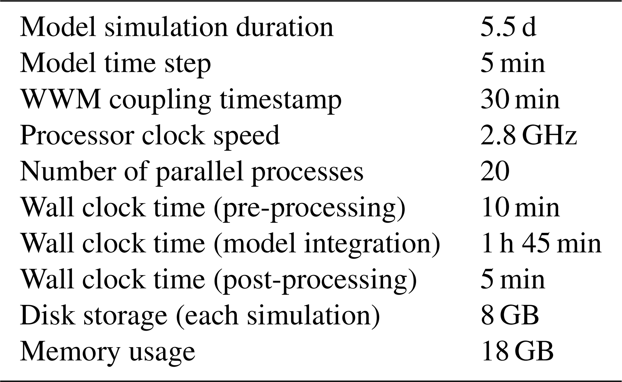
Figure 8 illustrates the evolution of the maximum total water level and surge for the corresponding forecasts issued at T−60 h, T−36 h, and T−12 h, where T is the time of landfall (20 May 2020 at 08:00 to 10:00 UTC). For the forecast issued at T−60 h, the cyclone landfall is located near 90∘ E, associated with the strong surge simulated over the surrounding area. As the atmospheric cyclone forecasts gradually converge towards the actual landfall location more than 100 km westward, so do our storm surge forecasts at T−36 h and T−12 h. The dependency of the timing of the landfall on the forecast range is notable here. At T−36 h, the maximum water level pattern is similar to the hindcast shown in Fig. 6. By T−12 h, the magnitude of the forecast maximum water level corresponds well with the hindcast estimate.
To substantiate the gradual increase in the quality of the forecasts, we compared the maximum surge level predicted at the various forecast ranges (T−60 h, T−36 h, T−12 h) with the hindcast experiment along a line encompassing the nearshore delta (segment displayed in Fig. 6). The results show that, in the T−60 h forecast, the location of maximum surge appears offset eastward by as much as 150 km. The magnitude of the maximum surge is also poorly predicted, with an overestimation of about 3 m. In the T−36 h forecast, the location of the maximum surge appears largely corrected, but the magnitude of the peak remains overestimated by about 3 m. In the T−12 h forecast, both the location and magnitude of the peak surge are in relatively good agreement with the hindcast. Overall, along this landfalling coastal section, the standard error in the maximum surge level amounts to 2.06, 1.73, and 0.66 m for the T−60 h, T−36 h, and T−12 h forecast, respectively.
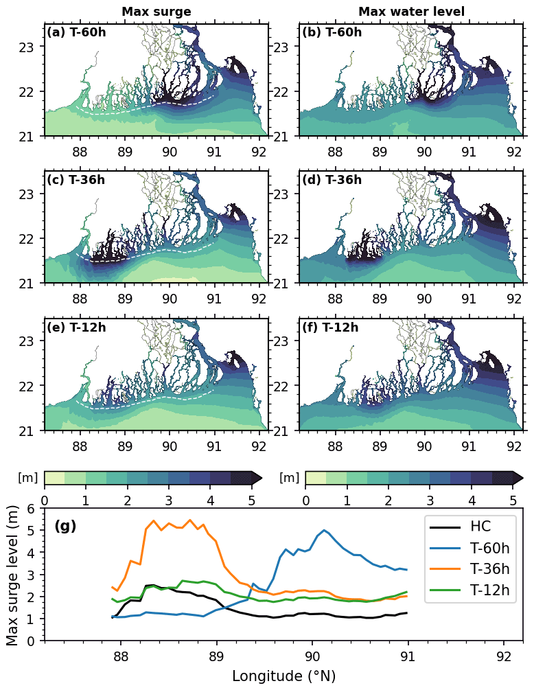
Figure 8Maximum surge (a, c, e) and elevation (b, d, f) evolution for forecast initiated at (a–b) T−60 h (18 May 2020 00:00 Z), (c–d) T−36 h (19 May 2020 00:00 Z), and (e–f) T−12 (20 May 2020 00:00 Z) hours before landfall. (g) Comparison of maximum surge level extracted along the section shown by the white line in (a), (c), and (e). Hindcast results (HC) is extracted along the same line shown in Fig. 6b.
6.1 Coupled tide–surge–wave dynamics
The water level dynamics over the Bay of Bengal and particularly around the Bengal delta is complex, and the various components of water level have different relative contributions depending on the location. Due to tide–surge interaction, the maximum water level can be lower or higher depending on the tidal phase in a fully non-linear tide–surge coupled simulation compared to its linear counterpart. During Amphan the tide–surge interaction was mostly negative, except within about 10 km of the landfall location. The positive interaction near the landfall location means that the coupled tide–surge estimate was higher than the linearly added tide and surge. In this case, the typical magnitude of tide–surge interaction ranged from −30 to +30 cm. The contribution from the wave-induced set-up along the shoreline increases the maximum water level estimation throughout the coast by about 10 %–15 % during Amphan.
6.2 Performance of storm surge forecasting
Aside from the necessary inclusion of relevant physical processes – tide, surge, waves, and their non-linear interactions – the performance of storm surge forecasting depends on the wind and pressure forcings. The errors in the wind forcing and in the atmospheric pressure forcing are typically the most important ones among the various sources of error in storm surge modelling (Krien et al., 2017). In our forecast environment, the source of this error is twofold – the analytical model used to synthesize the fields from the storm parameters and the numerical weather model used to forecast the storm wind and pressure fields to derive the storm parameters themselves. There have been attempts to find a more accurate formulation from recent satellite scatterometer missions (Krien et al., 2018). However, not one formulation works best in all radial distances from the storm centre. Despite the well-known error associated with the parametric wind field, they are widely used in applications due to their computational simplicity and lightweight data requirements (Lin and Chavas, 2012). The best way to avoid the error from the analytical wind field might be not using these formulations and relying instead on the full-fledged atmospheric forecasts. However, atmospheric models are costly in terms of computation. It is particularly true for cyclonic storms where high spatial resolution (typically kilometric) is required (Tallapragada et al., 2014).
From the validation of water level at a few tide gauge locations for our hindcast simulation, it appears that the modelling framework proposed here could capture the maximum surge level successfully throughout the coast. Our tide gauge sites were limited to the eastern side of the Amphan landfall location and were operational throughout the life cycle of the cyclone. However, it was not possible to confirm the ability of the model to reproduce the water level on the western side of the landfall location due to data unavailability. The proper reproduction of the maximum water level by the model gives strong confidence in the formulation as well as in the coupling strategy of our modelling framework.
6.3 Inundation
One of the potential, but challenging, outcomes of storm surge forecasting is the prediction of inundation. Particularly in the northern Bay of Bengal, the existing modelling studies do not generally consider the inundation process (Dube et al., 2004; Murty et al., 2014). Some modelling systems take advantage of simplified inundation modelling schemes to tackle this problem (Lewis et al., 2013). In our modelling framework, the inland inundation is calculated seamlessly by SCHISM, solving the same hydrodynamics over the model domain, thanks to the combination of a cross-scale unstructured grid and an efficient wetting–drying algorithm. While the recent improvements in model bathymetry and the detailed accounting of dikes and coastal defences improved the overall modelling of the inundation, the associated error remains large (Krien et al., 2017). As an update to Krien et al. (2017), in our model we have incorporated a novel dike height dataset bearing varying dike crest heights for the numerous polders scattered around the Bengal delta. The assessment of the impact of the updated embankment heights is, however, hard to quantify and validate.

Figure 9Digitized location of inundation resulting from embankment breaching (red), flooding of low-lying unembanked area (orange), and embankment overflow (cyan) overlaid on a false-colour image composite derived from B12, B11, and B4 channels of Sentinel-2 during April 2020. The grey patches are the inundated regions predicted by the model, as shown in the hindcast experiment. The polders are shown with cyan outlines.
In the absence of any operational network of inundation monitoring, to understand and better characterize the inundation dynamics, we systematically skimmed the Bengal delta local newspapers on the day of Amphan landfall and on the few subsequent days to achieve an as-comprehensive-as-possible mapping of the inundation extent observed in situ. We digitized the reported flooded locations through © Google Earth and categorized the inundation mechanism. We digitized 88 such locations over the Bangladeshi part of the Bengal delta, as shown in Fig. 9 (Khan, 2020). Over the Indian side of the delta, the news reporting of inland flooding from dike breaching was not accurate enough for us to be able to geotag the locations. We overlaid the inundated locations over the inundation predicted by the model on a false-colour image derived from the Sentinel-2 satellite using © Google Earth Engine (https://earthengine.google.com, last access: 25 June 2020). Three categories of inundation mechanism are typically observed – inundation by breaching of the dikes (labelled as “embankment breach”), inundation of unprotected low land by increased water level (“unembanked lowland”), and flooding by overflowing of the dikes (“embankment overflow”). From the reported news, it is clear that the major part of the inundation results from the breaching of dikes. We also note two breaching instances in the south-eastern corner of our domain, very far from the cyclone landfall. On the other hand, the flooding from merely increased water level in non-diked areas is mostly concentrated along the Meghna estuary. Along the estuary, designed embankments probably do not exist to protect many populated low-lying char areas (land or island formed though accretion). We could find only one report of the occurrence of overflowing of an embankment, in Maheshwaripur of Koyra Upazila (22.45∘ N, 89.30∘ E). Around 22.4–22.6∘ N, 90.1–90.5∘ E, in Barishal district, our model predicted an extended inundated area, which is known to not be polderized. While we could find some reports of flooding around that region from our newspaper survey, the widespread inundation predicted by our model in this region probably did not occur in reality due to the presence of levees and city protection embankments. Indeed, this kind of small-scale geographic information, to the best of our knowledge, is not systematically available publicly and thus could not be incorporated in our model topography, despite being of utmost importance for localized inundation forecasting. The forecast flooded vs. non-flooded areas show a wealth of spatial scales, demonstrating that our unstructured modelling framework has the intrinsic capability to model the small-scale hydrodynamic gradients. In our modelled forecasts, the contrast between the well-predicted water level temporal evolution and the comparatively limited predictive skills of inundated locations points out the necessity of accurate knowledge and incorporation of reliable topographic and embankment information at the local scale. Our modelling system has the ability and appropriate resolution to ingest such topographic information efficiently due to its unstructured nature.
The coastal polder management has long been a boon and a bane (Warner et al., 2018). On one side, the polders have protected the fertile areas from daily tidal flooding of brackish waters, which favoured agricultural production by reducing the soil salinity (Nowreen et al., 2013). On the other hand, these embankments have restricted fresh water and sediment supply, causing significant subsidence inside the embanked areas due to sediment compaction (Auerbach et al., 2015). Over time, the land use inside these polders has also changed from agriculture to aquaculture (namely shrimp and crab farming). Although the embankments were not built to protect from the cyclonic surges, in many instances they functioned as such. The presence of these protective structures also contributed to a false sense of security among the residents living inside (Paul and Dutt, 2010). Embankments have become part and parcel of survival in this low-lying region. It has now become essential to monitor the condition and topography of the embankments for efficient management and maintenance. From a forecasting point of view, embankment breaching is extremely hard to model in the state-of-the-art hydrodynamic modelling frameworks. However, consistent periodic monitoring of the embankment conditions can improve the forecast by providing a more objective view of the associated inundation hazard.
6.4 Prospects in operational forecasting
Throughout our forecast and hindcast experiments, we have relied on freely available forecast products as the forcing for our storm surge model. These forecasts data are publicly available within 3 h of their initialization time through online portals. The primary input to generate the forcing is the forecast storm track distributed as a text file, which is very lightweight even for a limited internet connection. We have implemented our storm surge model on a freely available open-source framework. The model code is already operationally used in regional forecasting systems and services (Fortunato et al., 2017; Oliveira et al., 2020).
As we have demonstrated, the modelling set-up presented here is tractable in an operational, real-time forecasting scenario. Thanks to advanced and efficient numerics, one can deploy such a system in a consumer-grade computing environment. The computing set-up we have deliberately used (see Table 2) essentially amounts to a high-end x86-64 personal desktop computer (e.g. Intel® Core™ i9-10900 or similar). This computing requirement takes only a portion of the available computing capacity of an institute such as the BMD (15×4 cores at 2.8 GHz) (Roy et al., 2015). Furthermore, the model is easily deployable in a cloud computing infrastructure (Oliveira et al., 2020), which could provide additional reliability and cost savings for an event-driven operational forecasting system.
In this study, we present a retrospective evaluation of storm surge prediction during Supercyclone Amphan using an efficient, state-of-the-art coupled hydrodynamics–wave numerical model. During Cyclone Amphan, the predicted maximum water level ranges from 2 to 5 m along the coastline. Comparison with in situ measurements revealed that the water level could be modelled with high accuracy on the condition that all the relevant mechanisms are considered. Notably, we demonstrated the necessity of considering a coupled hydrodynamic tide–surge–wave modelling framework for the head of the Bay of Bengal for effective forecasting. For Amphan, the contribution from tide–surge interaction and wave set-up typically amounts to 10 % and 10 %–15 % of the total water level, respectively.
From our proactive forecast initiative during Cyclone Amphan, we showed that with publicly available storm forecast products and easily accessible computing resources, it is feasible to forecast the evolution of water level throughout the vast coastline of the Bengal delta in real time. During Amphan, a sufficiently skilful storm surge forecast was achieved as early as 36–48 h before landfall. The forecast water level with 36 h lead time seemed quite similar to our hindcast (HC) simulation in terms of maximum water level as well as the spatial pattern. We communicated the results to the Bangladesh local government authority through personal communications as well as to the scientific community through social media.
From a secondary post-disaster news survey, we have identified the limiting factors for location-specific inundation forecasts. The main limiting factor is due to limited and outdated topographic information of the existing coastal defences. Also, dike breaching, which was the prevalent process of inland inundation during Amphan, is not explicitly modelled in our hydrodynamic framework. These two factors call for routine monitoring of embankment topography and condition.
Cyclone and storm surge warning has always been a communication and trust issue in the Bay of Bengal (Paul and Dutt, 2010; Roy et al., 2015). It is thus necessary to communicate well-grounded storm and surge forecasts to the community for coordinated and informed decision-making during a storm surge (Morss et al., 2018). The forecasting system we implemented and assessed in the present case study provides the proof of feasibility and opens short-term operational prospects to fill a gap in the existing disaster management tools in this part of the world.
The instructions to download and install the model used in this study can be accessed freely at https://github.com/schism-dev/schism (SCHISM development team, 2020). The sources of the data used in this study are described in Sects. 4 and 5 of the article. The data should be requested through the mentioned institutions or downloaded from the provided websites. The geolocation of inundation mapping from newspapers can be found at https://doi.org/10.5281/zenodo.4086102 (Khan, 2020).
The supplement related to this article is available online at: https://doi.org/10.5194/nhess-21-2523-2021-supplement.
MJUK and FD formulated the study. MJUK did the numerical simulations and analysis and wrote the first draft. XB computed the simulation for the WW3 boundary used in the hindcast. All co-authors contributed to this study through multiple discussions. MP provided help with the WWM formulation. SH disseminated the forecasts to the local government of Bangladesh and AKMSI to the scientific community during Cyclone Amphan.
The authors declare that they have no conflict of interest.
Publisher’s note: Copernicus Publications remains neutral with regard to jurisdictional claims in published maps and institutional affiliations.
We are thankful to the LIENSs Laboratory (University of La Rochelle, France) for hosting Md. Jamal Uddin Khan and Laurent Testut during this study.
This research has been supported by the Centre National d'Etudes Spatiales (TOSCA BANDINO grant), the embassy of France in Bangladesh, and the Agence Nationale de la Recherche (DELTA grant no. ANR-17-CE03-0001).
This paper was edited by Animesh Gain and reviewed by two anonymous referees.
Ahsan, M. N., Khatun, A., Islam, M. S., Vink, K., Ohara, M., and Fakhruddin, B. S.: Preferences for improved early warning services among coastal communities at risk in cyclone prone south-west region of Bangladesh, Progress in Disaster Science, 5, 100065, https://doi.org/10.1016/j.pdisas.2020.100065, 2020. a
Alam, E. and Dominey-Howes, D.: A new catalogue of tropical cyclones of the northern Bay of Bengal and the distribution and effects of selected landfalling events in Bangladesh, Int. J. Climatol., 35, 801–835, https://doi.org/10.1002/joc.4035, 2014. a, b
Ali, A.: Climate change impacts and adaptation assessment in Bangladesh, Clim. Res., 12, 109–116, https://doi.org/10.3354/cr012109, 1999. a, b
Antony, C. and Unnikrishnan, A. S.: Observed characteristics of tide-surge interaction along the east coast of India and the head of Bay of Bengal, Estuar. Coast. Shelf S., 131, 6–11, https://doi.org/10.1016/j.ecss.2013.08.004, 2013. a, b
Antony, C., Unnikrishnan, A., Krien, Y., Murty, P., Samiksha, S., and Islam, A.: Tide–surge interaction at the head of the Bay of Bengal during Cyclone Aila, Regional Studies in Marine Science, 35, 101133, https://doi.org/10.1016/j.rsma.2020.101133, 2020. a
Ardhuin, F., Rogers, E., Babanin, A. V., Filipot, J.-F., Magne, R., Roland, A., van der Westhuysen, A., Queffeulou, P., Lefevre, J.-M., Aouf, L., and Collard, F.: Semiempirical Dissipation Source Functions for Ocean Waves. Part I: Definition, Calibration, and Validation, J. Phys. Oceanogr., 40, 1917–1941, https://doi.org/10.1175/2010jpo4324.1, 2010. a
As-Salek, J. A. and Yasuda, T.: Tide–Surge Interaction in the Meghna Estuary: Most Severe Conditions, J. Phys. Oceanogr., 31, 3059–3072, https://doi.org/10.1175/1520-0485(2001)031<3059:tsiitm>2.0.co;2, 2001. a, b, c
Auerbach, L. W., Jr, S. L. G., Mondal, D. R., Wilson, C. A., Ahmed, K. R., Roy, K., Steckler, M. S., Small, C., Gilligan, J. M., and Ackerly, B. A.: Flood risk of natural and embanked landscapes on the Ganges–Brahmaputra tidal delta plain, Nat. Clim. Change, 5, 153–157, https://doi.org/10.1038/nclimate2472, 2015. a, b
Battjes, J. A. and Janssen, J. P. F. M.: Energy Loss and Set-Up Due to Breaking of Random Waves, in: Coastal Engineering 1978, American Society of Civil Engineers, Hamburg, Germany, 569–587, https://doi.org/10.1061/9780872621909.034, 1978. a
Bernier, N. B. and Thompson, K. R.: Deterministic and ensemble storm surge prediction for Atlantic Canada with lead times of hours to ten days, Ocean Model., 86, 114–127, https://doi.org/10.1016/j.ocemod.2014.12.002, 2015. a
Bertin, X., Li, K., Roland, A., Zhang, Y. J., Breilh, J. F., and Chaumillon, E.: A modeling-based analysis of the flooding associated with Xynthia, central Bay of Biscay, Coast. Eng., 94, 80–89, https://doi.org/10.1016/j.coastaleng.2014.08.013, 2014. a, b
Bertin, X., Li, K., Roland, A., and Bidlot, J.-R.: The contribution of short-waves in storm surges: Two case studies in the Bay of Biscay, Cont. Shelf Res., 96, 1–15, https://doi.org/10.1016/j.csr.2015.01.005, 2015. a, b
Bhardwaj, P. and Singh, O.: Climatological characteristics of Bay of Bengal tropical cyclones: 1972–2017, Theor. Appl. Climatol., 139, 615–629, https://doi.org/10.1007/s00704-019-02989-4, 2019. a
Bouwer, L. M. and Jonkman, S. N.: Global mortality from storm surges is decreasing, Environ. Res. Lett., 13, 014008, https://doi.org/10.1088/1748-9326/aa98a3, 2018. a
Carrère, L., Lyard, F., Cancet, M., Guillot, A., and Roblou, L.: FES 2012: a new global tidal model taking advantage of nearly 20 years of altimetry, in: 20 Years of Progress in Radar Altimatry, European Space Agency, Venice, Italy, vol. 710, 2013. a, b
Center For International Earth Science Information Network (CIESIN), Columbia University: Documentation for Gridded Population of the World, Version 4 (GPWv4), https://doi.org/10.7927/H4D50JX4, 2016. a
Chowdhury, M. A. M. and Al Rahim, M.: A proposal on new scheduling of turbine discharge at Kaptai hydro-electric power plant to avoid the wastage of water due to overflow in the dam, in: 2012 7th International Conference on Electrical and Computer Engineering, IEEE, 758–762, 2012. a
Condon, A. J., Sheng, Y. P., and Paramygin, V. A.: Toward High-Resolution, Rapid, Probabilistic Forecasting of the Inundation Threat from Landfalling Hurricanes, Mon. Weather Rev., 141, 1304–1323, https://doi.org/10.1175/mwr-d-12-00149.1, 2013. a
Daniel, P., Haie, B., and Aubail, X.: Operational Forecasting of Tropical Cyclones Storm Surges at Meteo-France, Mar. Geod., 32, 233–242, https://doi.org/10.1080/01490410902869649, 2009. a
Das, P. K.: Prediction Model for Storm Surges in the Bay of Bengal, Nature, 239, 211–213, https://doi.org/10.1038/239211a0, 1972. a
Deb, M. and Ferreira, C. M.: Simulation of cyclone-induced storm surges in the low-lying delta of Bangladesh using coupled hydrodynamic and wave model (SWAN + ADCIRC), J. Flood Risk Manag., 11, S750–S765, https://doi.org/10.1111/jfr3.12254, 2016. a, b
DhakaTribune: Govt: Cyclone caused damage worth Tk1, 100 crore, https://www.dhakatribune.com/bangladesh/crisis/2020/05/21/govt-estimated-damages-from-amphan-worth-1-100-crore last access: 22 May 2020. a
Dube, S. K., Chittibabu, P., Sinha, P. C., Rao, A. D., and Murty, T. S.: Numerical Modelling of Storm Surge in the Head Bay of Bengal Using Location Specific Model, Nat. Hazards, 31, 437–453, https://doi.org/10.1023/b:nhaz.0000023361.94609.4a, 2004. a, b
Dube, S. K., Jain, I., Rao, A. D., and Murty, T. S.: Storm surge modelling for the Bay of Bengal and Arabian Sea, Nat. Hazards, 51, 3–27, https://doi.org/10.1007/s11069-009-9397-9, 2009. a, b
Durand, F., Piecuch, C. G., Becker, M., Papa, F., Raju, S. V., Khan, J. U., and Ponte, R. M.: Impact of Continental Freshwater Runoff on Coastal Sea Level, Surv. Geophys., 40, 1437–1466, https://doi.org/10.1007/s10712-019-09536-w, 2019. a
Egbert, G. D. and Erofeeva, S. Y.: Efficient inverse modeling of barotropic ocean tides, J. Atmos. Ocean. Tech., 19, 183–204, 2002. a
Emanuel, K.: Increasing destructiveness of tropical cyclones over the past 30 years, Nature, 436, 686–688, https://doi.org/10.1038/nature03906, 2005. a
Emanuel, K. and Rotunno, R.: Self-Stratification of Tropical Cyclone Outflow. Part I: Implications for Storm Structure, J. Atmos. Sci., 68, 2236–2249, https://doi.org/10.1175/jas-d-10-05024.1, 2011. a
Fernández-Montblanc, T., Vousdoukas, M., Ciavola, P., Voukouvalas, E., Mentaschi, L., Breyiannis, G., Feyen, L., and Salamon, P.: Towards robust pan-European storm surge forecasting, Ocean Model., 133, 129–144, https://doi.org/10.1016/j.ocemod.2018.12.001, 2019. a, b
Flather, R. A.: A Storm Surge Prediction Model for the Northern Bay of Bengal with Application to the Cyclone Disaster in April 1991, J. Phys. Oceanogr., 24, 172–190, https://doi.org/10.1175/1520-0485(1994)024<0172:asspmf>2.0.co;2, 1994. a
Flowerdew, J., Mylne, K., Jones, C., and Titley, H.: Extending the forecast range of the UK storm surge ensemble, Q. J. Roy. Meteor. Soc., 139, 184–197, https://doi.org/10.1002/qj.1950, 2012. a
Fortunato, A. B., Oliveira, A., Rogeiro, J., Tavares da Costa, R., Gomes, J. L., Li, K., de Jesus, G., Freire, P., Rilo, A., Mendes, A., Rodrigues, M., and Azevedo, A.: Operational forecast framework applied to extreme sea levels at regional and local scales, J. Oper. Oceanogr., 10, 1–15, https://doi.org/10.1080/1755876X.2016.1255471, 2017. a, b, c
Frank, N. L. and Husain, S.: The deadliest tropical cyclone in history?, B. Am. Meteorol. Soc., 52, 438–445, 1971. a
Glahn, B., Taylor, A., Kurkowski, N., and Shaffer, W.: The role of the SLOSH model in National Weather Service storm surge forecasting, National Weather Digest, 33, 3–14, 2009. a, b
Guérin, T., Bertin, X., Coulombier, T., and de Bakker, A.: Impacts of wave-induced circulation in the surf zone on wave setup, Ocean Model., 123, 86–97, https://doi.org/10.1016/j.ocemod.2018.01.006, 2018. a, b
Holland, G. J.: An Analytic Model of the Wind and Pressure Profiles in Hurricanes, Mon. Weather Rev., 108, 1212–1218, https://doi.org/10.1175/1520-0493(1980)108<1212:aamotw>2.0.co;2, 1980. a
Idier, D., Bertin, X., Thompson, P., and Pickering, M. D.: Interactions Between Mean Sea Level, Tide, Surge, Waves and Flooding: Mechanisms and Contributions to Sea Level Variations at the Coast, Surv. Geophys., 40, 1603–1630, https://doi.org/10.1007/s10712-019-09549-5, 2019. a, b
IFRC: Operation Update Report, http://adore.ifrc.org/Download.aspx?FileId=329843 (last access: 22 February 2021), 2020a. a, b
IFRC: Bangladesh: Cyclone – Final report early action, https://reliefweb.int/sites/reliefweb.int/files/resources/EAP2018BD01fr.pdf (last access: 22 February 2021) 2020b. a
IMD: Super Cyclonic Storm “AMPHAN” over the southeast Bay of Bengal (16th–21st May 2020): A Report, Tech. rep., Cyclone Warning Division – India Meteorological Department, New Delhi, available at: https://www.rsmcnewdelhi.imd.gov.in/uploads/report/26/26_936e63_amphan.pdf, last access: 27 July 2021. a
Islam, A. S., Bala, S. K., Hussain, M. A., Hossain, M. A., and Rahman, M. M.: Performance of Coastal Structures during Cyclone Sidr, Nat. Hazards Rev., 12, 111–116, https://doi.org/10.1061/(asce)nh.1527-6996.0000031, 2011. a
Ji, M., Aikman, F., and Lozano, C.: Toward improved operational surge and inundation forecasts and coastal warnings, Nat. Hazards, 53, 195–203, https://doi.org/10.1007/s11069-009-9414-z, 2009. a
Johns, B. and Ali, M. A.: The numerical modelling of storm surges in the Bay of Bengal, Q. J. Roy. Meteor. Soc., 106, 1–18, https://doi.org/10.1002/qj.49710644702, 1980. a, b, c
Khalid, A. and Ferreira, C.: Advancing real-time flood prediction in large estuaries: iFLOOD a fully coupled surge-wave automated web-based guidance system, Environ. Modell. Softw., 131, 104748, https://doi.org/10.1016/j.envsoft.2020.104748, 2020. a, b
Khalil, G. M.: The catastrophic cyclone of April 1991: Its Impact on the economy of Bangladesh, Nat. Hazards, 8, 263–281, https://doi.org/10.1007/bf00690911, 1993. a
Khan, M. J. U.: Digitized flood location dataset during cyclone Amphan from newspaper survey, Zenodo [data set], https://doi.org/10.5281/ZENODO.4086102, 2020. a, b
Khan, M. J. U., Ansary, M. N., Durand, F., Testut, L., Ishaque, M., Calmant, S., Krien, Y., Islam, A. K. M. S., and Papa, F.: High-Resolution Intertidal Topography from Sentinel-2 Multi-Spectral Imagery: Synergy between Remote Sensing and Numerical Modeling, Remote Sensing, 11, 2888, https://doi.org/10.3390/rs11242888, 2019. a, b, c
Krien, Y., Mayet, C., Testut, L., Durand, F., Tazkia, A. R., Islam, A. K. M. S., Gopalakrishna, V. V., Becker, M., Calmant, S., Shum, C. K., Khan, Z. H., Papa, F., and Ballu, V.: Improved Bathymetric Dataset and Tidal Model for the Northern Bay of Bengal, Mar. Geodesy, 39, 422–438, https://doi.org/10.1080/01490419.2016.1227405, 2016. a, b, c, d
Krien, Y., Testut, L., Islam, A. K. M. S., Bertin, X., Durand, F., Mayet, C., Tazkia, A. R., Becker, M., Calmant, S., Papa, F., Ballu, V., Shum, C. K., and Khan, Z. H.: Towards improved storm surge models in the northern Bay of Bengal, Cont. Shelf Res., 135, 58–73, https://doi.org/10.1016/j.csr.2017.01.014, 2017. a, b, c, d, e, f, g, h, i, j, k, l, m, n, o, p
Krien, Y., Arnaud, G., Cécé, R., Ruf, C., Belmadani, A., Khan, J., Bernard, D., Islam, A. K. M. S., Durand, F., Testut, L., Palany, P., and Zahibo, N.: Can We Improve Parametric Cyclonic Wind Fields Using Recent Satellite Remote Sensing Data?, Remote Sensing, 10, 1963, https://doi.org/10.3390/rs10121963, 2018. a, b, c
Kumar, T. S., Murty, P., Kumar, M. P., Kumar, M. K., Padmanabham, J., Kumar, N. K., Shenoi, S., Mohapatra, M., Nayak, S., and Mohanty, P.: Modeling Storm Surge and its Associated Inland Inundation Extent Due to Very Severe Cyclonic Storm Phailin, Mar. Geod., 38, 345–360, https://doi.org/10.1080/01490419.2015.1053640, 2015. a
Kuroda, T., Saito, K., Kunii, M., and Kohno, N.: Numerical Simulations of Myanmar Cyclone Nargis and the Associated Storm Surge Part I: Forecast Experiment with a Nonhydrostatic Model and Simulation of Storm Surge, J. Meteorol. Soc. JPN, 88, 521–545, https://doi.org/10.2151/jmsj.2010-315, 2010. a, b
Lane, E. M., Walters, R. A., Gillibrand, P. A., and Uddstrom, M.: Operational forecasting of sea level height using an unstructured grid ocean model, Ocean Model., 28, 88–96, https://doi.org/10.1016/j.ocemod.2008.11.004, 2009. a, b
Lazo, J. K. and Waldman, D. M.: Valuing improved hurricane forecasts, Econ. Lett., 111, 43–46, https://doi.org/10.1016/j.econlet.2010.12.012, 2011. a
Lazo, J. K., Bostrom, A., Morss, R. E., Demuth, J. L., and Lazrus, H.: Factors Affecting Hurricane Evacuation Intentions, Risk Anal., 35, 1837–1857, https://doi.org/10.1111/risa.12407, 2015. a
Lewis, M., Bates, P., Horsburgh, K., Neal, J., and Schumann, G.: A storm surge inundation model of the northern Bay of Bengal using publicly available data, Q. J. Roy. Meteorol. Soc., 139, 358–369, https://doi.org/10.1002/qj.2040, 2013. a
Lin, N. and Chavas, D.: On hurricane parametric wind and applications in storm surge modeling, J. Geophys. Res.-Atmos., 117, D09120, https://doi.org/10.1029/2011jd017126, 2012. a, b
Loftis, J. D., Mitchell, M., Schatt, D., Forrest, D. R., Wang, H. V., Mayfield, D., and Stiles, W. A.: Validating an Operational Flood Forecast Model Using Citizen Science in Hampton Roads, VA, USA, Journal of Marine Science and Engineering, 7, 242, https://doi.org/10.3390/jmse7080242, 2019. a
Longuet-Higgins, M. S. and Stewart, R. w.: Radiation stresses in water waves; a physical discussion, with applications, Deep Sea Research and Oceanographic Abstracts, 11, 529–562, https://doi.org/10.1016/0011-7471(64)90001-4, 1962. a
Madsen, H. and Jakobsen, F.: Cyclone induced storm surge and flood forecasting in the northern Bay of Bengal, Coastal Eng., 51, 277–296, https://doi.org/10.1016/j.coastaleng.2004.03.001, 2004. a
Magnusson, L., Bidlot, J.-R., Bonavita, M., Brown, A. R., Browne, P. A., Chiara, G. D., Dahoui, M., Lang, S. T. K., McNally, T., Mogensen, K. S., Pappenberger, F., Prates, F., Rabier, F., Richardson, D. S., Vitart, F., and Malardel, S.: ECMWF Activities for Improved Hurricane Forecasts, B. Am. Meteorol. Soc., 100, 445–458, https://doi.org/10.1175/bams-d-18-0044.1, 2019. a
Melton, G., Gall, M., Mitchell, J. T., and Cutter, S. L.: Hurricane Katrina storm surge delineation: implications for future storm surge forecasts and warnings, Nat. Hazards, 54, 519–536, https://doi.org/10.1007/s11069-009-9483-z, 2009. a
Miller, R. J., Schrader, A. J., Sampson, C. R., and Tsui, T. L.: The Automated Tropical Cyclone Forecasting System (ATCF), Weather Forecast., 5, 653–660, https://doi.org/10.1175/1520-0434(1990)005<0653:tatcfs>2.0.co;2, 1990. a
Morss, R. E., Cuite, C. L., Demuth, J. L., Hallman, W. K., and Shwom, R. L.: Is storm surge scary? The influence of hazard, impact, and fear-based messages and individual differences on responses to hurricane risks in the USA, Int. J. Disast. Risk Red., 30, 44–58, https://doi.org/10.1016/j.ijdrr.2018.01.023, 2018. a
Mukhopadhyay, S., Biswas, H., De, T., and Jana, T.: Fluxes of nutrients from the tropical River Hooghly at the land–ocean boundary of Sundarbans, NE Coast of Bay of Bengal, India, J. Marine Syst., 62, 9–21, https://doi.org/10.1016/j.jmarsys.2006.03.004, 2006. a
Munroe, R., Montz, B., and Curtis, S.: Getting More out of Storm Surge Forecasts: Emergency Support Personnel Needs in North Carolina, Weather Clim. Soc., 10, 813–820, https://doi.org/10.1175/wcas-d-17-0074.1, 2018. a
Murty, P. L. N., Sandhya, K. G., Bhaskaran, P. K., Jose, F., Gayathri, R., Nair, T. M. B., Kumar, T. S., and Shenoi, S. S. C.: A coupled hydrodynamic modeling system for PHAILIN cyclone in the Bay of Bengal, Coast. Eng., 93, 71–81, https://doi.org/10.1016/j.coastaleng.2014.08.006, 2014. a, b, c, d
Murty, P. L. N., Bhaskaran, P. K., Gayathri, R., Sahoo, B., Kumar, T. S., and SubbaReddy, B.: Numerical study of coastal hydrodynamics using a coupled model for Hudhud cyclone in the Bay of Bengal, Estuar. Coast. Shelf S., 183, 13–27, https://doi.org/10.1016/j.ecss.2016.10.013, 2016. a, b
Murty, P. L. N., Padmanabham, J., Kumar, T. S., Kumar, N. K., Chandra, V. R., Shenoi, S. S. C., and Mohapatra, M.: Real-time storm surge and inundation forecast for very severe cyclonic storm “Hudhud”, Ocean Eng., 131, 25–35, https://doi.org/10.1016/j.oceaneng.2016.12.026, 2017. a, b, c
Murty, T. S., Flather, R. A., and Henry, R. F.: The storm surge problem in the bay of Bengal, Prog. Oceanogr., 16, 195–233, https://doi.org/10.1016/0079-6611(86)90039-x, 1986. a, b, c, d
National Centers for Environmental Prediction, National Weather Service, NOAA, U.S. Department of Commerce: NCEP GDAS/FNL 0.25 Degree Global Tropospheric Analyses and Forecast Grids, Research Data Archive at the National Center for Atmospheric Research [data set], Computational and Information Systems Laboratory, Boulder CO, https://doi.org/10.5065/D65Q4T4Z, 2015. a
Needham, H. F., Keim, B. D., and Sathiaraj, D.: A review of tropical cyclone-generated storm surges: Global data sources, observations, and impacts, Rev. Geophys., 53, 545–591, https://doi.org/10.1002/2014rg000477, 2015. a, b
Nowreen, S., Jalal, M. R., and Khan, M. S. A.: Historical analysis of rationalizing South West coastal polders of Bangladesh, Water Policy, 16, 264–279, https://doi.org/10.2166/wp.2013.172, 2013. a, b
Oliveira, A., Fortunato, A., Rogeiro, J., Teixeira, J., Azevedo, A., Lavaud, L., Bertin, X., Gomes, J., David, M., Pina, J., Rodrigues, M., and Lopes, P.: OPENCoastS: An open-access service for the automatic generation of coastal forecast systems, Environ. Modell. Softw., 124, 104585, https://doi.org/10.1016/j.envsoft.2019.104585, 2020. a, b, c, d
Paul, B. K.: Why relatively fewer people died? The case of Bangladesh's Cyclone Sidr, Nat. Hazards, 50, 289–304, https://doi.org/10.1007/s11069-008-9340-5, 2009. a
Paul, B. K. and Dutt, S.: Hazard Warnings and Responses to Evacuation Orders: the Case of Bangladesh's Cyclone Sidr, Geogr. Rev., 100, 336–355, https://doi.org/10.1111/j.1931-0846.2010.00040.x, 2010. a, b, c
Pezerat, M., Martins, K., and Bertin, X.: Modelling Storm Waves in the Nearshore Area Using Spectral Models, J. Coastal Res., 95, 1240, https://doi.org/10.2112/SI95-240.1, 2020. a, b
Pezerat, M., Bertin, X., Martins, K., Mengual, B., and Hamm, L.: Simulating storm waves in the nearshore area using spectral model: Current issues and a pragmatic solution, Ocean Model., 158, 101737, https://doi.org/10.1016/j.ocemod.2020.101737, 2021. a, b
Ray, R. D.: A global ocean tide model from TOPEX/POSEIDON altimetry: GOT99. 2, National Aeronautics and Space Administration, Goddard Space Flight Center, 1999. a
Roland, A., Zhang, Y. J., Wang, H. V., Meng, Y., Teng, Y.-C., Maderich, V., Brovchenko, I., Dutour-Sikiric, M., and Zanke, U.: A fully coupled 3D wave-current interaction model on unstructured grids, J. Geophys. Res.-Oceans, 117, C00J33, https://doi.org/10.1029/2012jc007952, 2012. a
Roy, C., Sarkar, S. K., Åberg, J., and Kovordanyi, R.: The current cyclone early warning system in Bangladesh: Providers' and receivers' views, Int. J. Disast. Risk Re., 12, 285–299, https://doi.org/10.1016/j.ijdrr.2015.02.004, 2015. a, b, c
SCHISM development team: SCHISM v5.8, GitHub [code], available at: https://github.com/schism-dev/schism, last access: 15 May 2020. a
Schmidt, S., Kemfert, C., and Höppe, P.: Tropical cyclone losses in the USA and the impact of climate change – A trend analysis based on data from a new approach to adjusting storm losses, Environmental Impact Assessment Review, 29, 359–369, https://doi.org/10.1016/j.eiar.2009.03.003, 2009. a
Seo, S. N. and Bakkensen, L. A.: Is Tropical Cyclone Surge, Not Intensity, What Kills So Many People in South Asia?, Weather Clim. Soc., 9, 171–181, https://doi.org/10.1175/wcas-d-16-0059.1, 2017. a
Suh, S. W., Lee, H. Y., Kim, H. J., and Fleming, J. G.: An efficient early warning system for typhoon storm surge based on time-varying advisories by coupled ADCIRC and SWAN, Ocean Dynam., 65, 617–646, https://doi.org/10.1007/s10236-015-0820-3, 2015. a, b
Tallapragada, V., Kieu, C., Kwon, Y., Trahan, S., Liu, Q., Zhang, Z., and Kwon, I.-H.: Evaluation of Storm Structure from the Operational HWRF during 2012 Implementation, Mon. Weather Rev., 142, 4308–4325, https://doi.org/10.1175/MWR-D-13-00010.1, 2014. a, b
Tazkia, A. R., Krien, Y., Durand, F., Testut, L., Islam, A. S., Papa, F., and Bertin, X.: Seasonal modulation of M2 tide in the Northern Bay of Bengal, Cont. Shelf Res., 137, 154–162, https://doi.org/10.1016/j.csr.2016.12.008, 2017. a, b
Verlaan, M., Zijderveld, A., Vries, H. d., and Kroos, J.: Operational storm surge forecasting in the Netherlands: developments in the last decade, Philosophical Transactions of the Royal Society A: Mathematical, Phys. Eng. Sci., 363, 1441–1453, https://doi.org/10.1098/rsta.2005.1578, 2005. a
Warner, J. F., van Staveren, M. F., and van Tatenhove, J.: Cutting dikes, cutting ties? Reintroducing flood dynamics in coastal polders in Bangladesh and the netherlands, Int. J. Disast. Risk Re., 32, 106–112, https://doi.org/10.1016/j.ijdrr.2018.03.020, 2018. a
WW3DG: User manual and system documentation of WAVEWATCH III TM, GitHub [code], available at: https://github.com/NOAA-EMC/WW3 (last access: 30 May 2020), 2019. a
Yang, K., Paramygin, V. A., and Sheng, Y. P.: A Rapid Forecasting and Mapping System of Storm Surge and Coastal Flooding, Weather Forecast., 35, 1663–1681, https://doi.org/10.1175/WAF-D-19-0150.1, 2020. a
Ye, F., Zhang, Y. J., Yu, H., Sun, W., Moghimi, S., Myers, E., Nunez, K., Zhang, R., Wang, H. V., Roland, A., Martins, K., Bertin, X., Du, J., and Liu, Z.: Simulating storm surge and compound flooding events with a creek-to-ocean model: Importance of baroclinic effects, Ocean Model., 145, 101526, https://doi.org/10.1016/j.ocemod.2019.101526, 2020. a
Zhang, Y. and Baptista, A. M.: SELFE: A semi-implicit Eulerian–Lagrangian finite-element model for cross-scale ocean circulation, Ocean Model., 21, 71–96, https://doi.org/10.1016/j.ocemod.2007.11.005, 2008. a
Zhang, Y. J., Stanev, E. V., and Grashorn, S.: Unstructured-grid model for the North Sea and Baltic Sea: Validation against observations, Ocean Model., 97, 91–108, https://doi.org/10.1016/j.ocemod.2015.11.009, 2016a. a
Zhang, Y. J., Ye, F., Stanev, E. V., and Grashorn, S.: Seamless cross-scale modeling with SCHISM, Ocean Model., 102, 64–81, https://doi.org/10.1016/j.ocemod.2016.05.002, 2016b. a
Zhang, Y. J., Ye, F., Yu, H., Sun, W., Moghimi, S., Myers, E., Nunez, K., Zhang, R., Wang, H., Roland, A., Du, J., and Liu, Z.: Simulating compound flooding events in a hurricane, Ocean Dynam., 70, 621–640, https://doi.org/10.1007/s10236-020-01351-x, 2020. a
- Abstract
- Introduction
- Storm surge and inundation processes in the Bay of Bengal
- Atmospheric evolution of Cyclone Amphan
- Storm surge model and performance
- Near-real-time storm surge forecasting
- Discussion
- Conclusions
- Code and data availability
- Author contributions
- Competing interests
- Disclaimer
- Acknowledgements
- Financial support
- Review statement
- References
- Supplement