the Creative Commons Attribution 4.0 License.
the Creative Commons Attribution 4.0 License.
 | 11 Aug 2021
The potential of machine learning for weather index insurance
Luigi Cesarini
Rui Figueiredo
Beatrice Monteleone
Mario L. V. Martina
Weather index insurance is an innovative tool in risk transfer for disasters induced by natural hazards. This paper proposes a methodology that uses machine learning algorithms for the identification of extreme flood and drought events aimed at reducing the basis risk connected to this kind of insurance mechanism. The model types selected for this study were the neural network and the support vector machine, vastly adopted for classification problems, which were built exploring thousands of possible configurations based on the combination of different model parameters. The models were developed and tested in the Dominican Republic context, based on data from multiple sources covering a time period between 2000 and 2019. Using rainfall and soil moisture data, the machine learning algorithms provided a strong improvement when compared to logistic regression models, used as a baseline for both hazards. Furthermore, increasing the amount of information provided during the training of the models proved to be beneficial to the performances, increasing their classification accuracy and confirming the ability of these algorithms to exploit big data and their potential for application within index insurance products.
- Article
(8130 KB) - Full-text XML
- BibTeX
- EndNote


Changes in frequency and severity of extreme weather and climate events have been observed since 1950, including an increase in the number of heavy precipitation events in some land areas and a significant decrease in rainfall in other regions (Field et al., 2014). Impacts from recent weather-related extremes, such as floods and droughts, have revealed a substantial vulnerability of many human systems to climate-related hazards (Visser et al., 2014). In recent decades, extreme weather events have caused widespread economic and social damages all over the world (Kron et al., 2019). According to Hoeppe (2016), over the period from 1980 to 2014, extreme weather events have caused losses of around USD 3300 billion, with floods accounting for 32 % of the losses and drought for 17 %. Extreme weather events have devastating effects on people's lives. The International Disasters Database EMDAT (CRED, 2019) reports that, over the period from 1980 to 2019, extreme weather caused the death of 1.15 million people, with droughts being the disaster responsible for the highest number of deaths (around 50 % of fatalities due to climate extremes), followed by storms (34 %) and floods (16 %).
The implementation of effective disaster risk management strategies is key to limiting economic and social losses associated with extreme weather events and to reducing disaster risk. In recent years, there has been increasing worldwide interest in the integration of risk transfer instruments within such strategies (Kunreuther, 2001; Surminski et al., 2016). Among those instruments, index-based insurance, or parametric insurance, has gained remarkable popularity. Unlike traditional insurance, which indemnifies policyholders based on experienced losses, parametric insurance pays indemnities based on realisations of an index (or a combination of parameters) that is correlated with losses (Barnett and Mahul, 2007). It can be used to transfer risk associated with different types of extreme events, such as earthquakes (Franco, 2010), floods (Surminski and Oramas-Dorta, 2014) and droughts (Makaudze and Miranda, 2010). Parametric insurance offers various advantages over traditional indemnity-based insurance, such as lower operating expenses, reduced moral hazard and adverse selection, and prompt access to funds by the insured following the occurrence of disasters (Ibarra and Skees, 2007; Figueiredo et al., 2018). This promptness is critical in developing countries, which tend to be exposed to short-term liquidity gaps that may overwhelm their capacity to cope with large disasters (Van Nostrand and Nevius, 2011). A critical disadvantage of parametric insurance, however, is its susceptibility to basis risk, which may be defined as the risk that triggered payouts do not coincide with the occurrence of loss events.
The minimisation of basis risk in parametric insurance requires a reliable, rapid and objective identification of extreme climate events. Nowadays, different sources of weather data that may be used to support this endeavour are available. Among them, the use of satellite images and reanalyses products in parametric insurance mechanisms is growing (Black et al., 2016; Chantarat et al., 2013). Satellite images and reanalyses are frequently free of charge, and therefore parametric models based on them are cheaper and can be affordable even for developing countries (Castillo et al., 2016). In addition, satellite images and reanalyses consist of continuous spatial fields and often have global coverage. These last features make them attractive, since they overcome one of the most common issues related to gauges and weather stations, which is their limited or irregular spatial coverage. It should also be noted that, hypothetically, if an entity that is responsible for such stations (e.g. a governmental agency) is related in some form with a potential beneficiary from index insurance coverage, a conflict of interest may arise. This issue is avoided with satellite-based or reanalysis products, which are produced by third parties, for example internationally renowned research institutes such as the Climate Hazards Center of the University of California and the European Centre for Medium-Range Weather Forecasts. Satellite images are often available with high spatial resolution, but records are still short, with a maximum duration of around 30 years. Reanalysis, on the other hand, provides longer time series but tends to have a coarser spatial resolution. Moreover, satellite data should be checked for consistency with ground measurement, which is not always feasible when the network of ground instruments is inadequate or non-existent (Loew et al., 2017). Although using satellite data has its own limitations, various index-based insurance products, exploiting remote-sensing data and reanalysis, have been developed in data-sparse regions such as Africa and Latin America (Awondo, 2018; African Union, 2021; The World Bank, 2008). The combined use of various sources of information to detect the occurrence of extreme events is valuable, since it can significantly improve the ability to correctly detect extreme events (Chiang et al., 2007), and a proper index design helps in addressing the limitations brought by satellite data, as underlined in Black et al. (2016).
Over the last two decades there has been an increasing focus on the application of machine learning methods to process and extract information from big data with limited human intervention (Ornella et al., 2019). Correspondingly, machine learning approaches have also been applied to forecast extreme events. Mosavi et al. (2018) offer an accurate description of the state of the art of machine learning models used to forecast floods, while Hao et al. (2018) and Fung et al. (2019), in their reviews on drought forecasting, give an overview of machine learning tools applied to predict drought indices. Machine learning has also been employed to forecast wind gusts (Sallis et al., 2011), severe hail (Gagne et al., 2017) and excessive rainfall (Nayak and Ghosh, 2013). In contrast, only a minor part of the body of literature focuses its attention on the identification or classification of events (Nayak and Ghosh, 2013, Khalaf et al., 2018, and Alipour et al., 2020, for floods; Richman et al., 2016, for droughts; and Kim et al., 2019 for tropical cyclones). However, classification of events to distinguish between extreme and non-extreme events is essential to support the development of effective parametric risk transfer instruments. In addition, the major part of the analysed studies deals with a single type of event.
This paper aims to assess the potential of machine learning for weather index insurance. To achieve this, we propose and apply a machine learning methodology that is capable of objectively identifying extreme weather events, namely flood and drought, in near-real time, using quasi-global gridded climate datasets derived from satellite imagery or a combination of observation and satellite imagery. The focus of the study is then to address the following research questions.
-
Can machine learning algorithms provide improvement in terms of performance for weather index insurance with respect to traditional approaches?
-
To which extent do the performances of machine learning models improve with the addition of input data?
-
Do the best-performing models share similar properties (e.g. use more input data or consistently have similar algorithm's features)?
In this study we focus on the detection of two types of weather events with very different features: floods, which are mainly local events that can develop over a timescale going from few minutes to days, and droughts, which are creeping phenomena that involve widespread areas and have a slow onset and offset. In addition, floods cause immediate losses (Plate, 2002), while droughts produce non-structural damages and their effects are delayed with respect to the beginning of the event (Wilhite, 2000). Both satellite images and reanalyses are used as input data to show the potential of these instruments when properly designed and managed. Two of the most used machine learning methodologies, neural network (NN) and support vector machine (SVM), are applied. With machine learning (ML) models it is not always straightforward to know a priori which model(s) perform(s) better or which model configuration(s) should be used. Therefore, various model configurations are explored for both NN and SVM, and a rigorous evaluation of their performances is accomplished. The best-performing configurations are tested to reproduce past extreme events in a case study region.
Section 2 describes the NN and SVM algorithms used in this study and their configurations, the procedure adopted to take into consideration the problem of data imbalance due to the rarity of extreme events, the assessment of the quality of the classifications, and the procedure used to select the best-performing models and configurations. In addition, an overview of the datasets used is provided. Section 3 provides some insights on the area where the described methodology is applied. Section 4 presents and discusses the most important outcomes for both floods and droughts. Section 5 summarises the main findings of the study, highlighting their meanings for the study case and analysing the limitations of the proposed approach, while providing insight on possible future developments.
Machine learning is a subset of artificial intelligence whose main purpose is to give computers the possibility to learn, throughout a training process, without being explicitly programmed (Samuel, 1959). It is possible to distinguish machine learning models based on the kind of algorithm that they implement and the type of task that they are required to solve. Algorithms may be divided into two broad groups: the ones using labelled data (Maini and Sabri, 2017), also known as supervised learning algorithms, and the ones that during the training receive only input data for which the output variables are unknown (Ghahramani, 2004), also called unsupervised learning algorithms.
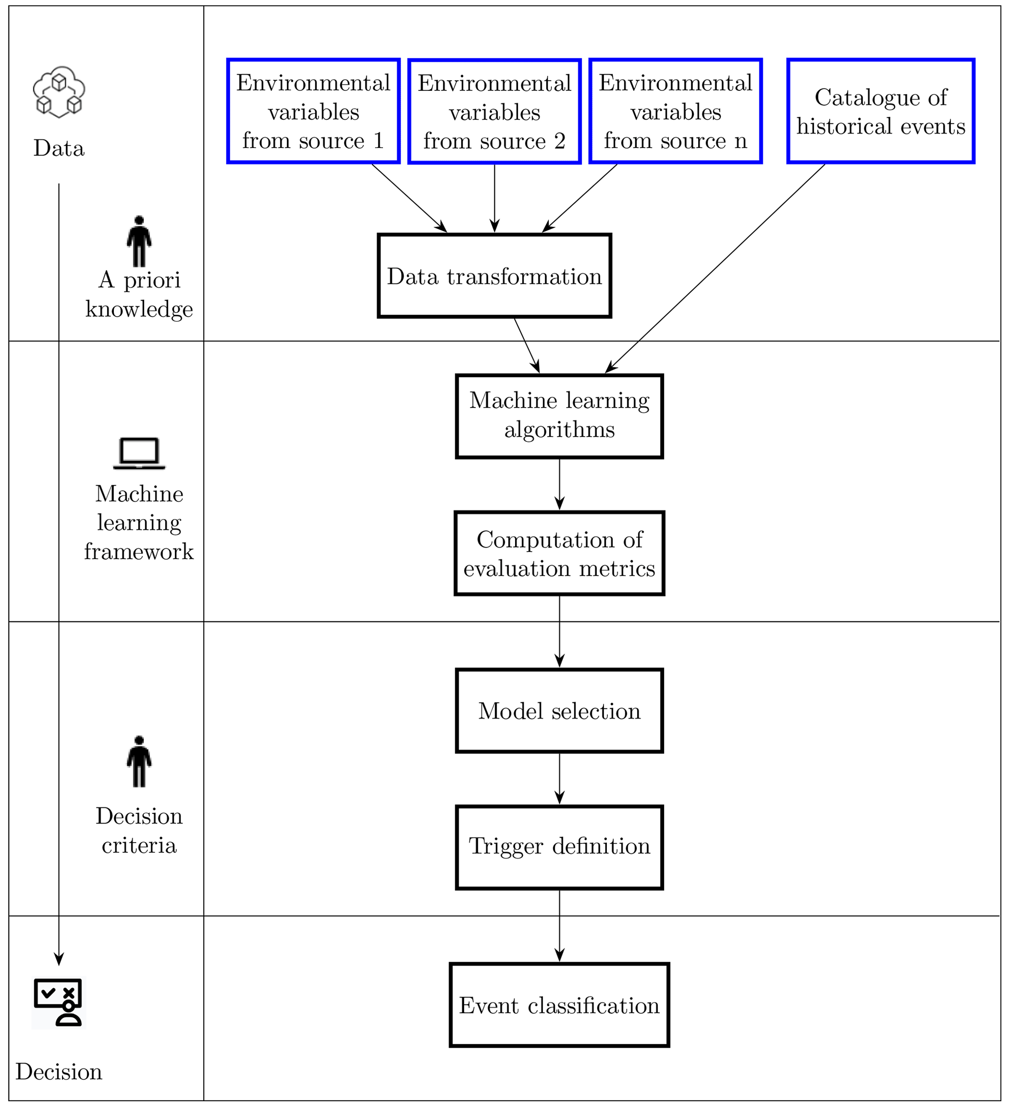
As previously mentioned, in index insurance, payouts are triggered whenever measurable indices exceed predefined thresholds. From a machine learning perspective, this corresponds to an objective classification rule for predicting the occurrence of loss or no loss based on the trigger variable. The rule can be developed using past training sets of hazard and loss data (supervised learning). Conceptually, the development of a parametric trigger should correspond to an informed decision-making process, i.e. a process which, based on data, a priori knowledge and an appropriate modelling framework, can lead to optimal decisions and effective actions. This work aims to leverage the aptitude of machine learning, particularly supervised learning algorithms, to support the decision-making process in the context of parametric risk transfer, applying NN and SVM for the identification of extreme weather events, namely flooding and drought for this particular study.
Consider the occurrence of losses caused by a natural hazard on each time unit over a certain study area G, and let Lt be a binary variable defined as
The aim is then to predict the occurrence of losses based on a set of explanatory variables obtained from non-linear transformations of a set of environmental variables. This hybrid approach aims to capture some of the physical processes of how the hazard creates damage by incorporating a priori expert knowledge on environmental processes and damage-inducing mechanisms for different hazards. Raw environmental variables are not always able to fully describe complex dynamics like flood induced damage; therefore, the usage of expert knowledge is important to provide the machine learning model with input data that are able to better characterise the natural hazard events.
Supervised learning with machine learning methods based on physically motivated transformations of environmental variables are then used to capture loss occurrence. The models are set up such that they produce probabilistic predictions of loss rather than directly classifying events in a binary manner. This allows the parametric trigger to be optimised in a subsequent step, in a metrics-based, objective and transparent manner, by disentangling the construction of the model from the decision-making regarding the definition of the payout-triggering threshold. Probabilistic outputs are also able to provide informative predictions of loss occurrence that convey uncertainty information, which can be useful for end users when a parametric model is operational (Figueiredo et al., 2018).
Figure 1 summarises the general framework implemented in this work.
2.1 Variable and datasets selection
The data-driven nature of ML models implies that the results yielded are as good as the data provided. Thus, the effectiveness of the methods depends heavily on the choice of the input variables, which should be able to represent the underlying physical process (Bowden et al., 2005). The data selection (and subsequent transformation) therefore requires a certain amount of a priori knowledge of the physical system under study. For the purpose of this work, precipitation and soil moisture were used as input variables for both flood and drought. An excessive amount of rainfall is the initial trigger to any flood event (Barredo, 2007), while scarcity of precipitation is one of the main reasons that leads to drought periods (Tate and Gustard, 2000). Soil moisture is instead used as a descriptor of the condition of the soil. With the idea to implement a tool that can be exploited in the framework of parametric risk financing, we selected the datasets to retrieve the two variables according to five criteria.
-
Spatial resolution. A fine spatial resolution that takes into account the climatic features of the various areas of the considered country is needed to develop accurate parametric insurance products.
-
Frequency. The selected datasets should be able to match the duration of the extreme event that we need to identify. For example, in the case of floods, which are quick phenomena, daily or hourly frequencies are required.
-
Spatial coverage. Global spatial coverage enables the extension of the developed approach to areas different from the case study region.
-
Temporal coverage. Since extreme events are rare, a temporal coverage of at least 20 years is considered necessary to allow a correct model calibration.
-
Latency time. A short latency time (i.e. time delay to obtain the most recent data) is necessary to develop tools capable of identifying extreme events in near-real time.
Table 1Main features of the selected (quasi-)global precipitation datasets.
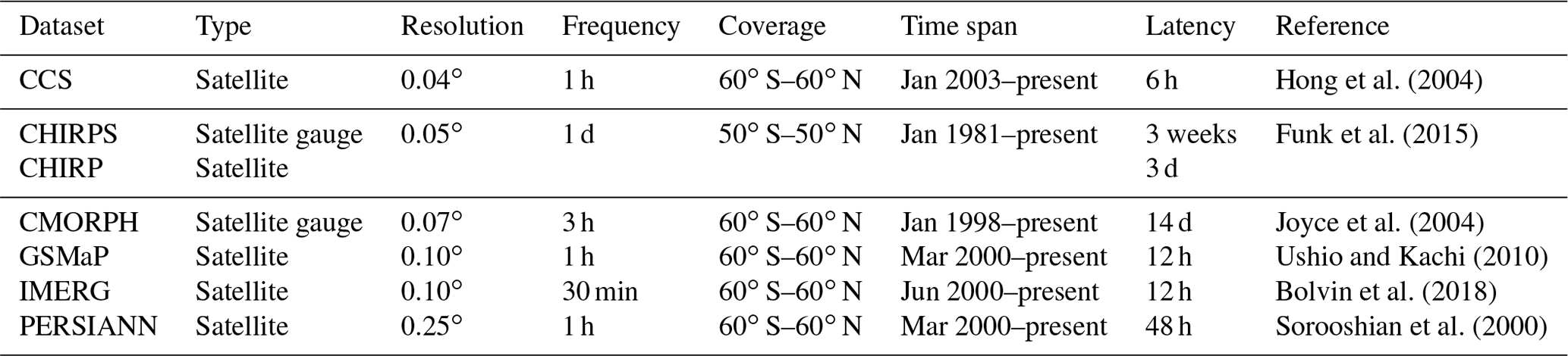
Based on a comprehensive review of available datasets, we found six rainfall datasets and one soil moisture dataset, comprising four layers, matching the above criteria. With respect to the studies analysed in Mosavi et al. (2018), Hao et al. (2018) and Fung et al. (2019), which associated a single dataset to each input variable, here six datasets are associated with a single variable (rainfall). The use of multiple datasets is able to improve the ability of models in identifying extreme events, as demonstrated for example by Chiang et al. (2007) in the case of flash floods. In addition, single datasets may not perform well; the combination of various datasets produces higher-quality estimates (Chen et al., 2019). Two merged satellite-gauge products (the Climate Hazards Group InfraRed Precipitation with Station data, CHIRPS; and the CPC Morphing technique, CMORPH,) and four satellite-only (the Global Satellite Mapping of Precipitation, GSMaP; the Integrated Multi-Satellite Retrievals for GPM, IMERG; the Precipitation Estimation from Remotely Sensed Information using Artificial Neural Networks, PERSIANN; and the global PERSIANN Cloud Classification System, PERSIANN-CCS) datasets were used. The main features of the selected datasets are reported in Table 1.
ECMWF et al. (2018)
Soil moisture was retrieved from the ERA5 reanalysis dataset, produced by the European Centre for Medium Range Weather Forecast (ECMWF). The dataset provides information on four soil moisture layers (layer 1: 0–7 cm, layer 2: 7–28 cm; layer 3: 28–100 cm; layer 4: 100–289 cm). Table 2 shows the main features of the ERA5 dataset.
2.2 Data transformation
The raw environmental variables are subjected to a transformation which is dependent on the hazard at study and is deemed more appropriate to enhance the performances of the model, as described below.
2.2.1 Flood
Flood damage is not directly caused by rainfall but from physical actions originated by water flowing and submerging assets usually located on land. As a result, even if floods are triggered by rainfall, a better predictor for the intensity of a flood and consequent occurrence of damage is warranted. To achieve this, we adopt a variable transformation to emulate, in a simplified manner, the physical processes behind the occurrence of flood damage due to rainfall, based on the approach proposed by Figueiredo et al. (2018), which is now briefly described.
Let Xt(gj) represent the rainfall amount accumulated over grid cell gj belonging to G on day t. Potential runoff is first estimated from daily rainfall. This corresponds to the amount of rainwater that is assumed to not infiltrate the soil and thus remain over the surface and is given by
where u is a constant parameter that represents the daily rate of infiltration.
Overland flow accumulates the excess of rainfall over the surface of a hydrological catchment. This process is modelled using a weighted moving time average, which preserves the accumulation effect and allows the contribution of rainfall on previous days to be considered. The moving average is restricted to a 3 d period. The potential runoff volume accumulated over cell gj over days t, t−1 and t−2 is thus given by
where θ0, θ1, θ2 > 0 and θ0 + θ1 + θ2 = 1.
Finally, let Yt be an explanatory variable representing potential flood intensity for day t, which is defined as
The Box–Cox transformation provides a flexible, non-linear approach to convert runoff to potential damage for each grid cell, which is summed over all grid cells in a study area to obtain a daily index of flood intensity. In order to obtain the Yt variable that best describes potential flood losses due to rainfall, the transformation parameters u, θ1, θ2 and λ are optimised by fitting a logistic regression model to concurrent potential flood intensity and reported occurrences of losses caused by flood events, as well as maximising the likelihood using a quasi-Newton method:
with
2.2.2 Drought
Before being processed by the ML model, rainfall data are used to compute the standardised precipitation index (SPI). The SPI is a commonly used drought index, proposed by McKee et al. (1993). Based on a comparison between the long-term precipitation record (at a given location for a selected accumulation period) and the observed total precipitation amount (for the same accumulation period), the SPI measures the precipitation anomaly. The long-term precipitation record is fitted to the gamma distribution function, which is defined according to the following equation:
where α and β are, respectively, the shape factor and the scale factor. The two parameters are estimated using the maximum likelihood solutions according to the following equations:
where is the mean of the distribution and N is the number of observations.
The cumulative probability G(x) is defined as
Since the gamma function is undefined if x=0 and precipitation can be null, the definition of cumulative probability is adjusted to take into consideration the probability of a zero:
where q is the probability of a zero. H is then transformed into the standard normal distribution to obtain the SPI value:
where ϕ is the standard normal distribution.
Table 3Drought classification based on SPI according to McKee et al. (1993)
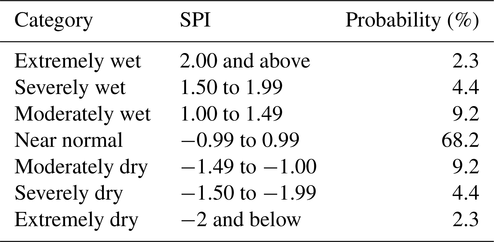
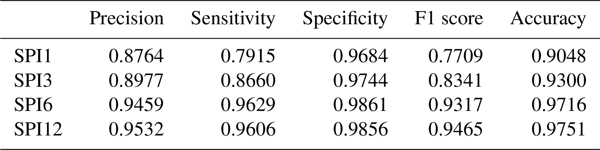
The mean SPI value is therefore zero. Negative values indicate dry anomalies, while positive values indicate wet anomalies. Table 3 reports drought classification according to the SPI. Conventionally, drought starts when SPI is lower than −1. The drought event is ongoing until SPI is up to 0 (McKee et al., 1993). The main strengths of the SPI are the fact that the index is standardised, and therefore can be used to compare different climate regimes, and that it can be computed for various accumulation periods (World Meteorological Organization and Global Water Partnership, 2016). In this study, SPI1, SPI3, SPI6 and SPI12 were computed, where the numeric values in the acronym refer to the period of accumulation in months (e.g. SPI3 indicates the standard precipitation index computed over a 3-month accumulation period). Shorter accumulation periods (1–3 months) are used to detect impacts on soil moisture and on agriculture. Medium accumulation periods (3–6 months) are preferred to identify reduced streamflow, and longer accumulation periods (12–48 months) indicate reduced reservoir levels (European Drought Observatory, 2020).
2.3 Machine learning algorithms
We now focus on the machine learning algorithms adopted in this work, starting with a short introduction and description of their basic functioning and next delving into the procedure used to build a large number of models based on the domain of possible configurations for each ML method. Finally, the metrics used to evaluate the models are introduced, and the reasoning behind their selection is highlighted.
2.3.1 Neural network (NN)
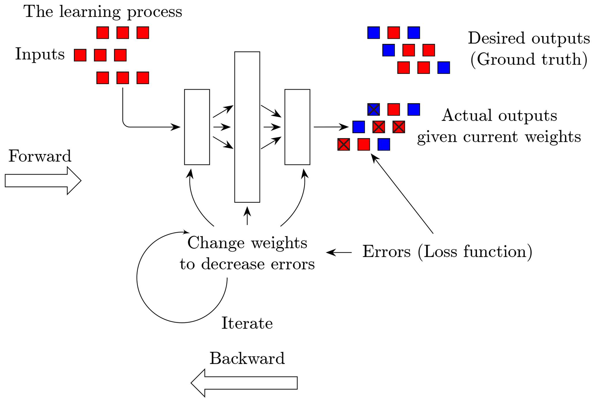
Neural networks are a machine learning algorithm composed by nodes (or neurons) that are typically organised into three types of layers: input, hidden and output. Once built, a neural network is used to understand and translate the underlying relationship between a set of input data (represented by the input layer) and the corresponding target (represented by the output layer). In recent years and with the advent of big data, neural networks have been increasingly used to efficiently solve many real-world problems, related for example with pattern recognition and classification of satellite images (Dreyfus, 2005), where the capacity of this algorithm to handle non-linearity can be put to fruition (Stevens and Antiga, 2019). A key problem when applying neural networks is defining the number of hidden layers and hidden nodes. This must usually be done specifically for each application case, as there is no globally agreed-on procedure to derive the ideal configuration of the network architecture (Mas and Flores, 2008). Although different terminology may be used to refer to neural networks depending on their architectures (e.g, artificial neural networks, deep neural networks), in this paper they are addressed simply as neural networks, specifying where needed the number of hidden layers and hidden nodes. Figure 2 displays the different parts composing a neural network and their interaction during the learning process. A neural network with multiple layers can be represented as a sequence of equations, where the output of a layer is the input of the following layer. Each equation is a linear transformation of the input data, multiplied by a weight (w) and the addition of a bias (b) to which a fixed non-linear function is applied (also called activation function):
The goal of these equations is to diminish the difference between the predicted output and the real output. This is attained by minimising a so-called loss function (LF) through the fine-tuning of the parameters of the model, the weights. The latter procedure is carried out by an optimiser, whose job is to update the weights of the network based on the error returned by the LF.
The iterative learning process can be summarised by the following steps:
-
start the network with random weights and bias;
-
pass the input data and obtain a prediction;
-
compare the prediction with the real output and compute the LF, which is the function that the learning process is trying to minimise;
-
backpropagate the error, updating each parameter through an optimiser according to the LF;
-
iterate the previous step until the model is trained properly – this is achieved by stopping the training process either when the LF is not decreasing anymore or when a monitored metric has stopped improving over a set amount of definition.
Specific to the training process, monitoring the training history can provide useful information, as this graphic representation of the process depicts the evolution over time of the LF for both training and validation set. Looking at the history of the training has a twofold purpose: firstly, with the training being a minimisation problem, as long as the LF is decreasing the model is still learning, while any eventual plateau or uprising would mean that the model is overfitting (or not learning anymore from the data). The latter is avoided when the LF of the training and validation dataset displays the same decreasing trend (Stevens and Antiga, 2019). The monitoring assignment is carried out during the training of the model, where its capability to store the value of training and validation loss at each iteration of the process enable the possibility to stop the training as soon as losses are either decreasing or plateauing over a certain number of iterations. In this work, the neural network model is created and trained using TensorFlow (Abadi et al., 2016). TensorFlow is an open-source machine learning library that was chosen for this work due to its flexibility, the capacity to exploit GPU cards to ease computational costs, its ability to represent a variety of algorithms and most importantly the possibility to carefully evaluate the training of the model.
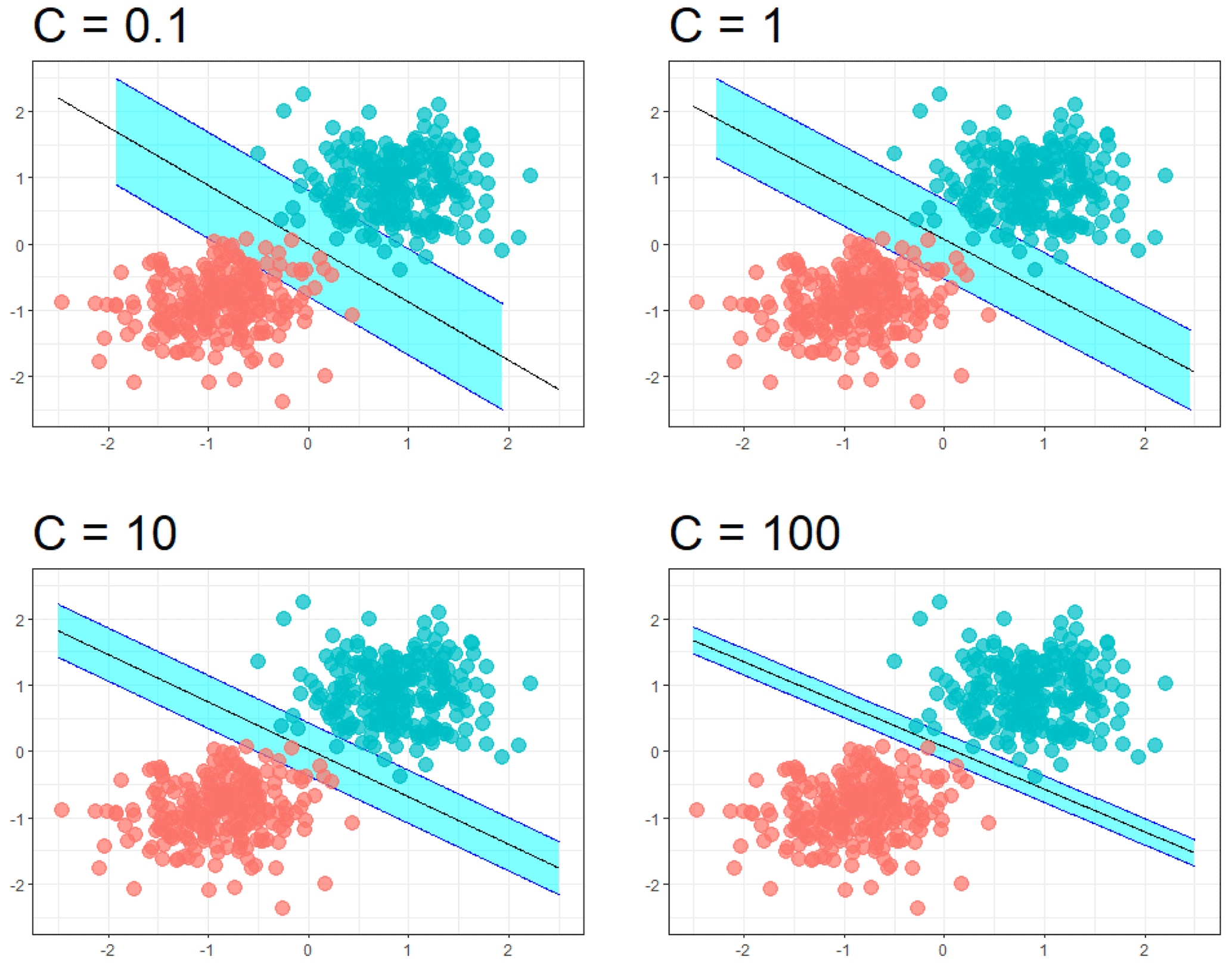
Figure 3Decision boundary of the support vector machine's algorithm, with changing regularisation parameter C.
2.3.2 Support vector machine (SVM)
The support vector machine is a supervised learning algorithm used mainly for classification analysis. It construct a hyperplane (or set of hyperplanes) defining a decision boundary between various data points representing observations in a multidimensional space. The aim is to create a hyperplane that separates the data on either side as homogeneously as possible. Among all possible hyperplanes, the one that creates the greatest separation between classes is selected. The support vectors are the points from each class that are the closest to the hyperplane (Wang, 2005). In parametric trigger modelling, as in many other real-world applications, the relationships between variables are non-linear. A key feature of this technique is its ability to efficiently map the observations into a higher-dimension space by using the so-called kernel trick. As a result, a non-linear relationship may be transformed into a linear one. A support vector machine can also be used to produce probabilistic predictions. This is achieved by using an appropriate method such as Platt scaling (Platt, 1999), which transforms its output into a probability distribution over classes by fitting a logistic regression model to a classifier's scores. In this work, the support vector machine algorithm was implemented using the C-support vector classification (Boser et al., 1992) formulation implemented with the scikit-learn package in Python (Pedregosa et al., 2011). Given training vectors and a label vector , this specific formulation is aimed at solving the following optimisation problem:
where ω and b are adjustable parameters of the function generating the decision boundary, Ψi is a function that projects xi into a higher dimensional space, ξi is the slack variable and C>0 is a regularisation parameter, which regulates the margin of the decision boundary, allowing an increasing number of misclassifications for a lower value of C and a decreasing number of misclassifications for higher C (Fig. 3).
2.3.3 Model construction
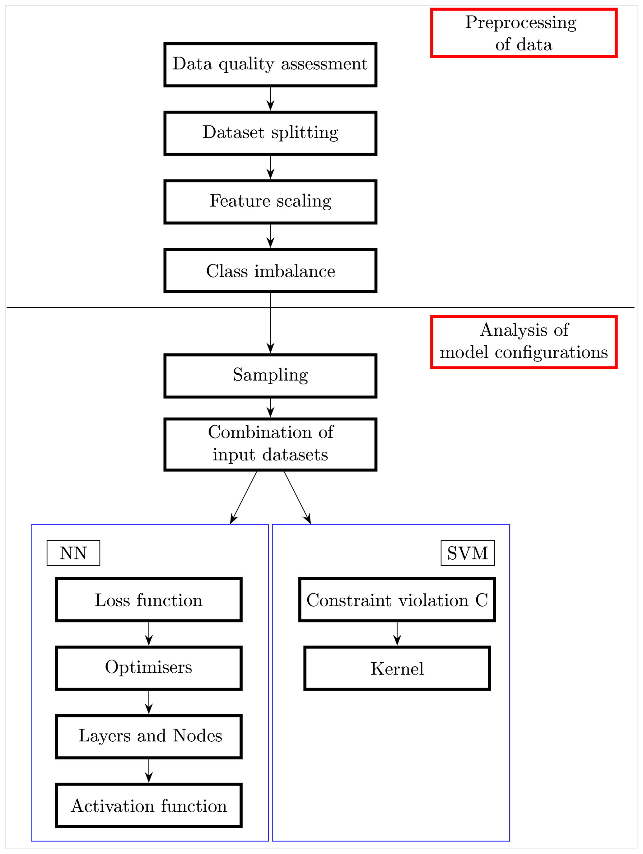
Below a procedure to assemble the machine learning models is proposed, which involves techniques borrowed from the data mining field and a deep understanding of all the components of the algorithms. The main purpose is to identify the actions required to establish a robust chain of model construction. Hypothetically speaking, one may create a neural network with an infinite number of layers or a support vector machine model with infinite values of the C regularisation parameters. Figure 4, an expanded diagram of the ML algorithm box of the workflow shown in Fig. 1, describes the steps followed in order to create the best-performing NN and SVM models from the focus placed on the importance of data enhancing to the selection of appropriate evaluation metrics, exploring as many model configuration as possible, being aware of the several parameters comprising these models and the wide ranges that these parameters can have.
Preprocessing of data
Data preprocessing (DPP) is a vital step to any ML undertaking, as the application of techniques aimed at improving the quality of the data before training leads to improvement of the accuracy of the models (Crone et al., 2006). Moreover, data preprocessing usually results in smaller and more reliable datasets, boosting the efficiency of the ML algorithm (Zhang et al., 2003). The literature presents several operations that can be adopted to transform the data depending on the type of task the model is required to carry out (Huang et al., 2015; Felix and Lee, 2019). In this paper, preprocessing operations were split into four categories: data quality assessment, data partitioning, feature scaling and resampling techniques aimed at dealing with class imbalance. The first three are crucial for the development of a valid model, while the latter is required when dealing with the classification of rare events. Data quality assessment was carried out to ensure the validity of the input data, filtering out any anomalous value (e.g. negative values of rainfall).
The partitioning of the dataset into training, validation and testing portions is fundamental to give the model the ability to learn from the data and avoid a problem often encountered in ML application: overfitting. This phenomenon takes place when a model starts overlearning from the training dataset, picking up patterns that belong solely to the specific set of data it is training on and that are not depictive of the real-world application at hand, making the model unable to generalise to sample outside this specific set of data. To avoid overfitting one should split the data into at least two parts (McClure, 2017): the training set, upon which the model will learn, and a validation dataset functioning as a counterpart during the training process of the model, where the losses obtained from the training set and those obtained from the validation set are compared to avoid overfitting. A further step would be to set aside a testing set of data that the model has never seen. Evaluating the performances of the model using data that it has never encountered before is an excellent indicator of its ability to generalise. Thus, the splitting of the data is key to the validation of the model. In this work, the training of the NN was carried out splitting the dataset into three parts: training (60 %), validation (15 %) and testing (25 %) sets. During training, the neural networks used only the training set, evaluating the loss on the validation set at each iteration of the training process. After the training, the performance of the model was evaluated on the testing set that the model has never seen. Concerning the SVMs, a k-fold cross validation (Mosteller and Tukey, 1968) was used to validate the model, using 5 folds created by preserving the percentage of sample of each class; the algorithm was therefore trained on 80 % of the data and its performances were evaluated on 20 % of the remaining data that the model had never seen.
Feature scaling is a procedure aimed at improving the quality of the data by scaling and normalising numeric values so as to help the ML model in handling varying data in magnitude or unit (Aksoy and Haralick, 2001). The variables are usually rescaled to the [0,1] range or to the range or normalised subtracting the mean and dividing by the standard deviation. The scaling is carried on after the splitting of the data and is usually calibrated over the training data, and then the testing set is scaled with the mean and variance of the training variables (Massaron and Muller, 2016).
Lastly, when undertaking a classification task, particular attention should be paid to addressing class imbalance, which reflects an unequal distribution of classes within a dataset. Imbalance means that the number of data points available for different classes is significantly different; if there are two classes, a balanced dataset would have approximately 50 % points for each of the classes. For most machine learning techniques, a little imbalance is not a problem, but when the class imbalance is high, e.g. 85 % points for one class and 15 % for the other, standard optimisation criteria or performance measures may not be as effective as expected (Garcia et al., 2012). Extreme events are by definition rare; hence, the imbalance existing in the dataset should be addressed. One approach to address imbalances is using resampling techniques such as oversampling (Ling and Li, 1998) and SMOTE (Chawla et al., 2002). Oversampling is the process of up-sampling the minority class by randomly duplicating its elements. SMOTE (Synthetic Minority Oversampling Technique) involves the synthetic generation of data looking at the feature space for the minority class data points and considering its k nearest neighbour where k is the desired number of synthetic generated data. Another possible approach to address imbalances is weight balancing, which restores balance in the data by altering the way the model “looks” at the under-represented class. Oversampling, SMOTE and class weight balancing were the resampling techniques deemed more appropriate to the scope of this work, namely, identifying events in the minority class.
Analysis of model configurations
Up to this point, several models characteristics and a considerable amount of possible operations aimed at data augmentation were presented, creating an almost boundless domain of model configurations. In order to explore such a domain, for each ML method multiple key aspects were tested. Both methods shared an initial investigation of the sampling technique and the combination of input datasets to be fed into the models; all the data resampling techniques previously introduced were tested along with the data in their pristine condition where the model tries to overcome the class imbalance by itself. All the possible combinations of input dataset were tested starting from one dataset for SVM and with two datasets for NN up to the maximum number of environmental variables used. The latter procedure can be used to determine whether the addition of new information is beneficial to the predictive skill of the model and also to identify which datasets provide the most relevant information.
As previously discussed, these models present a multitude of customisable facets and parameters. For the support vector machine, the regularisation parameter C and the kernel type were the elements chosen as the changing parts of the algorithm. Five different values of C were adopted, starting from a soft margin of the decision boundary moving towards narrower margins, while three kinds of kernel functions were used to find the separating hyperplane: linear, polynomial and radial. The setup for a neural network is more complex and requires the involvement of more parameters, namely, the LF and the optimisers concerning the training process, plus the number of layers and nodes and the activation functions as key building blocks of the model architecture. Each of the aforementioned parameters can be chosen among a wide range of options; moreover, there is not a clear indication for the number of hidden layers or hidden nodes that should be used for a given problem. Thus, for the purpose of this study, the intention was to start from what was deemed the “standard” for the classification task for each of these parameters, deviating from these standard criteria towards more niche instances of the parameters trying to cover as much as possible of the entire domain.
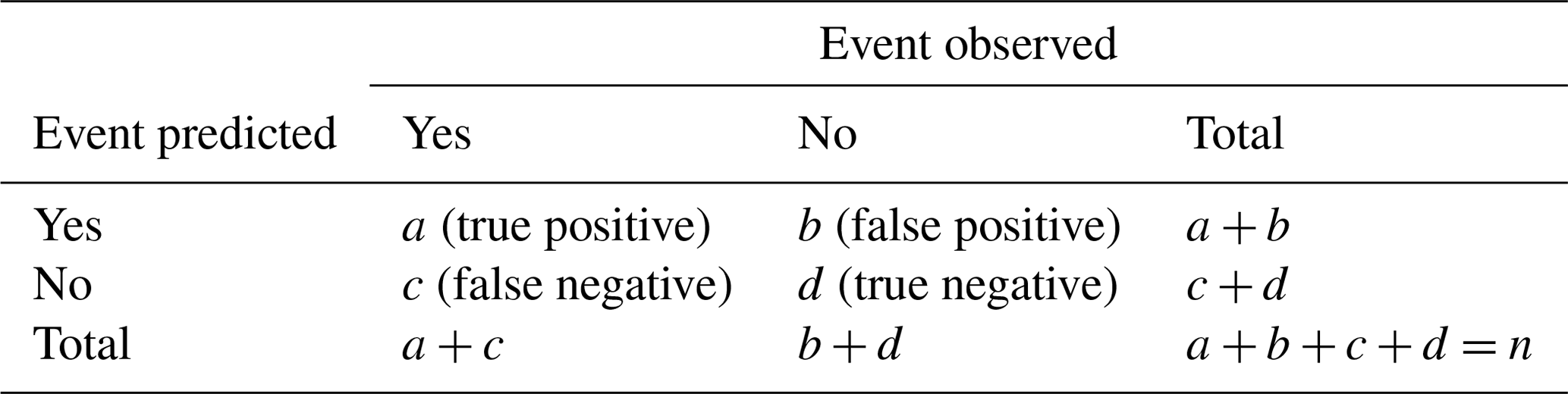
Table 4Contingency table for the deterministic estimates of a series of binary events.
2.4 Evaluation of predictive performance
The evaluation of the predictive performance of the models is fundamental to select the best configuration within the entire realm of possible configurations. A reliable tool to objectively measure the differences between model outputs and observations is the confusion matrix. Table 4 shows a schematic confusion matrix for a binary classification case. When dealing with thousands of configurations and, for each configuration, with an associated range of possible threshold probabilities, it is impracticable to manually check a table or a graph for each setup of the model. Therefore, a numeric value, also called evaluation metric, is often employed to synthesise the information provided by the confusion matrix and describe the capability of a model (Hossin and Sulaiman, 2015).
There are basic measures that are obtained from the predictions of the model for a single threshold value (i.e. value above which an event is considered to occur). These include the precision, sensitivity, specificity and false alarm rate, which take into consideration only one row or column of the confusion matrix, thus overlooking other elements of the matrix (e.g. high precision may be achieved by a model that is predicting a high value of false negatives). Nonetheless, they are staples in the evaluation of binary classification, providing insightful information depending on the problem addressed. Accuracy and F1 score, on the other hand, are obtained by considering both directions of the confusion matrix, thus giving a score that incorporates both correct predictions and misclassifications. The accuracy is the ratio between the correct prediction over all the instances of the dataset and is able to tell how often, overall, a model is correct. The F1 score is the harmonic mean of precision and recall. In its general formulation derived from the effectiveness measure of Jones and Van Rijsbergen (1976), one may define a Fβ score for any positive real β (Eq. 15):
where β denotes the importance assigned to precision and sensitivity. In the F1 score both are considered to have the same weight. For values of β higher than 1 more significance is given to false negatives, while β lower than 1 puts attention on the false positive.
Table 5Key metrics for the evaluation of model performance; a, b, c and d are defined in Table 4.

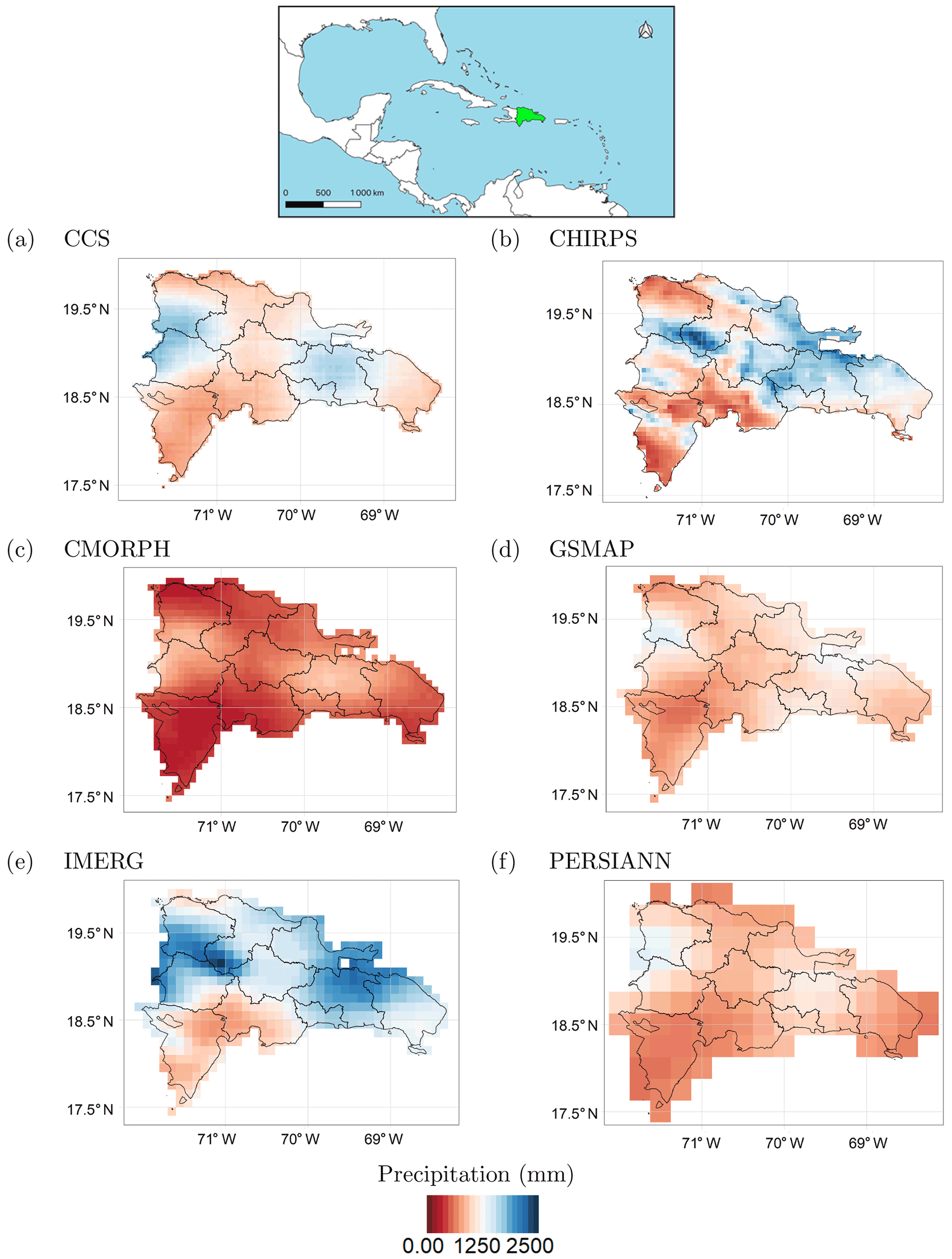
Figure 5Average annual rainfall over the Dominican Republic according to the six considered datasets. (a) CCS, (b) CHIRPS, (c) CMORPH, (d) IMERG, (e) GSMaP and (f) PERSIANN.
The goodness of a model may also be assessed in broader terms with the aid of receiver operating characteristic (ROC) and precision-sensitivity curves (PS). The ROC curve is widely employed and is obtained by plotting the sensitivity against the false alarm rate over the range of possible trigger thresholds (Krzanowski and Hand, 2009). The PS curve, as the name suggests, is obtained by plotting the precision against the sensitivity over the range of possible thresholds. For this work, the threshold corresponds to the range of probabilities between 0 and 1. These methods allow for evaluating a model in terms of its overall performance over the range of probabilities, by calculating the so-called area under the curve (AUC). It should be noted that both the ROC curve and the accuracy metric should be used with caution when class imbalance is involved (Saito and Rehmsmeier, 2015), as having a large amount of true negative tends to result in a low false-positive-rate value (FPR ). Table 5 summarises the metrics described above used in this paper to evaluate model performances.
In the context of performance evaluation, it is also relevant to discuss how class imbalance might affect measures that use the true negative in their computation. Saito and Rehmsmeier (2015) tested several metrics on datasets with varying class imbalance and showed how accuracy, sensitivity and specificity are insensitive to the class imbalance. This kind of behaviour from a metric can be dangerous and definitely misleading when assessing the performances of a ML algorithm and might lead to the selection of a poorly designed model (Sun et al., 2009), emphasising the importance of using multiple metrics when analysing model performances. Lastly, once the domain of all configurations was established and the best settings of the ML algorithms were selected based on the highest values of F1 score and area under the PS curve, the predictive performances of the models were compared to those of logistic regression (LR) models. The logistic regression adopted as a baseline takes as input multiple environmental variables, in line with the procedure followed for the ML methods, and used a logit function (Eq. 6) as a link function, neglecting interaction and non-linear effects amid predictors. The logistic regression is a more traditional statistical model whose application to index insurance has recently been proposed and can be said to already represent in itself an improvement over common practice in the field (Calvet et al., 2017; Figueiredo et al., 2018). Thus, this comparison is able to provide an idea about the overall advantages of using a ML method.
This study adopts the Dominican Republic as its case study. The Dominican Republic is located on the eastern part of the island of Hispaniola, one of the Greater Antilles, in the Caribbean region. Its area is approximatively 48 671 km2. The central and western parts of the county are mountainous, while extensive lowlands dominate the south-east (Izzo et al., 2010).
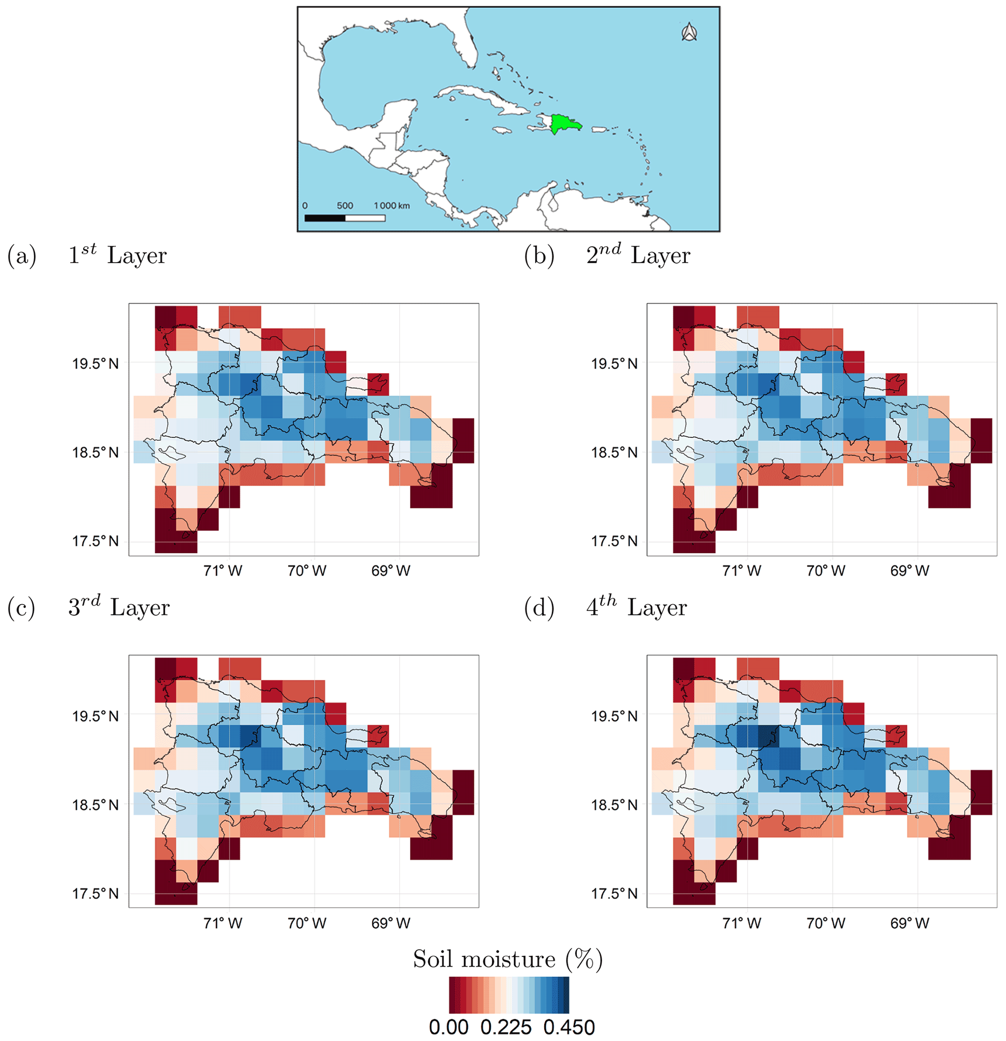
Figure 6Average soil moisture over the Dominican Republic in the four soil moisture layers. (a) First layer, 0–7 cm; (b) second layer, 7–28 cm; (c) third layer, 28–100 cm; (d) fourth layer, 100–289 cm.
The climate of the Dominican Republic is classified as “tropical rainforest”. However, due to its topography, the country's climate shows considerable variations over short distances. The average annual temperature is about 25 ∘C, with January being the coldest month (average monthly temperature over the period 1901–2009 of about 22 ∘C) and August the hottest (average monthly temperature over the period 1901–2009 of about 26 ∘C) (World Bank, 2019). Rainfall varies from 700 to 2400 mm yr−1, depending on the region (Payano-Almanzar and Rodriguez, 2018). The six considered rainfall datasets (described in Table 1) exhibit considerable differences in average annual precipitation values over the Dominican Republic (Fig. 5), with CMORPH showing the lowest values and CHIRPS and IMERG the highest ones. Nevertheless, the difference among absolute precipitation values does not affect the results of this study since precipitation is transformed into potential damage or SPI, as described in Sect. 2.2.2, and therefore only relative values are considered. It is interesting to note that all the datasets show similar precipitation patterns; on average, over the period from 2000 to 2019, rainfall was mainly concentrated in north-western regions, along the Haitian borders, with the south-western regions being the driest. The situation is different when considering the average soil moisture (Fig. 6). The central regions are the wettest, while the driest areas are located on the coast. There are no significant differences among the four soil moisture layers.
Weather-related disasters have a significant impact on the economy of the Dominican Republic. The country is ranked as the 10th most vulnerable in the world and the second in the Caribbean, as per the Climate Risk Index for 1997–2016 report (Eckstein et al., 2017). It has been affected by spatial and temporal changes in precipitation, sea level rise, and increased intensity and frequency of extreme weather events. Climate events such as droughts and floods have had significant impacts on all the sectors of the country's economy, resulting in socio-economic consequences and food insecurity for the country. According to the International Disaster Database EMDAT (CRED, 2019), over the period from 1960 to present, the most frequent natural disasters were tropical cyclones (45 % of the total natural disasters that hit the country), followed by floods (37 %) . Floods, storms and droughts were the disasters that affected the largest number of people and caused huge economic losses.

Figure 7Overview of floods and droughts hitting the Dominican Republic over the period 2000–2019.
The performances of a ML model are strictly related to the data the algorithm is trained on; hence, the reconstruction of historical events (i.e. the targets), although time-consuming, is paramount to achieve solid results. Therefore, a wide range of text-based documents from multiple sources have been consulted to retrieve information on past floods and droughts that hit the Dominican Republic over the period from 2000 to 2019. International disasters databases, such as the world-renowned EMDAT, Desinventar and ReliefWeb, have been considered as primary sources. The events reported by the datasets have been compared with the ones present in hazard-specific datasets (such as FloodList and the Dartmouth Flood Observatory) and in specific literature (Payano-Almanzar and Rodriguez, 2018; Herrera and Ault, 2017) to produce a reliable catalogue of historical events. Only events reported by more than one source were included in the catalogue. Figure 7 shows the past floods and droughts hitting the Dominican Republic over the period from 2000 to 2019. More details on the events can be found in Tables A1 (floods) and A2 (droughts).
Table 6Breakdown of all the configuration explored by algorithm and type of hazard.
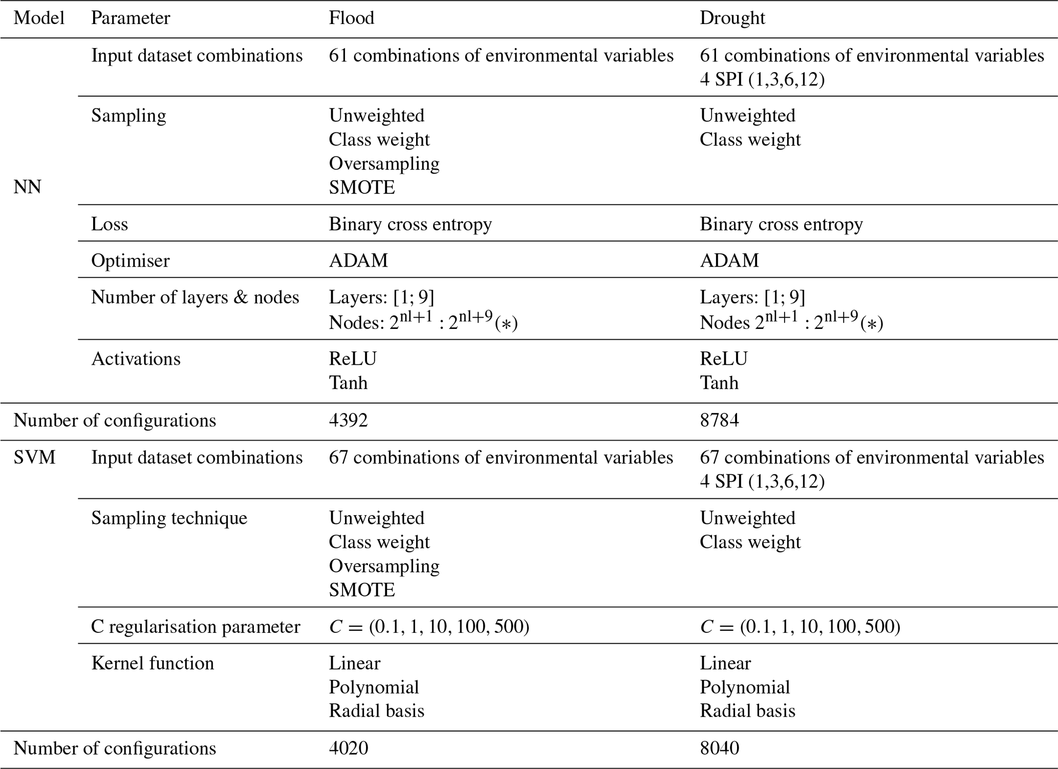
* nl: number of layers.
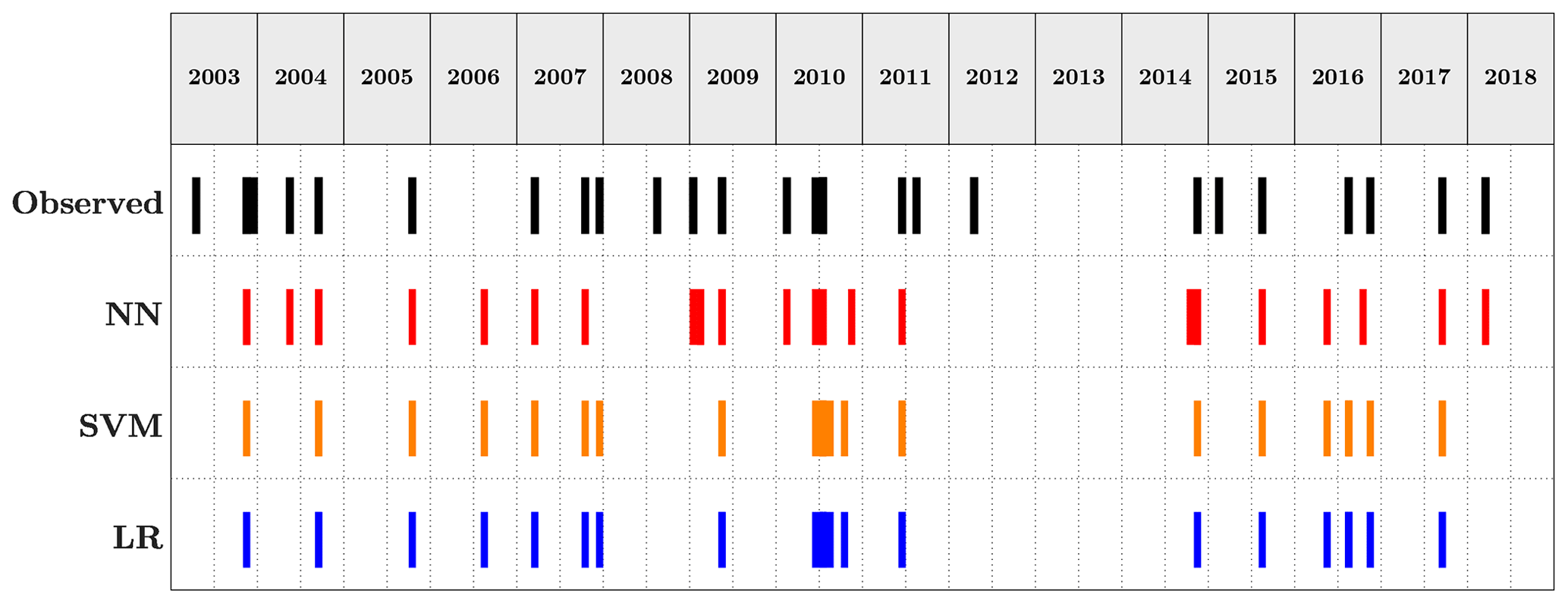
Figure 8Comparison of the predictions of the three methods over the testing set vs. the observed events. Flood case.
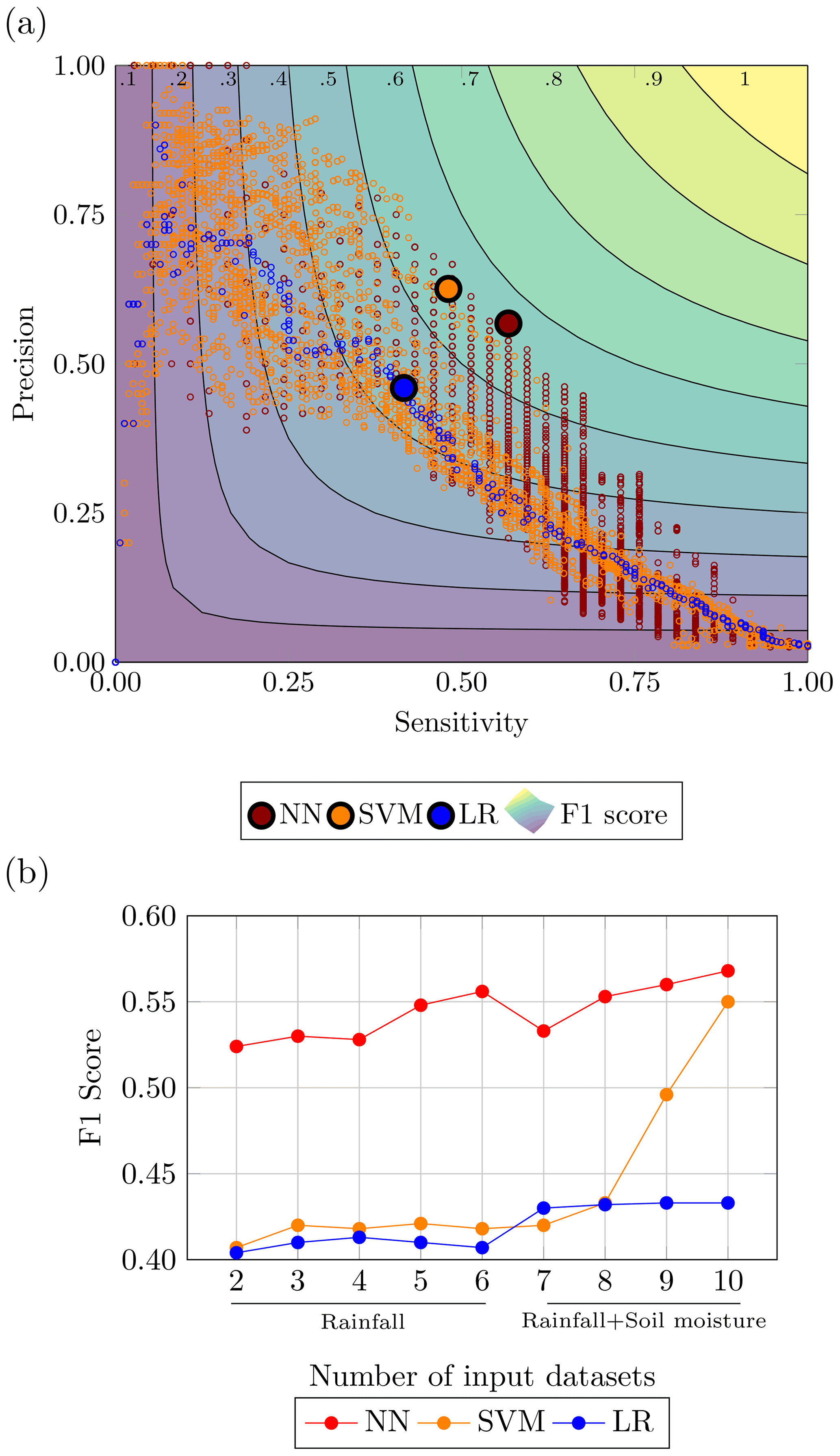
Figure 9Performance evaluation for the flood case: (a) performances of the top 1 % configurations in the precision-sensitivity space highlighting the highest F1 score and (b) comparison of ML methods with LR with combination using increasing number of input datasets.
The results are presented in this section separating the two types of extreme events investigated, flood and drought. As described in Sect. 2, both NN and SVM models require the assembling of several components. Table 6 collects the number of model configurations explored, broken down by type of hazard and ML algorithm with their respective parameters. The main differences between the ML models parameters for the two hazards reside in which data are provided to the algorithm and which sampling techniques are adopted. The input dataset combination were chosen as follows:
-
all the possible combinations from one up to six rainfall datasets (for neural networks two rainfall datasets were considered the starting point);
-
the remaining combinations are obtained adding progressively layers of soil moisture to the ensemble of six rainfall datasets;
-
the drought case required the investigation of the SPI over different accumulation periods, and 1-, 3-, 6- and 12-month SPI values were used.
Neural networks and support vector machines alike are able to return predictions (i.e. outputs) as a probability when the activation function allows it (e.g. sigmoid function), enabling the possibility to find an optimal value of probability to assess the quality of the predictions . Therefore, for each hazard, the results are presented by introducing at first the models achieving the highest value of the F1 score for a given configuration and threshold probability (i.e. a point in the ROC or precision-sensitivity space). Secondly, the best-performing model configurations for the whole range of probabilities according to the AUC of the precision-sensitivity curve are presented and discussed. The reasoning behind the selection of these metrics is discussed in Sect. 2.4. As described in the same section, the performances of the ML algorithms are evaluated through a comparison with a LR model.
Table 7Comparison metrics best configuration for flood by method.
4.1 Flooding
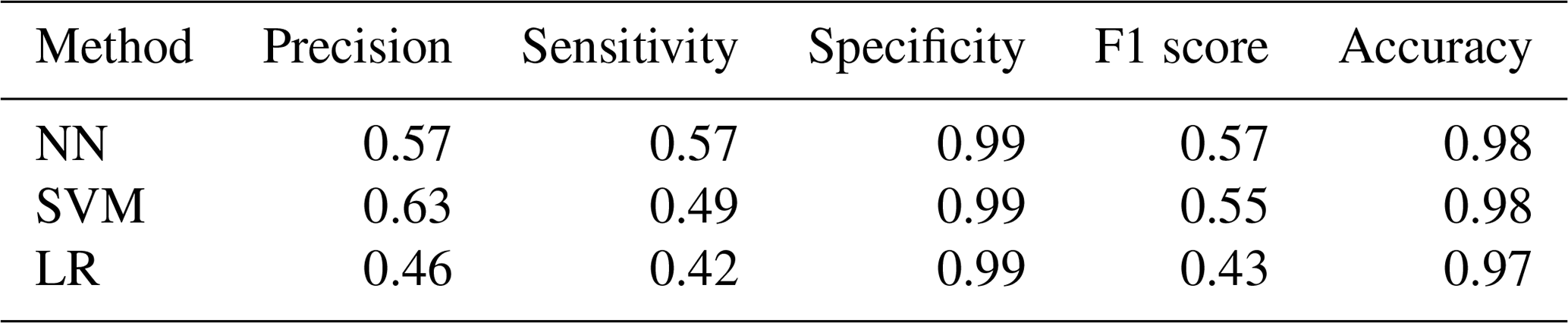
The flood case presented a strong challenge from the data point of view. Inspecting the historical catalogue of events the case study reported 5516 d with no flood events occurring and 156 d of flood, meaning approximately a 35:1 ratio of no event event. This strong imbalance required the use of the data augmentation techniques presented in Sect. 2.3.1. The neural network settings returning the highest F1 score were given by the model using all 10 datasets applying an oversampling to the input data. The network architecture was made up of nine hidden layers with the number of nodes for each layer as already described, activated by a ReLU function. The LF adopted was the binary cross entropy, and the weights update was regulated by an Adam optimiser. The highest F1 score for the support vector machine was attained by the model configuration using an unweighted model taking advantage of all 10 environmental variables with a radial basis function as kernel type and a C parameter equal to 500 (i.e. harder margin). Figure 8 shows the predictions of the two machine learning models and the baseline logistic regression, as well as the observed events. The corresponding evaluation metrics are summarised in Table 7, which refer to results measured on the testing set and, therefore, never seen by the model. Overall, the two ML methods outperform decisively the logistic regression with a slightly higher F1 score for the neural network.
In Fig. 9a the highest F1 scores by method are reported in the precision-sensitivity space along with all the points belonging to the top 1 % configurations according to F1 score. The separation between the ML methods and the logistic regression can be appreciated, particularly when looking at the emboldened dots in Fig. 9 representing the highest F1 score for each method. Also, the plot highlights a denser cloud of orange points in the upper left corner and a denser cloud of red points in the lower right corner, attesting, on average, a higher sensitivity achieved by the NNs and a higher precision by the SVMs.
Figure 9b depicts the goodness of NN and SVM vs. the LR model, showing how the F1 scores of the best-performing settings for each of the three methods vary by increasing the number of input datasets. This plot shows that the SVM and LR models have similar performances up to the second layer of soil moisture, while NN performs considerably better overall. The NN and the SVM as opposed to the LR show an increase in the performances of the models with increasing information provided. The LR seems to plateau after four rainfall datasets, and the improvements are minimal after the first layer of soil moisture is fed to the model. This would suggest, as expected, that the ML algorithms are better equipped to treat larger amounts of data.
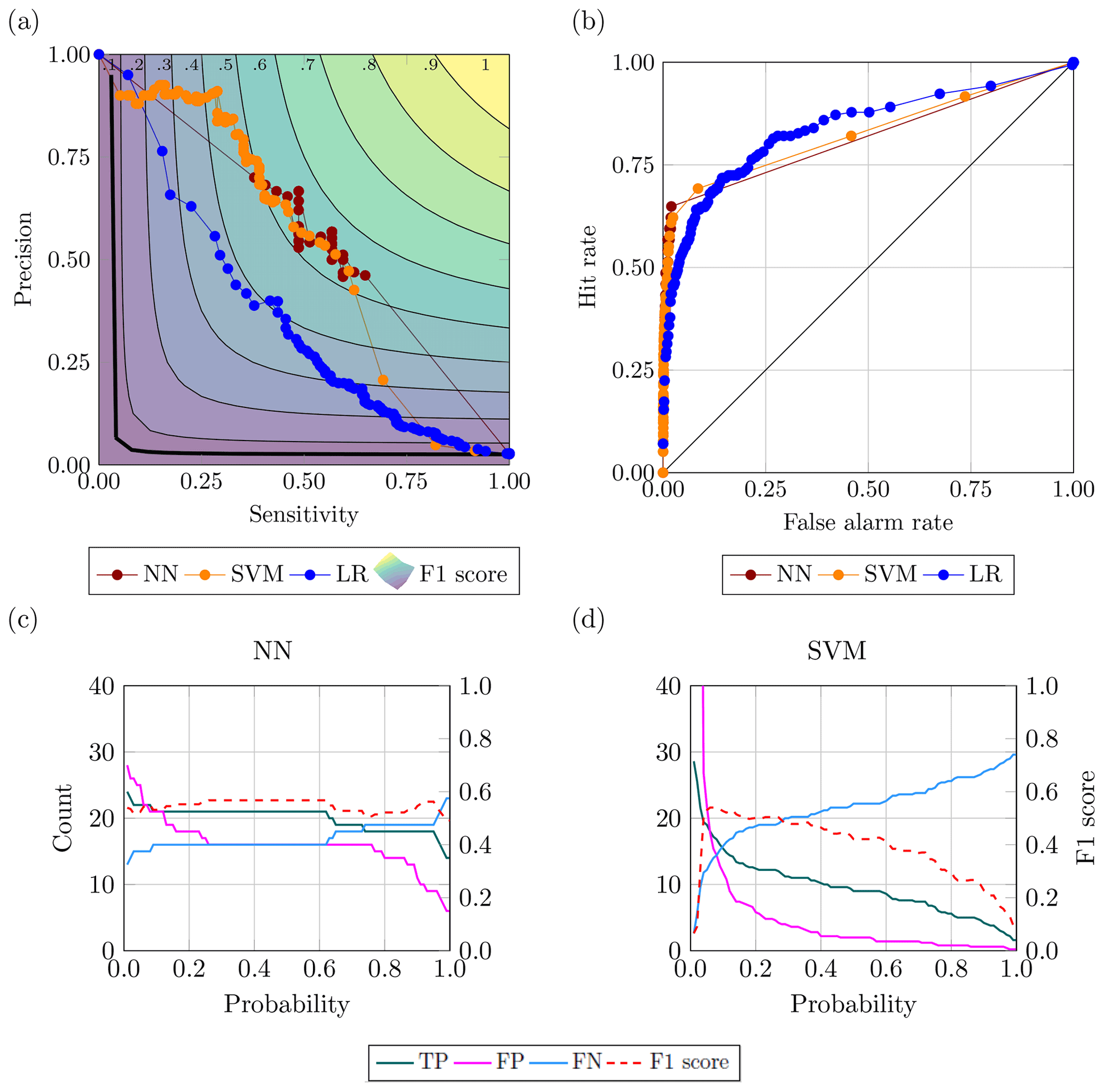
Figure 10Best-performing configurations for the flood case: (a) PS curve; (b) ROC curve; and variation of true positive, false positive, true negative and F1 score for the range of probability (c) in NN and (d) in SVM.
Figure 10 presents the best-performing configurations according to the area under the PS curve. For neural network, this configuration is the one that also contains the highest F1 score, whereas for support vector machine the optimal configuration shares the same feature of the one with the best F1 score with the exception of a softer decision boundary in the form of C equal to 100. The results reported in Fig. 10a and b about the best-performing configurations are further confirmation of the importance of picking the right compound measurement to evaluate the predictive skill of a model. In fact, according to the metrics using the true negative in their computation (i.e. specificity, accuracy and ROC), one may think that these models are rather good, and this deceitful behaviour is not scaled appropriately for very bad models. The aim of this work is to correctly identify a flood event rather than being correct when none occur; hence, overlooking the correct rejections seems reasonable.
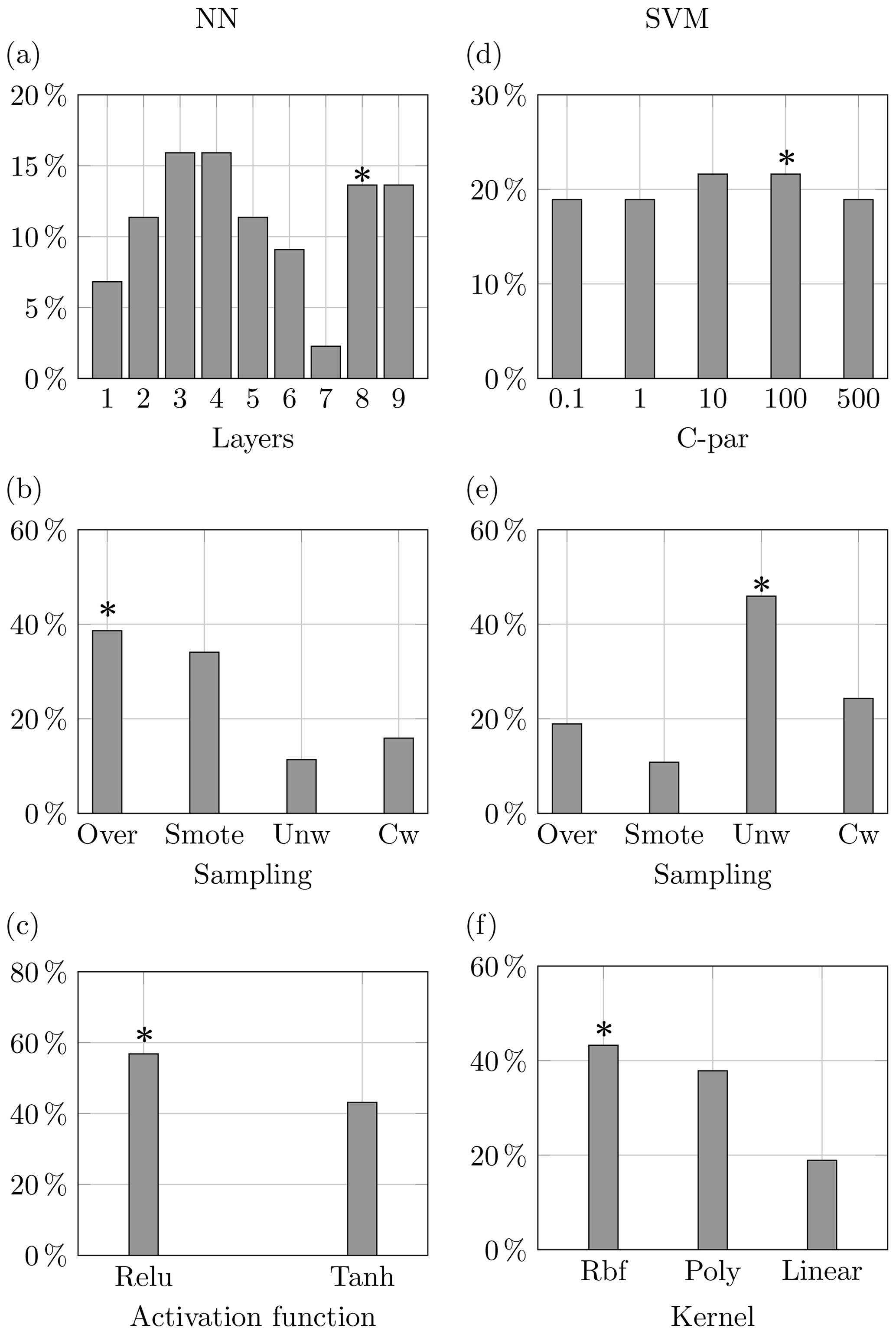
Figure 11Properties of top 1 % model configurations for the flood case. The stars denote the characteristics of the best-performing configurations according to the highest area under the precision-sensitivity curve.
Figure 10a and b shed a light on the inaccuracy of the ROC curve and the relative area under the curve (AUC). On the right the ROC curves are displayed, whilst on the left the PS curves of the ideal configurations for each method according to the highest AUC are displayed. The points in both curves represent a 0.01 increment in the trigger probability. The receiving operator curve indicates the NN as the worst model being the closest to the 45∘ line and having, along with SVM, a lower AUC with respect to the logistic model. This signal is strongly contradicted by other metrics and the precision-sensitivity curve, where the red dots are the closest to the upper-right corner where the perfect model resides. The behaviour of these curves is linked, once again, to the disparity in the classes. Additionally, looking at Fig. 10a, all models are pretty distant from the always-positive classifier (i.e. a baseline independent from class distribution represented by the black hyperbole in bold) more appropriate as a baseline to beat than a random classifier (Flach and Kull, 2015).
Figure 10c and d show the behaviour of the prediction return by the ML models over the whole range of probabilities. It is noticeable that although the peak value of the F1 score is very close for both ML methods, the neural network displays steadier prediction over an extended range of probabilities. In fact, a robust identification of the true positive and low variability in false-positive and false-negative detection allows the model to have strong performances independently of which probability threshold one may choose.
Table 8Comparison metrics best configuration for drought by method.
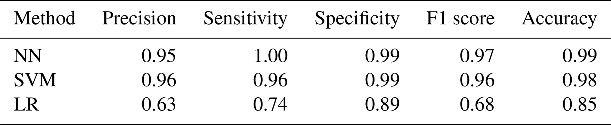
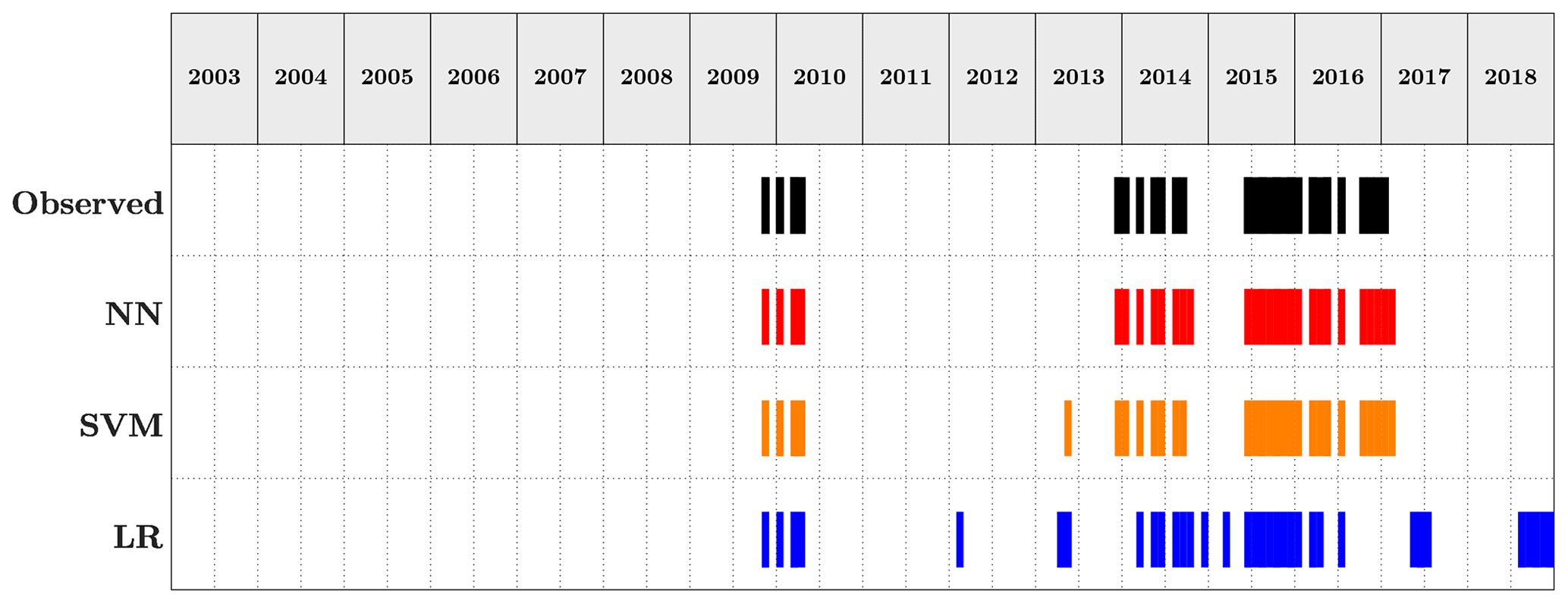
Figure 12Comparison of the predictions of the three methods over the testing set vs. the observed events. Drought case.
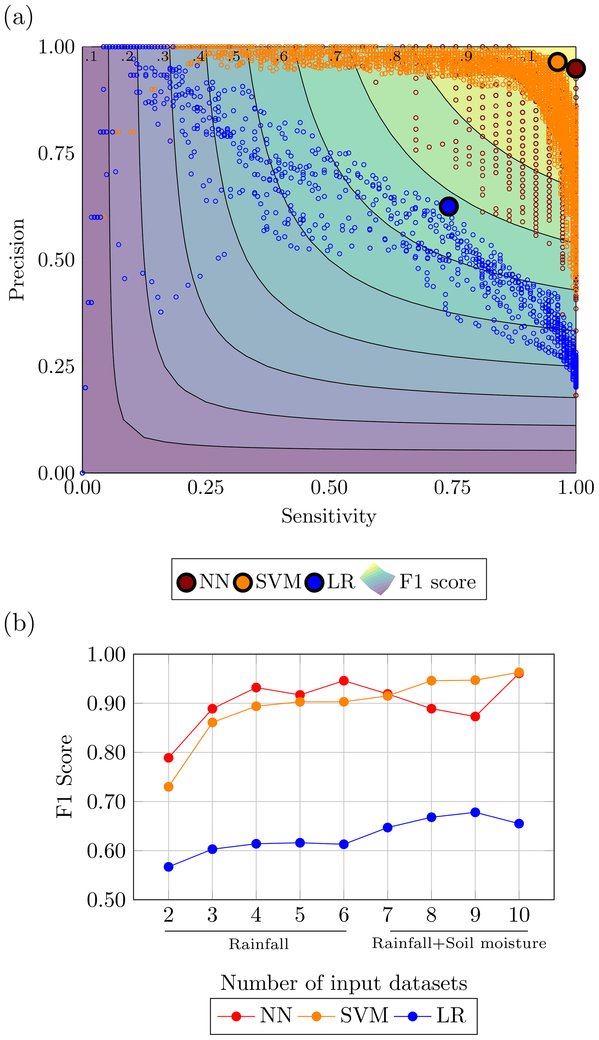
Figure 13Performance evaluation for the drought case: (a) performances of the top 1 % configurations in the precision-sensitivity space highlighting the highest F1 score and (b) comparison of ML methods with LR with combination using increasing number of input datasets.
Figure 11 portrays the properties of the top 1 % model configuration for both methods according to the area under the PS curve. Neural networks prefer the adoption of oversampling to enhance the input data, and almost 60 % of the configurations use a rectified linear unit function to activate its layer. Relative to the architecture of the network, a double peak can be observed at eight and nine layers, where the best-performing configurations can be found, but an even larger presence of model configuration with layers is noticeable. On the other hand, support vector machines use the highest value of the C parameter, which is the one used by the configuration attaining the highest F1 score. A bigger divide can be observed amid the sampling technique and the kernel function, where data input with no manipulation provided (i.e. unweighted) is the most recurrent option occurring more than 40 % of the time; a similar percentage is attained by the radial basis function.
4.2 Drought
The data transformation for drought required the computation of the SPI from the precipitation data. The SPI was computed for different accumulation periods: shorter accumulation periods (1–3 months) detect immediate impacts of drought (on soil moisture and on agriculture), while longer accumulation periods (12 months) indicate reduced streamflow and reservoir levels. As shown in tables B1 and B2 models using SPI6 and SPI12 showed the best results, and the values of the metrics are close to each other; thus, for brevity and in favour of clarity only one of the two is reported, namely, SPI over a 6-month accumulation period. Contrary to the flood case, the drought historical catalogue of events reported 1283 weeks with no droughts and 696 weeks of drought, with a ratio around 1.85:1 of no event event. Albeit balanced, models with weights assigned were also investigated. The performances of the neural networks and the support vector machines were evaluated, like before, by a set of evaluation metrics and curves and a comparison against a logistic regression. It is important to point out that SPI is updated at a weekly scale, with the same temporal resolution of the predictions, implying that each week counts as an event. Considering the duration of the drought in our historical catalogue of events (i.e. 17 weeks for the shortest one and 148 weeks for the longest), the temporal resolution adopted is an aspect to keep in mind when analysing the results obtained for these models. The highest F1 scores for the drought case were obtained for the NN model using all the datasets with weights for the classes. The network architecture was made up of eight hidden layers with the relative number of nodes activated by a ReLU function. The LF adopted was the binary cross entropy, and the parameter updates were regulated by an Adam optimiser. Regarding the SVM, the highest F1 score was achieved from the unweighted model using all 10 environmental variables with radial basis function as kernel type and a C parameter equal to 100.
Figure 12 displays the predictions of the three methods against the observed events. In particular, it is possible to appreciate the reduction of false positive provided by NN and SVM. The strong improvements brought by the ML algorithms are confirmed by the metrics summarised in Table 8, where NN and SVM show high values across all the prediction skill measurements. The NN results as the most accurate model, while the SVM is the more precise overall. The implementation of either model should take into account the job that these models are required to take on. If the purpose of the model is to balance the occurrences of false alarms and missed events, the NN is preferable. For a task that would require a stronger focus on the minimisation of false positives (i.e. reduce the number of false alarms), the SVM should be used. Figure 13 remarks the distance between the ML methods and the logistics regression as well as echoes what is observed for flood – that the points for NN gravitate towards the area of the plot with a higher sensitivity value, while the SVM points tend to stay on the precision side of the plot.
The addition of further datasets is still beneficial to the performances of the ML methods as displayed by Fig. 13b. The increasing trend for both ML models starts to slow down from the fourth rainfall datasets onward, which might be due to the redundancy of the rainfall datasets. On the other hand, the addition of the layers of soil moisture improves the performances especially for the support vector machine, which keeps improving steadily, reaching the highest value of F1 score when the whole set of information is fed to the model.
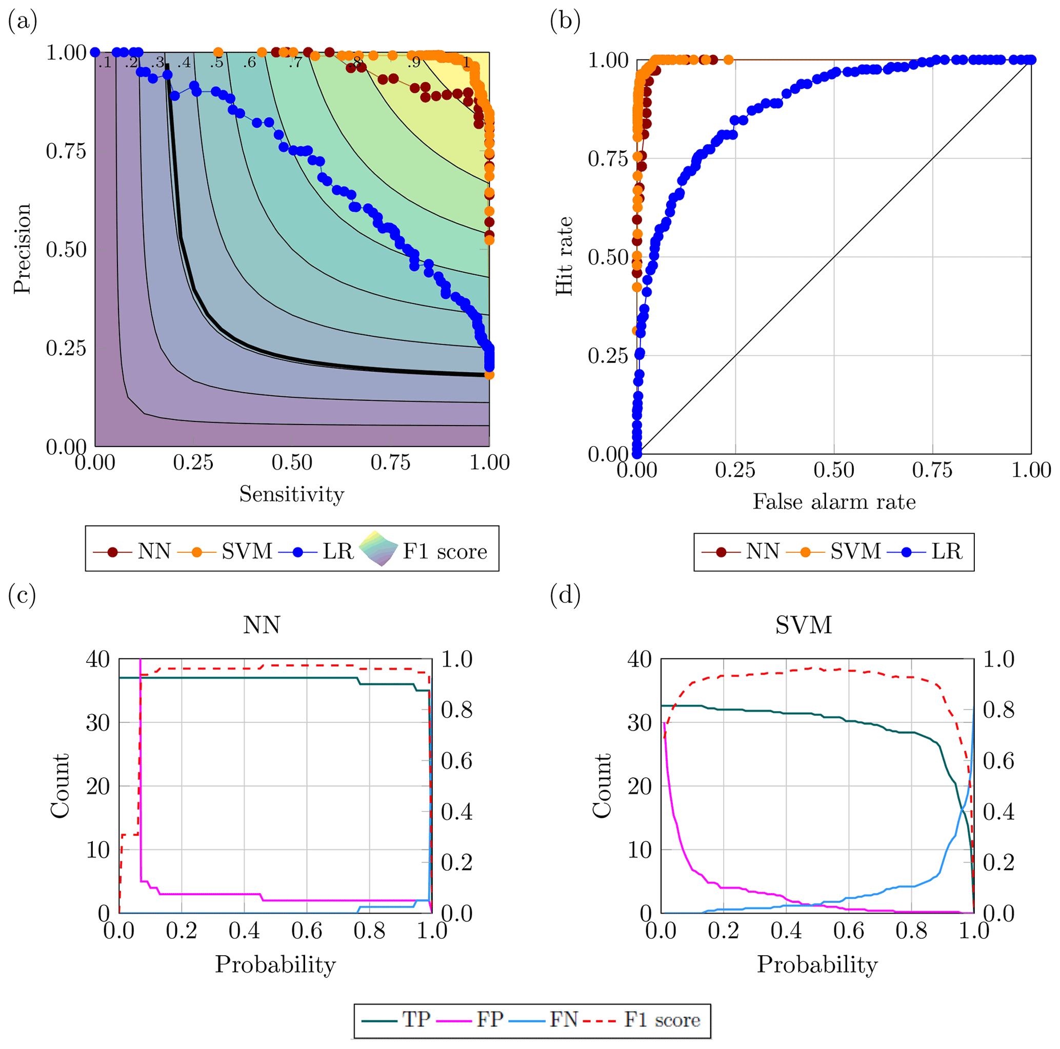
Figure 14Best-performing configurations for the drought case: (a) PS curve; (b) ROC curve; and variation of true positive, false positive, true negative and F1 score for the range of probability (c) in NN and (d) in SVM.

Figure 15Properties of top 1 % model configurations for the drought case. The stars denote the characteristics of the best-performing configurations according to the highest area under the precision-sensitivity curve.
Figure 14 refers to the best-performing configurations identified as the ones with the highest area under the precision-sensitivity curve. The best configurations for either neural network and support vector machine are the ones containing the point with the highest F1 score, thus having the same features previously listed. The disparities between classes for drought are closer than those for flood, giving the accuracy, and the ROC curve, more reliability from a quality assessment point of view. Looking at Fig. 14a and b, both precision-sensitivity and ROC curves show the ML methods decisively outperforming the no-skill and always-positive classifier. Furthermore, both plots exhibit a tendency of the neural network to group the points closer to each other towards the area containing the ideal model, which may indicate a more dependable prediction of the events as indicated by Fig. 14c. In fact, while the two configurations have a high value of F1 score for a wide range of probabilities, the neural network has steadier prediction of true positive, false positive and false negative. This behaviour of the neural network could also be linked to the miscalibration of the confidence (i.e. distance between the probability returned by the model and the ground truth) associated with the predicted probability (Guo et al., 2017). The phenomenon arose with the advent of modern neural networks that employ several layers (i.e. tens and hundreds) and a multitude of nodes were able to improve the accuracy of their prediction while worsening the confidence of said prediction. Indeed, a miscalibrated neural network would return a probability that would not reflect the likelihood that the event will occur, turning into a numeric output produced by the model.
The feature breakdown of the top 1 % model configurations shown in Fig. 15 shows that the best NN configurations are predominantly the ones using weight for the two classes and the ReLU activation function. Also, a large number of models use a high number of layers in accordance with the configuration with the highest area under the PS curve. The fact that most of the configurations obtaining the best performances have deeper layers may be a confirmation of the miscalibration affecting the estimated probabilities. For the SVM models, Fig. 15 denotes a marked component of the models using harder margins (i.e. high values of the C parameter) and the radial basis function as a kernel.
In this study we developed and implemented a machine learning framework with the aim of improving the identification of extreme events, particularly for parametric insurance. The framework merges a priori knowledge of the underlying physical processes of weather events with the ability of ML methods to efficiently exploit big data and can be used to support informed decision making regarding the selection of a model and the definition of a trigger threshold. Neural network and support vector machine models were used to classify flood and drought events for the Dominican Republic, using satellite data of environmental variables describing these two types of natural hazards. Model performance was assessed using state-of-the-art evaluation metrics. In this context, we also discussed the importance of using appropriate metrics to evaluate the performances of the models, especially when dealing with extreme events that may have a strong influence on some performance evaluators. It should be noted that while here we have focused on performance-based evaluation measures, an alternative approach would be to quantify the utility of the predictive systems. By taking into account actual user expenses and thus specific weights for different model outcomes, a utility-based approach could potentially lead to different decisions regarding model selection and definition of the trigger threshold (Murphy and Ehrendorfer, 1987; Figueiredo et al., 2018). This aspect is outside the scope of the present article and warrants further research.
The proposed approach involves a preceding data manipulation phase where the data are preprocessed to enhance the performances of the ML methods. A procedure aimed at designing and selecting the best parameters for the models was also introduced. Once trained, the ML algorithms decisively outperformed the logistic regression, here used as a baseline for both hazards. The predictive skill of both NN and SVM improved with increasing information fed to the models; indeed, the best performances were always obtained by models using the maximum number of data available, hinting at the possibility of introducing additional and more diverse environmental variables to further improve the results. While the ML models performed well for both hazards, the drought case showed exceptionally high values for all the adopted model evaluation metrics. This discrepancy in the results between flood and drought might have several explanations. Indeed, the two hazards behave differently both in time and space. On the one hand, the aggregation at a national scale is surely an obstacle for a rather local phenomenon like flood. On the other hand, defining a drought event weekly could be misleading since droughts are events spanning several months and even years. Using a higher resolution (e.g. regional scale) and introducing data describing the terrain of the area should enhance the detection of flood events. For the drought case, introducing a threshold for the number of consecutive weeks predicted before considering an event or contemplating weekly predictions as a fraction of the overall duration of the event are extensions to this work that deserve investigation to address the issue of potential overestimation of predictive skill.
Neural networks showed more robustness when compared to support vector machines, showing a higher value of F1 score for a wide range of parameters. As already mentioned, this insensitivity of NN to the probability threshold adopted may lead back to the inability of the model to reproduce probability estimates that are a fair representation of the likelihood of occurrence of the event. Further developments of neural networks models should take into consideration procedures that allow the assessment and the quantification of the confidence calibration of probability estimates.
A preliminary investigation of the characteristics shared by the best-performing model showed that some features are more relevant than others when building the ML model, depending on the type of algorithm and also the type of hazard. An in-depth study of how the performances of the models change when changing model properties could highlight which are the most important properties of the model to tune, speeding up the model construction phase and reducing the computational cost of running the algorithms. It is also worth noting that albeit this work focuses on the application of neural network and support vector machine models, we expect that comparable results could be obtained using other machine learning algorithms, which calls for further research.
Although several issues raised in this article warrant further research, there is clear potential in the application of machine learning algorithms in the context of weather index insurance. The first reason for this is strictly linked to the performances of the models. Indeed, the capability of these algorithms to reduce basis risk with respect to traditional methods could play a key role in the adoption of parametric insurance in the Dominican context and more generally for those countries that possess a low level of information about risk. The second aspect, perhaps the most intriguing from the weather index insurance point of view, regards the ability of these algorithms to utilise and improve their performances using a growing amount of information (i.e. increasing the number of input variables). Indeed, the significant advances in data collection and availability observed in the last decades (i.e. improved instruments, more satellite missions, open access to data store services) made it so that a vast number of data are readily and freely available on a daily basis. Being able to rely on global data that are disentangled from the resources of a given territory, both from the point of view of climate data (e.g. lack of rain-gauge networks) and from the point of view of information about past natural disasters, is an important feature of the work presented that would make the proposed approach feasible and appealing for other countries. Furthermore, similar technological improvements might be expected in the further development of machine learning algorithms. The scientific evolution of these models and the possibility of establishing a pipeline that automatically and objectively trains the algorithm over time with updated and improved data (always allowing the monitoring of the process) are other appealing features of these kinds of models. In conclusion, the framework presented and topics discussed in this study provide a scientific basis for the development of robust and operationalisable ML-based parametric risk transfer products.
The following tables report the catalogue of historical events for floods (Table A1) and droughts (Table A2).
ADRC and UNDRR (2020)CRED (2019)ADRC and UNDRR (2020)CRED (2019)Brakenridge (2002)Brakenridge (2002)ADRC and UNDRR (2020)CRED (2019)ADRC and UNDRR (2020)Brakenridge (2002)Brakenridge (2002)CRED (2019)OCHA (2020)Brakenridge (2002)CRED (2019)ADRC and UNDRR (2020)CRED (2019)ADRC and UNDRR (2020)CRED (2019)ADRC and UNDRR (2020)Brakenridge (2002)ADRC and UNDRR (2020)ADRC and UNDRR (2020)CRED (2019)Brakenridge (2002)ADRC and UNDRR (2020)Brakenridge (2002)CRED (2019)ADRC and UNDRR (2020)Brakenridge (2002)CRED (2019)ADRC and UNDRR (2020)CRED (2019)OCHA (2020)OCHA (2020)Brakenridge (2002)Davies et al. (2008)CRED (2019)ADRC and UNDRR (2020)CRED (2019)Davies et al. (2008)OCHA (2020)Brakenridge (2002)Davies et al. (2008)Davies et al. (2008)The International Charter Space and Major Disasters (2016)Brakenridge (2002)CRED (2019)Brakenridge (2002)CRED (2019)Davies et al. (2008)OCHA (2020)Davies et al. (2008)Brakenridge (2002)Davies et al. (2008)Davies et al. (2008)Table A1Past flood events in the Dominican Republic over the period from 2000 to 2019.
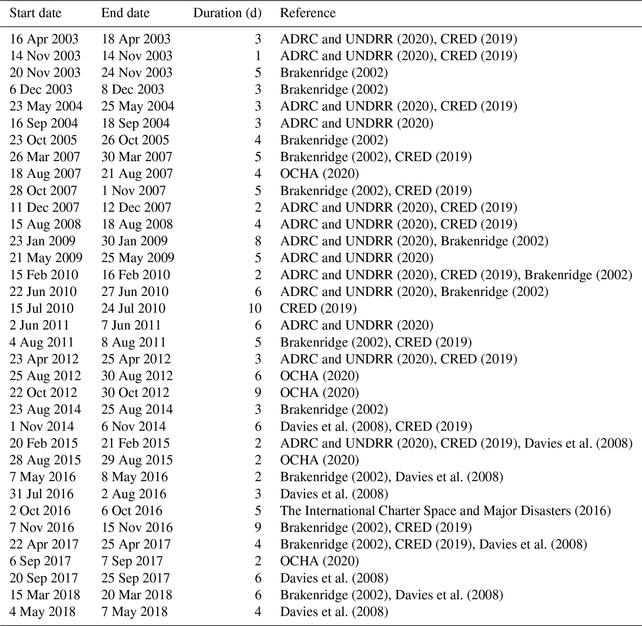
Table A2Past drought events in the Dominican Republic over the period from 2000 to 2019.

The following tables report the performances of NN (Table B1) and SVM (Table B2) in drought event identification when using different SPI accumulation periods.
Table B1NN metrics median value of the top 5 % configuration according to F1 score.

Table B2SVM metrics median value of the top 5 % configuration according to F1 score.
The six rainfall datasets (CCS, CHIRPS, CMORPH, GSMaP, IMERG and PERSIANN) and the soil moisture dataset (ERA5) are freely available at the links cited in the references.
All authors contributed to the conceptual design of this study. LC and RF designed the modelling framework. LC implemented the models and ran the analyses. All authors analysed and discussed the results. LC, RF and BM wrote the manuscript with the support of MLVM. All authors reviewed the manuscript before submission to the journal.
The authors declare that they have no conflict of interest.
Publisher's note: Copernicus Publications remains neutral with regard to jurisdictional claims in published maps and institutional affiliations.
This article is part of the special issue “Groundbreaking technologies, big data, and innovation for disaster risk modelling and reduction”. It is not associated with a conference.
This work was supported by the Disaster Risk Financing Challenge Fund, through SMART: A Statistical Machine Learning Framework for Parametric Risk Transfer; base funding UIDB/04708/2020 of the CONSTRUCT – Instituto de I&D em Estruturas e Construções, funded by national funds through the Portuguese FCT/MCTES (PIDDAC); and the Italian Ministry of Education, within the framework of the project Dipartimenti di Eccellenza at IUSS Pavia.
This paper was edited by Paolo Tarolli and reviewed by two anonymous referees.
Abadi, M., Agarwal, A., Barham, P., Brevdo, E., Chen, Z., Citro, C., Corrado, G. S., Davis, A., Dean, J., Devin, M., Ghemawat, S., Goodfellow, I., Harp, A., Irving, G., Isard, M., Jia, Y., Jozefowicz, R., Kaiser, L., Kudlur, M., Levenberg, J., Mane, D., Monga, R., Moore, S., Murray, D., Olah, C., Schuster, M., Shlens, J., Steiner, B., Sutskever, I., Talwar, K., Tucker, P., Vanhoucke, V., Vasudevan, V., Viegas, F., Vinyals, O., Warden, P., Wattenberg, M., Wicke, M., Yu, Y., and Zheng, X.: TensorFlow: Large-Scale Machine Learning on Heterogeneous Distributed Systems, arXiv [preprint], arXiv:1603.04467, 2016. a
ADRC and UNDRR: GLIDE number, available at: https://glidenumber.net/glide/public/search/search.jsp (last access: 21 June 2020), Asian Disaster Reduction Centre (ADRC), Kobe, Japan, 2020. a, b, c, d, e, f, g, h, i, j, k, l, m
African Union: African Risk Capacity: Transforming disaster risk management & financing in Africa, available at: https://www.africanriskcapacity.org/ (last access: 21 June 2020), 2021. a
Aksoy, S. and Haralick, R. M.: Feature normalization and likelihood-based similarity measures for image retrieval, Pattern Recogn. Lett., 22, 563–582, https://doi.org/10.1016/S0167-8655(00)00112-4, 2001. a
Alipour, A., Ahmadalipour, A., Abbaszadeh, P., and Moradkhani, H.: Leveraging machine learning for predicting flash flood damage in the Southeast US, Environ. Res. Lett., 15, 024011, https://doi.org/10.1088/1748-9326/ab6edd, 2020. a
Awondo, S. N.: Efficiency of Region-wide Catastrophic Weather Risk Pools: Implications for African Risk Capacity Insurance Program, J. Dev. Econ., 136, 111–118, https://doi.org/10.1016/j.jdeveco.2018.10.004, 2018. a
Barnett, B. J. and Mahul, O.: Weather index insurance for agriculture and rural areas in lower-income countries, Am. J. Agr. Econ., 89, 1241–1247, https://doi.org/10.1111/j.1467-8276.2007.01091.x, 2007. a
Barredo, J. I.: Major flood disasters in Europe: 1950–2005, Nat. Hazards, 42, 125–148, https://doi.org/10.1007/s11069-006-9065-2, 2007. a
Black, E., Tarnavsky, E., Maidment, R., Greatrex, H., Mookerjee, A., Quaife, T., and Brown, M.: The use of remotely sensed rainfall for managing drought risk: A case study of weather index insurance in Zambia, Remote Sens.-Basel, 8, 342, https://doi.org/10.3390/rs8040342, 2016. a, b
Bolvin, D. T., Braithwaite, D., Hsu, K., Joyce, R., Kidd, C., Nelkin, E. J., Sorooshian, S., Tan, J., and Xie, P.: NASA Global Precipitation Measurement (GPM) Integrated Multi-satellitE Retrievals for GPM (IMERG). Algorithm Theoretical Basis Document (ATBD) Version 5.2, Tech. rep., available at: https://pmm.nasa.gov/sites/default/files/document_files/IMERG_ATBD_V5.2_0.pdf (last access: 21 June 2020), NASA, 2018. a
Boser, B. E., Vapnik, V. N., and Guyon, I. M.: Training Algorithm Margin for Optimal Classifiers, COLT92: 5th Annual Workshop on Computational Learning Theory, Pittsburgh, Pennsylvania, USA, 27–29 July 1992, 144–152, 1992. a
Bowden, G. J., Dandy, G. C., and Maier, H. R.: Input determination for neural network models in water resources applications. Part 1 – Background and methodology, J. Hydrol., 301, 75–92, https://doi.org/10.1016/j.jhydrol.2004.06.021, 2005. a
Brakenridge, G.: Global Active Archive of Large Flood Events, available at: http://floodobservatory.colorado.edu/Archives/index.html (last access: 21 June 2020), 2002. a, b, c, d, e, f, g, h, i, j, k, l, m, n
Calvet, L., Lopeman, M., de Armas, J., Franco, G., and Juan, A. A.: Statistical and machine learning approaches for the minimization of trigger errors in parametric earthquake catastrophe bonds, SORT, 41, 373–391, https://doi.org/10.2436/20.8080.02.64, 2017. a
Castillo, M. J., Boucher, S., and Carter, M.: Index Insurance : Using Public Data to Benefit Small-Scale Agriculture, Int. Food Agribus. Man., 19, 93–114, 2016. a
Chantarat, S., Mude, A. G., Barrett, C. B., and Carter, M. R.: Designing Index-Based Livestock Insurance for Managing Asset Risk in Northern Kenya, J. Risk Insur., 80, 205–237, https://doi.org/10.1111/j.1539-6975.2012.01463.x, 2013. a
Chawla, N. V., Bowyer, K. W., Hall, L. O., and Kegelmeyer, W. P.: SMOTE: Synthetic Minority Over-sampling Technique, J. Artif. Intell. Res., 16, 321–357, https://doi.org/10.1613/jair.953, 2002. a
Chen, T., Ren, L., Yuan, F., Tang, T., Yang, X., Jiang, S., Liu, Y., Zhao, C., and Zhang, L.: Merging ground and satellite-based precipitation data sets for improved hydrological simulations in the Xijiang River basin of China, Stoch. Env. Res. Risk A., 33, 1893–1905, https://doi.org/10.1007/s00477-019-01731-w, 2019. a
Chiang, Y.-M., Hsu, K.-L., Chang, F.-J., Hong, Y., and Sorooshian, S.: Merging multiple precipitation sources for flash flood forecasting, J. Hydrol., 340, 183–196, https://doi.org/10.1016/j.jhydrol.2007.04.007, 2007. a, b
Cornell University: CSF Caribbean Drought Atlas, available at: http://climatesmartfarming.org/tools/caribbean-drought/ (last access: 21 June 2020), 2018. a
CRED: EM-DAT: The International Disaster Database, available at: http://www.emdat.be/database. (last access: 21 June 2020), Centre for Research on the Epidemiology of Disasters – CRED, Brussels, Belgium, 2019. a, b, c, d, e, f, g, h, i, j, k, l, m, n, o, p, q
Crone, S. F., Lessmann, S., and Stahlbock, R.: The impact of preprocessing on data mining: An evaluation of classifier sensitivity in direct marketing, Eur. J. Oper. Res., 173, 781–800, https://doi.org/10.1016/j.ejor.2005.07.023, 2006. a
Davies, R., Behrend, J., and Hill, E.: FloodList, available at: http://floodlist.com/ (last access: 21 June 2020), Copernicus, 2008. a, b, c, d, e, f, g, h
Dreyfus, G.: Neural Networks: Methodology and Applications, Springer Science & Business Media, 2005. a
Eckstein, D., Künzel, V., and Schäfer, L.: Global Climate Risk Index 2018. Who Suffers Most From Extreme Weather Events? Weather-related Loss Events in 2016 and 1997 to 2016, Tech. rep., Germanwatch, available at: http://www.germanwatch.org/en/cri (last access: 21 June 2020), 2017. a
ECMWF, Copernicus, and Climate Change Service: ERA5 hourly data on single levels from 1979 to present, https://doi.org/10.24381/cds.adbb2d47, 2018. a
European Drought Observatory: Standardized Precipitation Index (SPI), available at: https://edo.jrc.ec.europa.eu/ (last access: 21 June 2020), 2020. a
Felix, E. A. and Lee, S. P.: Systematic literature review of preprocessing techniques for imbalanced data, IET Softw., 13, 479–496, https://doi.org/10.1049/iet-sen.2018.5193, 2019. a
Field, C., Barros, V., Dokken, D., Mach, K., Mastrandrea, M., Bilir, T., Chatterjee, M., Ebi, K., Estrada, Y., Genova, R., Girma, B., Kissel, E., Levy, A., MacKracken, S., Mastrandrea, P., White, L., and IPCC: Climate Change 2014: Impacts, Adaptation, and Vulnerability: Summaries, Frequently Asked Questions, and Cross-Chapter Boxes: A Working Group II Contribution to the Fifth Assessment Report of the Intergovernmental Panel on Climate Change, World Meteorological Organization, Geneva, 2014. a
Figueiredo, R., Martina, M. L. V., Stephenson, D. B., and Youngman, B. D.: A Probabilistic Paradigm for the Parametric Insurance of Natural Hazards, Risk Anal., 38, 2400–2414, https://doi.org/10.1111/risa.13122, 2018. a, b, c, d, e
Flach, P. A. and Kull, M.: Precision-Recall-Gain curves: PR analysis done right, Adv. Neur. In., 2015-Januar, 838–846, 2015. a
Franco, G.: Minimization of trigger error in cat-in-a-box parametric earthquake catastrophe bonds with an application to Costa Rica, Earthq. Spectra, 26, 983–998, https://doi.org/10.1193/1.3479932, 2010. a
Fung, K. F., Huang, Y. F., Koo, C. H., and Soh, Y. W.: Drought forecasting: A review of modelling approaches 2007–2017, J. Water Clim. Change, 11, 771–799, https://doi.org/10.2166/wcc.2019.236, 2019. a, b
Funk, C., Peterson, P., Landsfeld, M., Pedreros, D., Verdin, J., Shukla, S., Husak, G., Rowland, J., Harrison, L., Hoell, A., and Michaelsen, J.: The climate hazards infrared precipitation with stations–a new environmental record for monitoring extremes, Scientific Data, 2, 150066, https://doi.org/10.1038/sdata.2015.66, 2015. a
Gagne, D., McGovern, A., Haupt, S., Sobash, R., Williams, J., and Xue, M.: Storm-Based Probabilistic Hail Forecasting with Machine Learning Applied to Convection-Allowing Ensembles, Weather Forecast., 32, 1819–1840, https://doi.org/10.1175/WAF-D-17-0010.1, 2017. a
Garcia, V., Sanchez, J. S., and Mollineda, R. A.: On the effectiveness of preprocessing methods when dealing with different levels of class imbalance, Knowl.-Based Syst., 25, 13–21, https://doi.org/10.1016/j.knosys.2011.06.013, 2012. a
Ghahramani, Z.: Unsupervised learning, chap. 5, in: Advanced Lectures on Machine Learning, edited by: Bousquet, O., von Luxburg, U., and Ratsch, G., Springer-Verlag Berlin Heidelberg, Tübingen, i edn., pp. 72–112, 2004. a
Global Disaster Alert and Coordination System: Overall Orange alert Drought for Hispaniola-2019, available at: https://www.gdacs.org/report.aspx?eventtype=DR&eventid=1012765&episodeid=7 (last access: 21 June 2020), 2018. a
Guo, C., Pleiss, G., Sun, Y., and Weinberger, K. Q.: On calibration of modern neural networks, 34th International Conference on Machine Learning, ICML 2017, 3, 2130–2143, 6 August 2017–11 August 2017, International Convention Centre Sydney, Sydney, Australia, 2017. a
Hao, Z., Singh, V. P., and Xia, Y.: Seasonal Drought Prediction: Advances, Challenges, and Future Prospects, Rev. Geophys., 56, 108–141, https://doi.org/10.1002/2016RG000549, 2018. a, b
Herrera, D. and Ault, T. R.: Insights from a New High-Resolution Drought Atlas for the Caribbean spanning 1959 to 2016, B. Am. Meteorol. Soc., 30, 7801–7825, https://doi.org/10.1175/JCLI-D-16-0838.1, 2017. a
Hoeppe, P.: Trends in weather related disasters: Consequences for insurers and society, Weather and Climate Extremes, 11, 70–79, https://doi.org/10.1016/j.wace.2015.10.002, https://doi.org/10.1016/j.wace.2015.10.002, 2016. a
Hong, Y., Hsu, K. L., Sorooshian, S., and Gao, X.: Precipitation estimation from remotely sensed imagery using an artificial neural network cloud classification system, J. Appl. Meteorol., 43, 1834–1852, https://doi.org/10.1175/jam2173.1, 2004. a
Hossin, M. and Sulaiman, M.: A Review on Evaluation Metrics for Data Classification Evaluations, International Journal of Data Mining & Knowledge Management Process, 5, 01–11, https://doi.org/10.5121/ijdkp.2015.5201, 2015. a
Huang, J., Li, Y. F., and Xie, M.: An empirical analysis of data preprocessing for machine learning-based software cost estimation, Inform. Softw. Tech., 67, 108–127, https://doi.org/10.1016/j.infsof.2015.07.004, 2015. a
Ibarra, H. and Skees, J.: Innovation in risk transfer for natural hazards impacting agriculture., Environmental Hazards, 7, 62–69, https://doi.org/10.1016/j.envhaz.2007.04.008, 2007. a
Izzo, M., Rosskopf, C. M., Aucelli, P. P. C., Maratea, A., Méndez, R., Pérez, C., and Segura, H.: A New Climatic Map of the Dominican Republic Based on the Thornthwaite Classification, Phys. Geogr., 31, 455–472, https://doi.org/10.2747/0272-3646.31.5.455, 2010. a
Jones, K. S. and Van Rijsbergen, C. J.: Progress in documentation: Information retrieval test collections, J. Doc., 32, 59–75, https://doi.org/10.1108/eb026616, 1976. a
Joyce, R. J., Janowiak, J. E., Arkin, P. A., and Xie, P.: CMORPH: A method that produces global precipitation estimates from passive microwave and infrared data at high spatial and temporal resolution, J. Hydrometeorol., 5, 487–503, https://doi.org/10.1175/1525-7541(2004)005<0487:CAMTPG>2.0.CO;2, 2004. a
Khalaf, M., Hussain, A. J., Al-Jumeily, D., Baker, T., Keight, R., Lisboa, P., Fergus, P., and Al Kafri, A. S.: A Data Science Methodology Based on Machine Learning Algorithms for Flood Severity Prediction, 2018 IEEE Congress on Evolutionary Computation, CEC 2018 – Proceedings, pp. 1–8, 8–13 July 2018, Rio de Janeiro, Brazil, https://doi.org/10.1109/CEC.2018.8477904, 2018. a
Kim, M., Park, M., Im, J., Park, S., and Lee, M.: Machine Learning Approaches for Detecting Tropical Cyclone Formation Using Satellite Data, Remote Sens.-Basel, 11, 1195, https://doi.org/10.3390/rs11101195, 2019. a
Kron, W., Löw, P., and Kundzewicz, Z. W.: Changes in risk of extreme weather events in Europe, Environ. Sci. Policy, 100, 74–83, https://doi.org/10.1016/j.envsci.2019.06.007, 2019. a
Krzanowski, W. and Hand, D. J.: ROC Curves for Continuous Data, vol. 111, Chapman and Hall/CRC, Boca Raton, FL, https://doi.org/10.1201/9781439800225, 2009. a
Kunreuther, H.: Mitigation and Financial Risk Management for Natural Hazards A Risk Management Strategy for Reducing Losses and Providing Financial Protection, The Geneva Papers on Risk and Insurance. Issues and Practice, 26, 277–296, 2001. a
Ling, C. and Li, C.: Data Mining for Direct Marketing: Problems and Solutions, American Association for Artificial Intelligence, 73–79, Proceedings of the Fourth International Conference on Knowledge Discovery and Data Mining, New York, NY, USA, 1998. a
Loew, A., Bell, W., Brocca, L., Bulgin, C. E., Burdanowitz, J., Calbet, X., Donner, R. V., Ghent, D., Gruber, A., Kaminski, T., Kinzel, J., Klepp, C., Lambert, J. C., Schaepman-Strub, G., Schröder, M., and Verhoelst, T.: Validation practices for satellite-based Earth observation data across communities, Rev. Geophys., 55, 779–817, https://doi.org/10.1002/2017RG000562, 2017. a
Maini, V. and Sabri, S.: Machine Learning for Humans, available at: https://everythingcomputerscience.com/books/Machine Learning for Humans.pdf (last access: 21 June 2020), 2017. a
Makaudze, E. M. and Miranda, M. J.: Catastrophic drought insurance based on the remotely sensed normalised difference vegetation index for smallholder farmers in Zimbabwe, Agricultural Economics Research, Policy and Practice in Southern Africa, 49, 418–432, https://doi.org/10.1080/03031853.2010.526690, 2010. a
Mas, J. F. and Flores, J. J.: The application of artificial neural networks to the analysis of remotely sensed data, Int. J. Remote Sens., 29, 617–663, https://doi.org/10.1080/01431160701352154, 2008. a
Massaron, J. P. and Muller, L.: Machine learning for dummiers, vol. 11, John Wiley & Sons, Inc., 2016. a
McClure, N.: TensorFlow Machine Learning, available at: https://www.tensorflow.org/federated (last access: 21 June 2020), 2017. a
McKee, T. B., Doesken, N. J., and Kleist, J.: The relationship of drought frequency and duration to time scales, in: AMS 8th Conference on Applied Climatology, January, Anaheim, California, 17–22 January 1993, available at: https://www.droughtmanagement.info/literature/AMS_Relationship_Drought_Frequency_Duration_Time_Scales_1993.pdf (last access: 21 June 2020), pp. 179–184, 1993. a, b
Mosavi, A., Ozturk, P., and Chau, K. W.: Flood prediction using machine learning models: Literature review, Water (Switzerland), 10, 1536, https://doi.org/10.3390/w10111536, 2018. a, b
Mosteller, F. and Tukey, J. W.: Data analysis, including statistics, in: Handbook of social psychology, edited by: Lindzey, G. and Aronson, E., Addison-Wesley, 2, 80–203, 1968. a
Murphy, A. H. and Ehrendorfer, M.: On the Relationship between the Accuracy and Value of Forecasts in the Cost-Loss Ratio Situation, Weather Forecast., 2, 243–251, https://doi.org/10.1175/1520-0434(1987)002<0243:OTRBTA>2.0.CO;2, 1987. a
Nayak, M. A. and Ghosh, S.: Prediction of extreme rainfall event using weather pattern recognition and support vector machine classifier, Theor. Appl. Climatol., 114, 583–603, https://doi.org/10.1007/s00704-013-0867-3, 2013. a, b
OCHA: ReliefWeb, available at: https://reliefweb.int/ (last access: 21 June 2020), OCHA United Nations Office for the Coordination of Humanitarian Affairs, 2020. a, b, c, d, e
Ornella, L., Kruseman, G., and Crossa, J.: Satellite Data and Supervised Learning to Prevent Impact of Drought on Crop Production: Meteorological Drought, in: Drought: Detection and Solutions, edited by: Ondrasek, G., IntechOpen, London, UK, https://doi.org/10.5772/57353, 2019. a
Payano-Almanzar, R. and Rodriguez, J.: Meteorological, Agricultural and Hydrological Drought in the Dominican Republic: A review, Current World Environment, 13, 124–143, https://doi.org/10.12944/CWE.13.1.12, 2018. a, b, c, d, e
Pedregosa, F., Varoquaux, G., Buitinck, L., Louppe, G., Grisel, O., and Mueller, A.: Scikit-learn: Machine Learning in Python, J. Mach. Learn. Res., 12, 2825–2830, 2011. a
Plate, E.: Flood risk and flood management, J. Hydrol., 267, 2–11, https://doi.org/10.1016/S0022-1694(02)00135-X, 2002. a
Platt, J. C.: Probabilistic Outputs for Support Vector Machines and Comparisons to Regularized Likelihood Methods, in: Advances in Large Margin Classifiers, edited by: Smola, A. J., Bartlett, P. L., Scholkopf, B., and Schuurmans, D., MIT Press, Cambridge, Massachusetts, USA, pp. 61–74, 1999. a
Richman, M. B., Leslie, L. M., and Segele, Z. T.: Classifying Drought in Ethiopia Using Machine Learning, Procedia Comput. Sci., 95, 229–236, https://doi.org/10.1016/j.procs.2016.09.319, 2016. a
Saito, T. and Rehmsmeier, M.: The precision-recall plot is more informative than the ROC plot when evaluating binary classifiers on imbalanced datasets, PLoS ONE, 10, 1–21, https://doi.org/10.1371/journal.pone.0118432, 2015. a, b
Sallis, P., Claster, W., and Hernandez, S.: A machine-learning algorithm for wind gust prediction, Comput. Geosci., 37, 1337–1344, https://doi.org/10.1016/j.cageo.2011.03.004, 2011. a
Samuel, A. L.: Eight-move opening utilizing generalization learning, (See Appendix B, Game G-43.1 Some Studies in Machine Learning Using the Game of Checkers), IBM Journal, pp. 210–229, 1959. a
Sorooshian, S., Hsu, K. L., Gao, X., Gupta, H. V., Imam, B., and Braithwaite, D.: Evaluation of PERSIANN system satellite-based estimates of tropical rainfall, B. Am. Meteorol. Soc., 81, 2035–2046, https://doi.org/10.1175/1520-0477(2000)081<2035:EOPSSE>2.3.CO;2, 2000. a
Stevens, E. and Antiga, L.: Deep Learning with PyTorch Essential Excerpts, Manning Publications Co., Shelter Island, New York, 2019. a, b, c
Sun, Y., Wong, A. K. C., and Kamel, M. S.: Classification of imbalanced data: A review, Int. J. Pattern Recogn., 23, 687–719, https://doi.org/10.1142/S0218001409007326, 2009. a
Surminski, S. and Oramas-Dorta, D.: Flood insurance schemes and climate adaptation in developing countries, Int. J. Disast. Risk Re., 7, 154–164, https://doi.org/10.1016/j.ijdrr.2013.10.005, 2014. a
Surminski, S., Bouwer, L., and Linnerooth-Bayer, J.: How insurance can support climate resilience, Nat. Clim. Change, 6, 333–334, https://doi.org/10.1038/nclimate2979, 2016. a
Tate, E. L. and Gustard, A.: Drought Definition: A Hydrological Perspective, in: Drought and Drought Mitigation in Europe. Advances in Natural and Technological Hazards Research, edited by: Vogt, J. V. and Somma, F., vol 14., pp. 23–48, https://doi.org/10.1007/978-94-015-9472-1_3, Springer, Dordrecht, Dordrecht, 2000. a
The International Charter Space and Major Disasters: Hurricane Matthew in the Dominican Republic, available at: https://disasterscharter.org/web/guest/activations/-/article/flood-in-dominican-republic (last access: 21 June 2020), 2016. a
The World Bank: Operational Innovations: Providing Immediate Funding After Natural Disasters, International Bank for Reconstruction and Development/The World Bank, Washington, DC, 2008. a
The World Bank: Dominican Republic, available at: https://data.worldbank.org/country/dominican-republic (last access: 21 June 2020), 2019. a
Ushio, T. and Kachi, M.: Kalman Filtering Applications for Global Satellite Mapping of Precipitation (GSMaP), in: Satellite Rainfall Applications for Surface Hydrology, edited by: Gebremichael, M. and Hossain, F., Springer Netherlands, Dordrecht, https://doi.org/10.1007/978-90-481-2915-7_7, pp. 105–123, 2010. a
Van Nostrand, J. M. and Nevius, J. G.: Parametric Insurance: Using Objective Measures to Address the Impacts of Natural Disasters and Climate Change, Environ. Claim. J., 23, 227–237, https://doi.org/10.1080/10406026.2011.607066, 2011. a
Visser, H., Petersen, A. C., and Ligtvoet, W.: On the relation between weather-related disaster impacts, vulnerability and climate change, Climatic Change, 125, 461–477, https://doi.org/10.1007/s10584-014-1179-z, 2014. a
Wang, L.: Support Vector Machines: Theory and Applications, vol. 177, first edn., Springer, 2005. a
Wilhite, D. A.: Drought as a natural hazard: Concepts and definitions, in: Drought: A Global Assessment, Drought – National Drought Mitigation Center, Nebraska, Lincoln, pp. 3–18, 2000. a
World Meteorological Organization and Global Water Partnership: Handbook of Drought Indicators and Indices, Integrated Drought Management Programme, Geneva, 2016. a
Zhang, S., Zhang, C., and Yang, Q.: Data preparation for data mining, Appl. Artif. Intell., 17, 375–381, https://doi.org/10.1080/713827180, 2003. a
- Abstract
- Introduction
- Methodology
- Case study
- Results and discussion
- Conclusions
- Appendix A: Catalogue of historical events
- Appendix B: Performance of NN and SVM in drought event identification when using different SPI accumulation periods
- Data availability
- Author contributions
- Competing interests
- Disclaimer
- Special issue statement
- Financial support
- Review statement
- References