the Creative Commons Attribution 4.0 License.
the Creative Commons Attribution 4.0 License.
 | 17 Jun 2021
Towards a compound-event-oriented climate model evaluation: a decomposition of the underlying biases in multivariate fire and heat stress hazards
Roberto Villalobos-Herrera
Emanuele Bevacqua
Andreia F. S. Ribeiro
Graeme Auld
Laura Crocetti
Bilyana Mircheva
Minh Ha
Jakob Zscheischler
Carlo De Michele
Climate models' outputs are affected by biases that need to be detected and adjusted to model climate impacts. Many climate hazards and climate-related impacts are associated with the interaction between multiple drivers, i.e. by compound events. So far climate model biases are typically assessed based on the hazard of interest, and it is unclear how much a potential bias in the dependence of the hazard drivers contributes to the overall bias and how the biases in the drivers interact. Here, based on copula theory, we develop a multivariate bias-assessment framework, which allows for disentangling the biases in hazard indicators in terms of the underlying univariate drivers and their statistical dependence. Based on this framework, we dissect biases in fire and heat stress hazards in a suite of global climate models by considering two simplified hazard indicators: the wet-bulb globe temperature (WBGT) and the Chandler burning index (CBI). Both indices solely rely on temperature and relative humidity. The spatial pattern of the hazard indicators is well represented by climate models. However, substantial biases exist in the representation of extreme conditions, especially in the CBI (spatial average of absolute bias: 21 ∘C) due to the biases driven by relative humidity (20 ∘C). Biases in WBGT (1.1 ∘C) are small compared to the biases driven by temperature (1.9 ∘C) and relative humidity (1.4 ∘C), as the two biases compensate for each other. In many regions, also biases related to the statistical dependence (0.85 ∘C) are important for WBGT, which indicates that well-designed physically based multivariate bias adjustment procedures should be considered for hazards and impacts that depend on multiple drivers. The proposed compound-event-oriented evaluation of climate model biases is easily applicable to other hazard types. Furthermore, it can contribute to improved present and future risk assessments through increasing our understanding of the biases' sources in the simulation of climate impacts.
- Article
(9331 KB) - Full-text XML
- BibTeX
- EndNote


Understanding and assessing the risk of high-impact events induced by the combination of multiple climate drivers and/or hazards, referred to as compound events, is challenging (e.g. Bevacqua et al., 2017; Manning et al., 2018; Zscheischler et al., 2020). One of the reasons is that many high-impact events are caused by multiple variables that may not be extreme themselves, but their combination leads to an extreme impact (Zscheischler et al., 2018). For example, the risks associated with combined high temperature and high/low relative humidity such as heat stress and fires can manifest in heat-related human fatalities (Raymond et al., 2020) and fire-induced tree mortality (Brando et al., 2014) even if the two contributing variables are not necessarily extreme in a statistical sense. In the future, combinations of climate variables leading to disproportionate impacts will be affected by global warming, and reliable risk assessments are required (Fischer and Knutti, 2013; Russo et al., 2017; Schär, 2016; Raymond et al., 2020; Jézéquel et al., 2020; Zscheischler et al., 2020). Therefore, a better understanding of how climate models represent the joint behaviour of variables behind compound events, such as temperature and relative humidity, is crucial to correctly quantify their associated hazards today and in the future (Zscheischler et al., 2018).
Typically, the raw climate model data contain biases, which lead to biased estimates of climate risks (Maraun et al., 2017). Evaluating, i.e. assessing and understanding, such biases is a crucial step towards impact modelling and thus assessment of future climate risks. Climate model evaluation is very often univariate; i.e. it does not take into account the multivariate nature of many hazards that are driven by the interplay of multiple contributing variables (Vezzoli et al., 2017; Zscheischler et al., 2018, 2019; Francois et al., 2020). However, evaluating the model representation of the individual contributing variables individually, and hence disregarding both the biases in the dependence between the contributing variables and how the biases in the drivers combine to influence the hazard, cannot provide direct information regarding the biases in the resulting hazard indicator. Furthermore, evaluating the hazard indicator only, e.g. heat stress regardless of the contributing variables temperature and relative humidity, may hide compensating biases in the contributing variables, even if the hazard indicator appears to be well represented. An evaluation of climate models that considers the underlying multivariate nature of the hazards can provide a better physical understanding of the relevant model skills. In turn, a better understanding of model skills can serve as a basis for better adjustment of the biases and/or selection of best-performing models, which are crucial for hazard assessment both in the present and future climate. However, studies evaluating the climate model multivariate representation of hazard indicator are still rare (Bevacqua et al., 2019; Zscheischler et al., 2021), and little is known on the effects of those biases on multivariate hazards (Fischer and Knutti, 2013; Zscheischler et al., 2018).
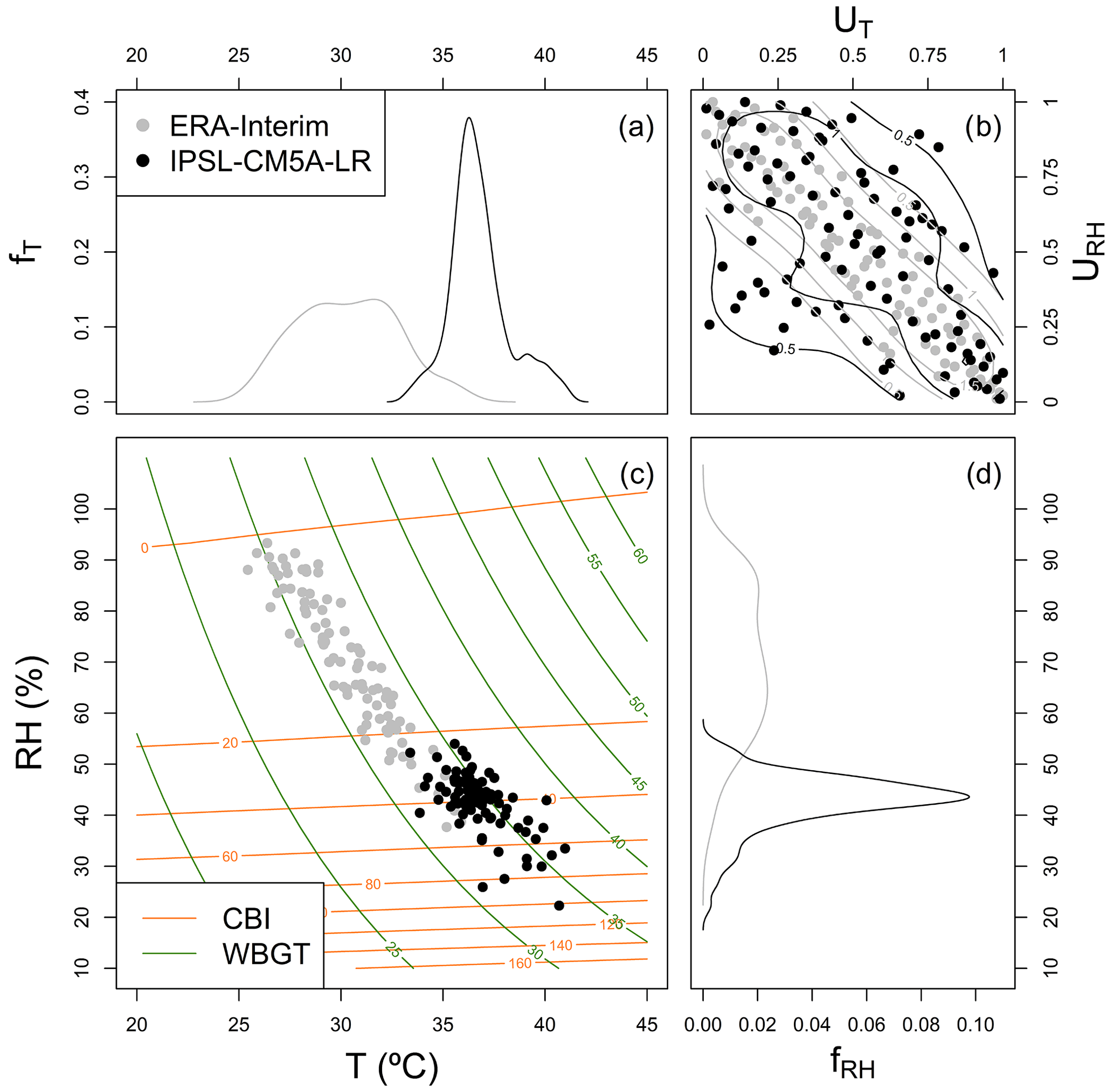
Figure 1Copula-based conceptual framework employed in this study to evaluate biases in CBI and WBGT indices. The framework is illustrated for a representative location in Brazil (Amazonia, 5∘ S and 56.5∘ W; indicated via X markers in the next figures). Panel (c) shows the bivariate distribution of T and RH based on ERA-Interim (grey) and IPSL-CM5A-LR data (black) during 1979–2005. Isolines indicate equal levels of CBI (orange) and WBGT (green). The decomposition of biases from the marginals (a, d) and the copula (b) are illustrated as the discrepancies between the black (IPSL-CM5A-LR model) and grey features (ERA-Interim).
In this study we propose a copula-based multivariate bias-assessment framework, which allows for decomposing the sources of bias in hazard indicators. We employ global climate model outputs from the fifth phase of the Coupled Model Intercomparison Project (CMIP5) and consider two simplified hazard indices, the Chandler burning index (CBI) for fire hazard and the wet-bulb globe temperature (WBGT) index for heat stress, both driven solely by temperature and relative humidity. Figure 1 illustrates the main rationale of the multivariate bias-assessment framework. Both hazard indices, CBI and WBGT, are influenced by the bivariate distribution of temperature and relative humidity (Fig. 1c). Based on copula theory, such a bivariate distribution can be decomposed in terms of the marginal distributions of temperature and relative humidity (Fig. 1a and d), as well as their statistical dependence (Fig. 1b). Hence, such a copula-based decomposition allows for understanding the biases in the hazard estimates in terms of the contribution from the marginal distributions individually (Fig. 1a and d; see difference between grey and black lines) and from their statistical dependence (Fig. 1b) (Vezzoli et al. 2017; Bevacqua et al., 2019). We present a methodology to quantify the role played by the biases in temperature, relative humidity, and their dependence in the final bias in the fire and heat stress indices as simulated by climate models.
2.1 Pre-processing
We employ 6-hourly data of 2 m air temperature (T) and relative humidity (RH) during the period 1979–2005 from ERA-Interim reanalysis (Berrisford et al., 2011; Dee et al. 2011) and 12 models from the CMIP5 multimodel ensemble (Taylor et al., 2012): ACCESS1-0, ACCESS1-3, BCC-CSM1.1-m, BNU-ESM, CNRM-CM5, GFDL-ESM2G, GFDL-ESM2M, INM-CM4, IPSL-CM5A-LR, NorESM1-M, GFDL-CM3, and IPSL-CM5A-MR; leap days were removed. To allow for an intermodel comparison, data were bilinearly interpolated to a 2.5∘ by 2.5∘ regular latitude–longitude grid. All oceanic grid cells as well as those beneath 60∘ S were removed from all analyses, given that arguably no heat stress and fire risk exists in these areas.
Following Zscheischler et al. (2019), we restrict our analysis to the hottest calendar month of the year, which is selected based on the climatology of ERA-Interim data at each grid point. This choice was made because arguably heat stress and fire hazards tend to be more frequent during the warmest period of the year, and it avoids dealing with seasonality; however we note that this assumes that CMIP5 models correctly reproduce the seasonality observed in ERA-Interim. Finally, for each model and location, we consider the T and RH values at the daily 6-hourly time steps corresponding to the daily maximum temperature within the hottest month. The above results in a time series for each location and model, with daily values of the pair (T, RH).
The resulting time series data are autocorrelated, which can compromise the interpretation of the statistical tests that we apply in the analysis (Yue et al., 2002; Dale and Fortin, 2009). Therefore, we carry out the analysis on the decorrelated time series, which are obtained from the original through subsampling every N = 9 d, where N is the lag required to remove the autocorrelation in T and RH time series data everywhere (at 95 % confidence level). The value of N was determined as follows: for all individual grid points and years in ERA-Interim and the CMIP5 models, the autocorrelation function was calculated; then, the minimum lag for which the autocorrelation was non-significant at the 95 % confidence level was determined. Finally, the maximum of all the minimum lags was selected, resulting in N = 9 d. The time series for all models and locations are sampled with the frequency of N. This is done N times using different start epochs, where the first sampled time series starts with time epoch one, the second sampled time series with time epoch two, and so on up to nine. The decorrelated time series of T and RH will henceforth be simply referred to as samples in the following sections.
In the Appendix, Fig. A1 illustrates, for a representative location in Brazil, one of the nine resulting samples of T and RH for ERA-Interim and for a selection of CMIP5 models. The figure also shows how the bivariate interaction of these variables drives the fire and heat stress indices (coloured isolines) introduced in the next section.
2.2 Fire hazard and heat stress indices
We quantify fire and heat stress hazards based on two indices, i.e. CBI and WBGT, respectively. While more advanced and sophisticated indices exist for both of these hazards (e.g. Van Wagner, 1987; Fiala et al., 2011), here we employ these two simplified indices. Our aim is to provide a methodological framework for a compound-event-oriented evaluation of hazard indicators. Hence, employing simplified indices allows for the development of a test case of the methodological framework. We do not aim at providing an accurate assessment of the hazard; nevertheless, our results will provide indications that can serve as a basis for follow-up studies of more complex fire and heat stress hazards.
The CBI index was employed, for example, for studying fire risk in the United States (McCutchan and Main, 1989) and globally (Roads et al., 2008). The index is based on air T (∘C) and RH (%):
The “simplified WBGT” (from now on WBGT for the sake of brevity) index was developed by the American College of Sports Medicine (ACSM, 1984) as an indicator of heat stress for average daytime conditions outdoors. The index is defined as
where is water vapour pressure (expressed in hPa), which depends on air temperature and relative humidity. More details on the definitions of the CBI and WBGT are available at McCutchan and Main (1989) and ACSM (1984).
This section presents the conceptual framework and a bias decomposition methodology used to analyse the multivariate indices described above. We then present an overview of the data processing before detailing the conventional statistical tests we have incorporated into our test suite.
3.1 Copula-based conceptual framework
As both CBI and WBGT are functions of T and RH, it follows that their distributions are determined by the joint distribution of T and RH. Copula theory provides us with a natural way to decompose the joint distribution of T and RH in terms of the marginal distributions of T and RH (the distributions of the individual variables considered in isolation) and a term, known as the copula, that describes the dependence between T and RH (Fig. 1). This allows us to understand how bias in each of these components contributes to the bias in CBI and WBGT.
A copula is a function that completely characterizes the dependence structure between random variables, in our case T and RH. Sklar's theorem (Sklar, 1959) is a fundamental result in copula theory, which states that the joint distribution of the random variables is determined by the marginal distributions and their copula. Mathematically, in our bivariate case, given the two variables T and RH, with marginal cumulative distribution functions (CDFs) FT and FRH, and marginal probability density functions (PDFs) fT and fRH, following Sklar's theorem, the joint PDF fT,RH can be decomposed as
where URH=FRH(RH), UT=FT(T) (note that U indicates that both URH and UT are uniformly distributed by construction on the domain [0,1]), and c is the copula density, which describes the dependence of the joint distribution fT,RH independently from the marginal distributions fT and fRH. Note that Eq. (3) naturally extends to the case of an arbitrary number of random variables (Bevacqua et al., 2017); however here we focus on the bivariate case. Copulas allow for great flexibility in modelling complex dependence structures between several variables, and there are a huge variety of parametric copula families available for statistical modelling purposes (Nelsen, 2006; Salvadori and De Michele, 2007; Salvadori et al., 2007; Durante and Sempi, 2015; Bevacqua et al., 2020a). However, note that following the methodologies developed by Rémillard and Scaillet (2009) and Vezzoli et al. (2017), here we will consider a non-parametric framework; i.e. we will consider empirical, rather than parametric, distributions within our testing procedures. This choice avoids unnecessary parametric-based assumptions on the distributions that could bias the results about both univariate and multivariate features.
A characteristic of copulas is the invariance property (Salvadori et al. 2007, proposition 3.2); i.e. if g1 and g2 are monotonic (increasing) functions, then the transformed variables g1(T) and g2(RH) have the same copula as T and RH. This property is crucial to the methodology described in the following section, where the monotonic functions are the marginal CDFs of T and RH (or their inverses).
3.2 Contribution of the bias in the drivers to the bias of CBI and WBGT
We assess how biases in each of the marginal distributions of Tmod and RHmod, and Cmod (the copula of Tmod and RHmod), contribute to the bias in the representation of the extreme values of CBI and WBGT (extremes are defined based on 95th percentiles (Q95)). This is achieved based on a methodology originally introduced by Bevacqua et al. (2019) to attribute changes in compound flooding to its underlying drivers (and employed by for example Manning et al., 2019, and Bevacqua et al., 2020b).
We carried out three experiments. In experiment i, we obtained, via a data transformation, a bivariate pair (Ti, RHi) with copula Ci, where one component of the three underlying distributions (Ti, RHi, Ci) is the same as that of a given CMIP5 model, and the other two components are the same as ERA-Interim. We then perform the quantile tests described in Sect. 3.3.3 for CBI (or WBGT) using values based on (Ti, RHi) and (Terai, RHerai). The specific experiments carried out are described below.
Experiment (a) assesses the bias contribution of Tmod. From the variable Terai we calculated the uniformly distributed transformed random variable (Terai). From the variable Tmod we calculated the empirical CDF FT,mod, through which we defined ). The variable Ta has the same distribution as Tmod, while the pair (Ta, RHerai) has the copula of ERA-Interim.
Experiment (b) assesses the bias contribution of RHmod. This experiment follows the same structure as Experiment (a) but with the roles of Terai and RHerai reversed, from which we get the pairs (Terai, RHb).
Experiment (c) assesses the bias contribution of Cmod. From the variables Tmod and RHmod we calculated the associated marginal empirical cumulative distributions (UT,mod, URH,mod). From the variables Terai and RHerai, we defined the empirical CDFs FT,erai and FRH,erai, through which we defined ) and ). The pair of variables (Tc, RHc) have the same marginal distributions as the pair (Terai, RHerai), but the copula of the model, i.e. Cmod, since (Tc, RHc) was obtained from (Tmod, RHmod) by monotonic transformations of the margins.
3.3 Description of the testing procedure
The full data processing procedure is shown in Fig. A2. We began with the ERA-Interim and CMIP5 data and obtained T and RH samples (see Sect. 2.1). The CMIP5 samples were then subject to the transformation procedure described in Sect. 3.2.4. This results in five sets of T and RH data corresponding to the ERA-Interim reference, the original model sample, and the three experiments (a, b, and c) used to assess the bias contributions of biases in CMIP5 model T, RH, and their copula. At this stage, the CBI and WBGT indices are calculated on all five sets.
We execute univariate and multivariate non-parametric statistical tests to evaluate the properties of CBI, WBGT, and their driver variables (i.e. T, RH, and their dependence) prior to proceeding with our bias decomposition approach. Details for each of the tests are provided below, but, in general, we follow a non-parametric approach similar to Vezzoli et al. (2017). Each of the nine decorrelated ERA-Interim samples was independently tested on a cell-by-cell basis against a different CMIP5 model sample; therefore each statistical test is repeated nine times per model. To adjust for multiple testing, we use the conservative Bonferroni correction method, which penalizes the significance level α using the number of repeated tests m=9, so that the individual hypothesis tests are evaluated at an significance level (Jafari and Ansari-Pour, 2019). A 5 % significance level is used, after which the Bonferroni correction was adjusted to 0.0056 for use in each individual hypothesis test. All of our analysis was carried out in R (R Core Team, 2019), and the functions used for each test are detailed in their corresponding section below.
Graphically, the statistical test results are presented as a percentage of all 108 CMIP5 model samples (9 samples times 12 models) where the null hypothesis is rejected. The percentage we consider is calculated at each grid cell, and stippling is added where the null hypothesis is rejected in at least 75 % () of all CMIP5 model samples.
3.3.1 Univariate evaluation of T, RH, CBI, and WBGT
In order to understand how faithfully the marginal distributions of T, RH, CBI, and WBGT from the ERA-Interim data are represented in a given CMIP5 model, we perform the two-sample Anderson–Darling (AD) test via the ad.test function of the kSamples R package (v1.2-9; Scholz and Zhu, 2019). This is a non-parametric procedure that considers the null hypothesis: “the two samples are from the same distribution”.
3.3.2 Dependence between T and RH
A simple way to test how well the dependence between the variables T and RH in ERA-Interim is represented in a given CMIP5 model is to compare the calculated values of some statistical measure of association. Here we use Kendall's τ rank correlation. The cor.test function of the core stats R package was used to perform all τ calculations (R Core Team, 2019).
To test whether the values of τ obtained from a given model sample differ in a statistically significant way from the corresponding ERA-Interim values, we begin by considering the approximate 100(1−α) % confidence interval (τL,τU) for τ associated with the point estimator given by
where is an estimator of and is the quantile of the standard normal distribution for (Hollander et al., 2014). For our testing we calculate , , and the confidence interval (τL,τU) for each grid cell in all ERA-Interim samples, using a customized version of the kendall.ci function included in the NSM3 R package (v1.15, Schneider et al., 2020). The CMIP5 model samples are then evaluated in two ways. Firstly, if the model sample value of τ lies within the confidence interval calculated for its corresponding ERA-Interim sample, the model sample is judged to not significantly differ from ERA-Interim in terms of the rank correlation between T and RH. Secondly, we calculated the and hence the α or p value for each sample; these were tested for significance using the same Bonferroni-adjusted value of 0.0056 used in the univariate testing. The results from both testing methodologies are consistent with each other, we present the ad hoc p-value test results in the main text, and the confidence interval tests are included in the Appendix.
Note that different copulas may give rise to the same value of τ; therefore we cannot conclude that a model that faithfully reproduces the ERA-Interim values of τ is accurately representing the full dependence structure between T and RH. Therefore, we account for differences in the dependence structure by also carrying out hypothesis tests which are based on the full copula function. We perform the non-parametric test of copula equality based on the Cramér–von Mises test statistic proposed by Remillard and Scaillet (2009), used in Vezzoli et al. (2017) for testing the capability of a climate–hydrology model to reproduce the dependence between temperature, precipitation, and discharge for the Po river basin in Italy, and recently employed by Zscheischler and Fischer (2020) for evaluating the ability of climate models to represent the dependence between temperature and precipitation in Germany. The copula equality test has a null hypothesis of H0: Cerai=Cmod, where Cerai and Cmod are the copulas of T and RH represented in ERA-Interim and a given model, respectively, with the alternative hypothesis being that these copulas differ. Unlike the AD test, which can evaluate CMIP5 model performance in reproducing a single marginal distribution, the copula equality test was specifically developed to test whether two empirical copulas are equal and thus evaluates the capacity of models to reproduce the full dependency structure between T and RH. We used the TwoCop function of the TwoCop R package (v1.0, Remillard and Plante, 2012) to run the test.
3.3.3 Bias in the representation of extreme events of CBI and WBGT
To evaluate how well CMIP5 models simulate extreme values of CBI and WBGT, we compare high quantiles (i.e. the 95th percentile Q95) of these indices from each model with those of ERA-Interim. To assess whether the observed differences in the quantiles are statistically significant, we calculate the 95 % confidence intervals for the Q95 of CBI and WBGT at each location for ERA-Interim based on 1000 bootstrap samples. Like our evaluation of Kendall's τ, if the model index lies outside the confidence interval, we consider the model has a significantly different representation of extreme values of CBI and WBGT from ERA-Interim.
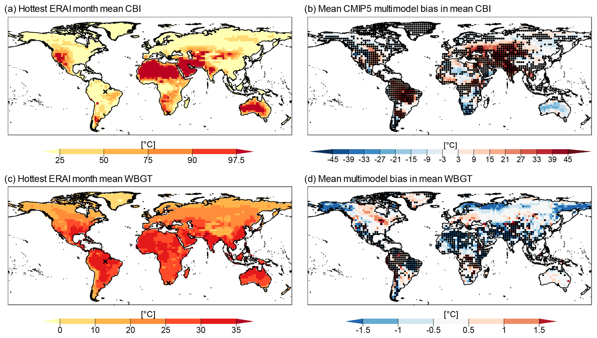
Figure 2Mean fire hazard index (CBI) value for ERA-Interim (a), and mean multimodel bias in mean CBI (b). Note that the palette is non-linear, as it follows typical defined ranges of fire hazard levels based on the CBI, i.e. very low, low, moderate, high, very high, and extreme. Mean heat stress index (WBGT) value for ERA-Interim (c), and mean multimodel bias in mean WBGT (d). Stippling indicates locations where at least 75 % of CMIP5 models failed the AD two-sample test between the CMIP5 and ERA-Interim distributions of CBI and WBGT. Bias was calculated as (CMIP5 minus ERA-Interim).
4.1 Univariate evaluation of T, RH, CBI, and WBGT
4.1.1 CBI and WBGT
We began our analysis by visualizing the multimodel mean of the mean values of CBI and WBGT during the hottest months. According to reanalysis, the mean CBI is highest in regions with dry and warm weather during the hottest month, such as the Sahara, most of Australia, and the western USA and Mexico (Fig. 2a). In contrast, CBI tends to be low in humid and warm regions such as the Amazon and Congo basins. We move to evaluating the CMIP5 model biases in mean CBI, which appear large in magnitude (compare Fig. 2b and a); most land masses are covered in dark red or blue colours, indicating CMIP5 multimodel mean bias of over 10 ∘C from the ERA-Interim. In addition, AD test results show that 59 % of the global land mass has significant differences between ERA-Interim and CMIP5 distributions of CBI in at least 75 % of model samples. Despite such biases in the representation of the mean CBI magnitude, the overall spatial patterns in mean CBI are well reproduced by the models. In fact, the area-weighted pattern correlation (Pfahl et al., 2017), from now on pattern correlation, between models and reanalysis of mean CBI is high for all CMIP5 models, with a minimum value of 0.77 for the BCC-CSM1.1-m model (Fig. A3a shows the multimodel mean of mean CBI).
In the reanalysis data, mean WBGT values over 30 ∘C are reached over most tropical land masses during each location's hottest month, with lower values in higher latitudes and the highest values near the Equator (Fig. 2c). For WBGT, the pattern correlation between models and ERA-Interim is higher than for CBI, with a minimum value of 0.89 for the BCC-CSM1.1-m model (Fig. A3b shows the multimodel mean of mean WBGT). Mean multimodel bias in WBGT shows large parts of the continents are within the ± 0.5 ∘C range relative to ERA-Interim. The AD test results indicate that the WBGT distributions in CMIP models are typically better than those of CBI; only 35 % of grid cells fail our performance criterion (Fig. 2d).
Overall, CMIP5 models underperform in key regions associated with high fire and heat stress hazards. CBI's distribution is not well represented by most CMIP5 models in regions characterized by high fire hazard levels such as the western USA and the Mediterranean basin, while CMIP5 WBGT results are significantly different from reanalysis in regions of high heat stress such as the Indian subcontinent and equatorial Africa.
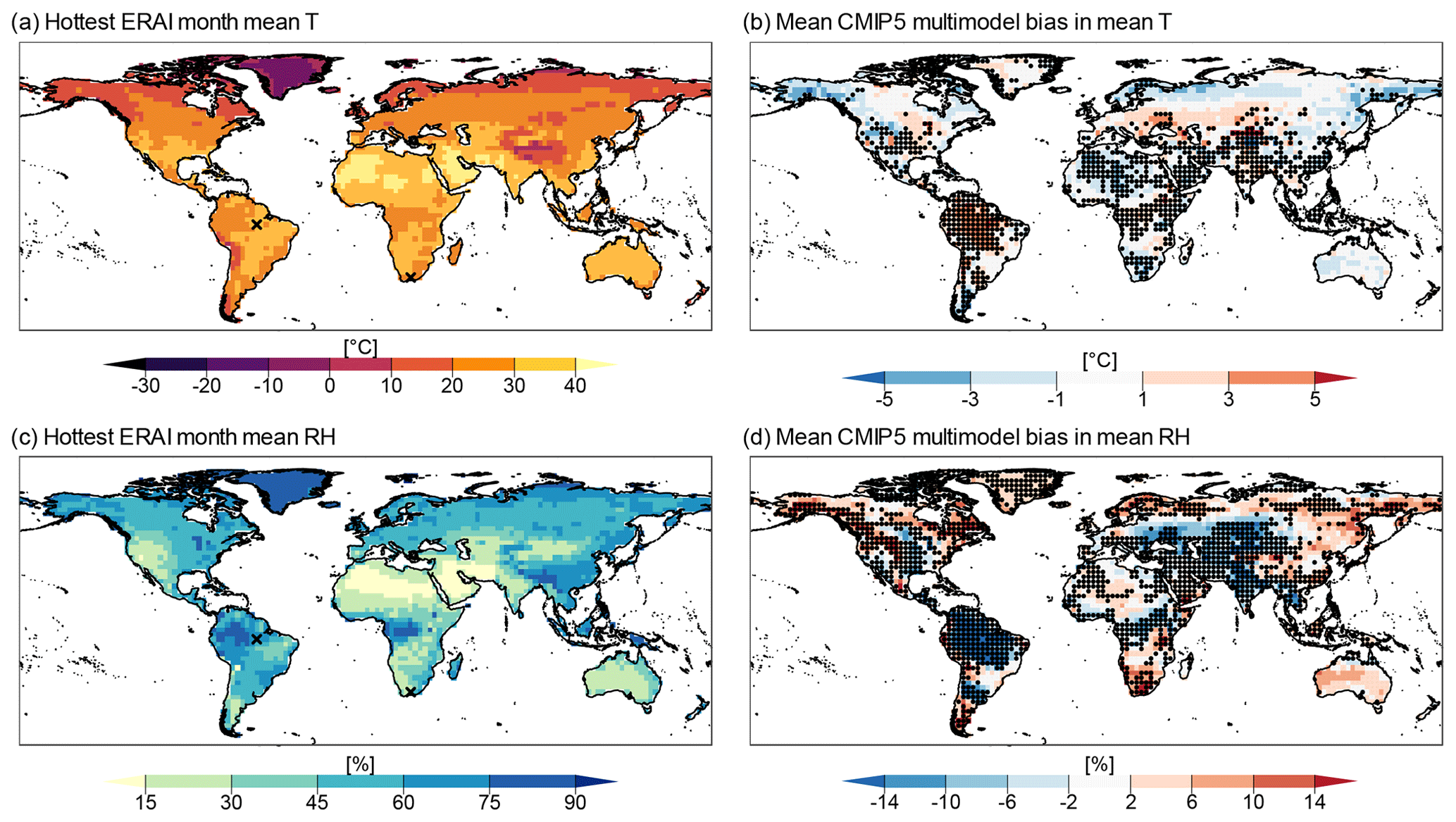
Figure 3Mean temperature (T) of the hottest month in ERA-Interim reanalysis (a), mean CMIP5 multimodel bias in mean temperature (b), mean relative humidity (RH) of ERA-Interim reanalysis (c), and mean CMIP5 multimodel bias in mean RH (d). Stippling indicates locations where at least 75 % of models failed the AD two-sample test between the CMIP5 and ERA-Interim marginal distributions of T and RH. Bias was calculated as (CMIP5 minus ERA-Interim).
4.1.2 T and RH
Following the evaluation of CBI and WBGT, we move towards evaluating how CMIP5 models represent the driving variables of the hazard indicators, i.e. T, RH, and their statistical dependence. We first confirm that the expected latitudinal variation in T is present in ERA-Interim reanalysis (Fig. 3a) and that RH is low over known desertic areas (Fig. 3c).
The spatial pattern of mean T is well represented by CMIP5 models (Fig. A3c), with all models showing a pattern correlation over land with ERA-Interim above 0.93, consistent with an acceptable representation of the first-order global-scale atmospheric circulation. However, significant differences in the representation of the distributions (based on the AD test) are found over the Amazon basin, where the multimodel mean bias in mean T is positive, and over Northern Africa and the Middle East, where the bias in mean T is negative (Fig. 3b). Overall, we found that the area-weighted multimodel mean of the absolute value of the T bias is 1.6 ∘C. The AD test results show that CMIP5 models fail to reproduce the observed ERA-Interim distribution of T over 40 % of the global land mass.
We find worse model skills in representing the RH distribution; in fact, models failed the AD test over 59 % of the global land mass (Fig. 3d). The spatial pattern of RH is not as well represented as that of T, with minimum and maximum pattern correlations of 0.75 and 0.90, respectively (Fig. A3d). The mean multimodel bias in RH is particularly large in the Amazon basin. Nevertheless, there are areas where the bias is relatively small, e.g. in Australia, the Sahara, and eastern Asia. Notably, there is a clear resemblance between the bias patterns of mean RH (Fig. 3d) and CBI (Fig. 2b), with regions with high positive bias in RH corresponding to regions with strong negative bias in CBI, and an identical percentage of land mass showing significant differences. No similar behaviour is found for WBGT; i.e. the WBGT bias spatial pattern is similar neither to that of T nor RH bias. We will investigate this behaviour in CBI and WBGT in further detail in Sect. 4.3.
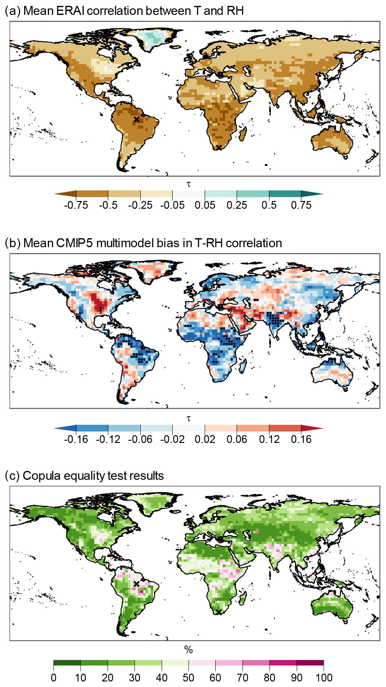
Figure 4Mean ERA-Interim correlation (τ) between T and RH (a), mean CMIP5 multimodel bias in τ (b), and the proportion of CMIP5 samples where the copula equality was rejected (c). Stippling in panel (b) indicates locations where the correlations of more than 75 % of CMIP5 model samples have significantly different values compared to ERA-Interim, as calculated using Bonferroni-corrected p values. Bias was calculated as (CMIP5 minus ERA-Interim).
4.2 Dependence between T and RH
The results for our tests on the dependency structure of T and RH in CMIP5 models are shown in Fig. 4. Figure 4a and b show Kendall's τ correlation between T and RH based on ERA-Interim reanalysis and the mean multimodel bias of this correlation, respectively. T and RH are strongly negatively correlated (Fig. 4a), with an area-weighted mean value of −0.50 (virtually all land mass has a significant correlation; not shown are results based on the indepTest function of the copula R package; v0.999–19.1; Hofert et al., 2018). The presence of a negative correlation is illustrated in Fig. 1 (and A1 for a representative location). The area-weighted absolute mean multimodel bias in τ is 0.095. The bias in τ is not significant for most of the global land mass for most of the models; i.e. the modelled correlations lie within the 95 % confidence interval of τ of ERA-Interim (see infrequent stippling over 5.3 % and 9.3 % of land masses in Figs. 4b and A4, respectively). Results are similar for the copula equality test (Fig. 4c), with an over 80 % agreement in copula structure between ERA-Interim and models for 52 % of land masses and 60 %–80 % agreement in 33 % of land masses. Overall, the regions where we detect the highest amount of statistically significant differences in the copula structure and τ include parts of the Horn of Africa, India, and the Amazon basin (see also Fig. A1c and d, where the model values have different distributions compared to ERA-Interim).
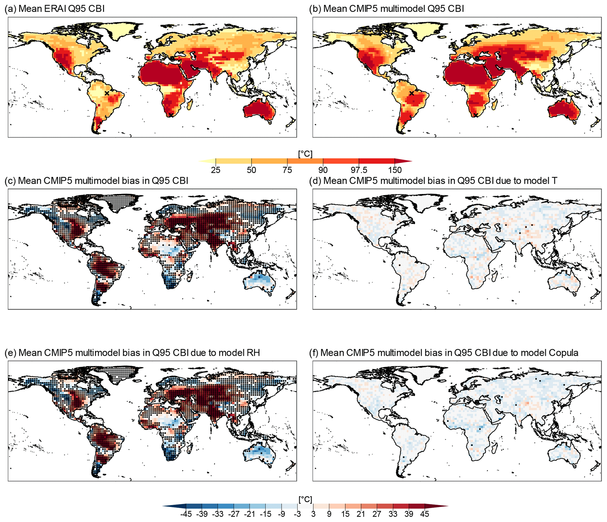
Figure 5ERA-Interim (a) and CMIP5 multimodel mean (b) 95th quantile CBI values. Note that the palette is non-linear, as it follows typical defined ranges of fire hazard levels based on the CBI, i.e. very low, low, moderate, high, very high, and extreme. Mean CMIP5 multimodel bias in Q95 CBI (c), and its decomposition into bias due to the T (d), RH (e), and copula (f) components of the models. Stippling indicates locations where more than 75 % of CMIP5 model sample values lie outside the 95 % confidence interval for ERA-Interim estimated based on bootstrap samples. Bias was calculated as (CMIP5 or transformation minus ERA-Interim).
4.3 Contribution of the bias in the drivers to the bias in CBI and WBGT extremes
4.3.1 Drivers of the biases in CBI extremes
We now assess the biases in the representation of extreme events (95th quantile, Q95) in the CBI index and the associated drivers of the biases (Fig. 5). The spatial pattern of the CMIP5 multimodel mean of Q95 (Fig. 5b) is very similar to that of ERA-Interim (Fig. 5a). Figure 5c shows the biases in extreme CBI, whose highest values are in South America, central North America, and parts of central Asia, which is in line with the biases in mean CBI (Fig. 2b). The area-weighted mean of absolute bias in the CMIP5 model CBI is 21 ∘C, which is large compared to the area-weighted mean CBI in ERA-Interim of 84 ∘C (i.e. corresponding to 25 %). In fact, the stippling over 75 % of land masses in Fig. 5c indicates that the models differ significantly from ERA-Interim.
The bias in RH is the main contributor to total mean bias in extreme CBI values (Fig. 6d–f). The relevance of RH for the bias in CBI is visible from the similarities in magnitude and spatial distribution of bias between Fig. 5c and e. Furthermore, while the area-weighted mean of absolute bias in CBI is 21 ∘C, the corresponding mean biases due to T, RH, and the dependency between them are 3, 20, and 3 ∘C, respectively. The relevant contribution of RH to the CBI index bias is consistent with the definition of the index, which is mainly influenced by RH and to a lesser extent by T (see nearly horizontal CBI isolines in Fig. 1); hence, also the dependency between T and RH plays a negligible role. As a result, while RH bias contributions drive significant biases in CBI about everywhere but in the Sahara and Australia (see stippling over 73 % of land masses in Fig. 5c), T and dependence do not drive significant biases in CBI (see near-complete absence of stippling in Fig. 5d and f).
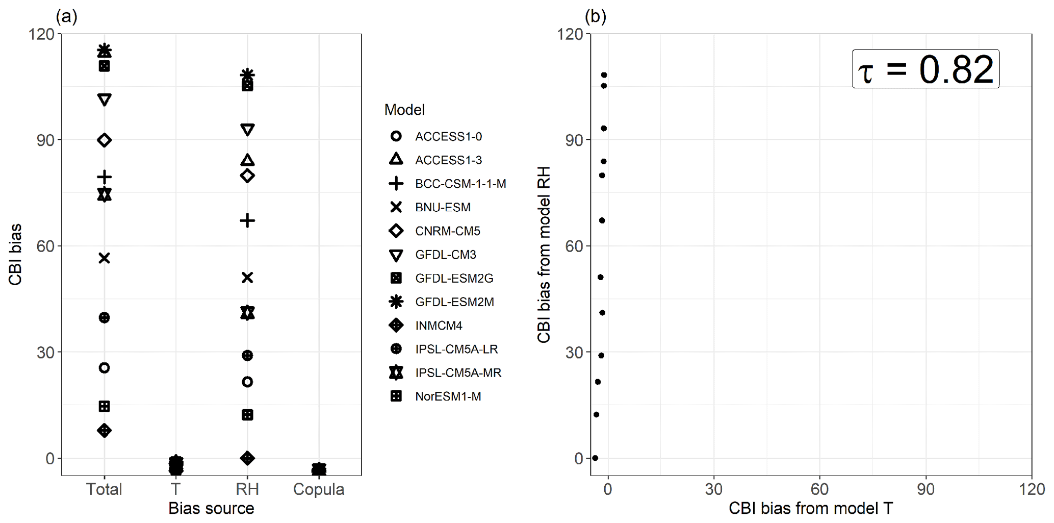
Figure 6Spread of mean total bias in the 95th quantile (Q95) of CBI and its contribution from T, RH, and their copula for individual CMIP5 models (a), and a scatter plot of the T and RH contributions to Q95 CBI bias, with their Kendall rank correlation coefficient (p value < 0.001) (b). Shown are the results for a grid point in Brazil (Amazonia, 5∘ S and 56.5∘ W). Bias was calculated as (CMIP5 or transformation minus ERA-Interim). Equal axes are used in panel (b) to highlight the differences in spread between both bias components.
A closer examination of the bias decomposition results shows, for a site with large positive bias in Brazil, that the results shown in the multimodal mean bias plots (Fig. 5c and e) reflect intermodel model behaviour at the local level. That is, CMIP5 models with high RH bias contributions also show high overall CBI bias (Fig. 6a). At this location, there is a positive intermodel correlation between the biases driven by T and RH (τ = 0.82; Fig. 6b). Such behaviour is due to the combination of the following two reasons: (1) a negative intermodel correlation between the biases in T and RH, i.e. CMIP5 models simulating temperatures that are too high also tend to simulate relative humidity that is too low (as discussed by Fischer and Knutti, 2013); and (2) the fact that CBI is high for low RH and high T. This feature is discussed in more detail in Sect. 5. Similar results to those discussed above for the site in Brazil are also observed for another representative location in South Africa with large negative bias in CBI (Fig. A5a). These locations are indicated throughout map plots with X markers.
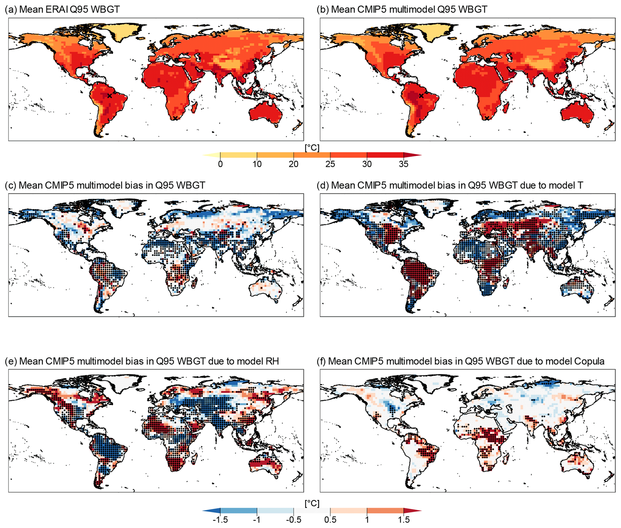
Figure 7ERA-Interim (a) and CMIP multimodel mean (b) 95th quantile WBGT values. Mean CMIP5 multimodel bias in Q95 WBGT (c) and its decomposition into bias due to the T (d), RH (e), and copula (f) components of the models. Stippling indicates locations where more than 75 % of CMIP5 model sample values lie outside the 95 % confidence interval for ERA-Interim estimated based on bootstrap samples. Bias was calculated as (CMIP5 or transformation minus ERA-Interim).
4.3.2 Drivers of the biases in WBGT extremes
The spatial pattern of Q95 in ERA-Interim (Fig. 7a) and in the CMIP5 multimodel mean (Fig. 7b) is similar, with low values concentrated along mountain ranges such as the Andes and Himalayas and in high latitudes and with the highest values located in South America and the Indian subcontinent. In several regions worldwide, CMIP5 models tend to underestimate Q95 values of WBGT (global area-weighted mean bias of −0.35 ∘C) and show significant biases relative to ERA-Interim along the tropics and subtropics (Fig. 7c). However, in terms of values of the bias, the CMIP5 representation of the WBGT appears better than that of CBI. The area-weighted mean of absolute bias in the index is 1.1 ∘C (Fig. 7c), which is small compared to the area-weighted mean WBGT in ERA-Interim, i.e. 29 ∘C (Fig. 7a).
The decomposition of the bias shows that unlike CBI there is no single dominating source of bias in extreme values of WBGT (Fig. 7d–f); all three possible sources contribute to the overall bias. Importantly, a degree of compensating biases is evident when comparing the multimodel mean biases driven by T (Fig. 7d) and RH (Fig. 7e). Large biases of opposite signs are evident over South America, central Asia, and other land masses; hence, in these areas, the resulting biases in WBGT tend to be small (Fig. 7c). Significant but opposite biases in T and RH (see stippling in Fig. 7d and e) result in nonsignificant biases in WBGT (Fig. 7c) over regions such as North America's Mississippi basin and around Zaire in central Africa. Globally, this compensating behaviour can be observed in the percentages of land masses where each bias component is significant. T- and RH-driven biases are significant over 69 % and 48 % of the global land mass, respectively, while copula biases are significant over 12 %; however, the total bias in WBGT is only significant over 39 % of land masses. Further evidence for these compensating biases can be found by observing that the area-weighted average of absolute bias in Q95 WBGT, i.e. 1.1 ∘C, is smaller than the contributions from T and RH, i.e. 1.9 and 1.4 ∘C, respectively. In addition, we observe a tendency towards a lower bias, on average, driven by the copula component (global area-weighted average of absolute bias equal to 0.85 ∘C); note that, however, some relevant positive bias contributions exist over eastern Brazil and central Africa, where the copula test shows higher frequencies of rejection (Fig. 4c), and a negative contributions over northern Russia, the central United States, and eastern Europe (Fig. 7f).
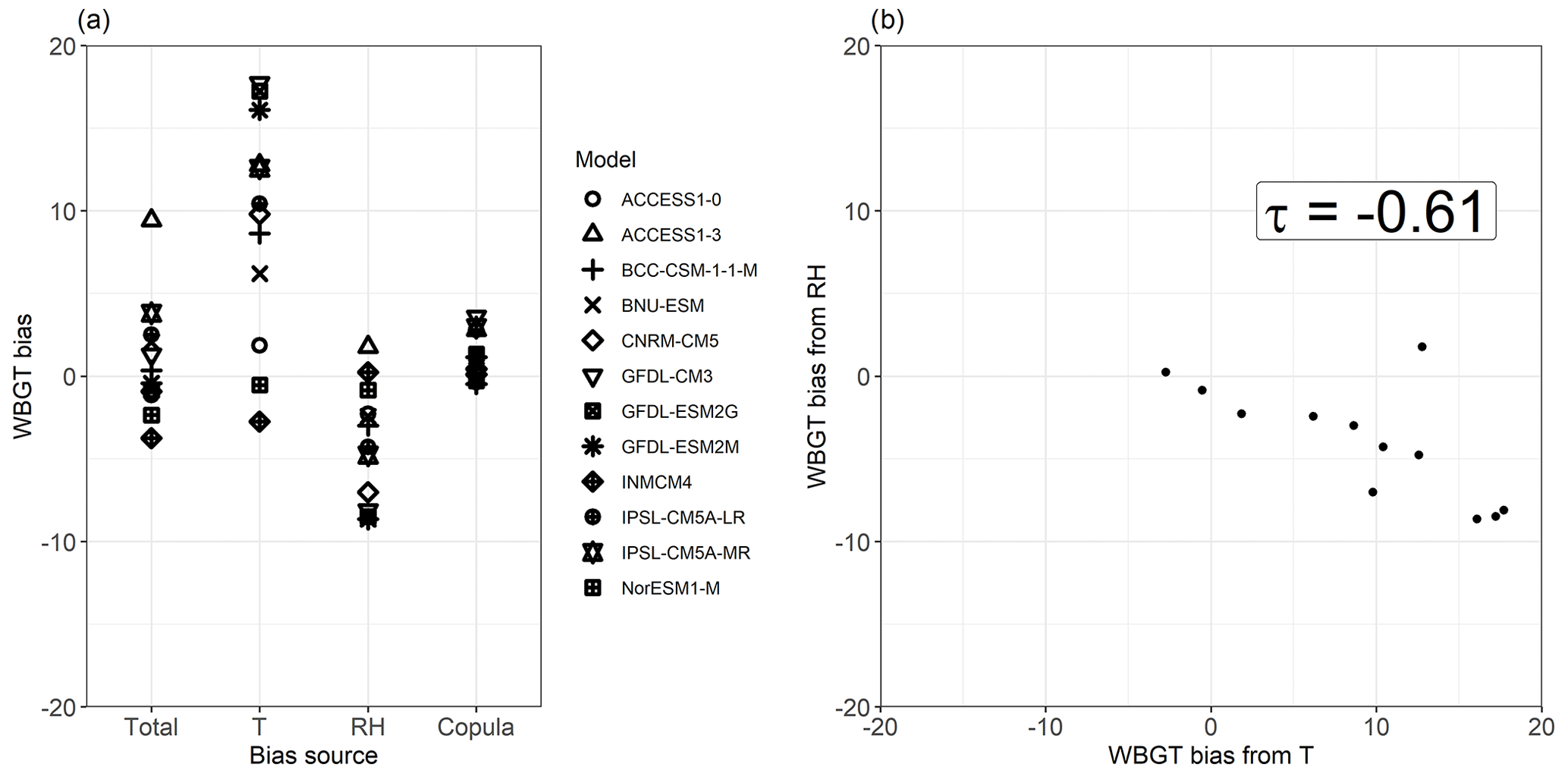
Figure 8Spread of mean total bias in the 95th quantile (Q95) of WBGT and its contribution from T, RH, and their copula for individual CMIP5 models (a), and a scatter plot of the T and RH contributions to Q95 WBGT bias, with their respective Kendall rank correlation coefficient (p value < 0.001). Shown are results for a grid point in Brazil (Amazonia, 5∘ S and 56.5∘ W). Bias was calculated as (CMIP5 or transformation minus ERA-Interim). Equal axes are used in panel (b) to highlight the differences in spread between both bias components.
The compensating bias in T and RH found above is in line with the findings of Fischer and Knutti (2013). Their results indicate that, at the local scale and for individual models, the biases in WBGT driven by T and RH tend to cancel each other out, resulting in small biases in the heat stress index. We find that this behaviour in individual models is reflected in the multimodel mean result (Fig. 7c) in regions where most models have similar behaviours, e.g. where most models show a positive WBGT bias contribution from T (Fig. 7d) and a negative one from RH (Fig. 7e). We confirm the behaviour in individual models for two representative locations. In Brazil, the small mean bias in WBGT Q95 for all CMIP5 models results from mostly positive and negative biases driven by T and RH, respectively, across models (Fig. 8a; the figure also indicates that the bias driven by the dependence is small and positive). In particular, models affected by a positive T bias contribution in WBGT because of T that is too high tend also to be affected by a negative RH bias contribution because of RH that is too low (Fig. 8b). The compensation of the biases in individual models arises from (1) opposite biases in T and RH (models simulating temperatures that are too high also tend to simulate relative humidity that is too low; Fischer and Knutti, 2013) and (2) the WBGT tendency to be high (low) for humid and warm (dry and cold) conditions. Figure A6 illustrates such a cancellation of the bias in WBGT for a location in South Africa, where the negative dependency between T and RH leads to a small bias in WBGT. In this location, the model biases driven by T are negative; therefore those driven by RH are positive.
Our results underline the importance of understanding the sources of the biases in hazard indicators through multivariate procedures. In fact, hazard indicators can have biases resulting from a complex combination of biases in the driving variables of the indicator and in biases in the dependence between the variables. We find that biases in CBI extremes are mainly driven by biases in relative humidity, while biases in WBGT extremes are often driven by biases in temperature, relative humidity, and their statistical dependence.
Biases in WBGT are smaller than the bias contributions from T and RH, i.e. the biases in the two variables compensate. In particular, in line with Fischer and Knutti (2013), models which tend to simulate T that is too high also tend to simulate RH that is too low (and vice versa), which results in relatively smaller absolute biases in the WBGT of individual models. A negative intermodel correlation between the contributions of T and RH to WBGT biases reduces the biases in WBGT in the CMIP5 average. For the fire hazard, despite that fact that a positive intermodel correlation between the bias driven by T and RH exists, no enhancement of the CBI bias occurs because the index is mainly controlled by RH (see isolines in Fig. 1c), which also controls the bias of the index. The WBGT index shows additional complexity due to the contribution of the biases in the copula between T and RH in areas such as eastern Brazil, Africa, and parts of central North America and India.
These findings exemplify the need for multivariate bias adjustment methods, which can adjust climate model biases in the dependencies between multiple drivers of hazards (Francois et al., 2020; Vrac, 2018). Furthermore, relying on climate models that plausibly represent large-scale atmospheric circulation (Maraun, 2016; Maraun et al., 2017) would improve our confidence in the simulation of multivariate hazards. The relevance of multivariate bias adjustment methods is also supported by the fact that adjusting biases variable by variable may even increase biases in impact-relevant indicators (Zscheischler et al., 2019). Nevertheless, in line with our findings, Zscheischler et al. (2019) found that univariate bias adjustment is relatively efficient in the case of CBI, while multivariate methods lead to much stronger reductions in the case of WBGT. It should be noted, however, that the considered fire indicator CBI is overly simplistic. In practice, weather conditions that promote fires are also related to wind speed and previous rainfall, which are for instance included in the Forest Fire Weather Index (FWI, Van Wagner, 1987), as well as fuel availability and aridity.
The presented bias decomposition method would potentially become even more relevant when considering more complex hazard indicators driven by more than two variables, such as the case of fire hazard as outlined above. This would require an extension of the bivariate copula framework. For example, in the case of three variables – X1, X2, and X3 – we would have to investigate the behaviour of marginals, the dependence between X1 and X2 (with the two-dimensional copula C12), X2 and X3 (C23), and X1 and X3 (C13), and then the joint behaviour of the three variables with the three-dimensional copula (C123). Alternatively, vine copula decompositions could be employed (Hobæk Haff et al., 2015). Similar considerations apply for the consideration of temporal dependencies. The analysis can be done using both a parametric or non-parametric approach. For instance, in Vezzoli et al. (2017), a non-parametric approach has been used to analyse the behaviour of the three variables precipitation, temperature, and runoff.
Given the critical importance of addressing compound/multivariate events that are often associated with extreme impacts (Leonard et al., 2014; Zscheischler et al., 2018), we assessed the bias decomposition for high quantiles of CBI and WBGT. The extremes of the considered indicators are not necessarily caused by extreme values of the drivers. Hence, the characterization of the dependence structure between their climate drivers (i.e. T and RH) was performed in terms of their full joint distribution to capture all the events; i.e. we did not only consider the combination of simultaneous T and RH extremes. However, depending on the type of hazard considered, investigating biases in the tail dependence between the drivers may be relevant to understanding the biases in the hazard. For example, the tail dependence between storm surge and precipitation, which is relevant for compound coastal flooding, may be slightly underestimated in CMIP5 models (Bevacqua et al., 2019). Similarly, there is evidence that the tail dependence between hot and dry conditions may be underestimated by climate models in some cases (Zscheischler and Fischer, 2020).
The present methodology can be used for assessing the sources of bias in other types of compound events (Zscheischler et al., 2020) caused by other sets of dependent drivers, such as compound drought and heat (Zscheischler and Seneviratne, 2017) and compound coastal flooding (Bevacqua et al., 2020b). Other types of compound events, e.g. temporal clustering of storms (Bevacqua et al. 2020c; Priestley et al., 2017) and simultaneous extreme events in distant regions (Kornhuber et al., 2020) can also lead to large impacts and are therefore relevant for the impact community. A compound-event-oriented evaluation of impacts similar to that proposed here, i.e. disentangling the biases in the individual physical drivers, could be adopted in future studies to aid present and future impact assessments.
Climate model data contain biases that need to be evaluated and ultimately adjusted to avoid misleading risk assessments. However, while many climate-related extreme impacts are caused by the combination of multiple variables, i.e. compound events, climate model evaluation methods typically do not consider the multivariate nature of the hazards. In this study, we took a compound event perspective and, based on copula theory, introduced a multivariate bias-assessment framework, which allows for disentangling and better understanding the multiple sources of biases in hazard indicators. Through a non-parametric procedure, here we investigated how the biases in temperature, relative humidity, and their dependence affect the overall biases in fire and heat stress indicators (CBI and WBGT, respectively). We found that biases in CBI are mainly driven by biases in relative humidity, in line with the fact that the index is only marginally affected by temperature. In contrast, the biases in WBGT are often driven by biases in temperature, relative humidity, and their statistical dependence (e.g. in areas including eastern Brazil, Africa, and parts of central North America and India). Opposing biases in temperature and relative humidity tend to compensate for each other, resulting in relatively small biases in WBGT. The results highlight areas where a careful interpretation of these indicators is required and where multivariate bias corrections of temperature and relative humidity should be considered future risk assessments.
Given the relevance of compound weather and climate events for societal impacts, the presented framework could be useful in further studies aiming at disentangling and better understanding the drivers of the biases in the representations of other impacts. The framework could also be useful to assess biases among drivers of hazards when data for the hazard indicators are not available. A compound-event-oriented model evaluation of modelled impacts and associated drivers would be beneficial for disaster risk reduction and, ultimately, could feed back into climate model development processes and stimulate the design of new bias adjustment methods.
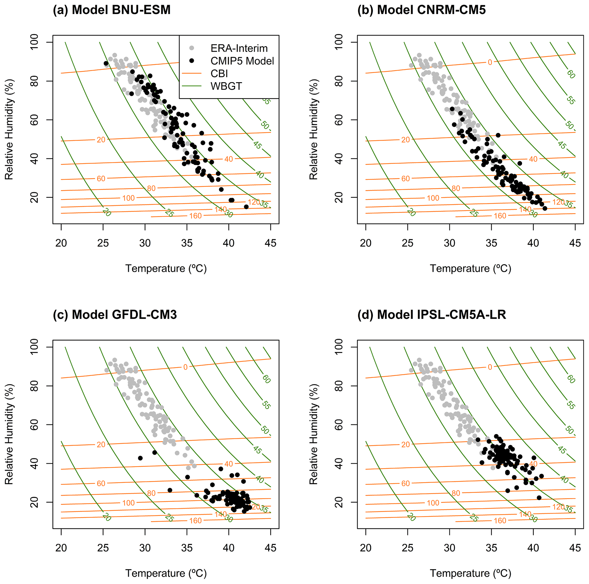
Figure A1Samples of hourly 2 m air T (∘C) vs. RH (%) during the period 1979–2005 for ERA-Interim reanalysis (grey points) and four models (black points) from the CMIP5 multimodel ensemble (BNU-ESM (a), GFDL-CM3 CNRM-CM5 (b), GFDL-CM3 (c), and IPSL-CM5A-LR (d)) for a grid point in Brazil (Amazonia, 5∘ S and 56.5∘ W) indicated throughout map plots in the Results section (Sect. 4) with X markers. The isolines illustrate equal levels of the hazard indices of fire (orange) and heat stress (green), corresponding to CBI and WBGT indices, respectively, which are both functions of T and RH.
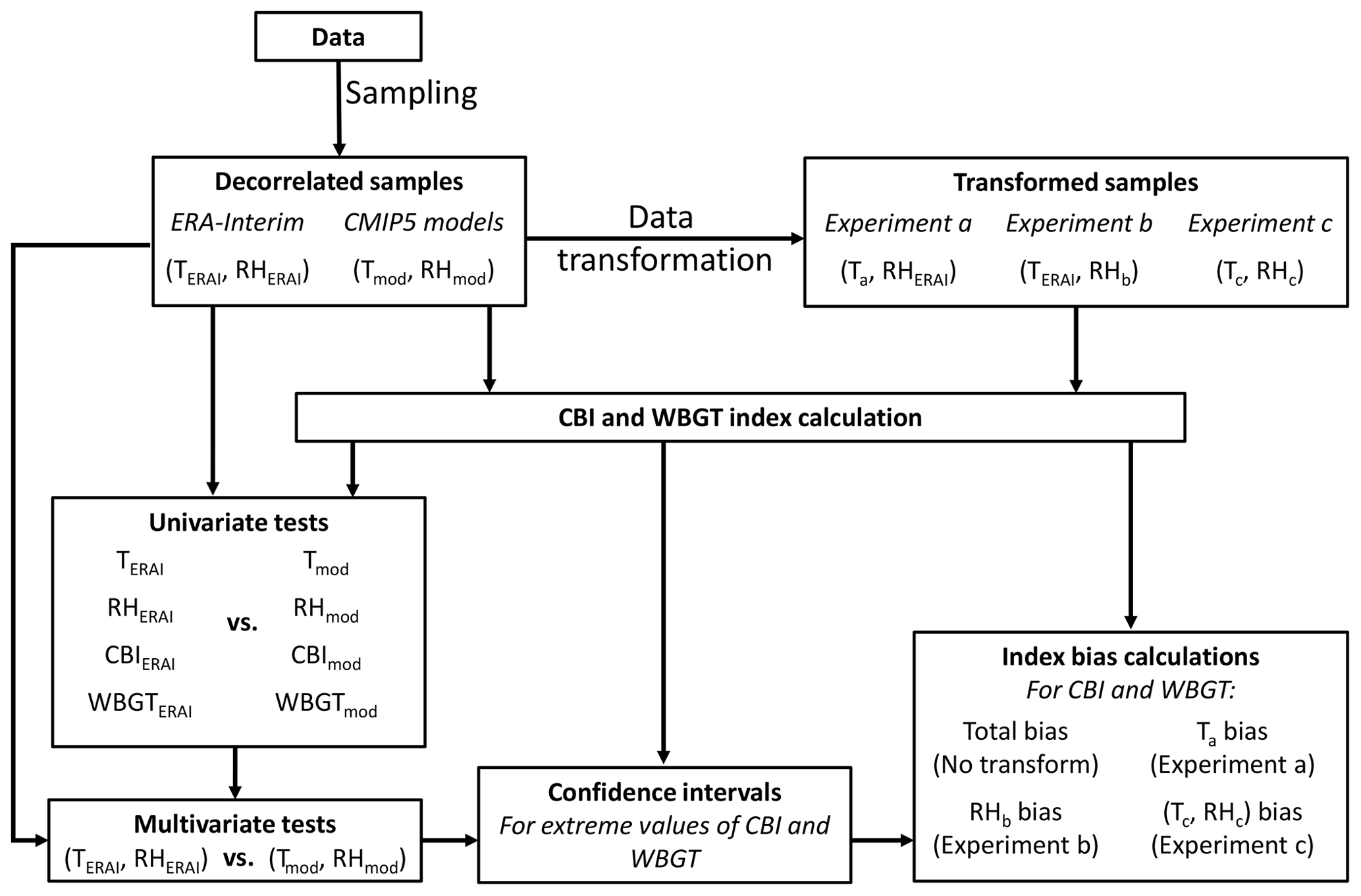
Figure A2Block diagram showing the data and methods used. Temperature (T) and relative humidity (RH) decorrelated samples from CMIP5 models' biases are analysed using univariate and multivariate statistical tests using ERA-Interim as reference dataset. We also create transformed CMIP5 model samples, which allow for assessing the bias in the extreme values of the hazard indicator (CBI and WBGT) driven by biases in T, RH, and their statistical dependence.
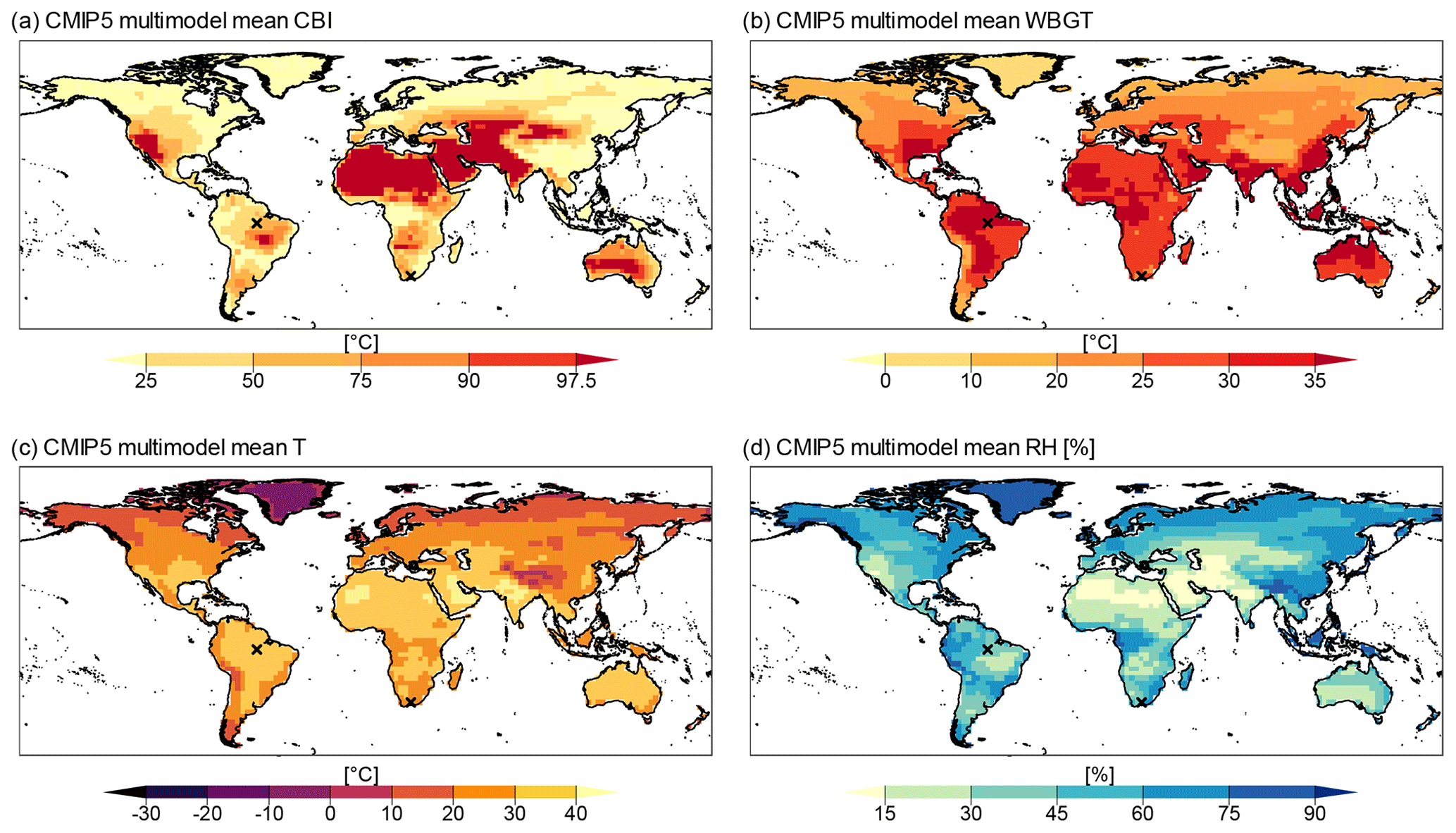
Figure A3CMIP5 multimodel mean fire hazard index (CBI) value (a), heat stress index (WBGT) value (b), temperature (T) value (c), and relative humidity (RH) (d).
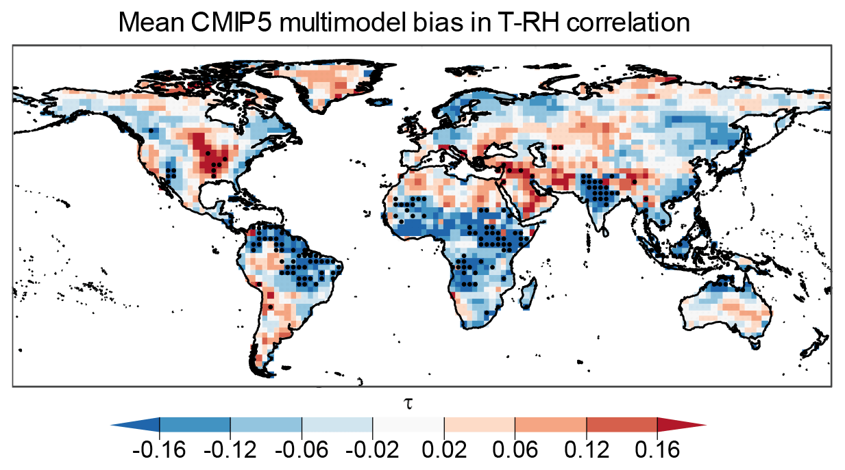
Figure A4As Fig. 4b but where stippling indicates locations where more than 75 % of CMIP5 model sample values lie outside the 95 % confidence interval for ERA-Interim.
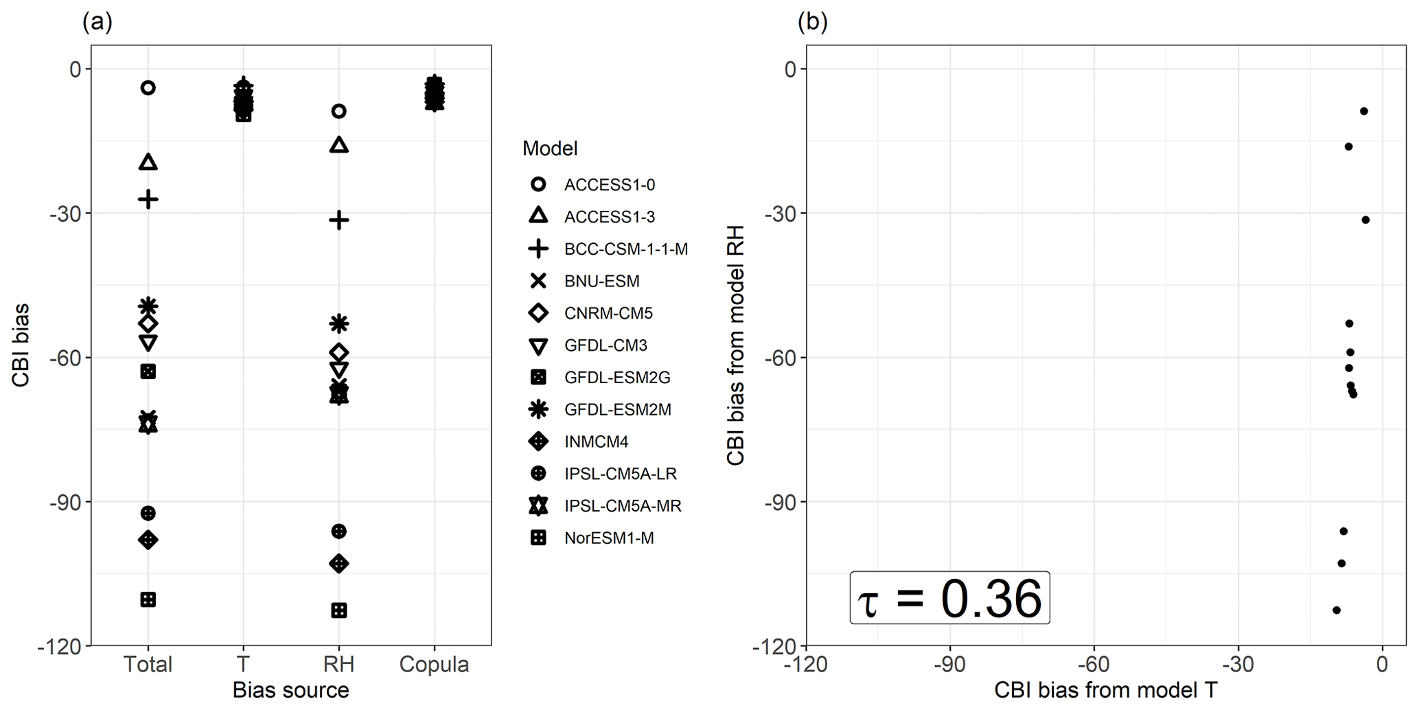
Figure A5As Fig. 6 for a grid point in South Africa (32.5∘ S and 23.5∘ E), with Kendall rank correlation p value = 0.12.
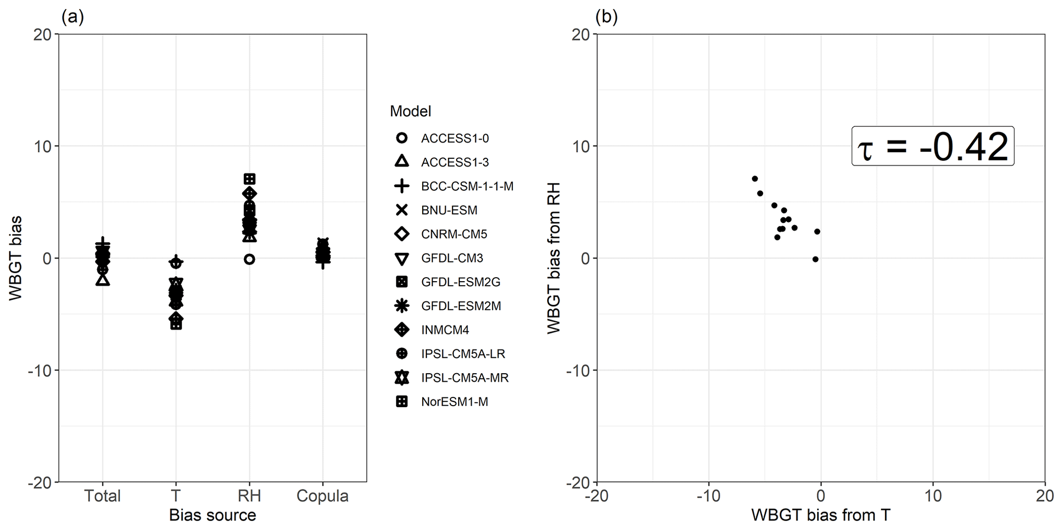
Figure A6As Fig. 8 for a grid point in South Africa (32.5∘ S and 23.5∘ E), with Kendall rank correlation p value = 0.063.
Data from CMIP5 models are available from the Earth System Grid Federation (ESGF) peer-to-peer system (https://esgf-node.llnl.gov/projects/cmip5, last access: June 2021) (WCRP, 2021). The ERA-Interim reanalysis dataset is available from the ECMWF Public Datasets web page (https://apps.ecmwf.int/datasets/, last access: June 2021) (ECMWF, 2021).
EB and CDM conceived the study and supervised the project. RVH carried out the analysis of the biases based on the data prepared by EB, AFSR, LC, GA, BM, and MH. RVH prepared all the figures except Figs. 1 and A1, which were prepared by EB and AR. The paper was written by GA, EB, CDM, AR, and RVH. JZ contributed to the development of the idea of the work and helped with final edits. All the authors discussed the results of the paper.
The authors declare that they have no conflict of interest.
This article is part of the special issue “Understanding compound weather and climate events and related impacts (BG/ESD/HESS/NHESS inter-journal SI)”. It is not associated with a conference.
This work emerged from the Training School on Statistical Modelling Compound Events organized by the European COST Action DAMOCLES (CA17109). We acknowledge the World Climate Research Programme Working Group on Coupled Modelling, which is responsible for CMIP, and we thank the climate modelling groups for producing and making available their model output.
Emanuele Bevacqua was supported by the European Research Council grant ACRCC (project 339390) and the DOCILE project (NERC grant NE/P002099/1). Andreia F. S. Ribeiro was supported by the Portuguese Foundation for Science and Technology (FCT) (grant PD/BD/114481/2016), the project IMPECAF (PTDC/CTA-CLI/28902/2017), and the Swiss National Science Foundation (project number 186282). Carlo De Michele was supported by the Italian Ministry of Education, University and Research through the PRIN2017 RELAID project. The work of Laura Crocetti was supported by the TU Wien Wissenschaftspreis 2015, awarded to Wouter Dorigo. Roberto Villalobos-Herrera was supported by the University of Costa Rica and the Newcastle University School of Engineering. Jakob Zscheischler was supported by the Swiss National Science Foundation (Ambizione grant 179876) and the Helmholtz Initiative and Networking Fund (Young Investigator Group COMPOUNDX, grant agreement VH-NG-1537).
This paper was edited by Ricardo Trigo and reviewed by Mathieu Vrac and one anonymous referee.
ASCM – American College of Sports Medicine: Prevention of Thermal Injuries During Distance Running – Position stand, Med. Sci. Sport. Exerc., 16, ix–xiv, 1984.
Berrisford, P., Kållberg, P., Kobayashi, S., Dee, D., Uppala, S., Simmons, A. J., Poli, P., and Sato, H.: Atmospheric conservation properties in ERA-Interim, Q. J. Roy. Meteor. Soc., 137, 1381–1399, https://doi.org/10.1002/qj.864, 2011.
Bevacqua, E., Maraun, D., Hobæk Haff, I., Widmann, M., and Vrac, M.: Multivariate statistical modelling of compound events via pair-copula constructions: analysis of floods in Ravenna (Italy), Hydrol. Earth Syst. Sci., 21, 2701–2723, https://doi.org/10.5194/hess-21-2701-2017, 2017.
Bevacqua, E., Maraun, D., Vousdoukas, M. I., Voukouvalas, E., Vrac, M., Mentaschi, L., and Widmann, M.: Higher probability of compound flooding from precipitation and storm surge in Europe under anthropogenic climate change, Science Advances, 5, 9, eaaw5531, https://doi.org/10.1126/sciadv.aaw5531, 2019.
Bevacqua, E., Vousdoukas, M. I., Shepherd, T. G., and Vrac, M.: Brief communication: The role of using precipitation or river discharge data when assessing global coastal compound flooding, Nat. Hazards Earth Syst. Sci., 20, 1765–1782, https://doi.org/10.5194/nhess-20-1765-2020, 2020a.
Bevacqua, E., Vousdoukas, M. I., Zappa, G., Hodges, K., Shepherd, T. G., Maraun, D., Mentaschi, L., and Feyen, L.: More meteorological events that drive compound coastal flooding are projected under climate change, Commun. Earth Environ., 1, 47, https://doi.org/10.1038/s43247-020-00044-z, 2020b.
Bevacqua, E., Zappa, G., and Shepherd, T. G.: Shorter cyclone clusters modulate changes in European wintertime precipitation extremes, Environ. Res. Lett., 15, 124005, https://doi.org/10.1088/1748-9326/abbde7, 2020c.
Brando, P. M., Balch, J. K., Nepstad, D. C., Morton, D. C., Putz, F. E., Coe, M. T., Silvério, D., Macedo, M. N., Davidson, E. A., Nóbrega, C. C., Alencar, A., and Soares-Filho, B. S.: Abrupt increases in Amazonian tree mortality due to drought-fire interactions, P. Natl. Acad. Sci. USA, 111, 6347–6352, https://doi.org/10.1073/pnas.1305499111, 2014.
Dale, M. and Fortin, M.: Spatial Autocorrelation and Statistical Tests: Some Solutions, J. Agr. Biol. Envir. St., 14, 188–206, 2009.
Dee, D. P., Uppala, S. M., Simmons, A. J., Berrisford, P., Poli, P., Kobayashi, S., Andrae, U., Balmaseda, M. A., Balsamo, G., Bauer, P., Bechtold, P., Beljaars, A. C. M., van de Berg, L., Bidlot, J., Bormann, N., Delsol, C., Dragani, R., Fuentes, M., Geer, A. J., Haimberger, L., Healy, S. B., Hersbach, H., Hólm, E. V., Isaksen, L., Kållberg, P., Köhler, M., Matricardi, M., McNally, A. P., Monge-Sanz, B. M., Morcrette, J.-J., Park, B.-K., Peubey, C., de Rosnay, P., Tavolato, C., Thépaut, J.-N., and Vitart, F.: The ERA-Interim reanalysis: configuration and performance of the data assimilation system, Q. J. Roy. Meteor. Soc., 137, 553–597, https://doi.org/10.1002/qj.828, 2011.
Durante, F. and Sempi, C.: Principles of Copula Theory, 1st Edn., Chapman and Hall/CRC, https://doi.org/10.1201/b18674, 2015.
ECMWF: Public Datasets, available at: https://apps.ecmwf.int/datasets/, last access: June 2021.
FIALA, D., Havenith, G., Bröde, P., Kampmann, B., and Jendritzky, G.: UTCI-Fiala multi-node model of human heat transfer and temperature regulation, Int. J. Biometeorol., Special Issue, 1–13, 2011.
Fischer, E. M. and Knutti, R.: Robust projections of combined humidity and temperature extremes, Nat. Clim. Change, 3, 126–130, https://doi.org/10.1038/nclimate1682, 2013.
François, B., Vrac, M., Cannon, A. J., Robin, Y., and Allard, D.: Multivariate bias corrections of climate simulations: which benefits for which losses?, Earth Syst. Dynam., 11, 537–562, https://doi.org/10.5194/esd-11-537-2020, 2020.
Hobæk Haff, I., Frigessi, A., and Maraun, D.: How well do regional climate models simulate the spatial dependence of precipitation? An application of pair-copula constructions, J. Geophys. Res.-Atmos., 120, 2624–2646, https://doi.org/10.1002/2014JD022748, 2015.
Hofert, M., Kojadinovic, I., Maechler, M., and Yan, J.: copula: Multivariate Dependence with Copulas, R package version 0.999-19.1, available at: https://CRAN.R-project.org/package=copula (last access: 19 November 2020), 2018.
Hollander, M., Wolfe, D. A., and Chicken, E.: Nonparametric Statistical Methods, 3rd Edn., John Wiley & Sons, Hoboken, New Jersey, 2014.
Jafari, M. and Ansari-Pour, N.: Why, When and How to Adjust Your P Values?, Cell J., 20, 604–607, https://doi.org/10.22074/cellj.2019.5992, 2019.
Jézéquel, A., Bevacqua, E., D'Andrea, F., Thao, S., Vautard, R., Vrac, M., and Yiou, P.: Conditional and residual trends of singular hot days in Europe, Environ. Res. Lett., 15, 064018, https://doi.org/10.1088/1748-9326/ab76dd, 2020.
Kornhuber, K., Coumou, D., Vogel, E., Lesk, C., Donges, J. F., Lehmann, J., and Horton, R. M.: Amplified Rossby waves enhance risk of concurrent heatwaves in major breadbasket regions, Nat. Clim. Change, 10, 48–53, 2020.
Leonard, M., Westra, S., Phatak, A., Lambert, M., van den Hurk, B., Mcinnes, K., Risbey, J., Schuster, S., Jakob, D., and Stafford-Smith, M.: A compound event framework for understanding extreme impacts, WIREs Clim. Change, 5, 113–128, https://doi.org/10.1002/wcc.252, 2014.
Manning, C., Widmann, M., Bevacqua, E., Van Loon, A. F., Maraun, D., and Vrac, M.: Soil moisture drought in Europe: a compound event of precipitation and potential evapotranspiration on multiple timescales, J. Hydrometeorol., 19, 1255–1271, https://doi.org/10.1175/JHM-D-18-0017.1, 2018.
Manning, C., Widmann, M., Bevacqua, E., Van Loon, A. F., Maraun, D., and Vrac, M.: Increased probability of compound long-duration dry and hot events in Europe during summer (1950–2013), Environ. Res. Lett., 14, 094006, https://doi.org/10.1088/1748-9326/ab23bf, 2019.
Maraun, D.: Bias Correcting Climate Change Simulations – a Critical Review, Current Climate Change Reports, 2, 211–220, https://doi.org/10.1007/s40641-016-0050-x, 2016.
Maraun, D., Shepherd, T. G., Widmann, M., Zappa, G., Walton, D., Gutiérrez, J. M., Hagemann, S., Richter, I., Soares, P. M. M., Hall, A., and Mearns, L. O.: Towards process-informed bias correction of climate change simulations, Nat. Clim. Change, 7, 764–773, https://doi.org/10.1038/nclimate3418, 2017.
McCutchan, M. H. and Main, W. A.: The relationship between mean monthly fire potential indices and monthly fire severity, in: Proceedings of the 10th Conference on Fire and Forest Meteorology, edited by: MacIver, D. C., Auld, H., and Whitewood, R., Forestry Canada, Ottawa, Ontario, Canada, 430–435, 1989.
Nelsen, R. B.: An Introduction to Copulas, in: Springer Series in Statistics, 2nd Edn., XIV, 272, Springer, New York, NY, https://doi.org/10.1007/0-387-28678-0, 2006.
Pfahl, S., O'Gorman, P., and Fischer, E.: Understanding the regional pattern of projected future changes in extreme precipitation, Nat. Clim. Change, 7, 423–427, https://doi.org/10.1038/nclimate3287, 2017.
Priestley, M. D., Pinto, J. G., Dacre, H. F., and Shaffrey, L. C.: The role of cyclone clustering during the stormy winter of 2013/2014, Weather, 72, 187–192, 2017.
Raymond, C., Matthews, T., and Horton, R. M.: The emergence of heat and humidity too severe for human tolerance, Science Advances, 6, eaaw1838, https://doi.org/10.1126/sciadv.aaw1838, 2020.
R Core Team: R: A language and environment for statistical computing, R Foundation for Statistical Computing, Vienna, Austria, available at: https://www.R-project.org/ (last access: 19 November 2020), 2019.
Remillard, B. and Plante, J.-F.: TwoCop: Nonparametric test of equality between two copulas, R package version 1.0, available at: https://CRAN.R-project.org/package=TwoCop (last access: 19 November 2020), 2012.
Rémillard, B. and Scaillet, O.: Testing for equality between two copulas, J. Multivariate Anal., 100, 377–386, https://doi.org/10.1016/j.jmva.2008.05.004, 2009.
Roads, J. P., Tripp, P., Juang, H., Wang, J., Chen, S., and Fujioka, F.: ECPC/NCEP March 2008 seasonal fire danger forecasts, in: Experimental Long-Lead Forecasts Bulletin, 17, National Centers for Environmental Prediction, Camp Springs, Maryland, 7 pp., 2008.
Russo, S., Sillmann, J., and Sterl, A.: Humid heat waves at different warming levels, Sci. Rep., 7, 1–7. https://doi.org/10.1038/s41598-017-07536-7, 2017.
Salvadori, G. and De Michele, C.: On the Use of Copulas in Hydrology: Theory and Practice, J. Hydrol. Eng., 12, 369–380, https://doi.org/10.1061/(ASCE)1084-0699(2007)12:4(369), 2007.
Salvadori, G., De Michele, C., Kottegoda, N. T., and Rosso, R.: Extreme in nature: An approach using copulas, Springer, Dordrecht, 2007.
Schär, C.: Climate extremes: The worst heat waves to come, Nat. Clim. Change, 6, 128–129, https://doi.org/10.1038/nclimate2864, 2016.
Schneider, G., Chicken, E., and Becvarik, R.: NSM3: Functions and Datasets to Accompany Hollander, Wolfe, and Chicken – Nonparametric Statistical Methods, third edn., R package version 1.15, available at: https://CRAN.R-project.org/package=NSM3 (last access: 19 November 2020), 2020.
Scholz, F. and Zhu, A.: kSamples: K-Sample Rank Tests and their Combinations, R package version 1.2-9, available at: https://CRAN.R-project.org/package=kSamples (last access: 19 November 2020), 2019.
Sklar, A.: Fonctions de Répartition à n Dimensions et Leurs Marges, Publications de l'Institut Statistique de l'Université de Paris, Paris, 8, 229–231, 1959.
Taylor, K. E., Stouffer, R. J., and Meehl, G. A.: An Overview of CMIP5 and the experiment design, B. Am. Meteorol. Soc., 93, 485–498, https://doi.org/10.1175/BAMS-D-11-00094.1, 2012.
Van Wagner, C. E.: Development and structure of the canadian forest fire weather index system, Technical Report 35, Can. Forestry Serv., Ottawa, Ontario, 48, 1987.
Vezzoli, R., Salvadori, G., and De Michele, C.: A distributional multivariate approach for assessing performance of climate-hydrology models, Sci. Rep., 7, 1–15, https://doi.org/10.1038/s41598-017-12343-1, 2017.
Vrac, M.: Multivariate bias adjustment of high-dimensional climate simulations: the Rank Resampling for Distributions and Dependences (R2D2) bias correction, Hydrol. Earth Syst. Sci., 22, 3175–3196, https://doi.org/10.5194/hess-22-3175-2018, 2018.
WCRP: Coupled Model Intercomparison Project 5 (CMIP5), available at: https://esgf-node.llnl.gov/projects/cmip5, last access: June 2021.
Yue, S., Pilon, P., Phinney, B., and Cavadias, G.: The influence of autocorrelation on the ability to detect trend in hydrological series, Hydrol. Process., 16, 1807–1829, https://doi.org/10.1002/hyp.1095, 2002.
Zscheischler, J. and Fischer, E. M.: The record-breaking compound hot and dry 2018 growing season in Germany, Weather and Climate Extremes, 29, 100270, https://doi.org/10.1016/j.wace.2020.100270, 2020.
Zscheischler, J. and Seneviratne, S. I.: Dependence of drivers affects risks associated with compound events, Science Advances, 3, 1–11, https://doi.org/10.1126/sciadv.1700263, 2017.
Zscheischler, J., Westra, S., Van Den Hurk, B. J. J. M., Seneviratne, S. I., Ward, P. J., Pitman, A., Aghakouchak, A., Bresch, D. N., Leonard, M., Wahl, T., and Zhang, X.: Future climate risk from compound events, Nat. Clim. Change, 8, 469–477, https://doi.org/10.1038/s41558-018-0156-3, 2018.
Zscheischler, J., Fischer, E. M., and Lange, S.: The effect of univariate bias adjustment on multivariate hazard estimates, Earth Syst. Dynam., 10, 31–43, https://doi.org/10.5194/esd-10-31-2019, 2019.
Zscheischler, J., Martius, O., Westra, S., Bevacqua, E., R., C., Horton, R. M., van den Hurk, B., AghaKouchak, A., Jézéquel, A., Mahecha, M. D., Maraun, D., Ramos, A. M., Ridder, N., Thiery, W., and Vignotto, E.: A typology of compound weather and climate events, Nature Reviews Earth & Environment, 1, 333–347, https://doi.org/10.1038/s43017-020-0060-z, 2020.
Zscheischler, J., Naveau, P., Martius, O., Engelke, S., and Raible, C. C.: Evaluating the dependence structure of compound precipitation and wind speed extremes, Earth Syst. Dynam., 12, 1–16, https://doi.org/10.5194/esd-12-1-2021, 2021.