the Creative Commons Attribution 4.0 License.
the Creative Commons Attribution 4.0 License.
 | 02 Jun 2021
Assessing climate-change-induced flood risk in the Conasauga River watershed: an application of ensemble hydrodynamic inundation modeling
Tigstu T. Dullo
George K. Darkwah
Sudershan Gangrade
Mario Morales-Hernández
M. Bulbul Sharif
Alfred J. Kalyanapu
Shih-Chieh Kao
Sheikh Ghafoor
Moetasim Ashfaq
This study evaluates the impact of potential future climate change on flood regimes, floodplain protection, and electricity infrastructures across the Conasauga River watershed in the southeastern United States through ensemble hydrodynamic inundation modeling. The ensemble streamflow scenarios were simulated by the Distributed Hydrology Soil Vegetation Model (DHSVM) driven by (1) 1981–2012 Daymet meteorological observations and (2) 11 sets of downscaled global climate models (GCMs) during the 1966–2005 historical and 2011–2050 future periods. Surface inundation was simulated using a GPU-accelerated Two-dimensional Runoff Inundation Toolkit for Operational Needs (TRITON) hydrodynamic model. A total of 9 out of the 11 GCMs exhibit an increase in the mean ensemble flood inundation areas. Moreover, at the 1 % annual exceedance probability level, the flood inundation frequency curves indicate a ∼ 16 km2 increase in floodplain area. The assessment also shows that even after flood-proofing, four of the substations could still be affected in the projected future period. The increase in floodplain area and substation vulnerability highlights the need to account for climate change in floodplain management. Overall, this study provides a proof-of-concept demonstration of how the computationally intensive hydrodynamic inundation modeling can be used to enhance flood frequency maps and vulnerability assessment under the changing climatic conditions.
- Article
(19553 KB) - Full-text XML
- BibTeX
- EndNote


This paper has been authored by UT-Battelle, LLC, under contract DE-AC05-00OR22725 with the US Department of Energy (DOE). The US government retains and the publisher, by accepting the article for publication, acknowledges that the US government retains a nonexclusive, paid-up, irrevocable, worldwide license to publish or reproduce the published form of this paper, or allow others to do so, for US government purposes. DOE will provide public access to these results of federally sponsored research in accordance with the DOE Public Access Plan (http://energy.gov/downloads/doe-public-access-plan).
Floods are costly disasters that affect more people than any other natural hazard around the world (UNISDR, 2015). Major factors that can exacerbate flood damage include population growth, urbanization, and climate change (Birhanu et al., 2016; Winsemius et al., 2016; Alfieri et al., 2017, 2018; Kefi et al., 2018). Recent observations exhibit an increase in the frequency and the intensity of extreme precipitation events (Pachauri and Meyer, 2014), which have strengthened the magnitude and frequency of flooding (Milly et al., 2002; Langerwisch et al., 2013; Alfieri et al., 2015a, 2018; Mora et al., 2018). As a result, the damage and cost of flooding have substantially increased across the United States (US) (Pielke and Downton, 2000; Pielke et al., 2002; Ntelekos et al., 2010; Wing et al., 2018) and the rest of the world (Hirabayashi et al., 2013; Arnell and Gosling, 2014; Alfieri et al., 2015b, 2017; Kefi et al., 2018).
Since 1968, the National Flood Insurance Program (NFIP), administered by the Federal Emergency Management Agency (FEMA), has implemented floodplain regulation standards in the US to mitigate the escalating flood losses (Bedient et al., 2013). For communities participating in the NFIP, flood insurance is required for structures located within the 1 % annual exceedance probability (AEP) flood zone (i.e., areas with probability of flooding ≥ 1 % in any given year; FEMA, 2002). However, existing floodplain protection standards have proven to be inadequate (Galloway et al., 2006; Ntelekos et al., 2010; Tan, 2013; Blessing et al., 2017; HCFCD, 2018), and climate change can likely exacerbate these issues (Olsen, 2006; Ntelekos et al., 2010; Kollat et al., 2012; AECOM, 2013; Wobus et al., 2017; Nyaupane et al., 2018; Pralle, 2019). For instance, the streamflow AEP thresholds and synthetic hydrographs used to simulate the flood zones were derived purely based on historic observations that may underestimate the intensified hydrologic extremes in the projected future climatic conditions. Although the possible change of future streamflow AEP thresholds may be evaluated by an ensemble of hydrologic model outputs driven by multiple downscaled and bias-corrected climate models (e.g., Wobus et al., 2017), the extension from maximum streamflow to maximum flood zone is not trivial and cannot be explicitly addressed through the conventional deterministic inundation modeling approach.
The increases in the magnitude and frequency of flooding, in addition to the inadequacy of floodplain measures and the high costs of hardening (Wilbanks et al., 2008; Farber-DeAnda et al., 2010; Gilstrap et al., 2015), have put electricity infrastructures at risk (Zamuda et al., 2015; Zamuda and Lippert, 2016; Cronin et al., 2018; Forzieri et al., 2018; Mikellidou et al., 2018; Allen-Dumas et al., 2019). In particular, electricity infrastructures which lie in areas vulnerable to flooding can experience floodwater damages that may lead to changes in their energy production and consumption (Chandramowli and Felder, 2014; Ciscar and Dowling, 2014; Bollinger and Dijkema, 2016; Gangrade et al., 2019). For instance, flooding can rust metals, destroy insulation, and damage interruption capacity (Farber-DeAnda et al., 2010; Vale, 2014; NERC, 2018; Bragatto et al., 2019). It is estimated that nearly 300 energy facilities are located on low-lying lands vulnerable to sea-level rise and flooding in the lower 48 US states (Strauss and Ziemlinski, 2012).
Several studies have assessed the vulnerability of electricity infrastructures to flooding (Reed et al., 2009; Winkler et al., 2010; Bollinger and Dijkema, 2016; Fu et al., 2017; Pant et al., 2017; Bragatto et al., 2019; Gangrade et al., 2019). For highly sensitive water infrastructures such as dams (McCuen, 2005), Gangrade et al. (2019) showed that the surface inundation associated with probable maximum flood (PMF) is generally projected to increase in future climate conditions. However, given the extremely large magnitude of PMF (AEP < 10−4 %), the findings cannot be directly associated with more frequent and moderate flood events (i.e., AEP around 1 %–0.2 %) that are the main focus of many engineering applications. Although some of these studies focused on evaluating the resilience of electricity infrastructures against flood hazard and/or climate change, only a few of them evaluated site-specific inundation risk and quantified impacts of climate-change-induced flooding on electricity infrastructures under different future climate scenarios. Again, one main challenge is associated with the high computational costs to effectively transform ensemble streamflow projections into ensemble surface inundation projections through hydrodynamic models. With the enhanced inundation models and high-performance computing (HPC) capabilities (Morales-Hernández et al., 2020), this challenge can be gradually overcome for more spatially explicit flood vulnerability assessment.
The objective of this study is to demonstrate the applicability of a computationally intensive ensemble inundation modeling approach to better understand how climate change may affect flood regimes, floodplain regulation standards, and the vulnerability of existing infrastructures. Extending from the framework developed by Gangrade et al. (2019) for PMF-scale events (AEP < 10−4 %) based on one selected climate model (CCSM4), we focus on more frequent extreme streamflow events (i.e., AEP around 1 %–0.2 %), which requires different modeling strategies based on multiple downscaled climate models. The unique aspects of this study are the application of an integrated climate–hydrologic–hydraulic modeling framework for the following.
-
The framework will evaluate the changes in flood regime using high-resolution ensemble flood inundation maps. The ensemble-based approach is able to incorporate the large hydrologic interannual variability and model uncertainty that cannot be captured through the conventional deterministic flood map.
-
The framework will enable direct frequency analysis of ensemble flood inundation maps that correspond to historic and projected future climate conditions. This approach provides an alternative floodplain delineation technique to the conventional approach, in which a single deterministic design flood value is used to develop a flood map with a given exceedance probability.
-
The framework will evaluate the vulnerability of electricity infrastructures to climate-change-induced flooding and assess the adequacy of existing flood protection measures using ensemble flood inundation. This information will help floodplain managers to identify the most vulnerable infrastructures and recommend suitable adaptation measures.
The following technique was adopted in this study. First, we generated streamflow projection by utilizing an ensemble of simulated streamflow hydrographs driven by both historical observations and downscaled climate projections (Gangrade et al., 2020) as inputs for hydrodynamic inundation modeling as presented in Sect. 2.2. Then, we set up and calibrated a 2D hydrodynamic inundation model, Two-dimensional Runoff Inundation Toolkit for Operational Needs (TRITON; Morales-Hernández et al., 2021), in our study area which is presented in Sect. 2.3. For inundation modeling, sensitivity analyses were conducted on three selected parameters to quantify and compare their respective influences on modeled flood depths and extents. The performance of TRITON was then evaluated by comparing a simulated 1 % AEP flood map with the reference 1 % AEP flood map from the Federal Emergency Management Agency (FEMA). Finally, as presented in Sect. 2.4 and 2.5, ensemble inundation modeling was performed to develop flood inundation frequency curves and maps and to assess the vulnerability of electricity infrastructures under a changing climate, respectively.
The article is organized as follows: the data and methods are discussed in Sect. 2; Sect. 3 presents the result and discussion; and the summary is presented in Sect. 4.
2.1 Study area
Our study area is the Conasauga River watershed (CRW) located in southeastern Tennessee and northwestern Georgia (Fig. 1). The CRW is an eight-digit Hydrologic Unit Code (HUC08) subbasin (03150101) with a total drainage area of ∼ 1880 km2. The northeastern portions of the watershed are rugged, mountainous areas largely covered with forests (Ivey and Evans, 2000; Elliott and Vose, 2005). The CRW, which is one headwater basin of the Alabama–Coosa–Tallapoosa (ACT) River basin, rises high on the Blue Ridge Mountains of Georgia and Tennessee and flows for 145 km before joining the Coosawattee River to form the Oostanaula River (Ivey and Evans, 2000; USACE, 2013). The CRW climate is characterized by warm, humid summers and mild winters with mean annual temperature of 15 to 20 ∘C and average annual precipitation of 1300 to 1400 mm (FIS, 2007, 2010; Baechler et al., 2015). The watershed encompasses five counties: Bradley, Polk, Fannin, Maury, and Whitfield. It also includes the cities of Dalton and Chatsworth, Georgia. There is no major reservoir located in the CRW.
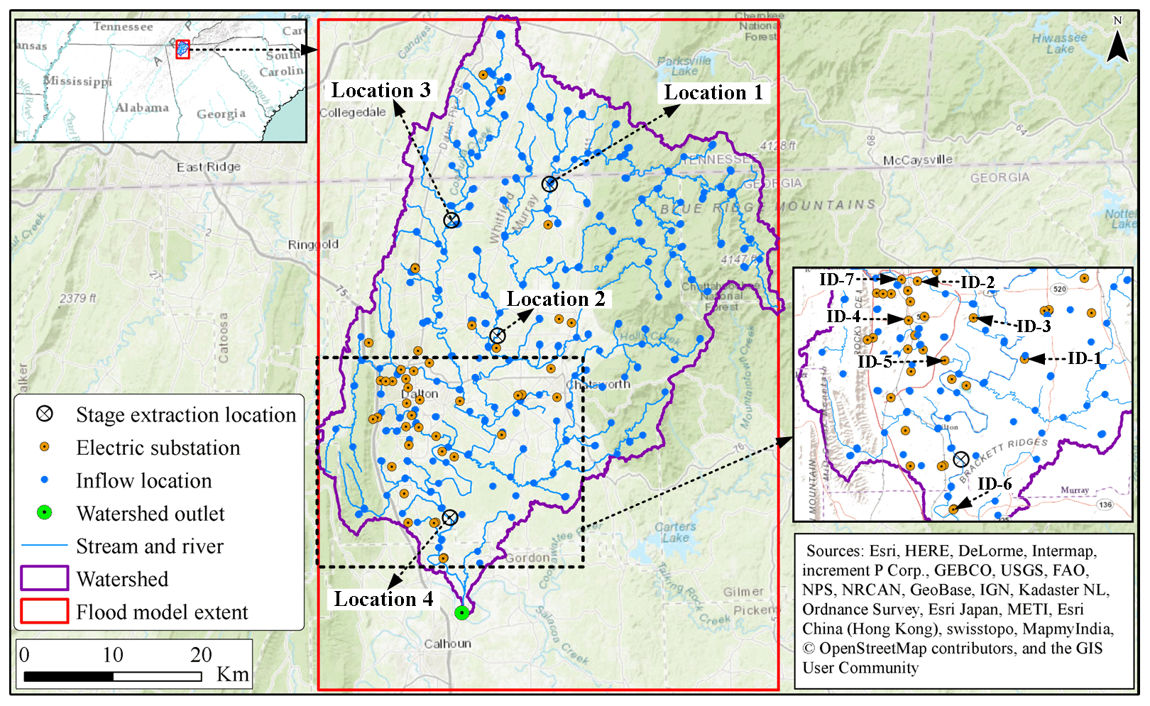
Figure 1Conasauga River watershed study area location, model extent, electric substations, and inflow locations. Background layer source: © OpenStreetMap contributors 2021. Distributed under a Creative Commons BY-SA License.
2.2 Streamflow projections
The ensemble streamflow projections were generated by a hierarchical modeling framework, which started with regional climate downscaling followed by hydrologic modeling (Gangrade et al., 2020). The climate projections were generated by dynamically downscaling 11 GCMs from the Coupled Model Intercomparison Project Phase-5 (CMIP5) data archive. Each GCM was used as lateral and lower boundary forcing in a regional climate model RegCM4 (Giorgi et al., 2012) at a horizontal grid spacing of 18 km over a domain that covered the continental US and parts of Canada and Mexico (Ashfaq et al., 2016) (Table 1). Each RegCM4 integration covered 40 years in the historic period (1966–2005; hereafter baseline) and another 40 years in the future period (2011–2050) under the Representative Concentration Pathway 8.5 (RCP8.5) emission scenario, with a combined 880 years of data across all RegCM4 simulations. To capture the multi-decadal climate variability, a minimum period of 30 years has been used in many studies (e.g., Alfieri et al., 2015a, b). Given the additional data available from Gangrade et al.(2020), we have adopted a longer 40-year period that may further enlarge the sample space to better support the statistical analyses in this study.
Table 1Summary of the 11 dynamically downscaled climate models (adopted from Ashfaq et al., 2016).

The RegCM4 simulated daily precipitation and temperature were further statistically bias-corrected to a spatial resolution of 4 km following a quantile mapping technique, described in Ashfaq et al. (2010, 2013). The 4 km Parameter-elevation Regressions on Independent Slopes Model (PRISM; Daly et al., 2008) data were used as the historic observations to support bias correction. In the baseline period, the simulated quantiles of precipitation and temperature were corrected by mapping them onto the observed quantiles. In the future period, the monthly quantile shifts were calculated based on the simulated baseline and future quantiles which were subsequently added to the bias-corrected baseline quantiles to generate bias-corrected monthly future data. Finally, the original daily values were rescaled to meet the corrected monthly precipitation and temperature. This approach substantially improves the biases in the modeled daily precipitation and temperature while preserving the simulated climate change signal. Further details of the bias correction are provided in Ashfaq et al. (2010, 2013) while the information regarding the RegCM4 configuration, evaluation, and future climate projections is detailed in Ashfaq et al. (2016).
The hydrologic simulations were then conducted using the Distributed Hydrology Soil Vegetation Model (DHSVM; Wigmosta et al., 1994), which is a process-based high-resolution hydrologic model that can capture heterogeneous watershed processes and meteorology at a fine resolution. DHSVM uses spatially distributed parameters, including topography, soil types, soil depths, and vegetation types. The input meteorological data include precipitation, incoming shortwave and longwave radiation, relative humidity, air temperature, and wind speed (Wigmosta et al., 1994, 2002; Storck et al., 1998). The DHSVM performance and applicability have been reported in various earlier climate- and flood-related studies (Elsner et al., 2010; Hou et al., 2019; Gangrade et al., 2018, 2019, 2020). A calibrated DHSVM implementation from Gangrade et al. (2018) at 90 m grid spacing was used to produce 3-hourly streamflow projections using the RegCM4 meteorological forcings described in the previous section (Table 1). In addition, a control simulation driven by 1981–2012 Daymet meteorologic forcings (Thornton et al., 1997) was conducted for model evaluation and validation. The hydrologic simulations used in this study are a part of a larger hydroclimate assessment effort for the ACT River basin, as detailed in Gangrade et al. (2020). Since there is no major reservoir in the CRW, the additional reservoir operation module (Zhao et al., 2016) was not needed in this study.
Note that while the ensemble streamflow projections based on dynamical downscaling and high-resolution hydrologic modeling from Gangrade et al. (2020) are suitable to explore extreme hydrologic events in this study, they do not represent the full range of possible future scenarios. Additional factors such as other GCMs, RCP scenarios, downscaling approaches, and hydrologic models and parameterization may also affect future streamflow projections. In other words, although these ensemble streamflow projections can tell us how likely the future streamflow magnitude may change from the baseline level, they are not the absolute prediction into the future. In practice, these modeling choices will likely be study-specific based on the agreement among key stakeholders. It is also noted that the new Coupled Model Intercomparison Project Phase-6 (CMIP6) data have also become available to update the ensemble streamflow projections but is not pursued in this study.
2.3 Inundation modeling
The ensemble inundation modeling was performed using TRITON, which is a computationally enhanced version of Flood2D-GPU (Kalyanapu et al., 2011). TRITON allows parallel computing using multiple graphics processing units (GPUs) through a hybrid Message Passing Interface (MPI) and Compute Unified Device Architecture (CUDA) (Morales-Hernández et al., 2021). TRITON solves the nonlinear hyperbolic shallow water equations using an explicit upwind finite-volume scheme, based on Roe's linearization. The shallow water equations are a simplified version of the Navier–Stokes equations in which the horizontal momentum and continuity equations are integrated in the vertical direction (see Morales-Hernández et al., 2021, for further model details). An evaluation of TRITON performance for the CRW is presented and discussed in Sect. 3.3.
TRITON's input data include digital elevation model (DEM), surface roughness, initial depths, flow hydrographs, and inflow source locations (Kalyanapu et al., 2011; Marshall et al., 2018; Morales-Hernández et al., 2020, 2021). In this study, the hydraulic and geometric parameters from the flood model evaluation section (Sect. 3.3) were used in the flood simulation. The topography was represented using the one-third arc-second (∼ 10 m) spatial resolution DEM (Archuleta et al., 2017) from the US Geological Survey (USGS). To improve the quality of the base DEM, as discussed in the flood model evaluation section, the main channel elevation was reduced by 0.15 m. Elevated roads and bridges that obstruct the flow of water were also removed. For surface roughness, we used a single channel Manning's n value of 0.05 and a single floodplain Manning's n value of 0.35. The selection of channel and floodplain Manning's n value was based on the Whitfield County Flood Insurance Study (FIS, 2007), which reported a range of Manning's n values estimated from field observations and engineering judgment for about 15 streams inside the CRW (Sect. 3.2). Furthermore, a water depth value of 0.35 m was defined for the main river channel as an initial boundary condition. The zero velocity gradients were used as the downstream boundary condition. Further discussion of model parameter sensitivity and model evaluation are provided in Sect. 3.2 and 3.3.
The simulated DHSVM streamflow was used to prepare inflow hydrographs for ensemble inundation modeling. To provide a large sample size for frequency analysis, we selected all annual maximum peak streamflow events (the maximum corresponded to the outlet of CRW Fig. 1) from the 1981–2012 control simulation (32 years), the 1966–2005 baseline simulation (440 years; 40 years × 11 models), and the 2011–2050 future simulation (440 years; 40 years × 11 models), with a total of 912 events. For each annual maximum event, the 3 h time step and 10 d hydrographs (which capture the peak CRW outlet discharge) across all DHSVM river segments were summarized. Following a procedure similar to Gangrade et al. (2019), these streamflow hydrographs were converted to TRITON inputs at 300 inflow locations selected along the NHD+ river network in the CRW (Fig. 1). The TRITON model extent, shown in Fig. 1, has an approximate area of 3945 km2 and includes ∼ 44 million model grid cells (7976 rows × 5474 columns in a uniform structured mesh). The ensemble flood simulations resulted in gridded flood depth and velocity output at 30 min intervals. The simulations generated approximately 400 TB of data and utilized ∼ 2000 node hours on the Summit supercomputer, managed by the Oak Ridge Leadership Computing Facility at Oak Ridge National Laboratory.
2.4 Flood inundation frequency analysis
Given the nature of GCM experiments, each set of climate projections can be considered a physics-based realization of historic and future climate under specified emission scenarios. Therefore, an ensemble of multimodel simulations can effectively increase the data lengths and sample sizes that are keys to support frequency analysis, especially for low-AEP events. In this study, we conducted flood frequency analyses separately for the 1966–2005 baseline and 2011–2050 future periods so that the difference between the two periods represents the changes in flood risk due to climate change.
To prepare the flood frequency analysis, we first calculated the maximum flood depth at every grid in each simulation. A minimum threshold of 10 cm flood depth was used to judge whether a cell was wet or dry (Gangrade et al., 2019). Further, for a given grid cell, if the total number of non-zero flood depth values (i.e., of the 440 depth values) was fewer than 30, the grid cell was also considered dry. This threshold was selected based on the minimum sample size requirement for flood depth frequency analysis suggested by Li et al. (2018). Next, we calculated the maximum flooded area (hereafter used alternatively with “floodplain area”) for each simulation. A log-Pearson type III (LP3) distribution was then used for frequency analysis following the guidelines outlined in Bulletins 17B (USGS, 1982; Burkey, 2009) and 17C (England et al., 2019). Two types of LP3 fitting were performed. The first type of fitting is event-based that fitted LP3 on the maximum inundation area across all ensemble members. The second type of fitting is grid-based (more computationally intensive) that fitted LP3 on the maximum flood depth at each grid cell across all ensemble members. For both types of fittings, the frequency estimates at 4 %, 2 %, 1 %, and 0.5 % AEP (corresponding to 25-, 50-, 100-, and 200-year return levels) were derived for further analysis.
It is also noted that in addition to the annual maximum event approach used in this study, one may also use the peak-over-threshold (POT) approach which can select multiple streamflow events in a very wet year. While such an approach can lead to higher extreme streamflow and inundation estimates, the timing of POT samples is fully governed by the occurrences of wet years. In other words, if the trend of extreme streamflow is significant in the future period, the POT samples will likely occur more in the far future period. We hence select the annual maximum event approach that can sample maximum streamflow events more evenly in time, which can better capture the evolution of extreme events with time under the influence of climate change.
2.5 Vulnerability of electricity infrastructure
The vulnerability of electricity infrastructures to climate-change-induced flooding was evaluated using the ensemble flood inundation results. The 44 electric substations (Fig. 1) collected from the publicly available Homeland Infrastructure Foundation-Level Data (HIFLD, 2019) were considered to be the electrical components susceptible to flooding. To evaluate the vulnerability of these substations, we overlapped the maximum flood extent from each ensemble member with all substations to identify the substations that might be inundated under the baseline and future climate conditions. Further, as an additional flood hazard indicator, the duration of inundation was estimated at each of the affected substations using the ensemble flood simulation results.
The vulnerability analysis was performed for two different flood mitigation scenarios. In the first scenario, we assumed that no flood protection measures were provided at all substations. Hence, the substations that intersected with the flood footprint were considered to be failed. In the second scenario, it was assumed that flood protection measures were adopted for all substations following the FEMA P-1019 recommendation (FEMA, 2014). According to FEMA P-1019 (FEMA, 2014), for emergency power systems within critical facilities, the highest elevation among (1) the base flood elevation (BFE: 1 % FEMA AEP flood elevation) plus 3 ft (∼ 0.91 m), (2) the locally adopted design flood elevation, and (3) the 500-year flood elevation can be used to design flood protection measures. Since the three recommended elevations were not available at all substation locations, we focused only on the BFE plus ∼ 0.91 m option. In addition, since in the CRW the majority of existing flood insurance maps were classified as Zone A – meaning that the special flood hazard areas were determined by approximate methods without BFE values (FEMA, 2002) – we used the maximum flood depth values across all control simulation years as the BFE values in this second mitigation scenario.
During the vulnerability analysis, we also assumed that (1) the one-third arc-second spatial resolution DEM might reasonably represent the elevation of substations, (2) existing substations would remain functional and would not be relocated, and (3) no additional hardening measures (i.e., protections such as levees, berms, anchors, and housings) will be adopted in the future period. Also, the cascading failure of a substation due to grid interconnection was not considered in this study.
3.1 Streamflow projections
This section presents a comparison of the annual maximum peak streamflow (at the outlet of CRW) used in the control, baseline, and future simulations. The sample size included 32 events from the control (1981–2012) simulation, 440 events from the baseline (1966–2005) simulations, and another 440 events from the future (2011–2050) simulations. These samples are illustrated in box-and-whisker plots in Fig. 2, where the central mark indicates the median, while the bottom and top edges indicate the 25th and 75th percentiles, respectively. The whiskers extend to the furthest data points not considered outliers, which correspond to approximately ±2.7 standard deviations and 99.3 % coverage if the data are normally distributed. As is evident from Fig. 2, the distributions of annual maximum peak streamflow values in the control and baseline simulations are comparable. The upper and lower whiskers in the control simulation are 727.6 and 84.2 m3/s, which compare well to the 722.5 and 65.2 m3/s values in the baseline simulation. In addition, we also conducted a two-tailed two-sample t test (α= 0.05) to compare whether the means of control and baseline annual maximum streamflow are statistically different. The results yielded a p value of 0.09, which suggested that there is no significant difference between the means of both control and baseline simulations. A larger number of outliers are present in the baseline simulation, which is due to the larger sample size (440 versus 32).
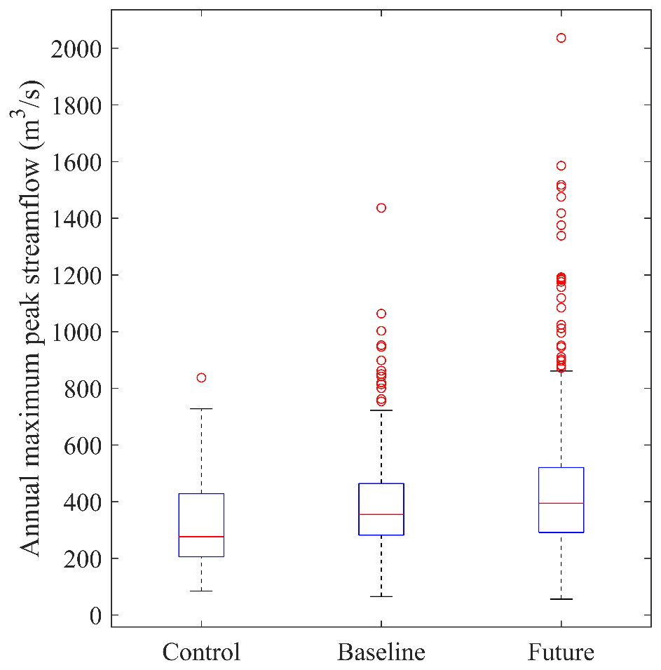
Figure 2A comparison of annual maximum peak streamflow at the outlet of the Conasauga River watershed. The sample size includes 32 events from the control (1981–2012), 440 from the baseline (1966–2005), and another 440 from the future (2011–2050) periods.
Under the future projection, an increase in the maximum peak streamflow is shown, where the upper whisker in the future projection is ∼ 21 % higher than the baseline. Moreover, the maximum of distribution in the future climate (2036.7 m3/s) is also much higher than that in the baseline climate (1436.7 m3/s), suggesting a higher future flood risk in the CRW. The increasing trend of streamflow extremes in the CRW is consistent with the overall findings in the ACT River basin (Gangrade et al., 2020).
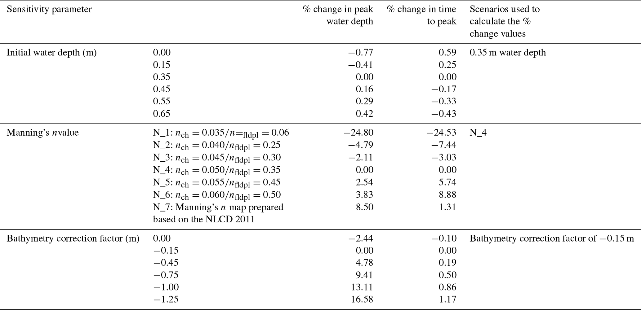
3.2 Sensitivity analysis for flood model
For a better understanding and selection of suitable TRITON parameters, a series of sensitivity analyses were conducted using different combinations of Manning's roughness, initial water depths, and river bathymetry correction factors (Table 2).
Table 2Summary of hydraulic and geometric parameters used in the sensitivity analysis.
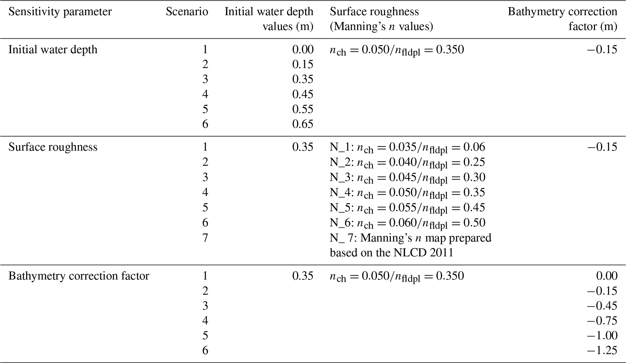
Note: nch represents the Manning's n value in the main channel and nfldpl represents the Manning's n value in the floodplain areas.
In calibrating a hydraulic model, it is a common practice to adjust the estimated Manning's n value, as it is the most uncertain and variable input hydraulic parameter (Brunner et al., 2016). In this study, we tested six different scenarios (Table 2) based on the Whitfield County Flood Insurance Study (FIS, 2007), which reported a range of Manning's n values estimated from field observations and engineering judgment for about 15 streams inside the CRW. It is noted that the depth variation in Manning's roughness is not considered in the current study. Readers are referred to studies such as Saksena et al. (2020) for additional information on the dynamic Manning's roughness for potential hydrology and hydraulics applications.
To establish an initial condition for TRITON, a sensitivity analysis was performed on selected initial water depth values (ranging from 0 to 0.65 m, Table 2) to understand their relative effects. To select ranges for the initial water depth, we summarized the observed water depth values that correspond to low flow values at five USGS gauge stations inside the CRW. The distribution of observed water depth values from the five gauges showed average values ranging from 0.25 to 0.65 m. Existing DEM products, even those with high spatial resolution (i.e., 10 m or finer), do not represent the elevation of river bathymetry accurately (Bhuyian et al., 2014). For the CRW, Bhuyian et al. (2019) found that the one-third arc-second spatial resolution base DEM over-predicted the inundation extent because of the bathymetric error, which reduced the channel conveyance. In this study, we tested various bathymetry correction factors (ranging from −1.25 to 0 m, Table 2) by reducing the DEM elevation along the main channel to understand the sensitivity of TRITON.
The sensitivity analysis was performed using the 13–22 February 1990 flood event that has the maximum discharge among all 32 control simulation events. To evaluate relative sensitivity of TRITON, we extracted simulated flood depths at four arbitrary selected locations (Fig. 1) and estimated the relative inundation area differences. The impacts of initial water depths were significant only at the beginning where low flow values dominated the hydrographs (Fig. 3a, d, g, and j). Larger initial water depth values generated higher flood inundation depths for all sample locations. Although the differences in flood inundation extents relative to the dry bed show an increasing trend, the relative differences are less than 1.4 % (Fig. 4a). Similarly, the differences in average peak water depths and time to peak relative to the 0.35 m initial water depth were less than 1.0 % (Table 3). Increase in the channel and floodplain Manning's n values resulted in higher flood depths for both sample locations (Fig. 3b, e, h, and k). The relative flood inundation area differences increase from about 23 % to 31 % (Fig. 4b) when the channel and floodplain Manning's n values are increased from 0.035 to 0.06 and from 0.06 to 0. 50, respectively. In terms of simulated maximum flood extent, the relative difference between scenario 3 (N_3) and scenario 7 (i.e., Manning's n map based on different land use types [N_7]) showed ∼ 16 % (22 km2) change in inundation area (Fig. 4b). Similarly, the last scenario (N_7) resulted in ∼ 9 % increase in the average peak water depth (Table 3), when compared to scenario 3 (N_3). Reduction in the elevation of river bathymetry (to improve the quality of the base DEM) results in a direct increase in maximum flood depth due to change in the river conveyance (Fig. 3c, f, i, and l; Table 3). It also results in a decrease in the maximum flood extent (Fig. 4c), as more water is allowed to transport through the main channel instead of the floodplain. Overall, the results showed that TRITON was more sensitive to the Manning's n values than the initial water depths and bathymetric correction factors.
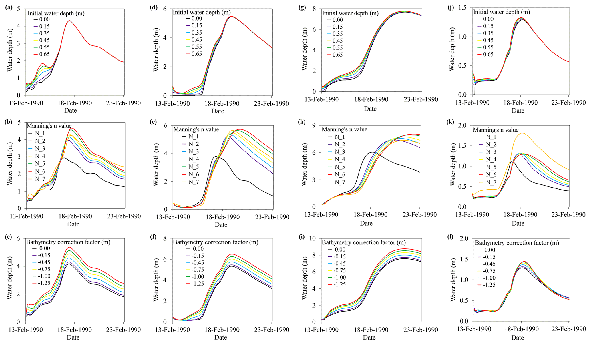
Figure 3Simulated flood inundation depths extracted at location 1 (a, b, c) and at location 2 (d, e, f). Note: locations 1 and 2 are shown in Fig. 1. A description of the Manning's n values (N_1 to N_6) can be found in Table 2.
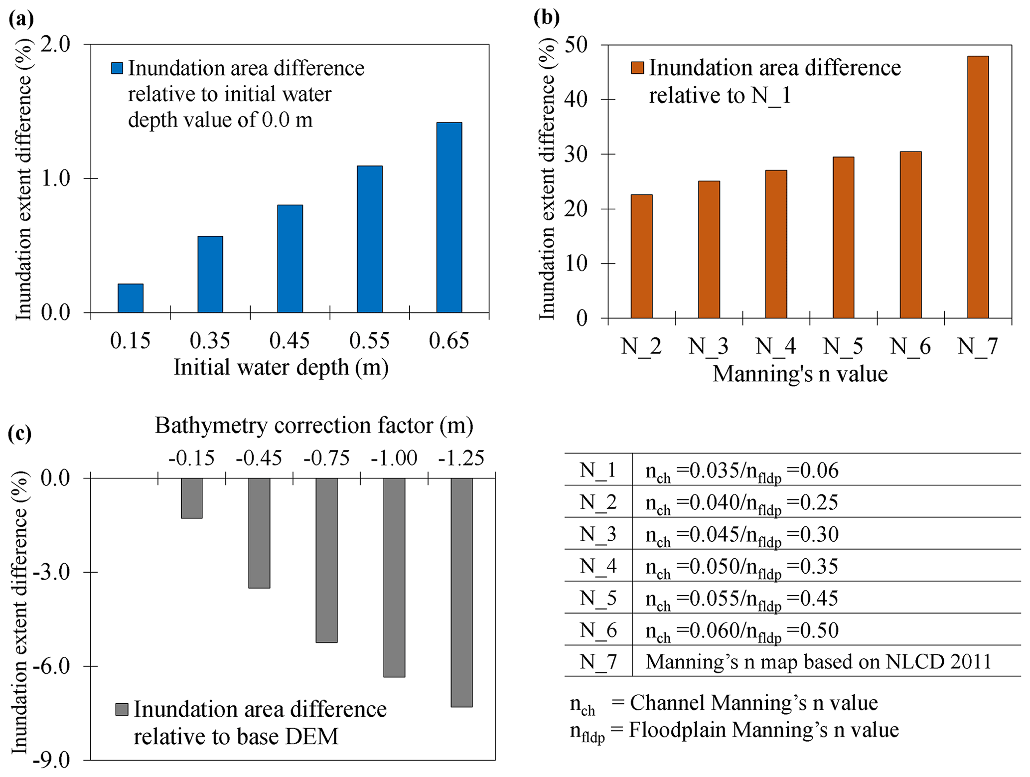
Figure 4Change in simulated maximum flood inundation extents for (a) initial water depth, (b) Manning's n value, and (c) bathymetry correction factor.
3.3 Flood model evaluation
Because of a lack of observed streamflow data in the CRW, the performance of TRITON was evaluated by comparing the simulated 1 % AEP flood map with the published 1 % AEP flood map from FEMA (FEMA, 2019). The purpose of this assessment is to understand whether TRITON can provide comparable results to the widely accepted FEMA flood estimates. While the FEMA AEP flood maps do not necessarily represent complete ground truth, such a comparison is the best option given the data challenge. A similar approach has been utilized by several previous studies in the evaluation of large-scale flood inundation (Alfieri et al., 2014; Wing et al., 2017; Zheng et al., 2018; Gangrade et al., 2019).
To derive the 1 % AEP flood map using TRITON, the ensemble-based approach used by Gangrade et al. (2019) was followed. The assessment started by preparing the streamflow hydrographs used to construct the 1 % AEP flood map. The 1981–2012 annual maximum peak events and their corresponding 10 d streamflow hydrographs were extracted from the control simulation. These streamflow hydrographs were then proportionally rescaled to match the 1 % AEP peak discharge estimated at the watershed outlet (Fig. 1), following the frequency analysis procedures outlined in Bulletin 17C (England et al., 2019). The streamflow hydrographs from control simulations were used for the peak discharge frequency analysis.
The results reported in the sensitivity analysis were also used to help identify suitable TRITON parameters. In addition to streamflow hydrographs, TRITON requires DEM, initial water depth, and Manning's n value. To minimize the effect of bathymetric error in the base DEM (Bhuyian et al., 2014, 2019), we reduced the elevation along the main channel by 0.15 m (i.e., a bathymetry correction factor). Although this simple approach is unlikely to adjust the channel bathymetry to its true values, it can improve the channel conveyance volume that is lost in the base DEM. To further improve the quality of the base DEM, we removed elevated roads and bridges that could obstruct the flow of water in some of the streams and rivers. An initial water depth of 0.35 m was also selected in this study. For the surface roughness, a couple of flood simulations were performed by adjusting the Manning's n values for the main channel and floodplain to achieve satisfactory agreement between the simulated and the reference FEMA flood map. We eventually selected a single channel Manning's n value of 0.05 and a single floodplain Manning's n value of 0.35.
Three evaluation metrics, including fit, omission, and commission (Kalyanapu et al., 2011) were used to quantify the differences between the modeled and reference flood map. The measure of fit determines the degree of relationship, while the omission and commission statistically compare the simulated and reference FEMA flood maps (Kalyanapu et al., 2011). The comparison between the simulated maximum inundation and the corresponding 1 % AEP FEMA flood map showed 80.65 % fit, 5.52 % commission, and 15.36 % omission (Fig. 5), demonstrating that the TRITON could reasonably estimate flood inundation extent and depths in the CRW. The computational efficiency of TRITON can further support ensemble inundation modeling to provide additional variability information that cannot be provided by the conventional deterministic flood map.
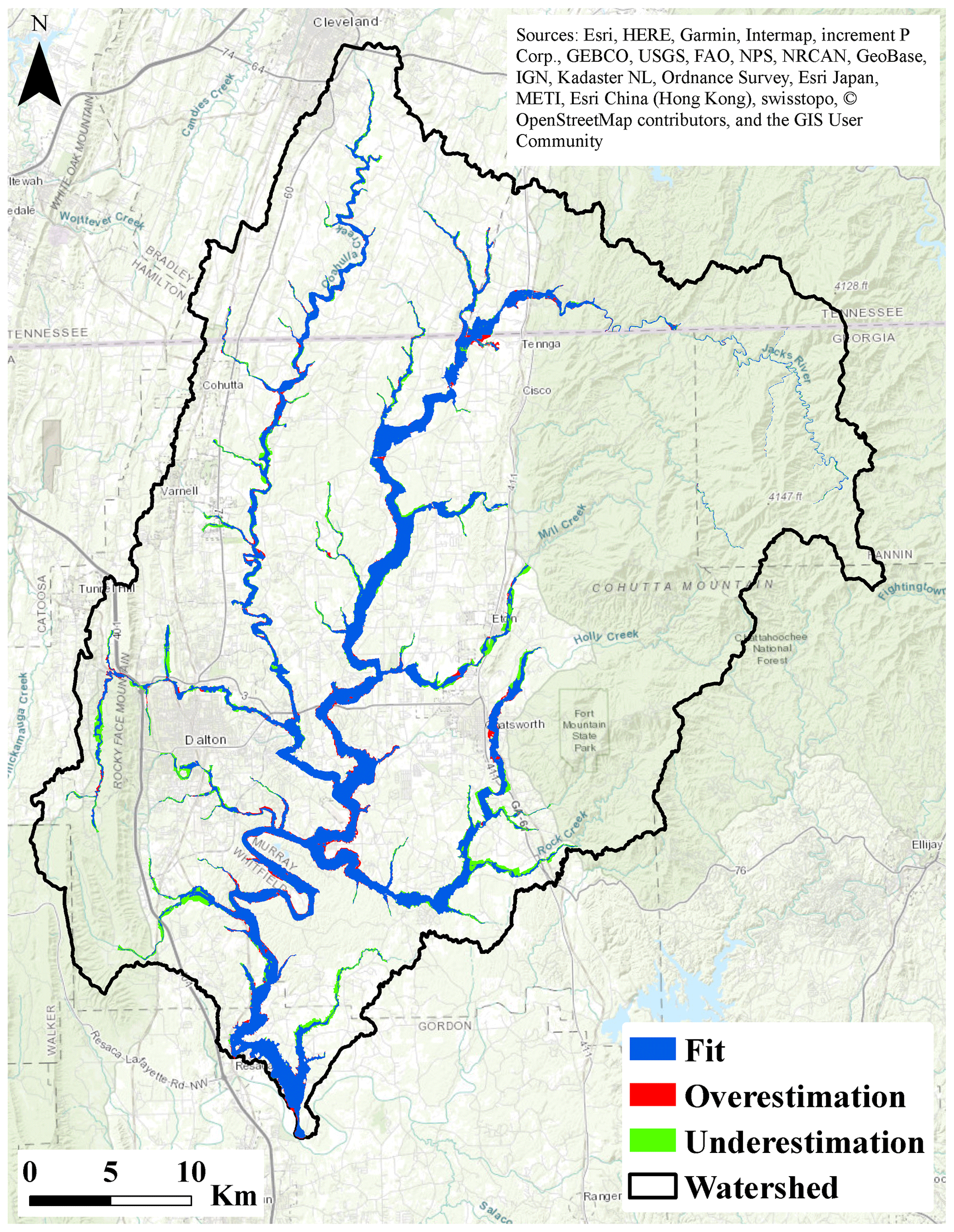
Figure 5Comparison of simulated maximum flood extent with the corresponding FEMA 1 % AEP flood map for the Conasauga River watershed. Background layer source: © OpenStreetMap contributors 2021. Distributed under a Creative Commons BY-SA License.
Although we have obtained satisfactory model performance for the purpose of our study, the flood model implementation has some limitations that may be enhanced in future studies. They include the following.
-
Spatially varying Manning's n values may be derived based on high-resolution land-use and land-cover (LULC) conditions to better represent the spatial heterogeneity in the modeling domain.
-
Apart from changes in future runoff and streamflow, projections of future LULC and its corresponding surface roughness can be considered to understand the broader impacts due to environment change.
-
In this study, we corrected DEM bias along the river channel cells by simplified bathymetry correction factors. More sophisticated bathymetric configuration (i.e., channel shape and sinuosity) can be considered to better represent channel conveyance.
-
The current TRITON model does not provide capability to route local runoff and external inflows through stormwater drainage systems. Coupling with additional stormwater drainage models can be a potential future direction.
-
Hydraulic and civil structures such as bridges, culverts, and weirs have not been included since TRITON does not provide for the modeling of such components. This can affect the accuracy of the flood depths, velocities, and flood extents around these structures.
3.4 Change in flood regime
In this section, the projected changes in flood regime were calculated using the flooded area from the baseline and future simulations for each ensemble member. Figure 6 illustrates the box-and-whisker plots for each of the 11 dynamically downscaled GCMs. Given the small sample size in each distribution (40 compared to 440 in Fig. 2), the whiskers extend the largest and smallest data points with no outlier detection. For 9 out of the 11 downscaled climate models, the mean of 40 flood inundation showed an increase in the floodplain area in the future period. In terms of the 75th percentile and maximum, 10 out of 11 models showed an increase in the floodplain area. The distributions of maximum future inundation of four models are found to be statistically different than their baseline distributions at a 5 % significance level. Note that the spread in the future period is generally larger than the spread in the baseline period, suggesting an increase in the hydrologic variability in the future period. Also, while the results from different models were generally consistent, some inter-model differences were noted, which highlight the need of a multi-model framework to capture the uncertainty in the future climate projections. The multi-model approach provides a range of possible flood inundation extents, which is critical for floodplain management decision making. The potential increase in the floodplain area also demonstrates the importance of incorporating climate change projections in the floodplain management regulations.
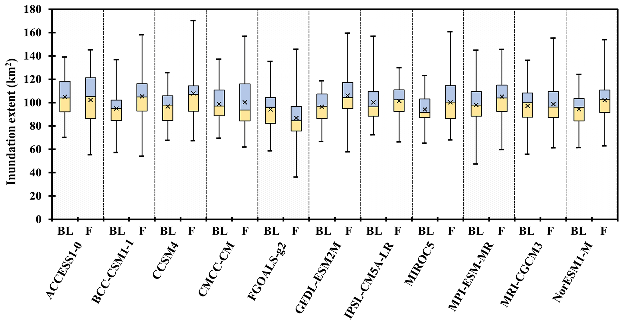
Figure 6A summary of simulated maximum flood inundation extents obtained from the baseline and future scenarios. The mean flooded area values are shown by × symbols. Note: the suffix “_BL” represents baseline scenarios and the suffix “_F” represents future scenarios.
3.5 Flood inundation frequency curve and map
Figure 7 shows the relationship between the 440 flooded area values (across 11 downscaled GCMs) and their corresponding peak streamflow at the watershed outlet, for both the baseline and future periods. Overall, both results (Fig. 7a and b) exhibit strong nonlinear relationships with high R2 values. The results suggest that peak streamflow is a significant variable controlling the total flooded area, but the variability of flooded area could not be explained by peak streamflow alone. For instance, in the baseline period, the peak streamflow values of 423.63 and 424.25 m3/s correspond to 106.85 and 94.89 km2 floodplain areas, respectively (Fig. 7a). Similarly, in the future period, the peak streamflow values of 433.27 and 434.21 m3/s correspond to 110.76 and 99.26 km2 floodplain areas (Fig. 7b).

Figure 7Relationship between floodplain areas and peak streamflow values at the watershed outlet for (a) baseline and (b) future scenarios. The blue lines indicate the logarithmic best fit.
Figure 8 shows the event-based flood inundation frequency curves and their corresponding 95 % confidence intervals in both the baseline and future periods, for which each frequency curve was derived using an ensemble of 440 years of data. The use of long-term data helped reduce the uncertainty and add more confidence in the evaluation of the lower AEP estimates. This type of assessment cannot be achieved using only historic streamflow observations, for which the limited records present a major challenge for lower AEP estimates. For most of the exceedance probabilities, the flooded areas projected an increase in the inundation areas in the future period when compared to the baseline period. The 1 % AEP flood shows an ∼ 16 km2 increase in the inundation area (137.75 km2 in the baseline period versus 153.43 km2 in the future period) (Fig. 8). Similar results can be observed in inundation frequency curves developed for other AEPs (not shown).
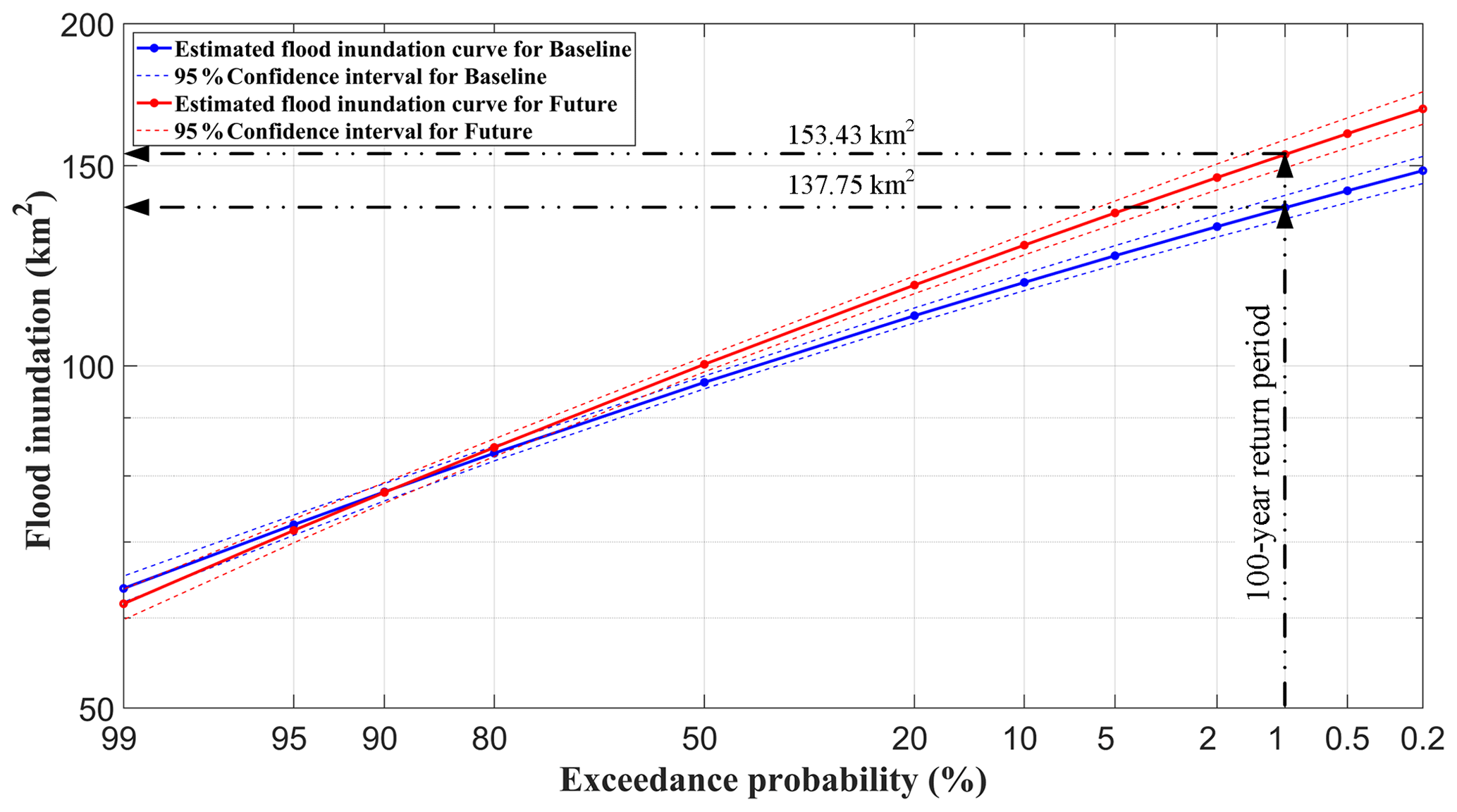
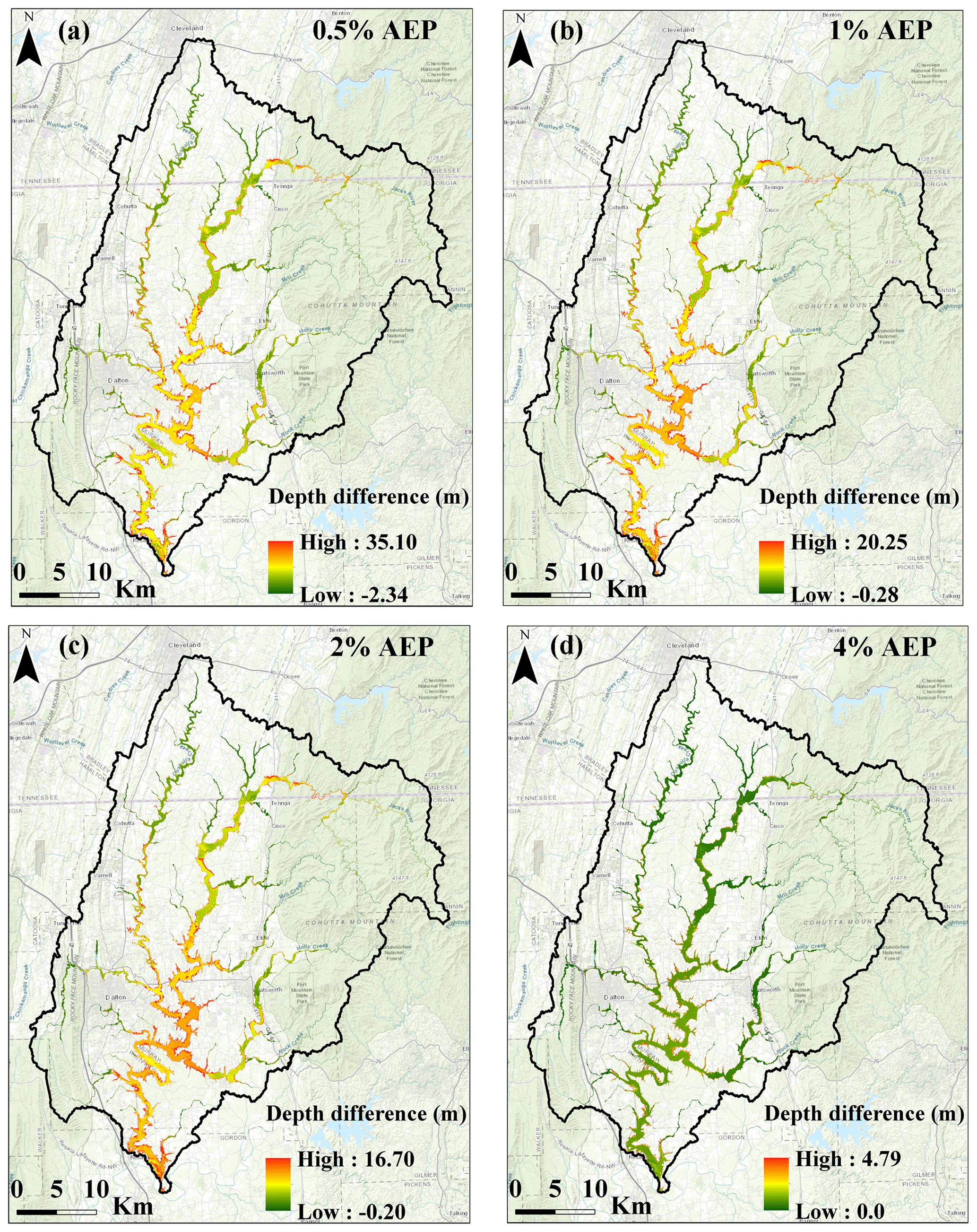
Figure 9Projected change (future minus baseline period) in flood depth frequency maps for (a) 0.5 %, (b) 1 %, (c) 2 %, and (d) 4 % AEPs. ArcGIS background layer sources: ESRI, HERE, Garmin, Intermap, GEBCO, USGS, Food and Agriculture Organization, National Park Service, Natural Resources Canada, GeoBase, IGN, Kadaster NL, Ordnance Survey, METI, Esri Japan, Esri China, the GIS User Community, and © OpenStreetMap contributors 2021. Distributed under a Creative Commons BY-SA License.
The grid-based flood depth frequency results at 0.5 %, 1 %, 2 %, and 4 % AEP levels are illustrated in Fig. 9. In each panel, the projected change (i.e., future minus baseline) at each grid is shown. The corresponding histogram across the entire study area is presented in Fig. 10. As mentioned in Sect. 2.4, the LP3 distribution was used for frequency analysis. In order to understand the suitability of LP3, we also conducted a comparative analysis to test an alternative log-normal (LN) distribution. By using the Anderson–Darling (Anderson and Darling, 1952) goodness-of-fit test (α=0.05) along with the Akaike information criterion (Akaike, 1974), we found no substantial difference between these two distributions (not shown), for the purpose of our application. It is noted, however, that our goal in this study is not to identify the most suitable choice of flood depth distribution. Therefore, other more suitable distributions may exist but that is beyond the scope of this study.
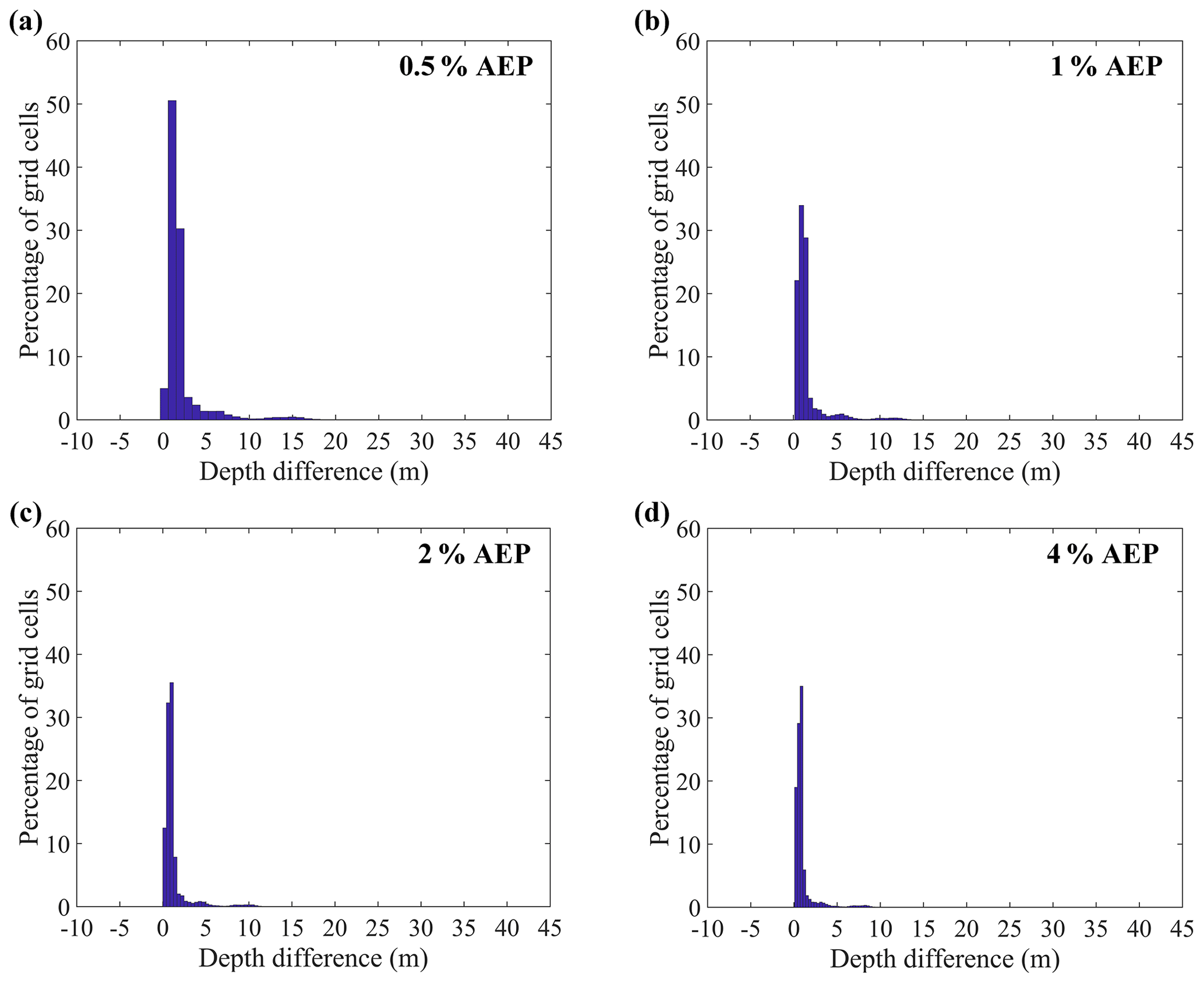
Figure 10Histograms for the future changes (2011–2050) in the flood depth relative to the baseline period (1966–2005) for (a) 0.5 %, (b) 1 %, (c) 2 %, and (d) 4 % AEP flood depth frequency maps.
Based on the comparisons in Fig. 10, it is estimated that the flood depth values at ∼ 80 % of grid cells would increase by 0.2 to 1.5 m due to projected changes in climate (Fig. 10). For 0.5 % and 1 % AEP flood depth frequency maps (Fig. 9a and b), the changes in flood depth were more pronounced in the lower part of the CRW, near the city of Dalton (where there are large population settlements), thereby increasing the likelihood of population exposure to flood risk in the future period. Furthermore, for the 1 % flood depth frequency map (Fig. 9b), the projected increase in flood depths and spatial extent has the potential to extend the flood damage far beyond the FEMA's current base floodplain area. Therefore, these results highlight the need for climate change consideration in the floodplain mapping. The approach presented in this study can provide an alternative floodplain delineation technique, as it can be applied to develop flood depth frequency maps that are reflective of the future climate.
3.6 Vulnerability of electricity infrastructure
Figure 11a shows the box-and-whisker plot for the distributions of maximum flood depth values extracted at the substation location across all the baseline and future simulations, assuming that no flood protection measures were adopted (mitigation scenario 1). Of the 44 substations, 5 substations could have been affected during the baseline period, while 7 substations are projected to be affected during the future period (Fig. 11a). Increases are indicated not only for the number of affected substations but also for flood inundation depth values in the projected future climate. Overall, the mean of the ensemble flood depth values shows an ∼ 0.6 m increase in the future period (Fig. 11a). Such an increase in the flood depth magnitude has the potential to exacerbate flood-related damage to electrical components, which can inflate the cost of hardening measures such as elevating substations and constructing flood-protective barriers. As expected, when the substations were flood-proofed up to BFE plus ∼ 0.91 m (mitigation scenario 2), the number of affected substations is reduced to three and four during the baseline and future periods, respectively (Fig. 11b). The locations of substations that were impacted in the baseline period, in both mitigation scenarios, are consistent with the Whitfield County Emergency Management Agency report map (EMA, 2016) that shows the locations of critical facilities vulnerable to the historical flooding.
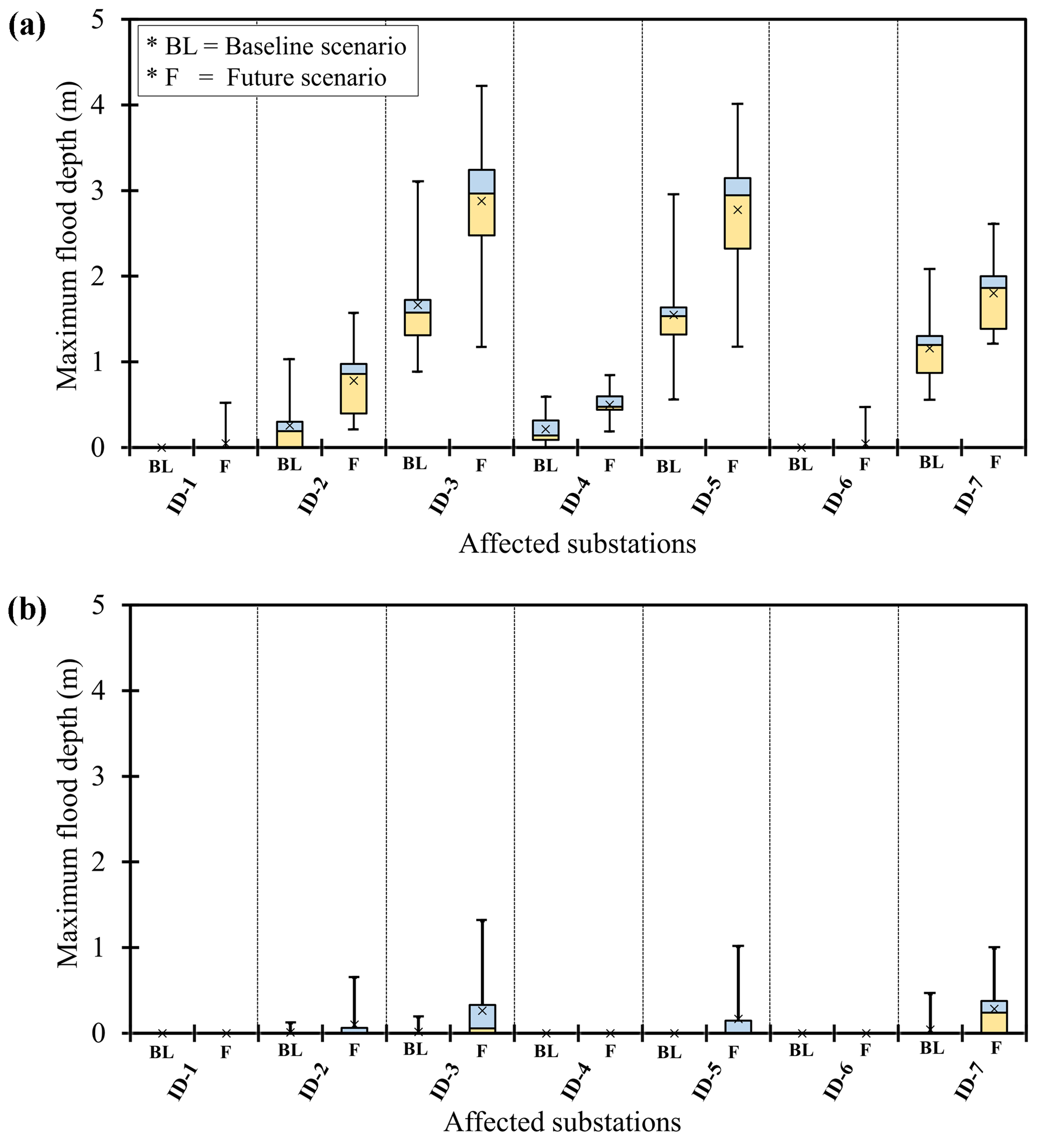
Figure 11A summary of maximum flood depths for substations that were affected in the baseline and/or future periods (a) without flood protection measures and (b) with flood protection measures. Note: affected substations with their corresponding IDs are shown in Fig. 1. There are no negative values in the vertical axis, as the minimum flood depth value is zero.

Figure 12A summary of maximum inundation durations for substations that were affected in the baseline and/or future periods (a) without flood protection measures and (b) with flood protection measures. Note: affected substations with their corresponding IDs are shown in Fig. 1. There are no negative values on the vertical axis, as the minimum inundation duration is zero.
The maximum inundation durations at the affected substations are summarized in Fig. 12a (mitigation scenario 1) and b (mitigation scenario 2). For both mitigation scenarios and all affected substations, ensemble mean inundation durations exhibited an increase under future climate conditions. This increase in inundation duration would probably render substations out of service for longer periods of time by making it difficult to repair damaged substation equipment and restore grid services to customers. The potential hazards and consequences may also extend to critical facilities that are supplied by the affected substations. Similar to results presented in the previous sections, these results demonstrate the need for improving existing flood mitigation measures by incorporating the trends and uncertainties that originate from climate change. The vulnerability analysis approach presented in this study will better equip floodplain managers to identify the most vulnerable substations and to recommend suitable adaptation measures, while allocating resources efficiently.
This paper applies an integrated modeling framework to evaluate climate change impacts on flood regime, floodplain protection standards, and electricity infrastructures across the Conasauga River watershed in the southeastern United States. Building on the ensemble concept used by Gangrade et al. (2019) for PMF-scale inundation modeling (AEP < 10−4 %), we focused on more frequent extreme streamflow events (i.e., AEP around 1 %–0.2 %) based on 11 downscaled CMIP5 GCMs in this study. Our evaluation is based on a climate–hydrologic–hydraulic modeling framework, which makes use of an 11-member ensemble of downscaled climate simulations. A total of 9 out of 11 ensemble members project an increase in the flood inundation area in the future period. Similarly, at the 1 % AEP level, the flood inundation frequency curves indicate ∼ 16 km2 increase in floodplain area under the future climate. The comparison between the flood depth frequency maps from the baseline and future simulations indicated that, on average, ∼ 80 % of grid cells exhibit a 0.2 to 1.5 m increase in the flood depth values. Without the flood protection measures, of the 44 electric substations inside the watershed, 5 and 7 substations could be affected during the baseline and future periods, respectively. Even after flood-proofing, three and four substations could still be affected in the baseline and future periods. The increases in flood depth magnitude and inundation duration at the affected substations in the future period will most likely damage more electrical components, inflate the cost of hardening measures, and render substations out of service for a longer period of time.
Although future climate conditions are uncertain, our results demonstrate the needs for (1) consideration of climate change in the floodplain management regulations, (2) improvements in the conventional deterministic flood delineation approach through the inclusion of probabilistic or ensemble-based methods, and (3) improvements in the existing flood protection measures for critical electricity infrastructures through enhanced hydro-meteorologic modeling capacities. In particular, rapidly advanced high-performance computing capabilities have enabled the incorporation of computationally intensive 2D hydraulics modeling in the ensemble-based hydroclimate impact assessment. While the computational cost demonstrated in this study may still seem steep, in the current speed of technology advancement, we will soon be able to implement such a computationally intensive assessment for wide applications. The approach presented in this study can be used by floodplain managers to develop flood depth frequency maps and to identify the most vulnerable electric substations.
The data that support the findings of this study are openly available in the figshare repository at the following URLs: https://doi.org/10.6084/m9.figshare.12330929.v2 (Kalyanapu and Dullo, 2020a) and https://doi.org/10.6084/m9.figshare.12330917.v1 (Kalyanapu and Dullo, 2020b).
TTD, AJK, SCK, SG, and MMH developed the concept for the paper and designed the methodology. TTD performed all the simulations required for the study with feedback from all the co-authors. MBS, SG, and MMH focused on programming, software development, and testing of existing code components. MA and MMH provided access to supercomputing machine hours on ORNL's SUMMIT and RHEA computers. The manuscript was edited by TTD with inputs from the co-authors.
The authors declare that they have no conflict of interest.
This study was supported by the US Air Force Numerical Weather Modeling Program. Tigstu T. Dullo, M. Bulbul Sharif, Alfred J. Kalyanapu, and Sudershan Gangrade also acknowledge support by the Center of Management, Utilization, and Protection of Water Resources at Tennessee Technological University. Some portion of the project was funded by UT-Battelle subcontract no. 4000164401. The research used resources of the Oak Ridge Leadership Computing Facility at Oak Ridge National Laboratory. The input data sets are cited throughout the paper, as appropriate.
This research has been supported by the US Air Force Numerical Weather Modeling Program.
This paper was edited by David J. Peres and reviewed by two anonymous referees.
AECOM: The Impact of Climate Change and Population Growth on the National Flood Insurance Program through 2100, available at: https://www.aecom.com/content/wp-content/uploads/2016/06/Climate_Change_Report_AECOM_2013-06-11.pdf (last access: 12 October 2019), 2013.
Akaike, H.: A new look at the statistical model identification, IEEE Transactions on Automatic Control, 19, 716–723, https://doi.org/10.1109/TAC.1974.1100705, 1974.
Alfieri, L., Salamon, P., Bianchi, A., Neal, J., Bates, P., and Feyen, L.: Advances in Pan-European Flood Hazard Mapping, Hydrol. Process., 28, 4067–4077, https://doi.org/10.1002/hyp.9947, 2014.
Alfieri, L., Burek, P., Feyen, L., and Forzieri, G.: Global warming increases the frequency of river floods in Europe, Hydrol. Earth Syst. Sci., 19, 2247–2260, https://doi.org/10.5194/hess-19-2247-2015, 2015a.
Alfieri, L., Feyen, L., Dottori, F., and Bianchi, A.: Ensemble Flood Risk Assessment in Europe Under High End Climate Scenarios, Global Environ. Change, 35, 199–212, https://doi.org/10.1016/j.gloenvcha.2015.09.004, 2015b.
Alfieri, L., Bisselink, B., Dottori, F., Naumann, G., de Roo, A., Salamon, P., Wyser, K., and Feyen, L.: Global Projections of River Flood Risk in a Warmer World, Earth's Future, 5, 171–182, https://doi.org/10.1002/2016EF000485, 2017.
Alfieri, L., Dottori, F., Betts, R., Salamon, P., and Feyen, L.: Multi-Model Projections of River Flood Risk in Europe under Global Warming, Climate, 6, https://doi.org/10.3390/cli6010006, 2018.
Allen-Dumas, M. R., Binita, K. C., and Cunliff, C. I.: Extreme Weather and Climate Vulnerabilities of the Electric Grid: A Summary of Environmental Sensitivity Quantification Methods, ORNL/TM-2019/1252, Oak Ridge National Laboratory, available at: https://www.energy.gov/sites/prod/files/2019/09/f67/Oak Ridge National Laboratory EIS Response.pdf, last access: 17 December 2019.
Anderson, T. W. and Darling, D. A. Asymptotic theory of certain “goodness-of-fit” criteria based on stochastic processes, Ann. Math. Stat., 23, 193–212, https://www.jstor.org/stable/2236446 (last access: 26 May 2021), 1952.
Archuleta, C.-A. M., Constance, E. W., Arundel, S. T., Lowe, A. J., Mantey, K. S., and Phillips, L. A.: The National Map Seamless Digital Elevation Model Specifications, US Geological Survey Techniques and Methods 11-B9, https://doi.org/10.3133/tm11B9, 2017.
Arnell, N. W. and Gosling, S. N.: The Impacts of Climate Change on River Flood Risk at the Global Scale, Clim. Change, 134, 387–401, doi.10.1007/s10584-014-1084-5, 2014.
Ashfaq, M., Bowling, L. C., Cherkauer, K., Pal, J. S., and Diffenbaugh, N. S.: Influence of Climate Model Biases and Daily-scale Temperature and Precipitation Events on Hydrological Impacts Assessment: A Case Study of the United States, J. Geophys. Res., 115, D14116, https://doi.org/10.1029/2009JD012965, 2010.
Ashfaq, M., Ghosh, S., Kao, S.-C., Bowling, L. C., Mote, P., Touma, D., Rauscher, S. A., and Diffenbaugh, N. S.: Near-term Acceleration of Hydroclimatic Change in the Western U.S., J. Geophys. Res., 118, 10676–10693, https://doi.org/10.1002/jgrd.50816, 2013.
Ashfaq, M., Rastogi, D., Mei, R., Kao, S.-C., Gangrade, S., Naz, B. S., and Touma, D.: High-resolution Ensemble Projections of Near-term Regional Climate over the Continental United States. J. Geophys. Res., 121, 9943–9963, https://doi.org/10.1002/2016JD025285, 2016.
Baechler, M. C., Gilbride, T. L., Cole, P. C., Hefty, M. G., and Ruiz, K.: Building America Best Practices Series, Volume 7.3, High-Performance Home Technologies: Guide to Determining Climate Regions by County, Pacific Northwest National Laboratory, US Department of Energy under Contract DE-AC05-76RLO 1830, PNNL-17211 Rev. 3, available at: https://www.energy.gov/sites/prod/files/2015/10/f27/ba_climate_region_guide_7.3.pdf (last access: 27 September 2020), 2015.
Bedient, P. B., Huber, W. C., and Vieux, B. E.: Hydrology and Floodplain Analysis, Prentice Hall, Upper Saddle River, New Jersey, 2013.
Bhuyian, Md. N. M., Kalyanapu, A. J., and Nardi, F.: Approach to Digital Elevation Model Correction by Improving Channel Conveyance, J. Hydrol. Eng., 20, 04014063, https://doi.org/10.1061/(ASCE)HE.1943-5584.0001020, 2014.
Bhuyian, Md. N. M., Dullo, T. T., Kalyanapu, A. J., Gangrade, S., and Kao, S.-C.: Application of Geomorphic Correlations for River Bathymetry Correction in Two-dimensional Hydrodynamic Modeling for Long-term Flood Risk Evaluation, World Environmental and Water Resources Congress, Pittsburgh, Pennsylvania, USA, 19–23 May 2019, 2019.
Birhanu, D., Kim, H., Jang, C., and Park, S.: Flood Risk and Vulnerability of Addis Ababa City Due to Climate Change and Urbanization, Procedia Engineer, 154, 696–702, https://doi.org/10.1016/j.proeng.2016.07.571, 2016.
Blessing, R., Sebastian, A., and Brody, S. D.: Flood Risk Delineation in the United States: How Much Loss Are We Capturing?, Nat. Hazards Rev., 18, 04017002, https://doi.org/10.1061/(ASCE)NH.1527-6996.0000242, 2017.
Bollinger, L. A. and Dijkema, G. P. J.: Evaluating Infrastructure Resilience to Extreme Weather – the Case of the Dutch Electricity Transmission Network, EJTIR, 16, 214–239, https://doi.org/10.18757/ejtir.2016.16.1.3122, 2016.
Bragatto, T., Cresta, M., Cortesi, F., Gatta, F. M., Geri, A., Maccioni, M., and Paulucci, M.: Assessment and Possible Solution to Increase Resilience: Flooding Threats in Terni Distribution Grid, Energies, 12, 744, https://doi.org/10.3390/en12040744, 2019.
Brunner, G. W., Warner, J. C., Wolfe, B. C., Piper, S. S., and Marston, L.: Hydrologic Engineering Center – River Analysis System (HEC-RAS) Applications Guide 2016, Version 5.0, US Army Corps of Engineers, CA, available at: https://www.hec.usace.army.mil/software/hec-ras/documentation/HEC-RAS 5.0 Applications Guide.pdf (last access: 27 December 2019), 2016.
Burkey, J.: Log-Pearson Flood Flow Frequency using USGS 17B, available at: https://www.mathworks.com/matlabcentral/fileexchange/22628-log-pearson-flood-flow-frequency-using-usgs-17b (last access: 23 December 2019), 2009.
Chandramowli, S. N. and Felder, F. A.: Impact of Climate Change on Electricity Systems and Markets – A Review of Models and Forecasts, Sustain. Energy Technol. Assess., 5, 62–74, https://doi.org/10.1016/j.seta.2013.11.003, 2014.
Ciscar, J. C. and Dowling, P.: Integrated Assessment of Climate Impacts and Adaptation in the Energy Sector, Energ. Econ., 46, 531–538, https://doi.org/10.1016/j.eneco.2014.07.003, 2014.
Cronin, J., Anandarajah, G., and Dessens, O.: Climate Change Impacts on the Energy System: A Review of Trends and Gaps, Clim. Change, 151, 79–93, https://doi.org/10.1007/s10584-018-2265-4, 2018.
Daly, C., Halbleib, M., Smith, J. I., Gibson, W. P., Doggett, M. K., Taylor, G. H., Curtis, J., and Pasteris, P. P.: Physiographically Sensitive Mapping of Climatological Temperature and Precipitation Across the Conterminous United States, Int. J. Climatol., 28, 2031–2064, https://doi.org/10.1002/joc.1688, 2008.
Elliott, K. J. and Vose, J. M.: Initial Effects of Prescribed Fire on Quality of Soil Solution and Streamwater in the Southern Appalachian Mountains, South. J. Appl. For., 29, 5–15, https://doi.org/10.1093/sjaf/29.1.5, 2005.
Elsner, M. M., Cuo, L., Voisin, N., Deems, J. S., Hamlet, A. F., Vano, J. A., Mickelson, K. E. B., Lee, S.-Y., and Lettenmaier, D. P.: Implications of 21st Century Climate Change for the Hydrology of Washington State, Climatic Change, 102, 225–260, https://doi.org/10.1007/s10584-010-9855-0, 2010.
England Jr., J. F., Cohn, T. A., Faber, B. A., Stedinger, J. R., Thomas Jr., W. O., Veilleux, A. G., Kiang, J. E., and Mason Jr., R. R.: Guidelines for Determining Flood Flow Frequency–Bulletin 17C, Techniques and Methods 4-B5, US Geological Survey, https://doi.org/10.3133/tm4B5, 2019.
Farber-DeAnda, M., Cleaver, M., Lewandowski, C., and Young, K.: Hardening and Resiliency: US Energy Industry Response to Recent Hurricanes Seasons, Office of Electricity Delivery and Energy Reliability, US Department of Energy, available at: https://www.oe.netl.doe.gov/docs/HR-Report-final-081710.pdf (last access: 17 December 2019), 2010.
FEMA (Federal Emergency Management Agency): Emergency Power Systems for Critical Facilities: A Best Practices Approach to Improving Reliability, FEMA P-1019, Applied Technology Council, Redwood City, CA, available at: https://www.fema.gov/media-library/assets/documents/101996 (last access: 17 December 2019), 2014.
FEMA (Federal Emergency Management Agency): FEMA Flood Map Service Center, available at: https://msc.fema.gov/portal/availabilitySearch?#searchresultsanchor, last access: 28 December 2019.
FIS (Flood Insurance Study): Flood Insurance Study: Whitfield County, Georgia and Incorporated Areas, Flood Insurance Study Number: 13313CV000A, Federal Emergency Management Agency, available at: https://georgiadfirm.com/pdf/panels/13313CV000A.pdf (last access: 25 December 2019), 2007.
FIS (Flood Insurance Study): Flood Insurance Study: Murray County, Georgia and Incorporated Areas, Flood Insurance Study Number: 13213CV000A, Federal Emergency Management Agency, available at: https://georgiadfirm.com/pdf/panels/13213CV000A.pdf (last access: 27 December 2019), 2010.
Forzieri, G., Bianchi, A., e Silva, F. B., Herrera, M. A. M., Leblois, A., Lavalle, C., Aerts, J. C. J. H., and Feyen, L.: Escalating Impacts of Climate Extremes on Critical Infrastructures in Europe, Global Environ. Chang., 48, 97–107, https://doi.org/10.1016/j.gloenvcha.2017.11.007, 2018.
Fu, G., Wilkinson, S., Dawson, R. J., Fowler, H. J., Kilsby, C., Panteli, M., and Mancarella, P.: Integrated Approach to Assess the Resilience of Future Electricity Infrastructure Networks to Climate Hazards, IEEE Syst. J., 12, 3169–3180, https://doi.org/10.1109/JSYST.2017.2700791, 2017.
Galloway, G. E., Baecher, G. B., Plasencia, D., Coulton, K. G., Louthain, J., Bagha, M., and Levy, A. R.: Assessing the Adequacy of the National Flood Insurance Program's 1 Percent Flood Standard, Water Policy Collaborative, University of Maryland, available at: https://www.fema.gov/media-library/assets/documents/9594 (last access: 17 December 2019), 2006.
Gangrade, S., Kao, S.-C., Naz, B. S., Rastogi, D., Ashfaq, M., Singh, N., and Preston, B. L.: Sensitivity of Probable Maximum Flood in a Changing Environment, Water Resour. Res., 54, 3913–3936, https://doi.org/10.1029/2017WR021987, 2018.
Gangrade, S., Kao, S.-C., Dullo, T. T., Kalyanapu, A. J., and Preston, B. L.: Ensemble-based Flood Vulnerability Assessment for Probable Maximum Flood in a Changing Environment, J. Hydrol., 576, 342–355, https://doi.org/10.1016/j.jhydrol.2019.06.027, 2019.
Gangrade, S., Kao, S.-C., and McManamay, R. A.: Multi-model Hydroclimate Projections for the Alabama-Coosa-Tallapoosa River Basin in the Southeastern United States, Sci. Rep.-UK, 10, 2870, https://doi.org/10.1038/s41598-020-59806-6, 2020.
Gilstrap, M., Amin, S., and DeCorla-Souza, K.: United States Electricity Industry Primer, DOE/OE-0017, Office of Electricity Delivery and Energy Reliability, US Department of Energy, Washington DC, available at: https://www.energy.gov/sites/prod/files/2015/12/f28/united-states-electricity-industry-primer.pdf (last access: 17 December 2019), 2015.
Giorgi, F., Coppola, E., Solmon, F., Mariotti, L., Sylla, M. B., Bi, X., Elguindi, N., Diro, G. T., Nair, V., Giuliani, G., Turuncoglu, U. U., Cozzini, S., Güttler, I., O'Brien, T. A., Tawfik, A. B., Shalaby, A., Zakey, A. S., Steiner, A. L., Stordal, F., Sloan, L. C., and Brankovic, C.: RegCM4: model description and preliminary tests over multiple CORDEX domains, Climate Res., 52, 7–29, https://doi.org/10.3354/cr01018, 2012.
HCFCD (Harris County Flood Control District): Hurricane Harvey – Storm and Flood Information, available at: https://www.hcfcd.org/Portals/62/Harvey/immediate-flood-report-final-hurricane-harvey-2017.pdf (last access: 16 December 2019), 2018.
HIFLD (Homeland Infrastructure Foundation-Level Data): Homeland Infrastructure Foundation-Level Data, Electric Substations, US Department of Homeland Security, available at: https://hifld-geoplatform.opendata.arcgis.com/datasets/electric-substations, last access: 20 December 2019.
Hirabayashi, Y., Mahendran, R., Koirala, S., Konoshima, L., Yamazaki, D., Watanabe, S., Kim, H., and Kanae, S.: Global Flood Risk under Climate Change, Nat. Clim. Change, 3, 816–821, https://doi.org/10.1038/NCLIMATE1911, 2013.
Hou, Z., Ren, H., Sun, N., Wigmosta, M. S., Liu, Y., Leung, L. R., Yan, H., Skaggs, R., and Coleman, A.: Incorporating Climate Nonstationarity and Snowmelt Processes in Intensity–Duration–Frequency Analyses with Case Studies in Mountainous Areas, J. Hydrometeorol., 20, 2331–2346, https://doi.org/10.1175/JHM-D-19-0055.1, 2019.
Ivey, G. and Evans, K.: Conasauga River Alliance Business Plan: Conasauga River Watershed Ecosystem Project, available at: https://www.fs.fed.us/largewatershedprojects/businessplans/ (last access: 22 December 2019), 2000.
Kalyanapu, A. and Dullo, T.: Projected Change in Flood Depth Frequency Maps, figshare [dataset], https://doi.org/10.6084/m9.figshare.12330929.v2, 2020a.
Kalyanapu, A. and Dullo, T.: Model Evaluation, figshare [dataset], https://doi.org/10.6084/m9.figshare.12330917.v1, 2020b.
Kalyanapu, A. J., Shankar, S., Pardyjak, E. R., Judi, D. R., and Burian, S. J.: Assessment of GPU Computational Enhancement to a 2D Flood Model, Environ. Modell. Softw., 26, 1009–1016, https://doi.org/10.1016/j.envsoft.2011.02.014, 2011.
Kefi, M., Mishra, B. K., Kumar, P., Masago, Y., and Fukushi, K.: Assessment of Tangible Direct Flood Damage Using a Spatial Analysis Approach under the Effects of Climate Change: Case Study in an Urban Watershed in Hanoi, Vietnam, Int. J. Geo-Inf., 7, 29, https://doi.org/10.3390/ijgi7010029, 2018.
Kollat, J. B., Kasprzyk, J. R., Thomas Jr., W. O., Miller, A. C., and Divoky, D.: Estimating the Impacts of Climate Change and Population Growth on Flood Discharges in the United States, J. Water Res. Plan. Man., 138, 442–452, https://doi.org/10.1061/(ASCE)WR.1943-5452.0000233, 2012.
Langerwisch, F., Rost, S., Gerten, D., Poulter, B., Rammig, A., and Cramer, W.: Potential effects of climate change on inundation patterns in the Amazon Basin, Hydrol. Earth Syst. Sci., 17, 2247–2262, https://doi.org/10.5194/hess-17-2247-2013, 2013.
Li, H., Sun, J., Zhang, H., Zhang, J., Jung, K., Kim, J., Xuan, Y., Wang, X., and Li, F.: What Large Sample Size Is Sufficient for Hydrologic Frequency Analysis? – A Rational Argument for a 30-Year Hydrologic Sample Size in Water Resources Management, Water, 10, 430, https://doi.org/10.3390/w10040430, 2018.
Marshall, R., Ghafoor, S., Rogers, M., Kalyanapu, A., and Dullo, T. T.: Performance Evaluation and Enhancements of a Flood Simulator Application for Heterogeneous HPC Environments, Int. J. Network Comput., 8, 387–407, 2018.
McCuen, R. H.: Hydrologic Analysis and Design, Third Edition, Pearson-Prentice Hall, Upper Saddle River, New Jersey, 2005.
Mikellidou, C. V., Shakou, L. M., Boustras, G., and Dimopoulos, C.: Energy Critical Infrastructures at Risk from Climate Change: A State of the Art Review, Saf. Sci., 110, 110–120, https://doi.org/10.1016/j.ssci.2017.12.022, 2018.
Milly, P. C. D., Wetherald, R. T., Dunne, K. A., and Delworth, T. L.: Increasing Risk of Great Floods in a Changing Climate, Nature, 415, 514–517, https://doi.org/10.1038/415514a, 2002.
Mora, C., Spirandelli, D., Franklin, E. C., Lynham, J., Kantar, M. B., Miles, W., Smith, C. Z., Freel, K., Moy, J., Louis, L. V., Barba, E. W., Bettinger, K., Frazier, A. G., Colburn IX, J. F., Hanasaki, N., Hawkins, E., Hirabayashi, Y., Knorr, W., Little, C. M., Emanuel, K., Sheffield, J., Patz, J. A., and Hunter, C. L.: Broad Threat to Humanity from Cumulative Climate Hazards Intensified by Greenhouse Gas Emissions, Nat. Clim. Change, 8, 1062–1071, https://doi.org/10.1038/s41558-018-0315-6, 2018.
Morales-Hernández, M., Sharif, M. B., Gangrade, S., Dullo, T. T., Kao, S.-C., Kalyanapu, A., Ghafoor, S. K., Evans, K. J., Madadi-Kandjani, E., and Hodges, B. R.: High-performance computing in water resources hydrodynamics, J. Hydroinform., 22, 1217–1235, https://doi.org/10.2166/hydro.2020.163, 2020.
Morales-Hernández, M., Sharif, Md. B., Kalyanapu, A., Ghafoor, S. K., Dullo, T. T., Gangrade, S., Kao, S.-C., Norman, M. R., and Evans, K. J.: TRITON: A Multi-GPU open source 2D hydrodynamic flood model, Environ. Modell. Softw., 141, 105034, https://doi.org/10.1016/j.envsoft.2021.105034, 2021.
NERC (North American Electric Reliability Corporation): Hurricane Harvey Event Analysis Report, North American Electric Reliability Corporation, Atlanta, GA, available at: https://www.nerc.com/pa/rrm/ea/Hurricane_Harvey_EAR_DL/NERC_Hurricane_Harvey_EAR_20180309.pdf (last access: 17 December 2019), 2018.
Ntelekos, A. A., Oppenheimer, M., Smith, J. A., and Miller, A. J.: Urbanization, Climate Change and Flood Policy in the United States, Clim. Chang., 103, 597–616, https://doi.org/10.1007/s10584-009-9789-6, 2010.
Nyaupane, N., Thakur, B., Kalra, A., and Ahmad, S.: Evaluating Future Flood Scenarios Using CMIP5 Climate Projections, Water, 10, 1866, https://doi.org/10.3390/w10121866, 2018.
Olsen, J. R.: Climate Change and Floodplain Management in the United States, Clim. Change, 76, 407–426, https://doi.org/10.1007/s10584-005-9020-3, 2006.
Pachauri, R. K. and Meyer, L. A.: Intergovernmental Panel on Climate Change (IPCC): Climate Change 2014: Synthesis Report, in Proceedings of Contribution of Working Groups I, II and III to the Fifth Assessment Report of the Intergovernmental Panel on Climate Change, Geneva, Switzerland, available at: https://www.ipcc.ch/site/assets/uploads/2018/05/SYR_AR5_FINAL_full_wcover.pdf (last access: 16 December 2019), 2014.
Pant, R., Thacker, S., Hall, J. W., Alderson, D., and Barr, S.: Critical Infrastructure Impact Assessment Due to Flood Exposure, J. Flood Risk Manag., 11, 22–33, https://doi.org/10.1111/jfr3.12288, 2017.
Pielke Jr., R. A. and Downton, M. W.: Precipitation and Damaging Floods: Trends in the United States, 1932–97, J. Climate, 13, 3625–3637, https://doi.org/10.1175/1520-0442(2000)013<3625:PADFTI>2.0.CO;2, 2000.
Pielke Jr., R. A., Downton, M. W., and Barnard Miller, J. Z.: Flood Damage in the United States, 1926–2000: A reanalysis of National Weather Service Estimates, National Center for Atmospheric Research, Boulder, CO, available at: https://sciencepolicy.colorado.edu/flooddamagedata/flooddamagedata.pdf (last access: 16 December 2019), 2002.
Pralle, S.: Drawing Lines: FEMA and the Politics of Mapping Flood Zones, Clim. Chang., 152, 227–237, https://doi.org/10.1007/s10584-018-2287-y, 2019.
Reed, D. A., Kapur, K. C., and Christie, R. D.: Methodology for Assessing the Resilience of Networked Infrastructure, IEEE Syst. J., 3, 174–180, https://doi.org/10.1109/JSYST.2009.2017396, 2009.
Saksena, S., Dey, S., Merwade, V., and Singhofen, P. J.: A computationally efficient and physically based approach for urban flood modeling using a flexible spatiotemporal structure. Water Resour. Res., 56, e2019WR025769, https://doi.org/10.1029/2019WR025769, 2020.
Storck, P., Bowling, L., Wetherbee, P., and Lettenmaier, D.: Application of a GIS-Based Distributed Hydrology Model for Prediction of Forest Harvest Effects on Peak Stream Flow in the Pacific Northwest, Hydrol. Process., 12, 889–904, https://doi.org/10.1002/(SICI)1099-1085(199805)12:6<889::AID-HYP661>3.0.CO;2-P, 1998.
Strauss, B. and Ziemlinski, R.: Sea Level Rise Threats to Energy Infrastructure: A Surging Seas Brief Report by Climate Central, Climate Central, Washington, DC, available at: http://slr.s3.amazonaws.com/SLR-Threats-to-Energy-Infrastructure.pdf (last access: 17 December 2019), 2012.
Tan, A.: Sandy and Its Impacts: Chapter 1, NYC Special Initiative for Rebuilding and Resiliency, NYC Resources, NY, available at: http://www.nyc.gov/html/sirr/downloads/pdf/final_report/Ch_1_SandyImpacts_FINAL_singles.pdf (last access: 17 December 2019), 2013.
Thornton, P. E., Running, S. W., and White, M. A.: Generating surfaces of daily meteorological variables over large regions of complex terrain, J. Hydrol., 190, 214–251, https://doi.org/10.1016/S0022-1694(96)03128-9, 1997.
UNISDR (United Nations Office for Disaster Risk Reduction): Making Development Sustainable: The Future of Disaster Risk Management, Global Assessment Report on Disaster Risk Reduction, Geneva, Switzerland, available at: https://www.preventionweb.net/english/hyogo/gar/2015/en/gar-pdf/GAR2015_EN.pdf (last access: 16 December 2019), 2015.
USACE (US Army Corps of Engineers): Master Water Control Manual: Alabama-Coosa-Tallapoosa (ACT) River Basin, Alabama, Georgia, US Army Corps of Engineers, available at: https://www.sam.usace.army.mil/Portals/46/docs/planning_environmental/act/docs/New/ACT Master Manual_March 13.pdf (last access: 22 December 2019), 2013.
USGS (US Geological Survey): Guidelines for Determining Flood Flow Frequency, Bulletin #17B of the Hydrology Subcommittee, Interagency Advisory Committee on Water Data, US Geological Survey, Reston, VA, 1982.
Vale, M.: Securing the US Electrical Grid, Center for the Study of the Presidency and Congress (CSPC), Washington DC, available at: https://protectourpower.org/resources/cspc-2014.pdf (last access: 14 March 2017), 2014.
Wigmosta, M. S., Vail, L. W., and Lettenmaier, D. P.: A Distributed Hydrology-Vegetation Model for Complex Terrain, Water Resour. Res., 30, 1665–1679, https://doi.org/10.1029/94WR00436, 1994.
Wigmosta, M. S., Nijssen, B., Storck, P., and Lettenmaier, D. P.: The Distributed Hydrology Soil Vegetation Model, in Mathematical Models of Small Watershed Hydrology and Applications, edited by: Singh, V. P. and Frevert, D. K., Wat. Resour. Publications, Littleton, CO, 2002.
Wilbanks, T. J., Bhatt, V., Bilello, D., Bull, S., Ekmann, J., Horak, W., Huang, Y. J., Levine, M. D., Sale, M. J., Schmalzer, D., and Scott, M. J.: Effects of Climate Change on Energy Production and Use in the United States, US Climate Change Science Program Synthesis and Assessment Product 4.5, available at: https://digitalcommons.unl.edu/cgi/viewcontent.cgi?article=1005&context=usdoepub (last access: 17 December 2019), 2008.
Wing, O. E. J., Bates, P. D., Sampson, C. C., Smith, A. M., Johnson, K. A., and Erickson, T. A.: Validation of a 30 m Resolution Flood Hazard Model of the Conterminous United States, Water Resour. Res., 53, 7968–7986, https://doi.org/10.1002/2017WR020917, 2017.
Wing, O. E. J., Bates, P. D., Smith, A. M., Sampson, C. C., Johnson, K. A., Fargione, J., and Morefield, P.: Estimates of Present and Future Flood Risk in the Conterminous United States, Environ. Res. Lett., 13, 034023, https://doi.org/10.1088/1748-9326/aaac65, 2018.
Winkler, J., Duenas-Osorio, L., Stein, R., and Subramanian, D.: Performance Assessment of Topologically Diverse Power Systems Subjected to Hurricane Events, Reliability Engineering and System Safety, 95, 323–336, https://doi.org/10.1016/j.ress.2009.11.002, 2010.
Winsemius, H. C., Aerts, J. C. J. H., van Beek, L. P. H., Bierkens, M. F. P., Bouwman, A., Jongman, B., Kwadijk, J. C. J., Ligtvoet, W., Lucas, P. L., van Vuuren, D. P., and Ward, P. J.: Global Drivers of Future River Flood Risk, Nat. Clim. Chang., 6, 381–385, https://doi.org/10.1038/NCLIMATE2893, 2016.
Wobus, C., Gutmann, E., Jones, R., Rissing, M., Mizukami, N., Lorie, M., Mahoney, H., Wood, A. W., Mills, D., and Martinich, J.: Climate change impacts on flood risk and asset damages within mapped 100-year floodplains of the contiguous United States, Nat. Hazards Earth Syst. Sci., 17, 2199–2211, https://doi.org/10.5194/nhess-17-2199-2017, 2017.
Zamuda, C., Antes, M., Gillespie, C. W., Mosby, A., and Zotter, B.: Climate Change and the US Energy Sector: Regional Vulnerabilities and Resilience Solutions, Office of Energy Policy and Systems Analysis, US Department of Energy, available at: https://toolkit.climate.gov/sites/default/files/Regional_Climate_Vulnerabilities_and_Resilience_Solutions_0.pdf (last access: 17 December 2019), 2015.
Zamuda, C. and Lippert, A.: Climate Change and the Electricity Sector: Guide for Assessing Vulnerabilities and Developing Resilience Solutions to Sea Level Rise, Office of Energy Policy and Systems Analysis, US Department of Energy, available at: http://www.ourenergypolicy.org/wp-content/uploads/2017/09/Climate-Change-and-the-Electricity-Sector-Guide-for-Assessing-Vulnerabilities-and-Developing-Resilience-Solutions-to-Sea-Level-Rise-July-2016.pdf (last access: 18 December 2019), 2016.
Zhao, G., Gao, H., Naz, B. S., Kao, S.-C., and Voisin, N.: Integrating a Reservoir Regulation Scheme into a Spatially Distributed Hydrological Model, Adv. Water Resour., 98, 16–31, https://doi.org/10.1016/j.advwatres.2016.10.014, 2016.
Zheng, X., Maidment, D. R., Tarboton, D. G., Liu, Y. Y., and Passalacqua, P.: GeoFlood: Large-scale Flood Inundation Mapping Based on High-Resolution Terrain Analysis, Water Resour. Res., 54, 10013–10033, https://doi.org/10.1029/2018WR023457, 2018.