An analysis of temporal scaling behaviour of extreme rainfall in Germany based on radar precipitation QPE data

We investigated the depth–duration relationship of maximum rainfall over all of Germany based on 16 years of radar-derived quantitative precipitation estimates (namely, RADKLIM-YW, German Meteorological Service) with a space–time resolution of 1 km² and 5 min. Contrary to the long-term historic records that identified a smooth power law scaling behaviour between the maximum rainfall depth and duration, our analysis revealed three distinct scaling regimes of which boundaries are approximately 1 h and 1 d. A few extraordinary events dominated a wide range of durations and deviate to the usual power law. Furthermore, the shape of the depth–duration relationship varied with the sample size of randomly selected radar pixels. A smooth scaling behaviour was identified when the sample size was small (e.g. 10 to 100), but the original three distinct scaling regimes became more apparent as the sample size increases (e.g. 1000 to 10 000). Lastly, a pixel-wise classification of the depth–duration relationship of the maximum rainfall at all individual pixels in Germany revealed three distinguishable types of scaling behaviour, clearly determined by the temporal structure of the extreme rainfall events at a pixel. Thus, the relationship might change with longer time series and can be improved once available.

1 Introduction

Extreme rainfall poses significant threats to natural and anthropogenic systems (Papalexiou et al., 2016). The frequency and magnitude of extreme rainfall are expected to increase in the future (Blanchet et al., 2016; Gado et al., 2017; García-Marín et al., 2012; Ghanmi et al., 2016; Lee et al., 2016; Madsen et al., 2009; Marra and Morin, 2015; Marra et al., 2017; Overeem et al., 2009; Yang et al., 2016), especially at sub-daily timescales (Barbero et al., 2017; Fadhel et al., 2017; Guerreiro et al., 2018; Westra et al., 2013, 2014) leading potentially to more flash floods (Dao et al., 2020), riverine floods, and landslides. A thorough understanding of magnitude, duration, and frequency of extreme rainfall is thus necessary for efficient design, planning, and management of these systems, with many requiring (sub-)hourly information.

It is difficult to identify and investigate extremes and record rainfall events; they occur rarely and the spatiotemporal resolutions and coverage information are generally limited. Lengfeld et al. (2020) analysed the problems with rain gauge observations and concluded that more than 50 % of the extreme rainfall events observed were missed, especially in data with higher temporal resolutions. Remotely sensed precipitation products with high spatiotemporal resolution such as the ones provided by radar, satellite, or microwave link networks may solve this issue. Weather radar systems are considered appropriate to capture the spatial variability of extreme rainfalls, including events with limited spatial extent (Borga et al., 2008). While their high spatiotemporal resolution is superior to many other rainfall products, most of the currently available radar QPE (quantitative precipitation estimate) data sets do not cover very long periods (Lengfeld et al., 2020). Radar products also have well-known uncertainties, like variation of reflectivity with height, relating radar reflectivity to precipitation rates, attenuation, clutter, and beam blocking. Therefore, reprocessing these data sets is necessary in order to achieve homogeneous and consistent products for spatiotemporal evaluation of rainfall characteristics.

Probable maximum precipitation (PMP) is one way to define extreme rainfall. It is defined as the “theoretically greatest depth of precipitation for a given duration that is physically possible over a particular drainage basin at a particular time of year” (American Meteorological Society, 2020). One of the methods to estimate the PMP is the maximum rainfall envelope curve method, which plots the depth (y)–duration (x) relationship of the record rainfall events observed across a large geographical boundary (e.g. entire country or globe) on the log–log plane. The PMP is then derived as a straight line on the plot representing the upper boundary of the envelope containing all depth–duration relationships. This maximum rainfall envelope curve method was first proposed by Jennings (1950), who showed that the depth of the extreme rainfall events observed across the globe is a power function of their duration. Jennings discovered that this unique scaling behaviour holds at rainfall durations between 1 min through 24 months. Paulhus (1965) showed that the same power law relationship holds for a duration between 9 h and 8 d, even after the addition of a new world rainfall record observed at the island of La Réunion. The envelope for these extreme values can be expressed as:

$$\begin{array}{}\text{(1)}& P=\mathit{\alpha }{D}^{\mathit{\beta }},\end{array}$$

where P is the maximum precipitation (in mm) occurring in duration D (in h), the coefficient α (425 in Paulhus, 1965) represents the value at 1 h of the depth–duration relationship plotted on the log–log plane, and the exponent β (0.47 in Paulhus, 1965) is the parameter characterising the scaling behaviour of the depth–duration relationship. The Spanish study by Gonzalez and Bech (2017) updated the global envelope's slope to 0.51, showing a remarkable stability. Multiple exponents describing the scaling property of rainfall extremes have been retrieved at various regions around the world (Commonwealth of Australia, 2019; Gonzalez and Bech, 2017). Figure 1 shows the maximum rainfall–duration relationship identified by some of these studies. All relations reveal power law relationships, with exponents ranging from around 0.5 (Spanish and global estimate) and 0.2 (German) over a wide range of scales.

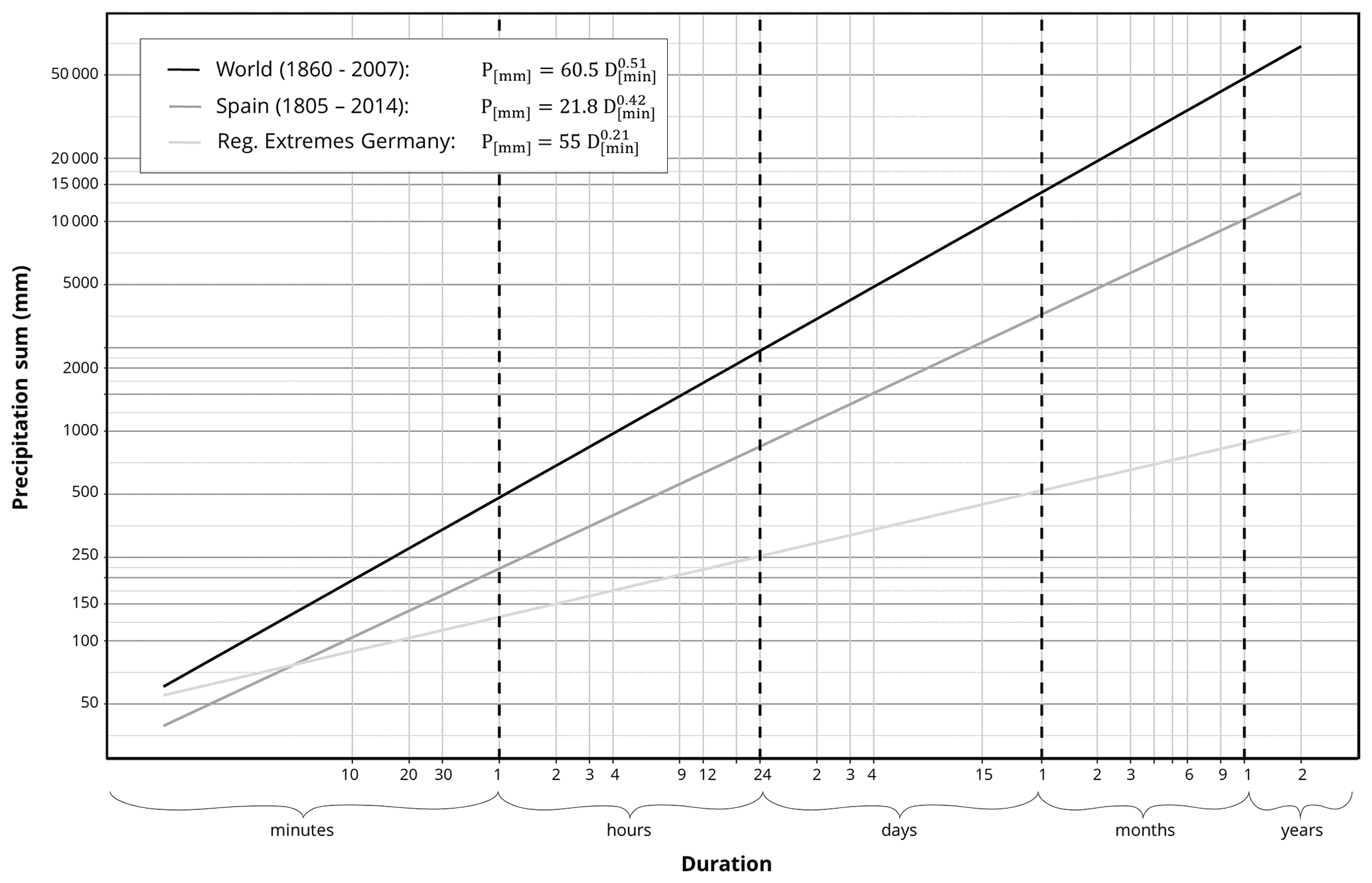
Figure 1 Scaling relationships of extreme (record) precipitation values for different durations based on worldwide data (World Meteorological Organization, 1994; NWS, 2017; Gonzalez and Bech, 2017), Spanish rain gauge data (Gonzalez and Bech, 2017), and a regional analysis of eastern Germany (Dyck and Peschke, 1995).

Several studies examined the validity of this universal scaling exponent. Galmarini et al. (2004) showed, based on rainfall records observed at several stations in Canada, Australia, and La Réunion, that the single exponent scaling laws exist only for single stations experiencing extremely high precipitation and that the deviation from a scaling law is caused by the intermittency associated with a substantial number of zero precipitation intervals in data. They also showed that the scaling exponent β tends to stay around 0.5 based on the stochastic simulation assuming a point rainfall process composed of the Weibull distributed rainfall depth and a given temporal autocorrelation structure. Zhang et al. (2013) showed that the scaling exponent varies around 0.5 if the vertical moisture flux and rainfall can be modelled by a censored (or truncated) first-order autoregressive process AR(1). However, these works showed the scaling behaviour of maximum rainfall at a single point location and did not investigate maxima observed at different spatial locations.

One of the main obstacles to identify the “true” scaling behaviour of maximum rainfall is that most rainfall is measured from sparse ground gauge networks (Dyck and Peschke, 1995; Papalexiou et al., 2016). Breña-Naranjo et al. (2015) used a satellite-based rainfall product to identify the scaling behaviour of the maximum rainfall across the globe. They showed that the maximum of the areal rainfall averaged over the ∼20 km × ∼20 km data grid has the scaling exponent of ∼0.43, which is similar to that of Jennings (1950). However, the coarse spatial resolution of the satellite data easily misses the small-scale rainfall variability that is closely associated with extreme values, thus the extremes found in the satellite data are lower than expected (Cristiano et al., 2017; Fabry, 1996; Gires et al., 2014; Kim et al., 2019; Peleg et al., 2013, 2018).

In this study, we analyse the rainfall depth–duration relationship for all of Germany based on 16 years of RADKLIM-YW, a reprocessed QPE radar product with 1 km–5 min space–time resolution. We want to answer the following questions regarding the scaling behaviour of the maximum rainfall: (1) does the depth–duration relationship of German extreme rainfall show scale invariant behaviour? If so, or if not, what is the primary reason? (2) Does this relationship vary with regard to the spatial sampling rate? (3) Does it provide any clue to modify the relationship currently applied in practice based on sparse gauge networks? The answers to these questions would be especially intriguing because few studies have so far investigated the scaling behaviour of maximum rainfall based on a rainfall data set with such a high spatiotemporal resolution, long recording period, and large spatial extent as this study did.

2 Data and methods

2.1 Data description

The German National Meteorological Service (DWD) has been running a radar network (currently 17 C-band radars) for almost two decades and provides different rainfall data products. Full coverage of Germany has not yet been reached; however, all neighbouring countries contribute to the rainfall information and the network extension continues on an ongoing basis. One QPE from German radar data is RADOLAN (German: RADar OnLine ANeichung) (Winterrath et al., 2012), which combines ground information of fallen precipitation (rain gauge data) with radar data. Since the quality enhancement of RADOLAN is ongoing without post-correcting previous data, the so-called radar climatology project of the DWD, RADolanKLIMatologie (RADKLIM, Winterrath et al., 2017), has consistently reanalysed the complete radar archive set since 2001 for improved homogeneity despite the originally different processing algorithms. Compared to RADOLAN, RADKLIM has implemented additional algorithms leading to consistently fewer radar artefacts, improved representation of orography, as well as efficient correction of range-dependent path-integrated attenuation at longer timescales (Kreklow et al., 2019). Whereas RADOLAN is not well suited for climatological applications with aggregated precipitation statistics, RADKLIM is a promising data set for these climatological applications. The RADKLIM product is available in the following two versions with around 392 128 filled pixels within the German borders: (1) RADKLIM-RW is an hourly precipitation product resulting from radar-based precipitation estimates that are calibrated with ground stations (Winterrath et al., 2018a), which was validated by several studies such as Lengfeld et al. (2019) and (2) RADKLIM-YW (Winterrath et al., 2018b) is a 5 min product resulting from a correction or factoring of the DWD's 5 min product RADOLAN-RY (rainfall estimate after basic quality correction and refined z–R relationship) with the help of RADKLIM-RW on a sequential hourly base. The RADKLIM-YW version 2017.002 was used in this study because it has the high temporal resolution necessary for the analysis. This release is in its third version and covers the years 2001 to 2018. In order to compare with another study at our institute, only years 2001 to 2016 have been used for this study. The YW product covers the area composed of 1100×900 px with a spatial resolution of 1 km (improved compared to former version of RADOLAN). Remaining weaknesses of RADKLIM (as outlined in Kreklow et al., 2019) are a greater number of missing values compared to RADOLAN as well as an underestimation of high intensity rainfall because of spatial averaging and rainfall-induced attenuation of the radar beam.

The data are available as one layer for each time step. Since not all raster pixels are with values (only around half of the values lay within the borders of Germany), the spatial data were converted to time series for quicker processing. The data contain missing values (NaNs) of the following two types: (1) NaNs due to changes and ongoing radar network extension. This mainly affects areas near the border of eastern, northern, and southern Germany. Data in some areas are only available from 2014 onwards. (2) Some locations of raster pixels respectively, have NaNs potentially due to malfunction of the radar or general (radar) errors. Figure 2 shows the proportion of the NaNs of the time series developed for each of the pixels. The visible cones display the individual radar coverage; the overlapping areas of the radar cones have better data coverage than the areas without overlapping.

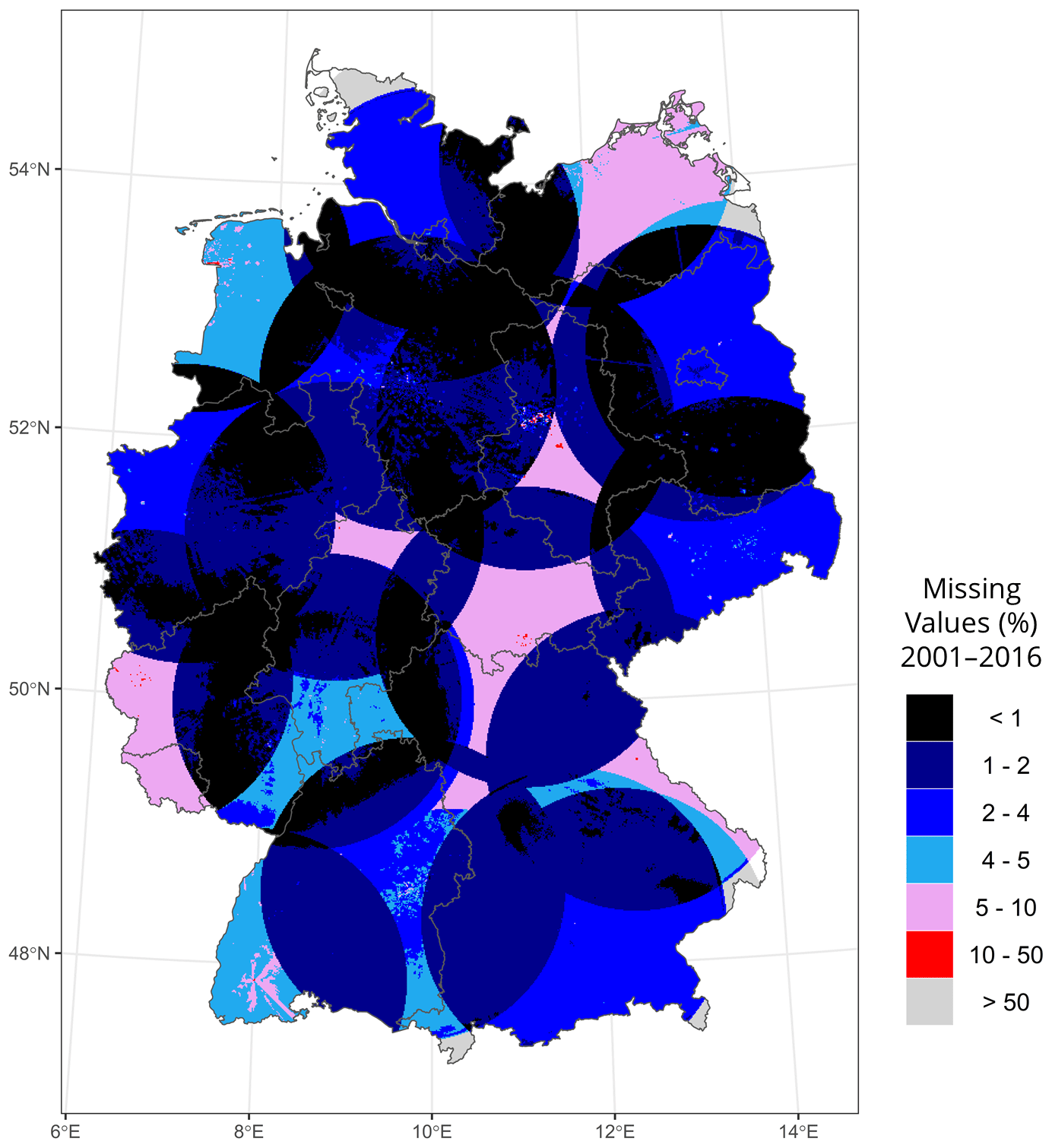
Figure 2 Spatial distribution of the proportion of NaNs (in %) for each pixel of the QPE RADKLIM-YW from 2001–2016. The German boundary is obtained from the GADM Global Administrative Database (Hijmans et al., 2018).

It is hard to handle NaNs in highly episodic geophysical events such as rainfall. We chose to not do any data interpolation, since the consequence of imputing potentially too high extreme values is more severe and uncertain for our study than missing extreme values.

2.2 Depth–duration relationships

Maximum rainfall values for each duration τ between 2001–2016 were calculated with rolling sums applied over moving windows using the R-package Rcpp-Roll (Ushey, 2018). Time windows of up to 3 d were chosen for the analysis, with special focus on the sub-hourly and sub-daily durations. The records may include non-rainfall data and thus do not imply continuous precipitation for the period considered. Values were not aggregated spatially, since this usually reduces the maximum intensity values (Cristiano et al., 2018).

First, the extreme values for each pixel and duration $M_{\max }^{\mathit{\tau },\mathrm{pixel}}$ are calculated. Afterwards, the overall maxima for all of Germany for each $\mathit{\tau }(M_{\max }^{\left(\mathit{\tau }\right)}$) is extracted from these calculated extreme values. Based on these results, the depth–duration relationships can be developed for each pixel as well as for all of Germany.

2.3 K-means clustering of depth–duration relationships

The depth–duration relationships ($M_{\max }^{\mathit{\tau },\mathrm{pixel}}$ vs. τ) for each pixel derived from Sect. 2.2 are individually clustered with the K-means clustering algorithm (Scott and Knott, 1974). “Erroneous” pixels (i.e. having NaNs as resulting maxima) were excluded from the cluster process in order to avoid disturbances. The data were rescaled to make the characteristics more comparable with each other. If the number of clusters is not predefined, it can be identified by drawing an elbow chart. For different numbers of clusters K, the measure of the variability of the observations within each cluster (total within-cluster sum of squares; y axis) is calculated and the curve should bend like an elbow at the optimal value. Since the algorithm did not suggest a number of clusters, we chose six clusters for a sufficiently detailed analysis since it gave consistent results when repeating the automatic algorithm for several times (each time the algorithm clusters slightly differently).

3 Results and discussion

3.1 Scaling behaviour for all of Germany

Figure 3 shows the maximum depth–duration relationship for all of Germany that was derived from the QPE radar data (dots). The same relationship based on the ground gauge network (empty triangles) and the global precipitation extremes (filled triangles) are shown for reference. The rain gauge-based values clearly follow a scaling relationship with a slope that is different in comparison to world extremes. Radar-based maxima for the shorter duration from 2001 to 2016 do not cover all sub-daily extremes but exceed observed ones from the 1 d durations as well as for one sub-daily value. In Fig. 3, a “plateau” is visible between around 35 min up to 18 h, indicating a “one event” effect at 35 min, potentially from an extreme rainfall event in this period. Overall, a scaling behaviour can be observed at sub-hourly durations with a scaling component of around 0.65 even though the maxima are observed rather randomly across all of Germany as indicated by the map showing the location of maximum rainfall. This result implies that even though the location of extreme rainfall is different, the maximum rainfall may exhibit smooth scaling behaviour if the rainfall generation mechanism is similar. As mentioned in the data quality description, it is possible that these sub-hourly values do not represent the true extremes across Germany for 2001–2016, since radar-based measurements at fine timescales are highly sensitive to the effects of averaging. Between 25 min and 16 h, maximum values are calculated for a location at the border of Hesse and Bavaria on 25 August 2006. An extreme event around 30 September 2003 around Berlin comprised the maximum depth–duration relationship at between 18 h and 2 d durations. Weak scaling behaviour existed in the regime at 18 h and 3 d durations with the scaling exponent of 0.20.

Figure 3 Overview of maximum rainfall records in Germany. Chart: maximum depth–duration relationship of rainfall records based on QPE RADKLIM-YW (data of this study) (blue dots) and as reference the relationships based on the German ground network (Rudolf and Rapp, 2003; DWA, 2015; DWD, 2020) (non-filled triangles) and the global precipitation extremes (World Meteorological Organization, 1994; NWS, 2017). Map: locations of rainfall maxima (based on QPE RADKLIM-YW) for the considered duration.

All locations of maxima and the corresponding dates of occurrence are provided in Table 1.

Table 1 Rainfall records for different duration from RADKLIM-YW for 2001–2016 with corresponding locations.

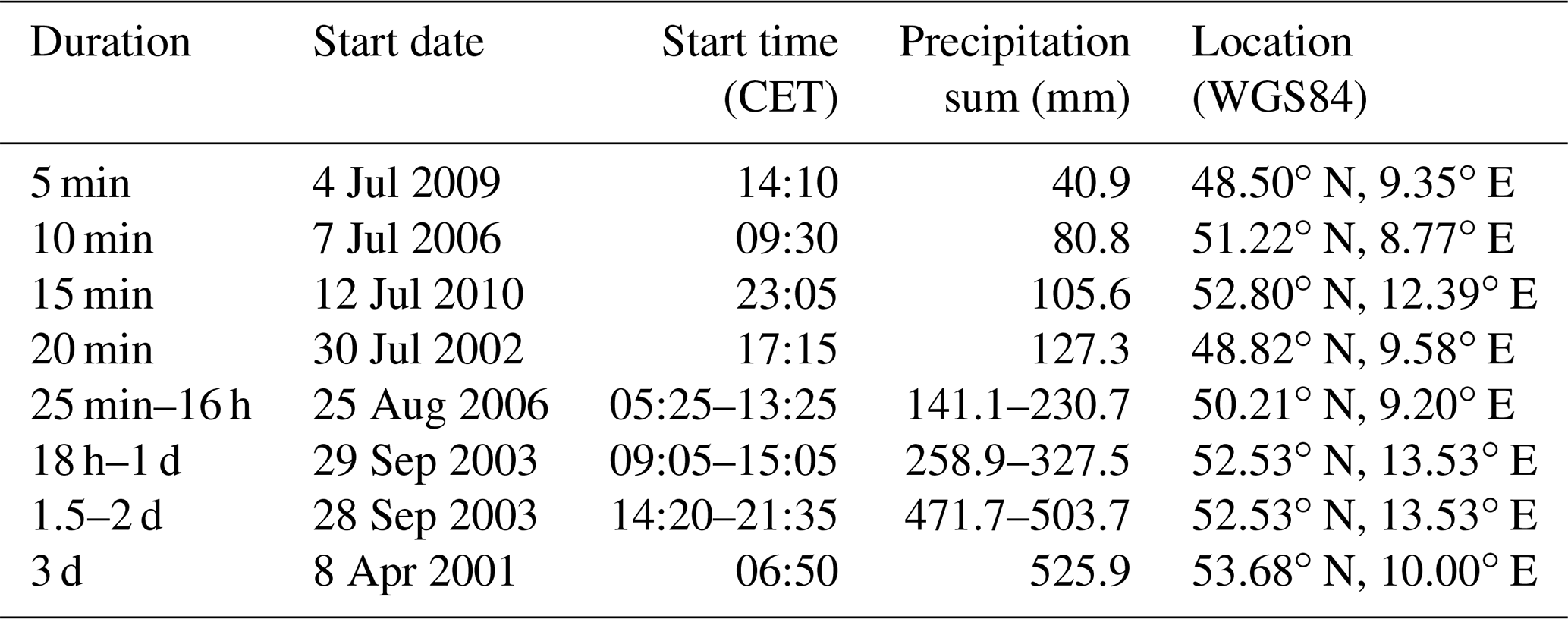
Maxima of 25 min–16 h as well as from 18 h–2 d correspond to the same location and date and are thus summarised.

3.2 Scaling behaviour for all of Germany for high-quantile rainfall

High rainfall values obtained from radar data are associated with especially great uncertainty. Thus, we also investigated the scaling behaviour of high-quantile rainfall values. Figure 4 shows the maximum depth–duration relationship of several quantiles: 0.99999, 0.9999, 0.999, and 0.99. The “three-phase regime” from radar maximum values remains relatively stable, however, the “single event” effect between 50 min and 1 d is smoothed out because the degree of inflections in the curve becomes weaker. Lower quantiles thus show a smoother curve rather than the three-phase regime.

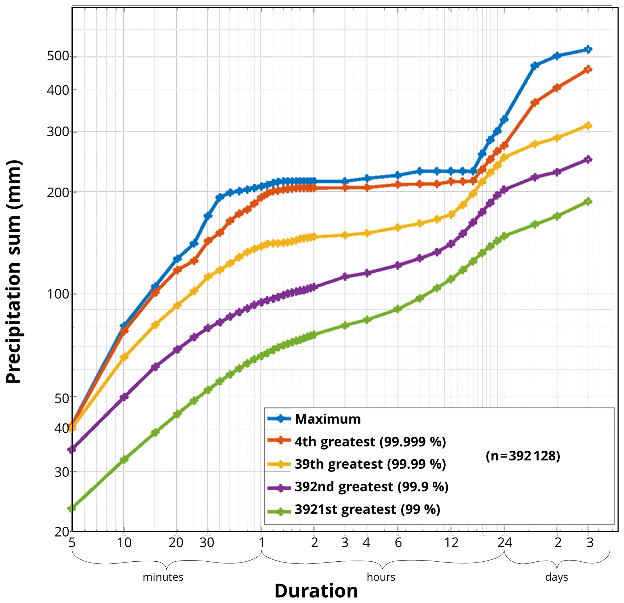
Figure 4 Depth–duration relationships of rainfall values for all of Germany based on QPE RADKLIM-YW for 2001–2016 from maximum values down to the 3921st greatest per duration.

Figure 5 shows the location the high quantile rainfall. The colour of the circles represents the different rainfall durations. It shows that at the highest considered quantile (0.99999) multiple maxima appear at similar locations, potentially referring to the same rainfall events, whereas for lower quantiles (e.g. 0.9999 to 0.99), maxima are more spread over Germany and the visible points increase in number. This suggests the reduction of the influence of one single rainfall event on the depth–duration relationship, causing inflection in the curve.

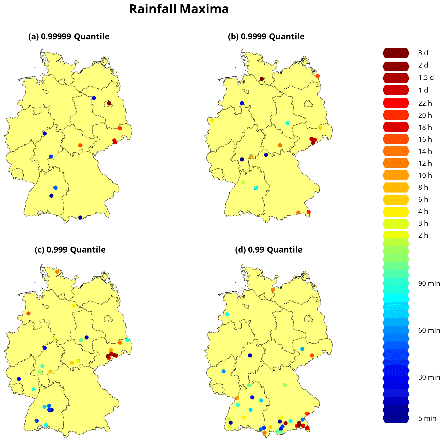
Figure 5 Locations of the 0.99999, 0.9999, 0.999, and 0.99 quantile rainfall with varying durations from 5 min to 3 d. Point colours represent the corresponding rainfall duration, similar for each quantile. Different numbers of data points in panels (a)–(d) result from several data points being at the same location.

Additionally, locations of such high quantile maxima (e.g. 0.99 quantile in Fig. 5) seem to occur predominantly in the wider Alpine region in southern Germany. This suggests that natural rainfall mechanisms are dominating the scaling relationship, such as regional characteristics and meteorological conditions (e.g. orographic lifting or leewards effects). Naturally, one would assume that this heterogeneity in meteorological conditions and rainfall generating mechanisms will reflect regional characteristics and will exhibit some irregular scaling behaviour. Contrary to this conjecture, the curves in Fig. 4 (99.9 % and 99 %) show a quite smooth scaling behaviour.

3.3 Spatial distribution of maximum rainfall

Figure 6 shows the spatial distribution of 5 min, 30 min, 1 h, 6 h, 1 d, and 3 d maximum rainfall over Germany. The red and yellow spots that are spatially distributed in Fig. 6a suggest that 5 min extreme rainfall can happen at any place in Germany. Note that extreme rain occurred also outside the Alpine region at the southern edge of Germany, which suggests that fine-scale extreme rainfall is not necessarily governed by topography. The influence of fine-scale intense rainfall persists until the hourly timescale, as implied by the red and yellow hotspots that are located at similar places in the maps of 5 min, 30 min, and 1 h. The distribution of maxima significantly changes for the duration of 6 h and an interesting pattern emerges in the map of 1 and 3 d duration. These maxima seem to be dominated by single events or single heavy rainfall occurrences. This is especially evident in the 2002 flooding in Saxony (mid-eastern edge) with unprecedented long and heavy rainfall as well as a singular rainfall event in 2014 (narrow aisle in the northwestern area) clearly visible in the maps.

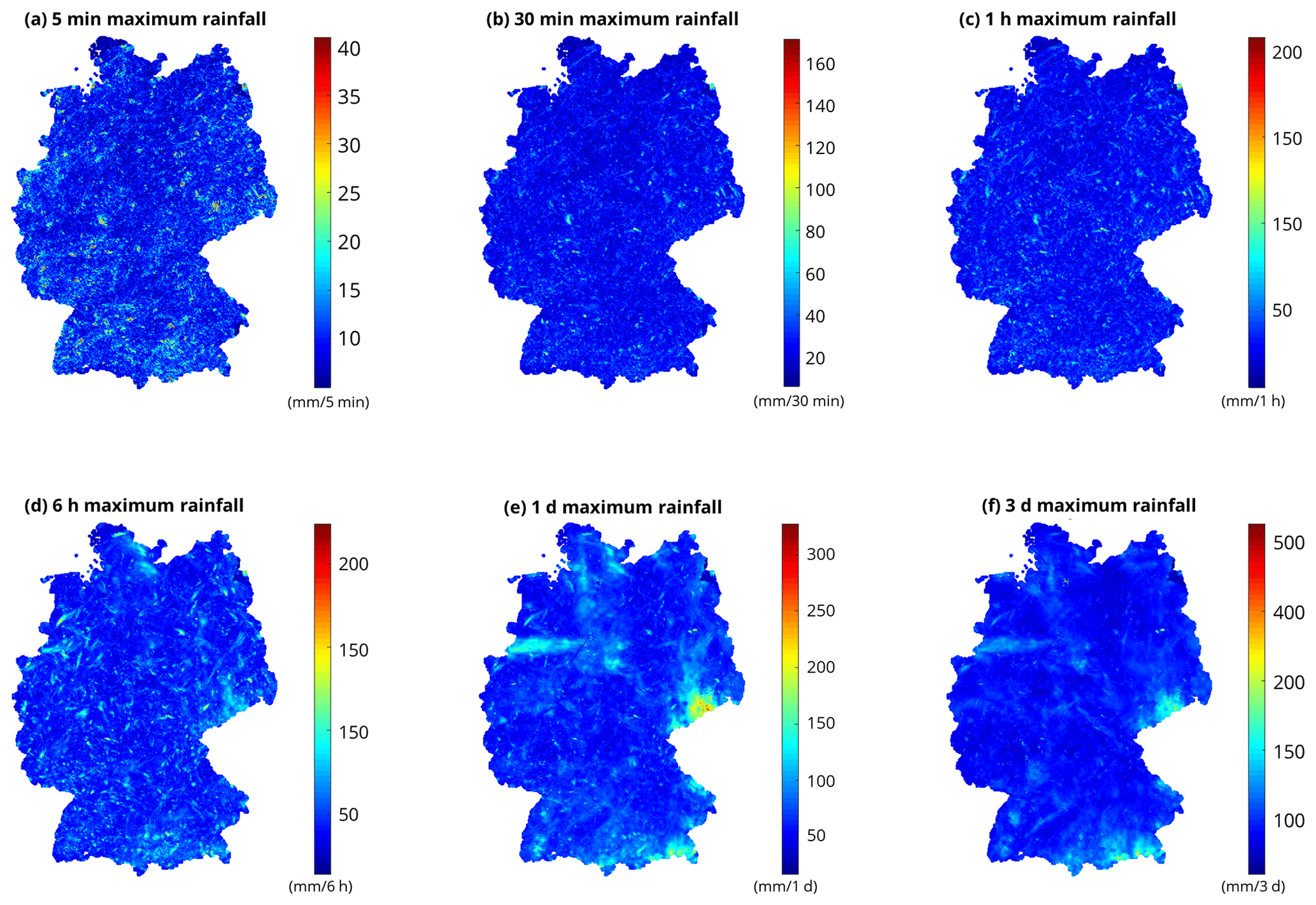
Figure 6 Spatial distribution of the maximum rainfall values retrieved from QPE RADKLIM-YW (2001–2016) for different durations (5 min to 3 d).

3.4 Scaling behaviour at a single point

Figure 7 shows the maximum rainfall–duration relationship of the radar pixels at the major cities of Germany with a single power law (blue) as a reference to see the differences better. Except for Hamburg and Stuttgart, most cities exhibit slight (Hanover, Kiel, Magdeburg, Potsdam, Schwerin, Wiesbaden) to considerable (the remaining cities) deviation from a single power law behaviour. This significant deviation is similar to what was identified by Galmarini et al. (2004) who found that the inflection of the curve is inevitable because of the small (or zero) rainfall observations around a maximum rainfall event. Furthermore, Galmarini et al. (2004) and Zhang et al. (2013) both showed that the maximum rainfall–duration relationship at a given point location follows a smooth and simple power law if the rainfall process can be modelled with a set of simple stochastic processes. Our results imply that natural rainfall processes might significantly deviate from this rather simple assumption; the model framework is also based on very few time series of very different lengths and resolutions.

Figure 7 Depth–duration relationships of rain records for single pixels at rain gauge locations within state capitals of the German federal states.

3.5 Classification of maximum depth–duration relationship

The maximum depth–duration relationships for all pixels within Germany were clustered since Fig. 7 indicated that they might show similar shapes. The K-means clustering algorithm classified the depth–duration relationship into six categories revealing different curve characteristics regarding the curve shapes. Figure 8 shows a categorical map of Germany representing each category with an individual colour. Additionally, depth–duration relationships at 100 randomly chosen grid points from each category are shown with the regression line from category 5 as reference.

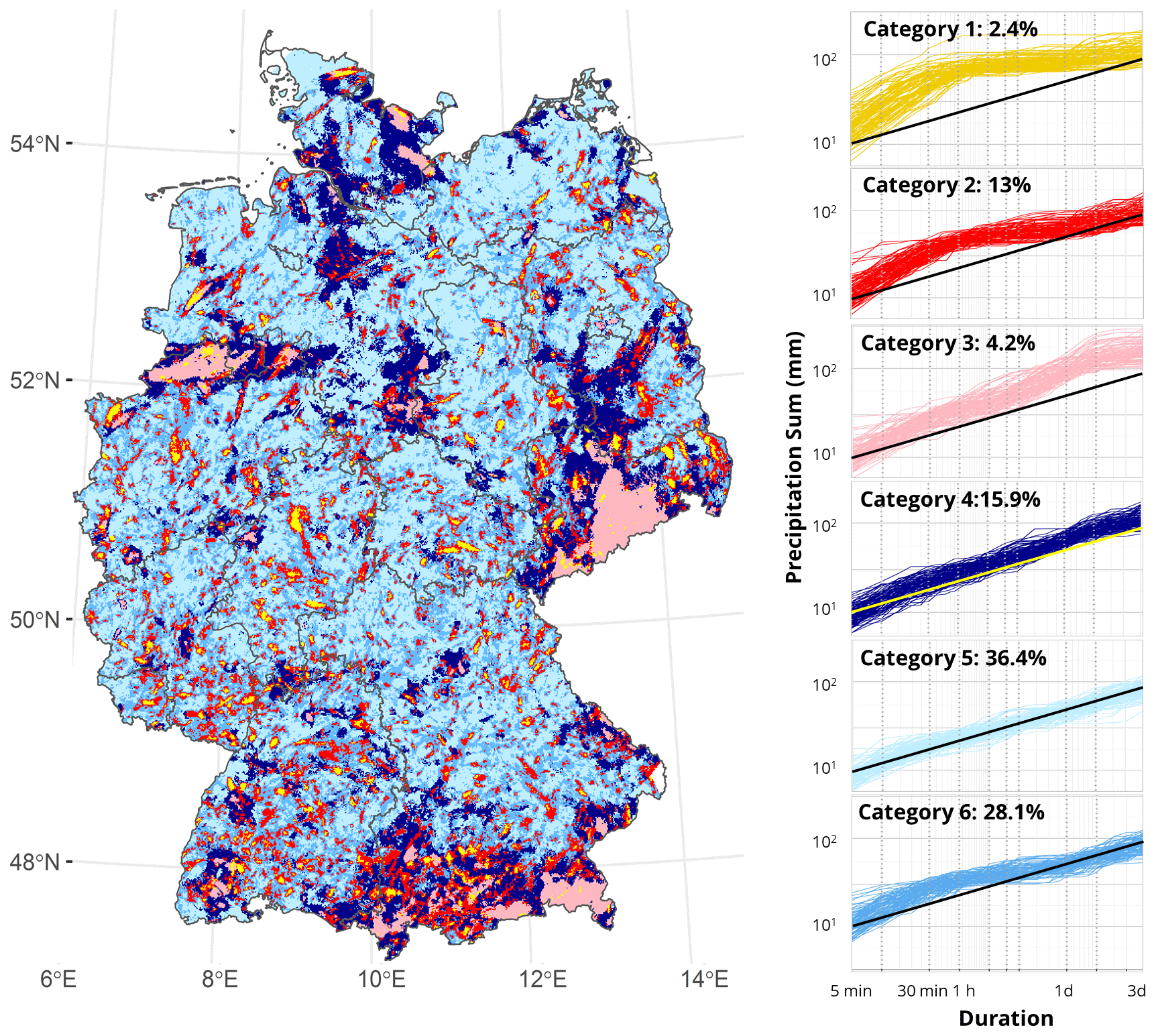
Figure 8 Resulting clusters of the maximum depth–duration relationships of rainfall for all pixels. The left panel shows the spatial distribution of the groups, distinguishable by colour. The corresponding curve shapes of 100 randomly selected radar pixels from each group are displayed on the right side with the same colours as the map.

Pixels belonging to category 1 have the highest rainfall intensities over all scales until 1 d and show a strong inflection at around 1 h, similar to the scaling curve for all of Germany (Fig. 3). The behaviour of the curve between 5 min and 1 h is associated with strong convective rainfall events of around 1 h within the corresponding pixel. Thus, these events are responsible for the high slope at the beginning of the curve. Some curves also show another small inflection between 12 h and 1 d that might correspond to an inter-storm arrival time over which another large event contributes to the positive slope of the curve at durations from 1 d and longer, or simply contributes to the general high intensity of the whole event. Category 1 pixels can be identified as yellow hotspots in Fig. 8 that occur predominantly as smaller areas in the midst of category 2 (red) and partly in category 3 (light pink) pixel clusters. Category 2 pixels (red) have a similar curve shape as those in category 1 and always occur together with category 1 pixels. The curve inflection begins around 30 min and the slope up to 3 d is a little steeper than the slope of category 1. This implies that those locations experienced strong convective patterns of a slightly shorter duration, but potentially longer event durations in general. Most likely, category 1 (event centre) and category 2 (event boundary) pixels experience local convective events, which form in the summer months on warm days with a moist atmosphere. Categories 3 and 4 can be generally associated with large-scale events dominated by regional weather patterns. The three largest clusters in the map can be identified as intense frontal rainfall in August 2002 (Saxony; large cluster in eastern Germany), heavy downpours over Münster in July 2014 (narrow path in the northwestern part), and orographic rainfall in the Alpine region of southern Germany. In category 3, curves show steep slopes of up to 1 d that abruptly end with super-daily duration. This category contributes to the scales between 12 h and 3 d for the curve for all of Germany (Fig. 3). The steep slope at sub-daily duration is because the pixels experienced intense convective storms; however, there was lower intensity at this duration than in categories 1 and 2. Yet, for daily-scale duration they can experience significant amounts of rainfall. Both categories 4 and 5, which compose around 50 % of all pixels, show rough power law behaviour over all scales. Category 4 (dark blue) pixels are mainly at the outer borders of the described larger events as well as adjacent to pixels of categories 1 and 2. Thus, the curves have steep slopes because the corresponding pixels experienced great rainfall. Most pixels belong to category 5 (36 %), showing the smoothest scaling behaviour of all categories. Based on the data set, these regions or locations respectively, have never been hit by any “extreme” extreme event that could have altered the power law behaviour of the depth–duration relationship. The locations of these pixels indicate no spatial pattern and can be seen as a kind of background colour of the map. The last category, category 6, contains similar characteristics as categories 1 to 3 and comprises another 30 % of all pixels. This category represents pixels experiencing common types of convective events with short heavy rainfall sequences on the sub-hourly scale, indicated by a relatively steep slope until 1 h compared to categories 1 and 2. However, these pixels also experience longer rainfall sequences, thus showing an almost three-phase regime as the overall curve for Germany with lower values. The found clusters can be further summarised into three classes. The first class is pixels that experienced very heavy rainfall on a sub-hourly scale (categories 1 and 2) exhibiting steep slopes at sub-hourly scale and mild slope for longer duration. The second class experienced heavy rainfall sequences of up to 1 d (categories 3 and 4). The third type shows power law behaviour over all scales and can be mainly found in category 5. Category 6 simultaneously shows characteristics of classes 1 and 2.

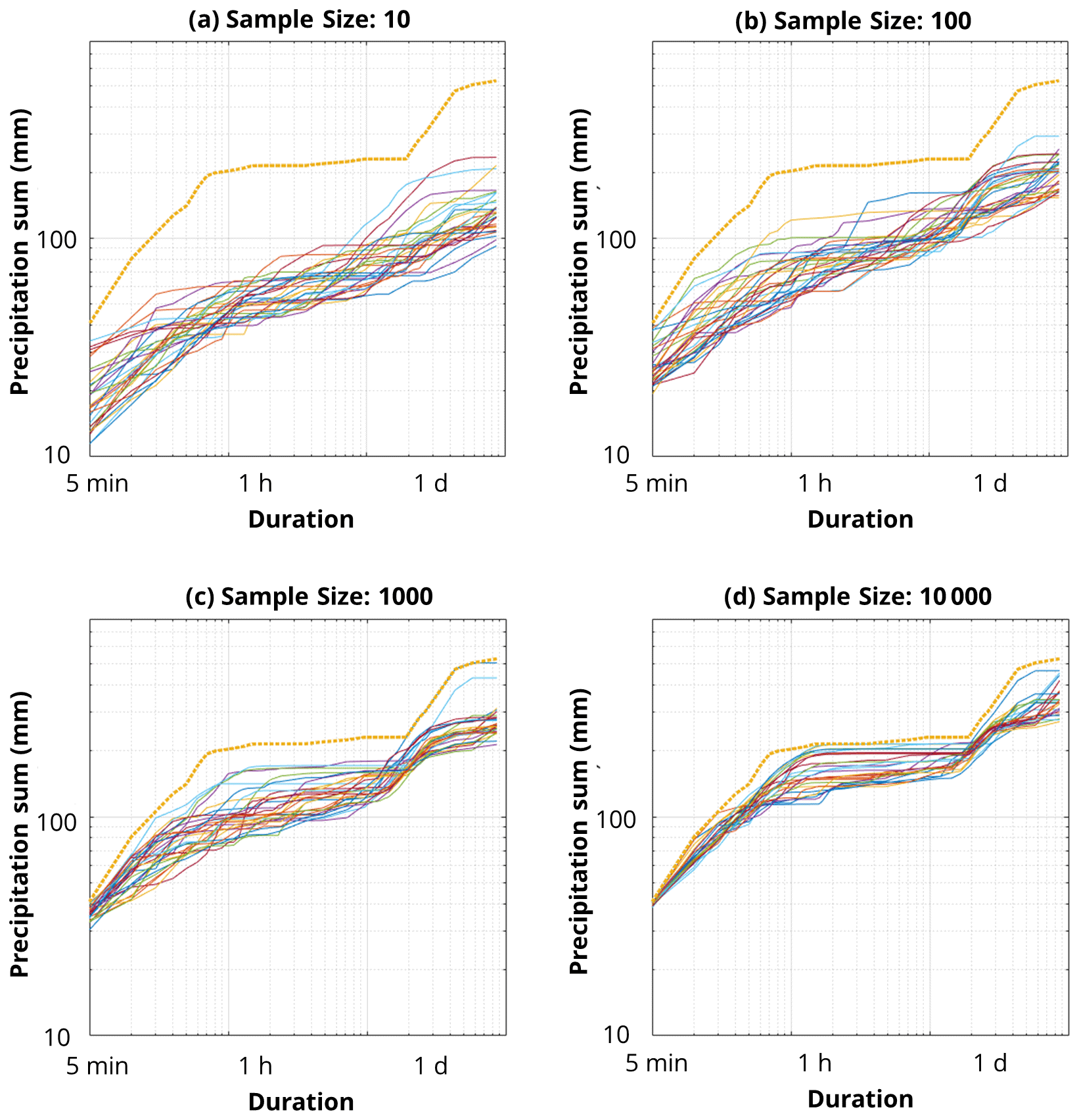
Figure 9 Dependency of maximum depth–duration relationship characteristic on underlying pixel sample size. The maximum rainfall values are derived from (a) 10, (b) 100, (c) 1000, and (d) 10 000 random pixels from all considered pixels (n=392 128) within Germany. For each sample size, 30 ensembles are displayed and compared to the overall maximum curve from Figs. 3 and 4 (yellow top line).

3.6 Sensitivity of scaling behaviour to ground gauge network density

An important message from Sects. 3.4 and 3.5 is that the depth–duration relationship at a given point varies location by location based on the occurred rainstorms. This implies that the maximum depth–duration relationship over the entire study area, which is fundamentally the process of the superposition of these various relationships and the picking up of the very maximum values at each duration, may vary with regard to density and spatial formation of ground gauge networks (compare with previous section). For this reason, we investigated how the depth–duration relationship would vary with regard to a different number of sampling pixels. Figure 9 shows the result corresponding to the pixel sample size of 10, 100, 1000, and 10 000. For each of the cases, 30 ensembles of random pixel sampling were performed. For each of the plots, the maximum depth–duration relationship based on all radar pixels (n=392 128) was shown for reference. Clear and smooth scaling behaviours are identified when the pixel sample size is 10 and 100, but the smooth scaling behaviours are lost when including more major rainfall events that formed the original maximum depth–duration relationship. This emphasises that the number of rain gauges in a network is extremely relevant in order to adequately capture rainfall extremes. It is of note that most scaling relationships of the past including Jennings (1950) were based on the measurements of the ground gauge network. The station density was used as “best we could get” and was not tested against a smaller set of stations, as obviously including all reliable extremes improves the relationship. This might work for the Jennings curve, as a global scale (space and time) can make up for a limit in spatial resolution. However, regional scaling suffers from the limited spatial extent, which cannot be completely balanced by a denser network or radar data.

4 Conclusions

A thorough understanding on the scaling behaviour of the depth–duration relationship of extreme precipitation has been limited because its high spatiotemporal variability cannot be fully captured by a measurement network composed of limited number of ground gauges. This study tried to overcome this limitation by using the radar quantitative precipitation estimate (QPE) rainfall product RADKLIM-YW. The radar QPE enabled clear identification and explanation of the characteristics of the different scaling regimes of extreme rainfall depth–duration relationships. The maximum depth–duration relationship derived from radar data did not show clear scaling behaviour compared to one based on gauge data from longer time series, but exhibited a three-phase regime with a high slope at the duration smaller than 1 h, a plateau at the duration between 1 h and 1 d, and a low slope at the duration greater than 1 d. The relationship was developed based on only a few extreme rainfall events, which dominated the shape of the curve and this changed when examining quantiles of pixel maxima. The depth–duration relationship of lower quantile rainfall (e.g. 99th percentile) showed a smooth scaling behaviour and the rainfall events contributing to the curve sparsely occurred at various locations of Germany. This implies that the modest extreme rainfall events are less sensitive to the random effects of a limited period (under sampling) and may even share common atmospheric conditions of rainfall generation regardless of pixel location in a limited region like Germany. The rainfall depth–duration relationship at a single radar pixel did not show clear power law behaviour either. The shape of the curve was governed by the temporal structure of the extreme rainfall events at the pixel location. The point-wise clustering of depth–duration relationships revealed three classes of scaling behaviour: (a) linear scaling over all durations, as well as inflections at (b) 1 h and (c) 1 d, which shows the influence of small convective pixels as well as large-scale weather patterns on the depth–duration relationship. The scaling behaviour thus can be significantly different for each pixel because the rainfall characteristics for each pixel are very different as well. Given that the extreme rainfall depth–duration relationship over a region is a process of overlapping the relationships observed at various pixel locations and picking up the highest rainfall values at each duration, the result implies that the depth–duration relationship of extreme rainfall can significantly deviate from power law behaviour. With longer available time series of radar in the future, the deviation can be further investigated and tested. Also, the known issue of rainfall extreme underestimation by RADKLIM-YW and the potential impact on the results need further evaluation.