Downsizing parameter ensembles for simulations of rare floods

For extreme-flood estimation, simulation-based approaches represent an interesting alternative to purely statistical approaches, particularly if hydrograph shapes are required. Such simulation-based methods are adapted within continuous simulation frameworks that rely on statistical analyses of continuous streamflow time series derived from a hydrological model fed with long precipitation time series. These frameworks are, however, affected by high computational demands, particularly if floods with return periods > 1000 years are of interest or if modelling uncertainty due to different sources (meteorological input or hydrological model) is to be quantified. Here, we propose three methods for reducing the computational requirements for the hydrological simulations for extreme-flood estimation so that long streamflow time series can be analysed at a reduced computational cost. These methods rely on simulation of annual maxima and on analysing their simulated range to downsize the hydrological parameter ensemble to a small number suitable for continuous simulation frameworks. The methods are tested in a Swiss catchment with 10 000 years of synthetic streamflow data simulated thanks to a weather generator. Our results demonstrate the reliability of the proposed downsizing methods for robust simulations of rare floods with uncertainty. The methods are readily transferable to other situations where ensemble simulations are needed.

1 Introduction

The quantification of extreme floods and associated return periods remains a key issue for flood hazard management (Kochanek et al., 2014). Extreme-value analysis was largely developed in this field for the estimation of flood return periods (Katz et al., 2002); corresponding methods have been recently extended to bivariate approaches that assign probabilities jointly to flood peaks and flood volumes (Favre et al., 2004; De Michele et al., 2005; Brunner et al., 2016) and to trivariate approaches to assign probabilities jointly to flood peaks, volume and duration (Zhang and Singh Vijay, 2007); for a review of this field, see the work of Graler et al. (2013).

Most modern applications, however, require the estimation of not only extreme peak flow, associated flood volumes and duration but also of hydrograph shapes, in particular in the context of reservoir design or for safety checks of hydraulic infrastructure (Kochanek et al., 2014; Gaál et al., 2015; Zeimetz et al., 2018). The key is thus the construction of design hydrographs with different shapes, peak flows and volumes, with a corresponding probability of occurrence. Such approaches can be roughly classified into methods that identify the shape of these design hydrographs based on observed data (Mediero et al., 2010) or based on theoretical considerations (unit hydrographs) (Brunner et al., 2017) and regionalization (Tung et al., 1997; Brunner et al., 2018a) or methods that rely on streamflow simulations (Arnaud and Lavabre, 2002; Kuchment and Gelfan, 2011; Paquet et al., 2013).

Simulation-based methods for design or extreme-flood estimation have a long history in hydrology (for a review see Boughton and Droop, 2003) and started with the classical event-based simulation with selected design storms (Eagleson, 1972; Chow et al., 1988; American Society of Civil Engineers, 1996). Those event-based methods are based on the concept that the design storm and flood have the same return period. Moreover, as they usually do not simulate antecedent conditions prior to the event and do not account explicitly for storm patterns (duration, spatial and temporal variability), they may yield biased flood frequency distributions (Viglione and Blöschl, 2009; Grimaldi et al., 2012a). Although some modern extensions of this event-based concept account for variable initial conditions prior to the event through sensitivity tests (Filipova et al., 2019), most of the work using event-based simulations assume default initial conditions. Indeed, such event-based simulation is still in use, in particular in the context of probable maximum flood (PMF) estimation based on probable maximum precipitation (PMP) (Beauchamp et al., 2013; Gangrade et al., 2019).

Modern extensions of this approach, however, use continuous hydrological modelling for design flood estimation to generate either (i) a range of initial conditions for use in combination with design or randomly drawn storms (Paquet et al., 2013; Zeimetz et al., 2018) or (ii) long discharge time series from long observed-precipitation records or from synthetic precipitation time series obtained with a weather generator (Calver and Lamb, 1995; Cameron et al., 2000; Blazkova and Beven, 2004; Hoes and Nelen, 2005; Winter et al., 2019). The above approach (ii) is computationally intensive, especially if long time series are to be simulated using ensembles of hydrological parameter sets or if very high return periods (>1000 years) have to be robustly estimated. But in exchange, return period analysis is straightforward for simulated peak flows or volumes. Full hydrographs for risk analysis are then obtained by either selecting a range of simulated extreme events or by scaling up an estimated synthetic design hydrograph by quantiles of extreme peak and volume estimated using frequency analysis (Pramanik et al., 2010; Serinaldi and Grimaldi, 2011).

These fully continuous simulation schemes are particularly useful for studies where recorded discharge time series are too short for extreme-flood analysis (Lamb et al., 2016; Evin et al., 2018). Although such an approach is based entirely on a continuous hydrological simulation, it is noteworthy that such a fully continuous approach might still be considered to be “semi-continuous” from a hydraulic perspective since corresponding studies often lack the final hydraulic routing step along the floodway (Grimaldi et al., 2013). For clarity, we therefore use the term “continuous hydrological simulation scheme” to distinguish it from the abovementioned hydraulic approach. These continuous hydrological simulation frameworks are still rare for time series ≥ 100 years due to heavy computational requirements (Grimaldi et al., 2013). An example is the work of Arnaud and Lavabre (2002), who use a continuous simulation framework to generate an ensemble of possible extreme hydrographs, which are then used as individual scenarios for hazard management. Another option is to summarize all simulated flood hydrographs into probability distributions for peak flow and flood volume (Gabriel-Martin et al., 2019).

High computational power is particularly needed in order to provide estimations for high to extreme return periods (up to 1000 years and higher) required for safety-related studies or for hydrological-hazard management. For such rare events, the large number of simulations in fully continuous frameworks can easily become prohibitive, in particular if the framework should also account for different sources of modelling uncertainty, such as input uncertainty (different weather generators) or the uncertainty in the hydrological model itself, which is often incorporated into the model parameter sets (using distribution of model parameters rather than a single best set) (Cameron et al., 1999). Using multiple parameter sets for a hydrological model is justified by the parameter equifinality (Beven and Freer, 2001; Sikorska and Seibert, 2018b). It has also been found that the model parameter uncertainty comprises important uncertainty sources in design floods that are based upon hydrological simulations (Brunner and Sikorska-Senoner, 2019). Other important uncertainty sources in hydrological modelling are linked to the calibration (discharge) data, input forcing (precipitation, temperature, evaporation) data and model structure (Sikorska and Renard, 2017; Westerberg et al., 2020).

Studies dealing with modelling or data uncertainties in such continuous simulation frameworks are rare as most previous studies have focused on the uncertainty related to the hydrological-model parameters only (e.g. Blazkova and Beven, 2002, 2004; Cameron et al., 1999). In addition to the uncertainties from seven hydrological-model parameters, Arnaud et al. (2017) investigated how the uncertainty related to six rainfall generator parameters propagates through the simulation framework using more than 1000 French basins with hydrological observation series of 40 years (median over all basins) and several hundreds of replicates. In their study they found that the uncertainty in the rainfall generator dominates the uncertainty in the simulated extreme-flood quantiles. With the exception of the work of Arnaud et al. (2017) using a simplified hydrological model, studies that deal with meteorological- and hydrological-modelling uncertainty in fully continuous simulation frameworks are currently missing. This is despite the fact that recent improvements in computational power with cluster and cloud computing theoretically open up the unlimited possibility of analysing different combinations of meteorological scenarios and parameter sets of a hydrological model within such ensemble-based simulation frameworks. Yet, computational constraints of hydrological models, especially at a high temporal resolution (sub-daily or hourly), and data storage still remain bounding factors for simulation of long time series or for simulation of extreme floods with high return periods (up to 10 000 years).

Accordingly, for settings where full hydrological–hydraulic models are used for continuous simulation, some pre-selection of hydro-meteorological scenarios is often needed, particularly for computationally demanding complex hydrological or hydraulic models. How this selection should be completed, i.e. based on which quantitative criteria, remains unclear. The meteorological scenarios have the particularity that all scenarios generated with the same weather generator present different but equally likely realizations of the assumed climate condition; in other words, they represent the natural variability in the climate. Reducing the number of meteorological-input scenarios is not possible without simulating them with a hydrological model first as long as the continuous simulation scheme is of interest, i.e. if full time series are to be analysed without the possibility of extracting single events. This is due to the non-linear response of any hydrological model to meteorological input (scenario), which translates into hydrological scenarios with different statistical properties, albeit resulting from an ensemble of input scenarios having the same statistical properties.

We are therefore essentially left with finding ways to reduce at least the computational requirements associated with hydrological-model parameter uncertainty, apart from reducing the length of time series, which for analysis of extremes, is an unattractive option. Accordingly, in this work, we propose an assessment of different data-based methods to select a reduced-size ensemble of hydrological-model parameters for the use within a continuous simulation, ensemble-based hydro-meteorological framework. Our specific research questions are as follows. (1) How can we downsize (reduce) the hydrological-model parameter ensembles for simulation of rare floods so that the variability and the range of the full ensemble is preserved as closely as possible? (2) Can such a reduced hydrological-model parameter ensemble be assumed to be reliable for the simulation of rare floods during the reference period (used for parameter ensemble downsizing) as well as during an independent validation period? (3) Which metrics would be suitable to assess the performance of such a reduced hydrological-model parameter ensemble against the reference (full) ensemble? Specifically, three different methods of reducing a full hydrological-modelling parameter ensemble to a handful of parameter sets are proposed and tested for deriving the uncertainty ranges of simulated rare flood events (up to 10 000 years return period). All three methods rely on simulation of annual maxima and are tested on continuous synthetic data (simulated with a hydrological model) of 10 000 years. Using synthetic instead of observed data is important here as only recently Brunner et al. (2018b) have shown that the record length is one of the most important sources of uncertainty in design floods. Hence, using a simulation setting with synthetic data as a start for our analysis enables us (i) to provide long enough simulation periods for rare-flood analysis with return periods ≥ 100 years and (ii) to be able to focus entirely on the uncertainty in the hydrological response, while other uncertainty sources of a hydrological model (due to model calibration) are not explicitly considered. Note that way the hydrological model is calibrated lies outside of the scope of this paper. The principal idea underlying these selection methods is that the downsizing of the ensemble of hydrological-model parameters may be performed with a reduced length of input time series that is much shorter than the full simulation time frame and that then can be applied to the full time window for analysis of rare floods (up to return periods of 1000 years or more).

2 Methods

2.1 Study framework and objectives

The focus of this study is a fully continuous hydro-meteorological ensemble-based simulation framework for estimation of rare floods. The underlying streamflow time series ensemble is built based on meteorological scenarios and multiple hydrological-model runs using a number of calibrated model parameter sets. A meteorological scenario represents a single realization from a stochastic weather generator with constant model parameters. These meteorological scenarios are equally likely model realizations that differ in the precipitation and temperature patterns, and together they represent the natural variability in the climate (and not the model uncertainty in a weather generator). These realizations are then used as inputs into a hydrological model to simulate the hydrological response. To account for hydrological-modelling uncertainty, a range of different hydrological-model parameter sets is used for each meteorological scenario. These two sources of hydrological variability then accumulate along the modelling chain and can be represented as an ensemble of possible hydrological responses (Fig. 1).

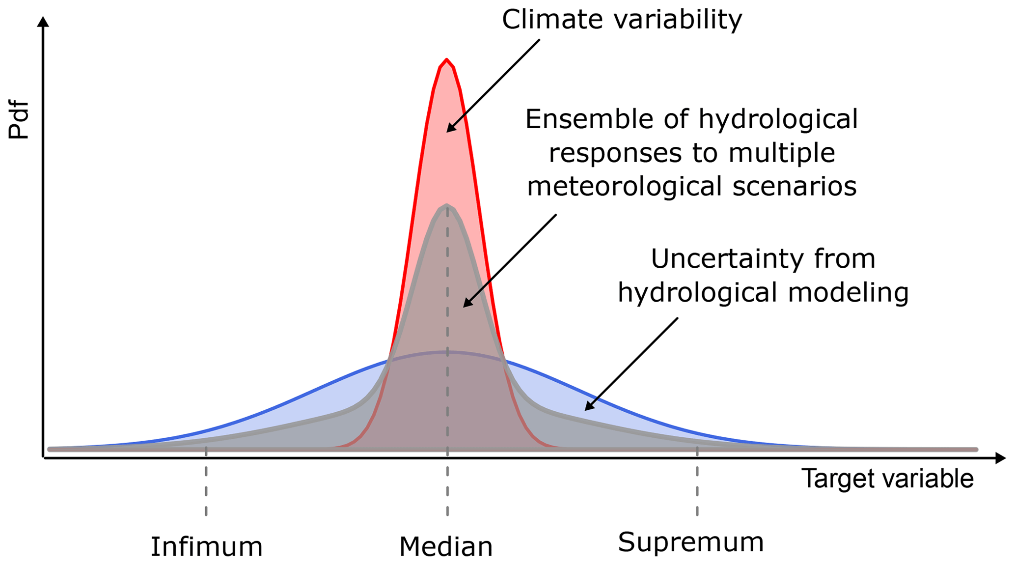
Figure 1 Framework overview. The infimum and supremum refer to the largest interval bounding the ensemble simulation from below and the smallest interval bounding it from above.

Within such a defined framework we first want to understand how variable the hydrological response simulation is and, second, develop methods to downsize the hydrological-model parameter ensemble to a smaller subset that could be dealt with within such a modelling chain for rare-flood simulations. This subset should represent the entire range of variability in the hydrological response but with little computational effort and should also be transferable to independent time periods. Hereafter, we call this subset the representative parameter ensemble.

Downsizing of the ensemble of hydrological-model parameters is particularly needed if (i) the probability distribution of the parameter sets is unknown because parameter sets result from independent calibrations or regionalization approaches, and only a limited number of sets can be run with the hydrological model, or (ii) the distribution is known (i.e. estimated from data), but due to time-consuming simulations it is not possible to run the hydrological model for a full ensemble of multiple meteorological scenarios.

The question of how many parameter sets are needed to cover most of the simulation range is important. However, here we set this value to a constant number and rather test different selection approaches. Hence, for the purpose of our work, we furthermore would like this representative parameter ensemble to be composed of only three sets, which should be representative of a lower (infimum), a middle (median) and an upper (supremum) interval of the full hydrological ensemble (Fig. 1). These intervals, together, should enable the construction of predictive intervals for rare-flood estimates that represent the full variability range of all ensemble members. The infimum (from the Latin – smallest) and supremum (from the Latin – largest) refer to the greatest lower bound and the least upper bound (Hazewinkel, 1994), i.e. the largest interval bounding the ensemble from below, here 5 %, and the smallest interval bounding it from above, here 95 %. Thus, the representative band should correspond to 90% predictive bands of a target variable. The choice of infimum and supremum is favourable over the maximum and minimum as the latter would imply a complete hydrological-model parameter ensemble range, whereas here we use the terms to describe the range of a certain ensemble.

The key challenge for such a downsizing is the fact that we would like to select hydrological-model parameter sets (i.e. select in the parameter space) but based on how representative the corresponding simulations are in the model response space. Moreover, the downsized ensemble should not only be representative of simulated time periods but also be transferable to independent time periods. The first question to answer is which model response space the selection should focus on. In the context of rare-flood estimation, focusing on the frequency distribution of annual maxima (AMs) is a natural choice; we thus propose to use the representation of AMs sorted by their magnitudes (i.e. frequency space) as the reference model response space for parameter selection.

The next step is the development of selection methods to select hydrological-model parameter sets that plot into certain locations in the model response space. Given the nonlinear relationship between model parameters and hydrological responses, this selection has to be obtained via a post-modelling approach; i.e. we have to first simulate all parameter sets and then decide which parameter sets fulfil certain selection criteria in the model response space.

For that purpose, we developed three methods, which are based on (a) ranking, (b) quantiling, and (c) clustering, described in detail in Sect. 2.2. The main idea behind all three methods is that the hydrological-parameter set selection is made based on the full ensemble with all hydrological-model simulations but using only a limited simulation period that is much shorter than the time window of full meteorological scenarios used within the simulation framework for which rare floods are to be estimated.

Next, for the purpose of this study, let us define the following variables:

• I is a number of hydrological-model parameter sets available, with i=1, 2, … being a parameter set index.

• θ_i is the ith parameter set of a hydrological model.

• J is a number of annual maxima (years) per hydrological simulation; y=1, 2, … is a year of simulation (index of unsorted annual maxima); and j=1, 2, … is an index of sorted annual maxima.

• X_j is the jth sorted annual maximum, and X_y is the unsorted annual maximum from the year y.

• M is a number of meteorological scenarios considered, with m=1, 2, … being a meteorological scenario index.

• S_m is the mth meteorological scenario.

• H(θ_i|S_m) is the hydrological simulation computed using the ith parameter set of a hydrological model and the mth meteorological scenario.

• $X_{y,i,\mathrm{m}}$ is the annual maximum for the year y extracted from H(θ_i|S_m).

• θ_inf, θ_med and θ_sup are the representative parameter sets of the hydrological model, i.e. infimum, median and supremum that correspond to the intervals named in the same way.

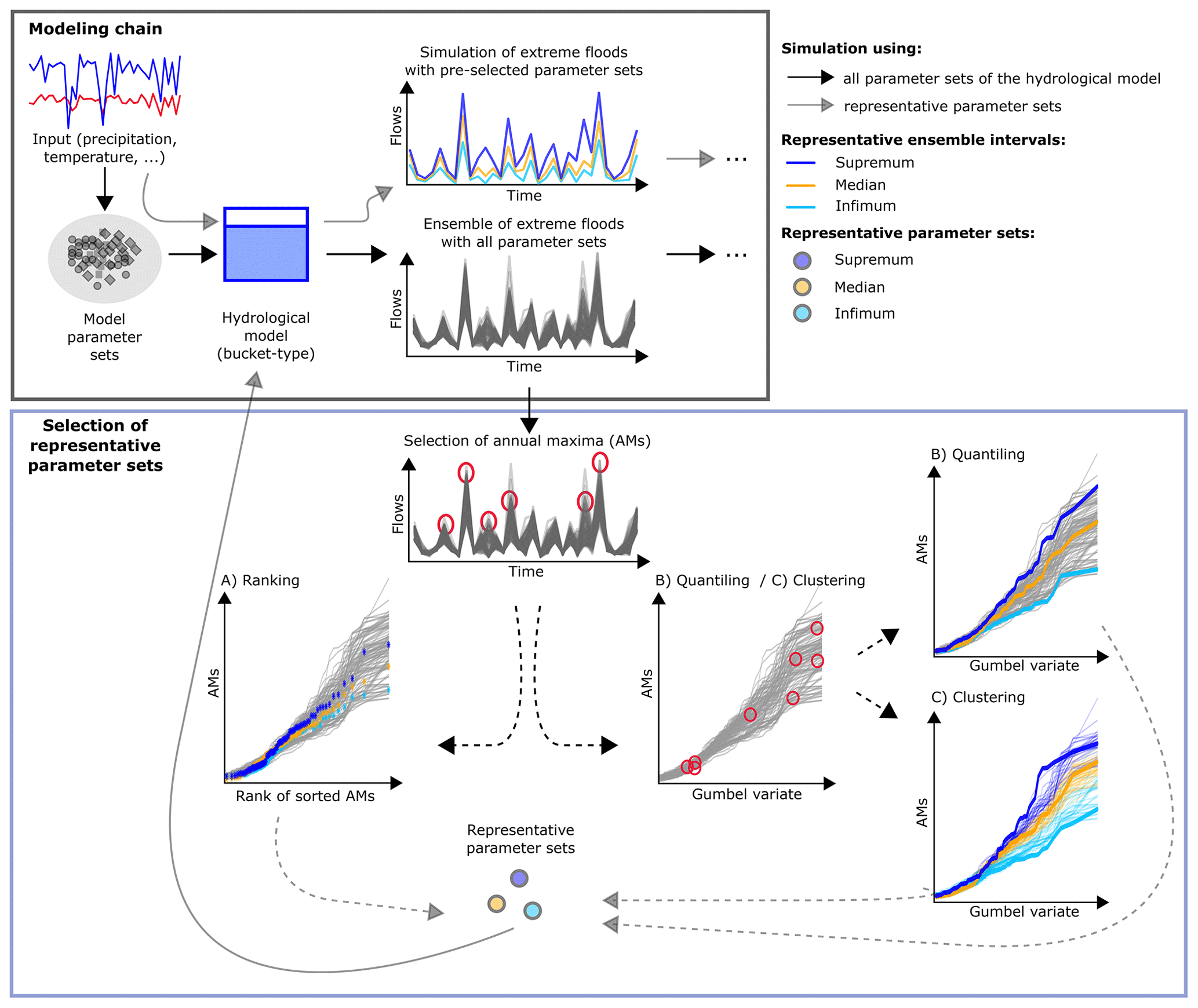
Figure 2 Overview of the modelling chain and the selection methods of the representative parameter sets; (a) delivery of hydrological-simulation ensembles and ensemble ranges; (b) three methods (A–C) proposed for selecting the representative parameter sets based on annual maxima (AMs) marked with red circles.

2.2 Developed methods for selecting the representative parameter sets

For the sake of simplicity, let us choose a single meteorological scenario S_m for now. Using S_m as an input into a hydrological model combined with I parameter sets results in an ensemble of hydrological simulations, $H\left({\mathit{\theta }}_{\mathrm{1},\mathrm{2},\mathrm{\dots }}\right|{\mathit{S}}_{\mathrm{m}})$. Now, the goal is to select a limited number (here three) of hydrological-model parameter sets, i.e. θ_inf, θ_med and θ_sup, from the available pool of I sets (I≫3) based on the simulation of annual maxima (AMs). These AMs are extracted from time series with continuous hydrological simulations, i.e. $H\left({\mathit{\theta }}_{\mathrm{1},\mathrm{2},\mathrm{\dots }}\right|{\mathit{S}}_{\mathrm{m}})$, using a maximum approach that guarantees that the highest peak flow within each calendar year for each hydrological simulation is selected (Fig. 2). This assumption is made to cover the situation when different model realizations (i.e. for i=1, 2, …) lead to different flood events being classified as the largest event within the year. In this case, we ensure that the largest flood event simulated within each yth year and each ith parameter set is selected. This means however that AMs selected for the same year y but with a different hydrological-model parameter set may originate from different flood events and even from a different dominant flood process, e.g. heavy rainfall or intensive snowmelt (Merz and Blöschl, 2003; Sikorska et al., 2015). This could be the case when one hydrological-model parameter set better represents processes driven by the rainfall excess, while others better represent processes driven by the snowmelt dynamics. For simplicity, we do not distinguish events by their different flood genesis and pool all AMs together.

Using the above notations, the selection of representative parameter sets can be summarized as follows.

1. Simulation of continuous streamflow times series: the hydrological model is run with all available I parameter sets of a hydrological model over the simulation period. This gives I different hydrological realizations (simulation ensemble members) covering the same time span.

2. Selection of annual maxima (AMs): for each ith hydrological realization, annual maxima are selected as the highest peak flow within each yth simulation year. This results in a J set of AMs per i hydrological simulation. The selection of AMs is repeated for all I hydrological simulations.

3. Selection of three representative parameter sets based on the simulation of AMs and following on from the three methods detailed below.

2.2.1 Ranking

• a.

  AMs computed from I hydrological simulations (i.e. using I hydrological-model parameter sets) are sorted by their magnitude from the highest to the lowest within each yth simulation year independently (Fig. 2a).

• b.

  For each yth simulation year, AMs which correspond to the 5th, 50th and 95th rank for that year are selected.

• c.

  Parameter sets that correspond to the selected AM ranks are then attributed as 5th, 50th and 95th parameter sets per yth year independently.

• d.

  The parameter sets selected in step (c) are compared over all J simulation years, and the sets which are chosen most often as the 5th, 50th and 95th ranks are retained as the parameter sets θ_R5, θ_R50 and θ_R95 representative of the entire simulation period and for the entire hydrological-simulation ensemble.

2.2.2 Quantiling

• a.

  For each ith hydrological-model parameter set, AMs computed with this parameter set are sorted by their magnitude over the entire simulation period (J years), thus creating the ensemble of sorted AMs simulated with different parameter sets.

• b.

  The 5 %, 50 % and 95 % quantiles of these ensembles are computed at each jth point in the frequency space, resulting in quantiles Q₅, Q₅₀ and Q₉₅ over the entire simulation period (Fig. 2b).

• c.

  Next, for each ith ensemble member, a metric R_MSE is computed such that for each jth point of the ith ensemble member it measures distances from Q₅, Q₅₀ and Q₉₅. This metric is somehow similar to the mean square error and is computed for Q₅₀ as

  $$\begin{array}{}\text{(1)}& R_{\mathrm{MSE},Q_{\mathrm{50}},i}={\displaystyle \frac{\mathrm{1}}{J}}\sum _{j=\mathrm{1}}^J{\left({\mathit{Q}}_{\mathrm{50},j}-H_j\left({\mathit{\theta }}_i|{\mathit{S}}_m\right)\right)}^{\mathrm{2}}\end{array}$$

  and in the same way for Q₅ and Q₉₅.

• d.

  Finally, the ensemble members which lie closest to Q₅, Q₅₀ and Q₉₅, i.e. that received the smallest values for $R_{\mathrm{MSE},Q_{\mathrm{5}}}$, $R_{\mathrm{MSE},Q_{\mathrm{50}}}$ and $R_{\mathrm{MSE},Q_{\mathrm{95}}}$, respectively, are chosen as the ensemble members representative of the entire hydrological ensemble, and the parameter sets corresponding to these members, i.e. ${\mathit{\theta }}_{Q_{\mathrm{5}}}$, ${\mathit{\theta }}_{Q_{\mathrm{50}}}$ and ${\mathit{\theta }}_{Q_{\mathrm{95}}}$, are retained as representative.

2.2.3 Clustering

• a.

  Similar to the quantiling method, for each ith parameter set, AMs computed with this parameter set are sorted by their magnitude over the entire simulation period, creating I ensemble members of sorted AMs simulated with different parameter sets.

• b.

  These members are next clustered into three representative groups (clusters) based on all J simulation years using the k-means clustering with the Hartigan–Wong algorithm (Hartigan and Wong, 1979), as implemented in the function kmeans from the package “stats” (R Core Team, 2019); see Fig. 2c.

• c.

  Next, these clusters are sorted based on cluster means by their magnitude by comparing percentiles in the upper tail of the distribution (here we used a 90th percentile). Use of a percentile from the upper tail is important as methods are focusing on rare floods. However, we found that the method was insensitive to the percentile choice as long as it lies in the upper tail (i.e. ≥80th percentile). Based on the percentiles computed for each cluster mean, the lower, middle and upper clusters are defined. Next, for the lower cluster a 5th percentile, for the upper a 95th percentile and for the middle a 50th percentile are computed, i.e. P₅, P₅₀ and P₉₅. Note that we use here percentiles instead of cluster means to make this method comparable with the other two methods and to better cover the variability in the hydrological-model parameter sample. Use of the 5th and 95th percentiles appears to be a fair choice for asymmetrically spread clusters, which is most often the case as different parameter sets of a hydrological model may emphasize different hydrological processes in the catchment.

• d.

  For each ith ensemble member, the metric R_MSE is computed in relation to three estimated cluster percentiles as, e.g. for Q₅₀,

  $$\begin{array}{}\text{(2)}& R_{\mathrm{MSE},P_{\mathrm{50}},i}={\displaystyle \frac{\mathrm{1}}{J}}\sum _{j=\mathrm{1}}^J{\left({\mathit{P}}_{\mathrm{50},j}-H_j\left({\mathit{\theta }}_i|{\mathit{S}}_m\right)\right)}^{\mathrm{2}}\end{array}$$

  and in the same way for P₅ and P₉₅.

• e.

  For each of these three clusters, the ensemble member that lies closest to the cluster percentile, i.e. received the smallest value of R_MSE, is selected as the representative member for that cluster, and the parameter sets which correspond to these members, ${\mathit{\theta }}_{P_{\mathrm{5}}}$, ${\mathit{\theta }}_{P_{\mathrm{50}}}$ and ${\mathit{\theta }}_{P_{\mathrm{95}}}$, are retained as representative.

For visualizing the selection methods, we use the Gumbel space (generalized extreme-value distribution Type I) with the Gringorten's method (Gringorten, 1963) to compute the plotting positions of AMs in the Gumbel plots:

$$\begin{array}{}\text{(3)}& k_j={\displaystyle \frac{j-\mathrm{0.44}}{J+\mathrm{0.12}}},\end{array}$$

where k_j is a plotting position for the jth (sorted) AM in the Gumbel space.

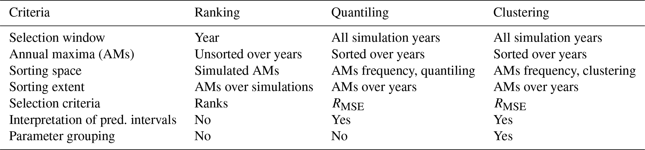
Table 1 Comparison of three methods for selecting representative parameter sets based on annual maxima (AMs).

2.3 Estimation of the predictive intervals for rare-flood simulations

While the three methods described in Sect. 2.2 vary in the way the representative parameter sets are selected (see Sect. 2.4 for a summary), each of these selection methods results in three (different) representative hydrological-simulation ensemble members and can be thought of as representing the lower (infimum), upper (median) and middle (supremum) interval of the full simulation range. The hydrological-model parameter sets corresponding to these are then noted as θ_inf, θ_med and θ_sup. The simulations corresponding to these three parameter sets together create the so-called predictive interval, which can be used for rare-flood simulation studies. Here, these predictive intervals constructed based on representative parameter sets correspond to 90 % predictive intervals (PIs).

2.4 Comparison of three selection methods

The major difference between these three methods is that the ranking method is evaluated based on individual simulation years using simple ranking of flow maxima independently of their frequency; i.e. it works on unsorted annual maxima. Note that in this way, for each y simulation year, a different rank order of the I hydrological-model parameter sets may be achieved. In an extreme case, where for each year different parameter sets are chosen, a choice of the representative sets over all simulation years may become problematic due to difficulties in identifying the parameter sets most frequently selected over all simulation years. The derived predictive intervals thus are sensitive to individual years of simulations, and their interpretation may be difficult (as they do not result from any flow frequency analysis).

In contrast to the ranking method, both other methods, i.e. quantiling and clustering, are performed on sorted AMs over all simulation years, i.e. in the flow frequency space. This enables statistical statements to be made about the selected parameter sets and about the predictive intervals constructed with the help of these parameter sets (as they are constructed on the entire simulation ensemble). Furthermore, selected parameter sets can be assumed to be representative over the entire simulation period (see Table 1 for a detailed overview of three methods). Finally, the clustering method splits all ensemble members (hydrological simulations) into three clusters, and so each parameter set can be attributed to corresponding clusters. This could be useful if one would like to extract more information on each cluster behaviour.

2.5 Assessment of the behaviour of the approach

Testing the methods for a time period different than the one that was used for the parameter ensemble downsizing is crucial for assessing how well the reduced ensembles substitute the whole simulation ensemble for the selection of representative parameter sets. Thus, we propose to assess the behaviour of the developed approach by repeating the selection of the three representative parameter sets with the three proposed methods with multiple (M) meteorological scenarios. Using multiple meteorological scenarios first enables us to account for the natural variability in the hydrological response due to climate variability and, second, gives us the possibility to evaluate the bias of the approach. Particularly, with the help of multiple meteorological scenarios we explore how the choice of the representative parameter sets θ_inf, θ_med and θ_sup depends on the meteorological scenario.

2.5.1 Leave-one-out cross-validation

To evaluate the three selection methods, we perform a leave-one-out cross-validation simulation study, in which a meteorological scenario S_r is removed from the analysis, and the selection of the representative parameter sets is executed based on all other remaining meteorological scenarios, i.e. using all m=1, 2, … M and m≠r. The evaluation of selection methods is then executed against the one meteorological scenario initially removed from the set. In detail, the following steps are executed for each of the three methods independently:

• a.

  Pick up and remove one meteorological scenario S_r from ${\mathit{S}}_{\mathrm{1},\mathrm{2},\mathrm{\dots }\mathrm{M}}$ scenarios available.

• b.

  Analyse all other meteorological scenarios $\mathit{\left\{}{\mathit{S}}_{\mathrm{M}-\mathrm{r}}\mathit{\right\}}=\mathit{\left\{}{\mathit{S}}_{\mathrm{1},\mathrm{2},\mathrm{\dots }\mathrm{M}}\mathit{\right\}}\setminus \mathit{\left\{}{\mathit{S}}_{\mathrm{r}}\mathit{\right\}}$, each containing I ensemble members resulting from I hydrological-model parameter sets, $\mathit{\left\{}H\right({\mathit{\theta }}_i\left|{\mathit{S}}_{\mathrm{m}-\mathrm{r}}\right)\mathit{\}}$, for i=1,2, … I, m=1, 2, … M and m≠r and based on the selected three representative parameter sets ${\mathit{\theta }}_{\inf ,\mathrm{m}-\mathrm{r}}$, ${\mathit{\theta }}_{\mathrm{med},\mathrm{m}-\mathrm{r}}$ and ${\mathit{\theta }}_{\sup ,\mathrm{m}-\mathrm{r}}$ as described in Sect. 2.2.

• c.

  Estimate the predictive intervals of these S_M−r meteorological scenarios as the band spread between $H\left({\mathit{\theta }}_{\inf ,\mathrm{m}-\mathrm{r}}\right|{\mathit{S}}_{\mathrm{m}-\mathrm{r}})$ and $H\left({\mathit{\theta }}_{\sup ,\mathrm{m}-\mathrm{r}}\right|{\mathit{S}}_{\mathrm{m}-\mathrm{r}})$, the interval defined in step (b).

• d.

  Evaluate the meteorological scenario S_r removed at step (a) against the predictive intervals of S_M−r meteorological scenarios to assess how well the defined identified intervals represent the ensemble members of this S_r meteorological scenario (see Sect. 2.6 for assessment criteria).

The simulation is repeated M times to use each meteorological scenario once. In other words, this test evaluates how well the selection methods applied to all but one scenario can predict the full simulation range of the left-out scenario.

2.5.2 Multi-scenario evaluation

To further evaluate the three methods, we perform a simulation study using multiple (M) meteorological scenarios. In this study, the three selection methods are executed on one meteorological scenario randomly (without replacement) selected from the M available scenarios and evaluated against all remaining scenarios. In detail, the following steps are executed for each of the three methods independently:

• a.

  Pick up one meteorological scenario S_p out of the ${\mathit{S}}_{\mathrm{1},\mathrm{2},\mathrm{\dots }\mathrm{M}}$ scenarios available.

• b.

  Analyse the I simulated hydrological ensemble members of this scenario H(θ_i|S_p), i=1, 2, … I, resulting from I hydrological-model parameter sets θ_i for S_p, and select three representative parameter sets corresponding to θ_inf,p, θ_med,p and θ_sup,p, as described in Sect. 2.2.

• c.

  For all other remaining meteorological scenarios {${\mathit{S}}_{\mathrm{M}-\mathrm{p}}\mathit{\}}=\mathit{\{}{\mathit{S}}_{\mathrm{1},\mathrm{2},\mathrm{\dots }\mathrm{M}}\mathit{\}}\setminus \mathit{\{}{\mathit{S}}_{\mathrm{p}}\mathit{\}}$, take all hydrological ensemble members {H(θ_i|S_m)} for m=1, 2, … M and m≠p that correspond to θ_inf,p, θ_med,p and θ_sup,p. This results in M−1 model simulations for θ_inf,p, θ_med,p and θ_sup,p, one per meteorological scenario.

• d.

  Compute the 5th percentile for $\mathit{\left\{}H\right({\mathit{\theta }}_{\inf ,\mathrm{p}}\left|{\mathit{S}}_{\mathrm{m}}\right)\mathit{\}}$, the 50th for $\mathit{\left\{}H\right({\mathit{\theta }}_{\mathrm{med},\mathrm{p}}\left|{\mathit{S}}_{\mathrm{m}}\right)\mathit{\}}$ and the 95th for $\mathit{\left\{}H\right({\mathit{\theta }}_{\sup ,\mathrm{p}}\left|{\mathit{S}}_{\mathrm{m}}\right)\mathit{\}}$ for m=1, 2, … M and m≠p. The computed 5th and 95th percentiles together are assumed to describe the predictive intervals.

• e.

  Evaluate the predictive intervals against all S_M−p meteorological scenarios for assessing how well the identified prediction intervals represent the ensemble members of these S_M−p scenarios (see Sect. 2.6).

The steps (a)–(e) are repeated M times to use each meteorological scenario once. We call this evaluation a multi-scenario evaluation because the evaluation is performed using multiple meteorological scenarios at once (S_M−p) in contrast to the leave-one-out cross-validation (Sect. 2.5.1), where the evaluation is performed against only one meteorological scenario (S_r). This test quantifies how well the methods applied to a single scenario are transferable to all other scenarios.

2.6 Evaluation criteria

2.6.1 Visual assessment

The simplest way of assessing the behaviour of these three methods is a visual inspection of curves plotted in the frequency space (e.g. using Gumbel distribution for plotting), which can tell us how well the selected members reproduce the simulation ensemble and particularly whether the assignment of the representative parameter sets is correct or not. For this purpose, we propose to plot all simulated hydrological ensemble members together with the selected representative members in the frequency space for each considered meteorological scenario m individually and to visually assess the assignment of the three selected parameter sets, θ_inf,m, θ_med,m and θ_sup,m, and the corresponding intervals, i.e. $H\left({\mathit{\theta }}_{\inf ,\mathrm{m}}\right|{\mathit{S}}_{\mathrm{m}})$, $H\left({\mathit{\theta }}_{\mathrm{med},\mathrm{m}}\right|{\mathit{S}}_{\mathrm{m}})$ and $H\left({\mathit{\theta }}_{\sup ,\mathrm{m}}\right|{\mathit{S}}_{\mathrm{m}})$. The order of the intervals' assignment is assumed to be correct if it holds in the frequency space that

$$\begin{array}{}\text{(4)}& H\left({\mathit{\theta }}_{\inf ,\mathrm{m}}|{\mathit{S}}_{\mathrm{m}}\right)\le H\left({\mathit{\theta }}_{\mathrm{med},\mathrm{m}}|{\mathit{S}}_{\mathrm{m}}\right)\le H\left({\mathit{\theta }}_{\sup ,\mathrm{m}}|{\mathit{S}}_{\mathrm{m}}\right).\end{array}$$

We further define a ratio of incorrectly attributed scenarios with mixed-up intervals, i.e. for which Eq. (4) does not hold, as a measure of the bias as

$$\begin{array}{}\text{(5)}& R_{\mathrm{bias}}=\sum _{m=\mathrm{1}}^{\mathrm{M}}{\displaystyle \frac{R_{\mathrm{m}}}{M}},\end{array}$$

where R_m is computed for the mth scenario as

$$\begin{array}{}\text{(6)}& \begin{array}{rl}& R_{\mathrm{m}}=\\ & \left\{\begin{array}{cl}\mathrm{0}& \mathrm{if}H\left({\mathit{\theta }}_{\inf ,\mathrm{m}}|{\mathit{S}}_{\mathrm{m}}\right)<H\left({\mathit{\theta }}_{\mathrm{med},\mathrm{m}}|{\mathit{S}}_{\mathrm{m}}\right)<H\left({\mathit{\theta }}_{\sup ,\mathrm{m}}|{\mathit{S}}_{\mathrm{m}}\right)\\ \mathrm{1}& \mathrm{else}\end{array}\right..\end{array}\end{array}$$

2.6.2 Quantitative assessment

To quantitatively compare the three selection methods, we propose to compute the five following metrics:

• I.

  The ratio of simulation points in the frequency space, i.e. sorted annual maxima, lying outside the predictive intervals is computed for each mth scenario as

  $$\begin{array}{}\text{(7)}& R_{\mathrm{spo},\mathrm{m}}=\sum _{i=\mathrm{1}}^I\sum _{j=\mathrm{1}}^J{\displaystyle \frac{R_{\mathrm{spo},\mathrm{m},i,j}}{I\cdot J}},\end{array}$$

  where $R_{\mathrm{spo},\mathrm{m},i}$ is the ratio for each ith hydrological-model parameter set of the meteorological scenario m and is computed for each simulation point j (sorted annual maximum) as

  $$\begin{array}{}\text{(8)}& \begin{array}{rl}& R_{\mathrm{spo},\mathrm{m},i,j}=\\ & \left\{\begin{array}{cl}\mathrm{0}& \mathrm{if}{H}_j\left({\mathit{\theta }}_{\inf ,\mathrm{m}}|{\mathit{S}}_{\mathrm{m}}\right)\le H_j\left({\mathit{\theta }}_i|{\mathit{S}}_{\mathrm{m}}\right)\le H_j\left({\mathit{\theta }}_{\sup ,\mathrm{m}}|{\mathit{S}}_{\mathrm{m}}\right)\\ \mathrm{1}& \mathrm{else}\end{array}\right..\end{array}\end{array}$$
• II.

  In the leave-one-out cross-validation, the ratio of hydrological-simulation ensemble members lying outside the predictive intervals is computed for each mth scenario as

  $$\begin{array}{}\text{(9)}& R_{\mathrm{hso},\mathrm{m}}=\sum _{i=\mathrm{1}}^I{\displaystyle \frac{R_{\mathrm{hso},\mathrm{m},i}}{I}},\end{array}$$

  where $R_{\mathrm{hso},\mathrm{m},i}$ is the ratio computed for each ith ensemble member as

  $$\begin{array}{}\text{(10)}& \begin{array}{rl}& R_{\mathrm{hso},\mathrm{m},i}=\\ & \left\{\begin{array}{cl}\mathrm{0}& \mathrm{if}H\left({\mathit{\theta }}_{\inf ,\mathrm{m}}|{\mathit{S}}_{\mathrm{m}}\right)\le H\left({\mathit{\theta }}_i|{\mathit{S}}_{\mathrm{m}}\right)\le H\left({\mathit{\theta }}_{\sup ,\mathrm{m}}|{\mathit{S}}_{\mathrm{m}}\right)\\ \mathrm{1}& \mathrm{else}\end{array}\right..\end{array}\end{array}$$
• III.

  In the multi-scenario evaluation, the ratio of meteorological scenarios lying outside the predictive intervals is computed for each scenario p as

  $$\begin{array}{}\text{(11)}& R_{\mathrm{mso},\mathrm{p}}=\sum _m^M{\displaystyle \frac{R_{\mathrm{mso},\mathrm{m}}}{M-\mathrm{1}}}m=\mathrm{1},\mathrm{2},\mathrm{\dots }M\mathrm{and}m\ne p,\end{array}$$

  where R_mso,m is computed as

  $$\begin{array}{}\text{(12)}& \begin{array}{rl}& R_{\mathrm{mso},\mathrm{m}}=\\ & \left\{\begin{array}{cl}\mathrm{0}& \mathrm{if}H\left({\mathit{\theta }}_{\inf ,\mathrm{m}}|{\mathit{S}}_{\mathrm{m}}\right)\le H\left({\mathit{\theta }}_i|{\mathit{S}}_{\mathrm{m}}\right)\le H\left({\mathit{\theta }}_{\sup ,\mathrm{m}}|{\mathit{S}}_{\mathrm{m}}\right)\forall i=\mathrm{1},\mathrm{2},\mathrm{\dots }I\\ \mathrm{1}& \mathrm{else}\end{array}\right..\end{array}\end{array}$$
• IV.

  Relative band spread of PIs (R_ΔPIs) is computed for both tests and compares the spread of PIs constructed with the representative parameter sets versus 90 % PIs of the full hydrological ensemble. In detail, R_ΔPIs is computed for each mth scenario as

  $$\begin{array}{}\text{(13)}& \begin{array}{rl}{R}_{\mathrm{\Delta }\mathrm{PIs},\mathrm{m}}=& \sum _j^J{\displaystyle \frac{S_{\mathrm{PIs},\mathrm{repr}.,\mathrm{m}}}{S_{\mathrm{PIs},\mathrm{full},\mathrm{m}}}}m=\mathrm{1},\mathrm{2},\mathrm{\dots }M\\ & \mathrm{and}j=\mathrm{1},\mathrm{2},\mathrm{\dots }J,\end{array}\end{array}$$

  where $S_{\mathrm{PIs},\mathrm{repr}.,\mathrm{m}}$ and $S_{\mathrm{PIs},\mathrm{full},\mathrm{m}}$ are band spreads of the 90 % PIs constructed with the representative parameter sets and with the full hydrological ensemble. The band spread is computed as a difference between the upper (or supremum) and the lower (or infimum) interval at each jth simulation point in the frequency space.

• V.

  Overlapping pools of PIs (R_OPPIs) are computed for both tests in the frequency space by taking the Gumbel variate and discharge values of sorted AMs as coordinates of the PI pools. In detail, R_OPPIs of PIs constructed with the representative parameter sets is computed for each mth scenario as

  $$\begin{array}{}\text{(14)}& \begin{array}{rl}{R}_{\mathrm{OPPIs},\mathrm{m}}& =\sum _j^J{\displaystyle \frac{\left(k_j-k_{j-\mathrm{1}}\right)}{\mathrm{2}}}\left(H\left({\mathit{\theta }}_{\sup ,\mathrm{m},j}\right)\right.\\ & +H\left({\mathit{\theta }}_{\sup ,\mathrm{m},j-\mathrm{1}}\right)-H\left({\mathit{\theta }}_{\inf ,\mathrm{m},j}\right)\\ & \left.-H\left({\mathit{\theta }}_{\inf ,\mathrm{m},j-\mathrm{1}}\right)\right)m=\mathrm{1},\mathrm{2},\mathrm{\dots }M\\ & \mathrm{and}j=\mathrm{2},\mathrm{3},\mathrm{\dots }J.\end{array}\end{array}$$

  In a similar way, R_OPPIs is computed for the full hydrological ensemble using the pool restricted by the 90 % PIs, i.e. taking the 5 % and 95 % intervals as pool borders.

With respect to R_spo, the question arises of how to define the ratio of simulation points outside the predictive intervals if multiple hydrological simulations (leave-one-out cross-validation) or multiple meteorological scenarios (multi-scenario evaluation) are considered. Here we propose to use the 50th percentile to characterize the ratio of the majority of simulation points lying outside the computed predictive intervals for each of the methods.

In a similar way, for R_hso and R_mso an additional condition must be defined, i.e. how many out of J hydrological-simulation points for R_hso or how many out of I hydrological-simulation ensemble members for R_mso must lie outside the defined predictive intervals so that the hydrological simulation H(θ_i|S_m) or the meteorological scenario S_m is considered to be outside these intervals. For this purpose we define the rejection threshold r_thr (dimensionless) that has to be reached so that the meteorological scenario or hydrological simulation is assumed to be outside the predictive intervals. In this work, we consider the two following values for r_thr: {0.50, 0.10}.

With regards to R_ΔPIs, we propose to compute the relative band spread as a mean over all sorted AMs at first. Also, to focus more on rare floods, we propose to compute means of rare floods limited by different Gumbel variates. Here we computed R_ΔPIs for the upper half of AMs ($R_{\mathrm{\Delta }\mathrm{PIs},j\ge \mathrm{51}}$), for the uppermost 10 AMs ($R_{\mathrm{\Delta }\mathrm{PIs},j\ge \mathrm{91}}$) and the uppermost 5 AMs ($R_{\mathrm{\Delta }\mathrm{PIs},j\ge \mathrm{96}}$).

These five metrics are computed for all three methods and for all M meteorological scenarios, and the median values over these M scenarios are taken as a measure for comparing the three methods.

Figure 3 Location of the Dünnern at Olten catchment with a river network extracted from Swiss Map Vector 25 (SwissTopo, 2008).

3 Experimental set-up

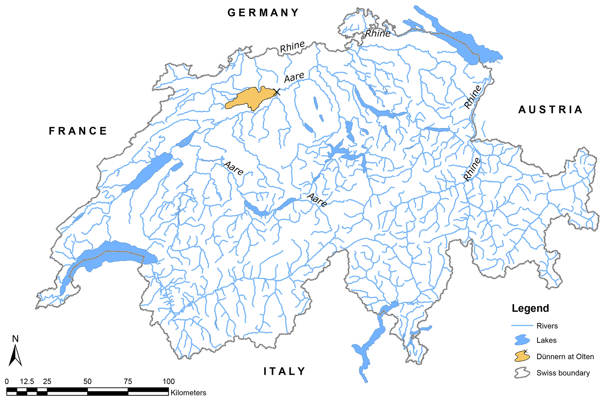
3.1 Study catchment

For testing the methods developed here, a small close-to-natural catchment is preferable, i.e. with only little anthropogenic influence, in which hydrological responses are transparent, and the generation of rare floods (peaks) is not affected by human constructions (dams, bridges). For this purpose, the Dünnern stream at Olten catchment with an area of 196 km² is selected, located in the Jura region in Switzerland (Fig. 3). The Dünnern stream is a tributary of the Aare river and belongs to the basin of the Rhine river. The mean elevation of the Dünnern at Olten catchment is 711 m a.s.l., with an elevation span from 400 to 760 m a.s.l. The flow regime is defined as nival pluvial jurassien (Weingartner and Aschwanden, 1992; Schürch et al., 2010), with high flows in winter and spring and low flows in autumn. With no direct human influence within the entire catchment known, it can be assumed to be close to natural (BAFU, 2017). This catchment is part of a large-scale extreme-flood modelling effort in Switzerland for the entire Aare catchment (Viviroli et al., 2020).

3.2 Hydrological model and calibration data

To simulate the hydrological catchment responses to meteorological scenarios, the HBV model (Hydrologiska Byråns Vattenbalansavdelning) is used. The HBV model is a semi-distributed bucket-type model, and it consists of four main routines: (1) precipitation excess, snow accumulation and snowmelt; (2) soil moisture; (3) groundwater and streamflow responses; and (4) run-off routing using a triangular weighting function. Due to the presence of the snow component, the HBV model is applicable to mountainous catchments (e.g. Jost et al., 2012; Addor et al., 2014; Breinl, 2016; Griessinger et al., 2016; Sikorska and Seibert, 2018b).

In this study, the version HBV light (Seibert, 1997; Seibert and Vis, 2012) with 15 calibrated parameters is used; see Table A1 for details on model parameters and their calibration ranges. Such a set-up of the HBV light was previously successfully applied in Swiss catchments (e.g. Sikorska and Seibert, 2018a; Brunner et al., 2018c; Brunner and Sikorska-Senoner, 2019; Müller-Thomy and Sikorska-Senoner, 2019; Westerberg et al., 2020). Model inputs are time series of precipitation and air temperature and long-term averages of seasonally varying estimates of potential evaporation, all being area-average values for the entire catchment. These inputs are next redistributed along predefined elevation bands using two different constant altitude-dependent correction factors for precipitation and temperature. The model output is streamflow at the catchment outlet at time steps identical to input data (hourly in this study).

For the study catchment, meteorological inputs (hourly precipitation totals, hourly air temperature means, average hourly evaporation sums) for the HBV model are derived from observed records from meteorological stations and are averaged to the mean catchment values using the Thiessen polygon method. The recorded continuous hourly streamflow data at the catchment outlet (Olten station) cover the period 1990–2014.

3.3 Identification of multiple HBV parameter sets

To derive multiple parameter sets of the HBV model, we propose a heuristic approach that relies on multiple independent model calibration trials using a genetic-algorithm (GA) approach (Appendix A). By using independent model runs, the possibility of being trapped in the same local optimum should be reduced. The genetic algorithm is used together with a multi-objective function F_obj with three scores: the Kling–Gupta efficiency (R_KGE), the efficiency for peak flows (R_PEAK) and a measure based on the mean absolute relative error (R_MARE). R_PEAK is defined in a similar way to the Nash–Sutcliffe efficiency but using peak flows instead of the entire time series. While both R_KGE and R_PEAK focus on high (peak) flows, R_MARE is sensitive to low flows. See Appendix B for equations.

F_obj is obtained through weighing these metrics as follows:

$$\begin{array}{}\text{(15)}& F_{\mathrm{obj}}=\mathrm{0.3}{R}_{\mathrm{KGE}}+\mathrm{0.5}{R}_{\mathrm{PEAK}}+\mathrm{0.2}{R}_{\mathrm{MARE}}.\end{array}$$

The weights in F_obj are chosen following our previous experience in modelling Swiss catchments (Sikorska et al., 2018; Westerberg et al., 2020). The available observational datasets are split into a calibration (1990–2005) and a validation (2006–2014) period. Evaluation of the model in the independent period is important as the model is applied to simulate time series outside the calibration period. To set up the initial conditions, 1 year of model simulations is discarded from the calibration simulation, and the remaining are used for model performance computation. For the validation period, the initial conditions are taken from the calibration simulation.

Here, the genetic algorithm is run 100 times, resulting in 100 independent optimal parameter sets (see Fig. C1). These 100 parameter sets represent similarly likely solutions to model hydrological responses in this catchment and can be explained by the equifinality of hydrological-model parameters (Beven and Freer, 2001). The median model efficiency measured with F_obj over all 100 runs is 0.7 in the calibration and in the validation periods, which can be assumed to be a good model performance on an hourly scale. Also, diagnostics of the Nash–Sutcliffe efficiency and the peak efficiency demonstrate that the model performs well in the range of high flows, which are mostly important for simulation of rare floods studied in this paper (see Fig. C2).

Note that the way to derive 100 parameter sets described above is one possible approach, and other calibration methods could be used (e.g. Monte Carlo or bootstrapping).

3.4 Generation of synthetic meteorological scenarios using a weather generator

Meteorological scenarios of synthetic precipitation and temperature data for the Dünnern at Olten catchment are generated with the weather generator model GWEX developed by Evin et al. (2018) and referred to in their paper as GWEX_Disag. This stochastic model is a multi-site precipitation and temperature model that reproduces the statistical behaviour of weather events on different temporal and spatial scales. The major property of GWEX is that it uses marginal heavy-tailed distributions for generating extreme-precipitation and extreme-temperature conditions. Moreover, it has been developed to generate long-term (≈1000 years) meteorological scenarios. GWEX_Disag generates precipitation amounts at a 3 d scale and then disaggregates them to a daily scale using a method of fragments (for details on the precipitation model, see the work of Evin et al., 2018, and for details on the temperature model, see the work of Evin et al., 2019).

The meteorological scenarios used in this study are a subset from the long-term meteorological scenarios developed for the entire Aare river basin using recorded data from 105 precipitation stations and from 26 temperature stations in Switzerland (Evin et al., 2018, 2019). For this larger-scale research project, GWEX_Disag was set up using daily precipitation and temperature data from the period 1930–2015 and hourly records of precipitation and temperature from 1990–2015 for the Aare river basin. The daily values generated with GWEX_Disag were then disaggregated to hourly values using the meteorological analogues method, which for each day in the simulated dataset finds an analogue day in observed data, i.e. with a known hourly time structure. Next, catchment means were computed using the Thiessen polygon method (using three stations located close by).

For the present study, 100 different meteorological scenarios (precipitation and temperature) covering the same time frame of 100 years at an hourly time step are available for the Dünnern at Olten catchment (see Fig. D1 for an overview of meteorological scenarios). The simulated data are assumed to be representative of current climate conditions, i.e. neither variation due to climate or land use change nor river modification is considered. Thus, differences between scenarios are exclusively due to the natural variability in the meteorological time series and modelled by the GWEX_Disag weather generator.

3.5 Generation of synthetic hydrological-simulation ensembles

Finally, for our analysis, 100 meteorological scenarios with continuous data of 100 years of precipitation and temperature and 100 calibrated parameter sets of the HBV model are available. This number of 100 was chosen as a compromise between minimizing the intensive model calibrations and the simulations at an hourly time step and maximizing the information content of the hydrological-parameter sample and the climate variability. We have chosen the same number of 100 for meteorological scenarios, parameter sets and simulation years to not favour any of these components in the methods' comparison. These 100 meteorological scenarios are used as input into the HBV model to generate streamflow time series with 100 different HBV parameter sets. To set up the initial conditions of the model, a 1-year warming-up period is always used prior to the simulation period. To get an overview of the variability in such hydrological ensembles, see Fig. D2.

From each of these continuous hydrological simulations, 100 annual maxima (AMs; one per calendar year) are selected (see Fig. 4). This results in the following analysis set-up:

• I=100 and i=1, 2, … 100;

• J=100, y=1, 2, … 100 and j=1, 2, … 100;

• M=100 and m=1, 2, … 100,

with $\mathrm{100}\times \mathrm{100}\times \mathrm{100}$ combinations of the annual maximum × hydrological-model parameter set × meteorological scenario.

Figure 4 Set-up of the experimental study.

These series of AMs are next used to test the developed methods of selecting the representative parameter sets from the ensemble of 100 available sets.

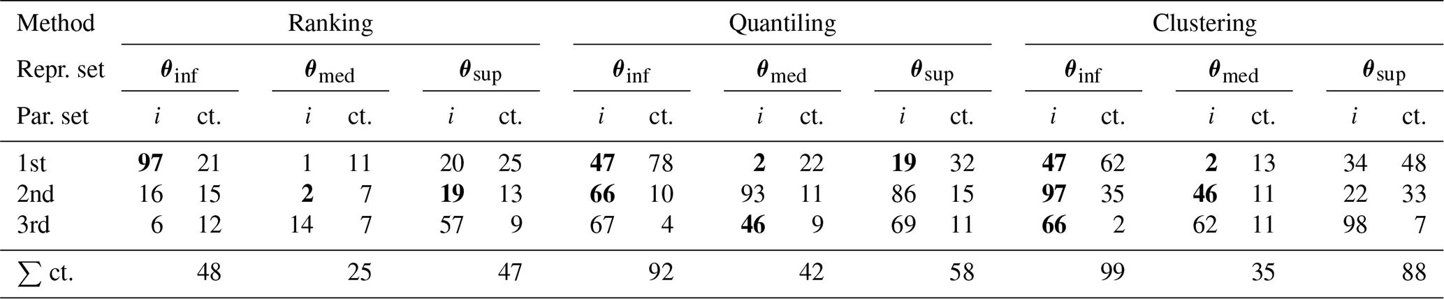
Table 2 The three representative parameter sets θ_inf, θ_med and θ_sup most frequently selected with three methods. The i stands for the set index and ct. for the number of counts. The expression ∑ ct. stands for the sum of counts for the first three most frequently selected sets. Bold font indicates parameter set indices which are selected as representative with at least two methods among the three sets most frequently chosen.

4 Results

4.1 Representative parameter sets

The representative parameter sets selected with each of the three methods are summarized over all 100 meteorological scenarios in Table 2, which presents the three most frequently chosen hydrological parameter sets for each method.

Although different parameter sets are usually selected by different methods, in a few cases the same set is chosen with more than one selection method. Among the first three most frequently chosen sets, the same parameter set is selected as the median set once for all three methods and several times for at least two methods.

The variability in the selected hydrological parameter sets is presented in Fig. 5. As can be seen from the figure, some parameters presented smaller and others larger variability in selected sets. It also appears that different values are selected for the infimum, median and supremum set but not always. Among the three selection methods, the ranking method (marked in green) has the largest spread of parameter values for most of the parameters. The clustering (blue) and quantiling (yellow) selection methods seem to choose more extreme parameter values for both, i.e. infimum and supremum sets. Looking at different model routines no clear patterns could be seen regarding the choice of parameter sets. It appears however that the representative parameters from the response (blue) and soil moisture (yellow) routines have a smaller spread than those from the snow routine (grey) as they are more often outside and further away from the interquartile ranges (grey boxplots).

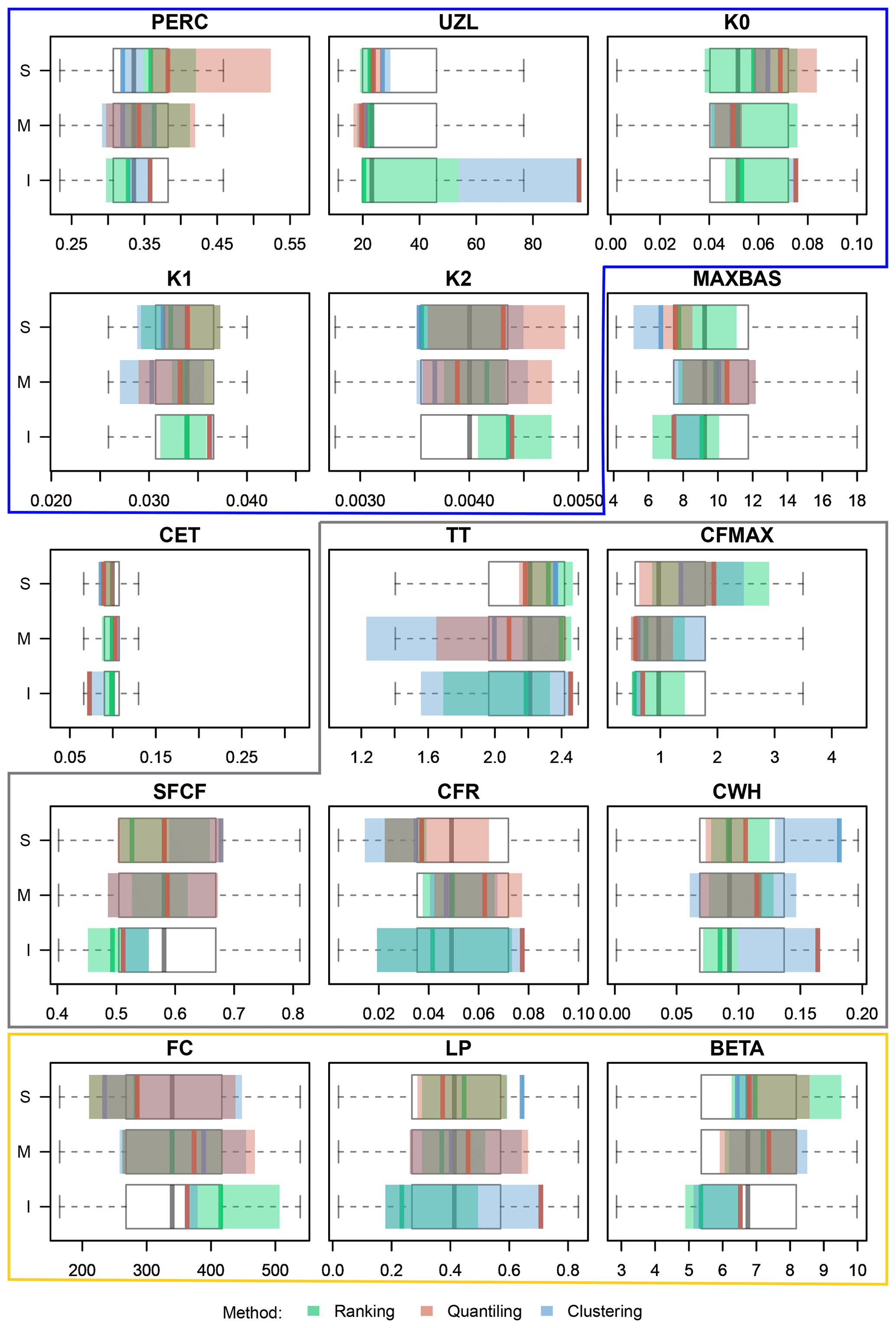
Figure 5 Box plots showing the variability in the hydrological parameter sets selected as the representative parameter sets over 100 meteorological scenarios chosen with three methods. The white box plots illustrate the entire parameter ensemble (i.e. 100 sets); outliers are not presented. I: infimum; M: median; and S: supremum set. Units as in Table A1. The blue box surrounds parameters from the response routine, the grey box from the snow routine and the yellow from the soil moisture routine. MAXBAS is the only parameter from the routing routine, and CET is a potential-evaporation correction factor.

4.2 Infimum, median and supremum intervals

Using the selected representative sets, representative intervals for rare-flood estimations are constructed for each of the 100 meteorological scenarios and each of the three selection methods. Examples of these intervals for two meteorological scenarios are presented in Figs. 6 and 7. Note that apart from selecting representative intervals, the clustering method leads to grouping all ensemble members into three selected clusters.

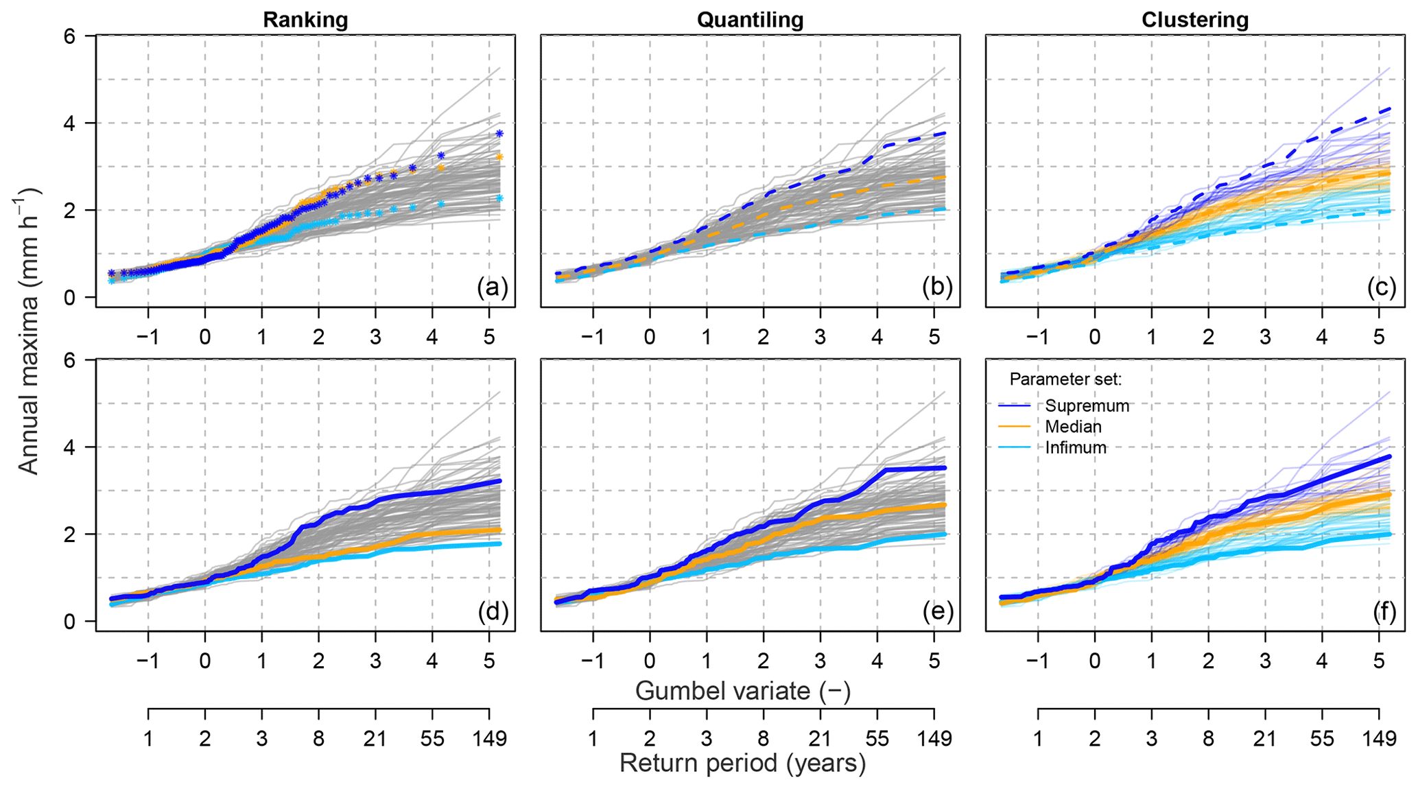
Figure 6 Example of the representative parameter sets' selection with three methods in the Dünnern at Olten catchment (meteorological scenario m=14). The top panel presents intermediate steps of selecting the representative sets and the bottom panel the finally constructed intervals, i.e. infimum, median and supremum. The dashed lines (top panel) indicate the computed representative intervals (i.e. steps a–c in ranking and clustering and a–b in quantiling), and the solid lines (bottom panel) indicate the hydrological-simulation members corresponding to the parameter sets selected as representative (step d in ranking and quantiling and e in clustering).

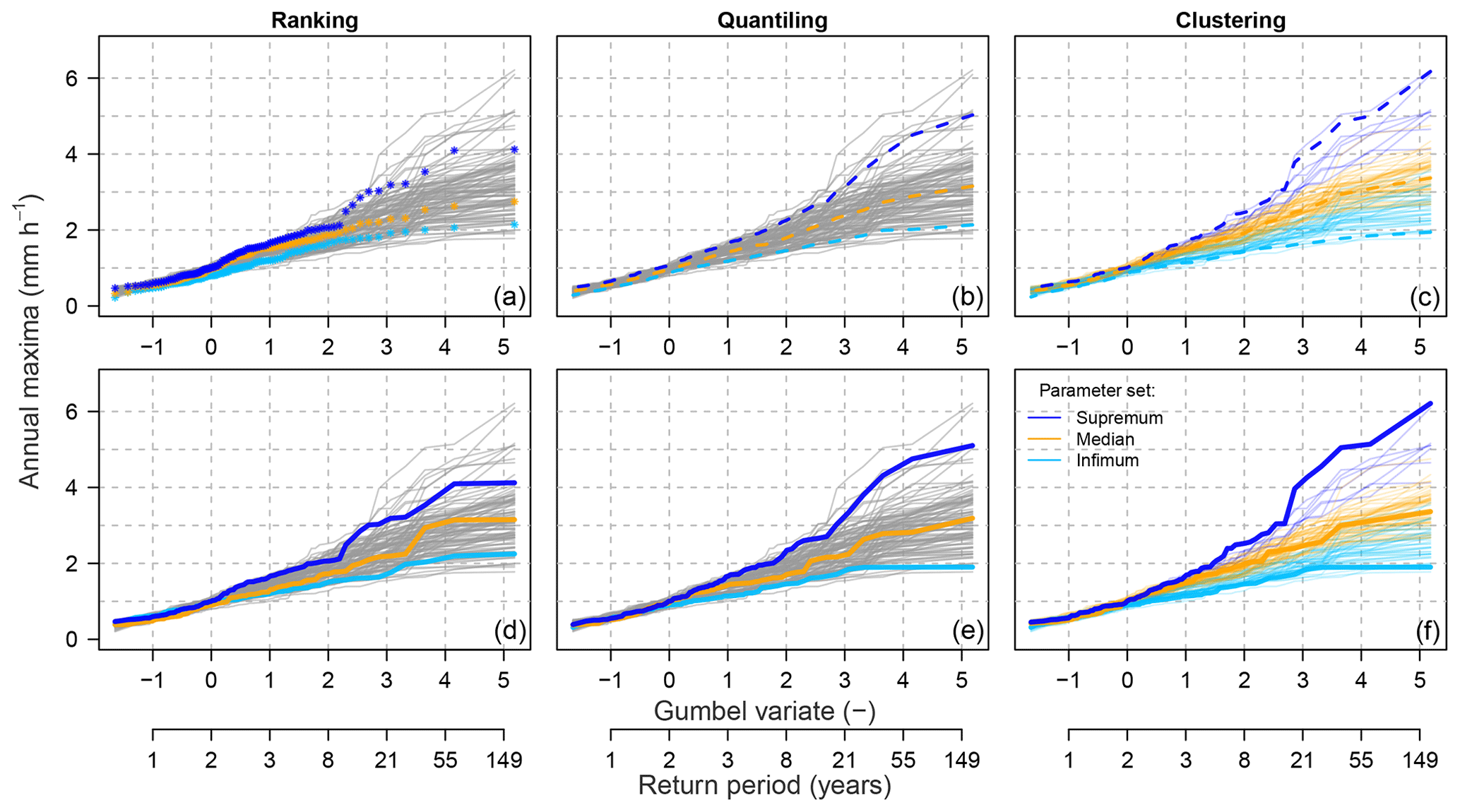
Figure 7 Example of the representative parameter sets' selection with three methods in the Dünnern at Olten catchment (meteorological scenario m=93); description as in Fig. 6.

According to a first visual assessment, these three methods lead to slightly different constructed frequency intervals particularly in the upper tail of the distribution, i.e. for the most rare (highest) flows, which are of highest interest. Moreover, the ranking method leads to less symmetrically spread intervals, with the median and infimum intervals lying close to each other. The other two methods lead to more symmetrically spread intervals.

For the quantitative assessment, the ratio of scenarios incorrectly attributed, i.e. with intervals being mixed up (R_bias), varies between the three methods and is the highest for the ranking method (R_bias=0.54). For the clustering method, the three intervals are always correctly ordered for all 100 meteorological scenarios tested (R_bias=0.0). For the quantiling method, this ratio is equal to R_bias=0.02 and thus is also very low. Hence, we can conclude that both clustering and quantiling methods provide correctly attributed intervals with a bias ≤2 %. For the ranking method, the correctness of the interval attribution is poor, and in more than 50 % of the meteorological scenarios, the simulations corresponding to the selected parameter sets lead to mixed-up frequency intervals.

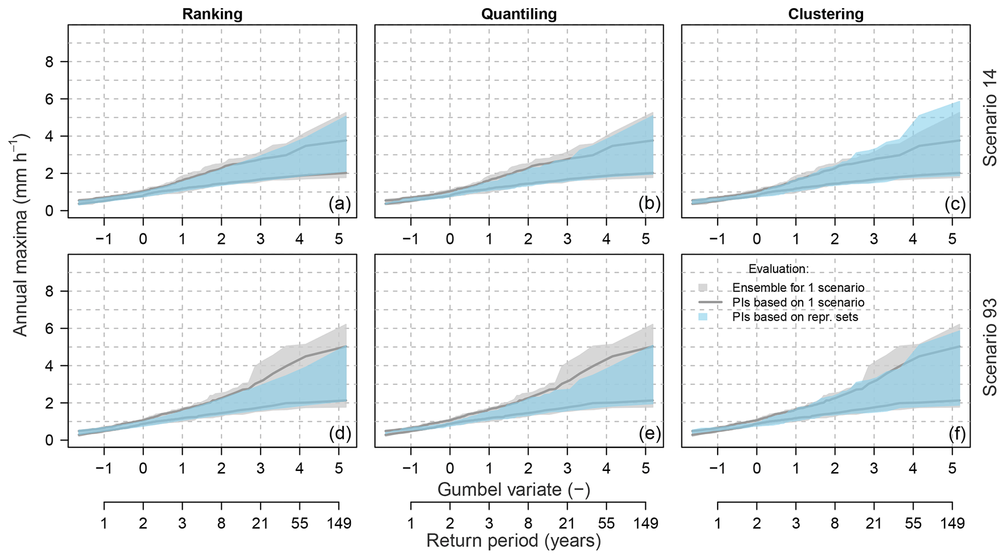
Figure 8 Example of leave-one-out cross-validation for the three selection methods and two meteorological scenarios. PIs represent the 90 % predictive intervals.

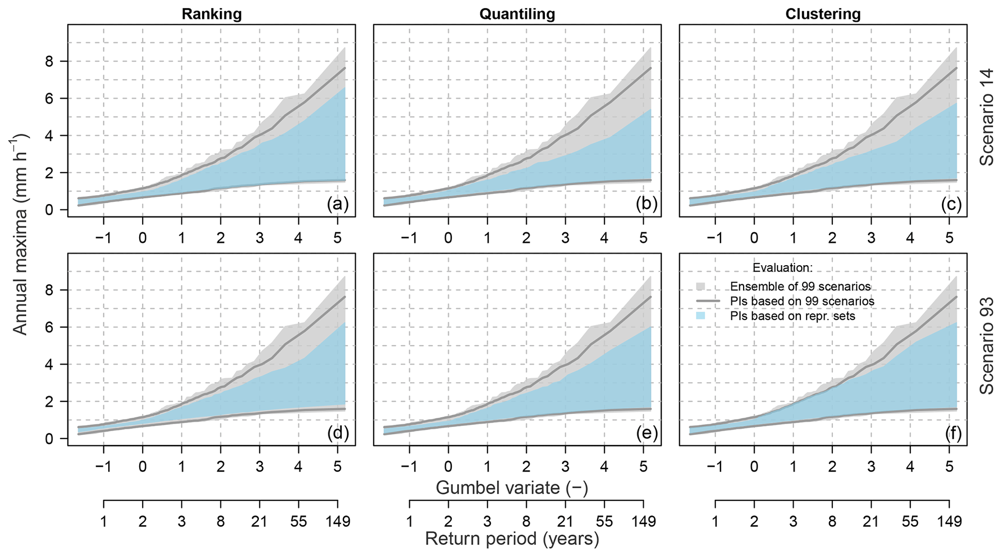
Figure 9 Example of multi-scenario evaluation for the three selection methods and two meteorological scenarios. PIs represent the 90 % predictive intervals.

4.3 Evaluation of the three selection methods

The behaviour of the three selection methods is further evaluated with the 100 meteorological scenarios using the leave-one-out cross-validation test (Sect. 2.5.1) and the multi-scenario evaluation method (Sect. 2.5.2) and corresponding metrics (Sect. 2.6.2). Examples for two meteorological scenarios are presented in Fig. 8 for the leave-one-out cross-validation test and in Fig. 9 for the multi-scenario evaluation. From the visual assessment, it is difficult to judge the methods as they seem to perform similarly well. However, the range of the predictive intervals obtained with 99 meteorological scenarios (one left out) is considerably narrower for ranking and quantiling on one hand and much wider for clustering on the other hand (Fig. 8). Accordingly, the correspondence between the prediction interval and the full simulation range of the left-out scenario differs between the methods (Fig. 9).

Table 3 Metrics of the behaviour of the approach for three methods of selecting representative parameter sets and the predictive intervals in the leave-one-out cross-validation and in the multiple-scenario evaluation. The values represent the median values over all 100 scenario runs.

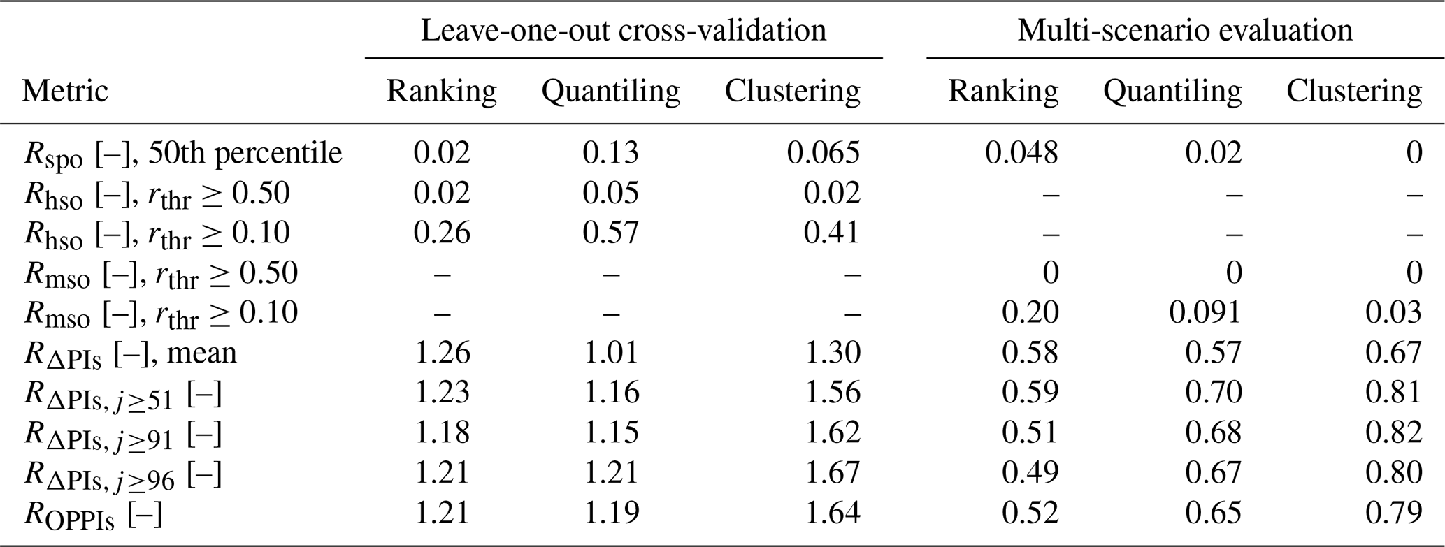
This is reflected in the quantitative assessment of the methods' behaviour, summarized in Table 3. Namely, the leave-one-out cross-validation reveals that the quantiling method receives the highest values for both evaluation criteria, i.e. the ratio of simulation points lying outside the predictive intervals (R_spo) and the ratio of hydrological-simulation ensemble members lying outside the predictive intervals (R_hso), both presented as median values over all scenarios. Thus, this method performed the poorest among all three methods tested here. Yet, with R_spo≤0.14 for the 50th percentile and R_hso≤0.05 for the threshold r_thr≥0.50, even this method can be qualified as behaving well based on the leave-one-out cross-validation. For the ranking and the clustering methods, similar values for these two metrics are achieved, with slightly lower values for the ranking method.

In summary, it can be said that all criteria values are relatively low for all three methods, and thus the computed criteria values can only be used to order the methods by their behaviour, while none of the methods are rejected.

In contrast to the above findings, the multi-scenario evaluation reveals different results, with R_spo being the lowest for clustering and the largest for the ranking method. Similarly, the ratio of meteorological scenarios lying outside the predictive intervals (R_mso) is the lowest for clustering and the highest for the ranking method (r_thr in Table 3).

Also, here all computed criteria values are relatively low, with R_spo≤0.05 for the 50th percentile and R_mso=0 for the threshold r_thr≥0.50 for the poorest-behaving method (ranking). Hence, again here all three methods can be qualified as behaving well based on the multi-scenario evaluation.

Analysis of overlapping PI pools (R_OPPIs) and relative band spreads (R_ΔPIs) shows that in the cross-validation test all methods provide bands that are wider than the 90% PIs computed using the full simulation ensemble. This should not be surprising as the selection of relative parameter sets is based on a larger sample of hydrological-model realizations (i.e. 99 scenarios) than the full ensemble for model assessment (i.e. single scenario). However, these metrics show large differences in the multi-scenario test, in which the clustering method outperforms the other two selection methods, particularly when the focus lies on rare floods (compare $R_{\mathrm{\Delta }\mathrm{PIs},j\ge \mathrm{51}}$, $R_{\mathrm{\Delta }\mathrm{PIs},j\ge \mathrm{91}}$ and $R_{\mathrm{\Delta }\mathrm{PIs},j\ge \mathrm{96}}$ in Table 3). The quantiling was the second-best method, while the ranking performed the worst. These observations are also confirmed when looking at the variability in these two metrics for different return periods (Fig. 10). A better performance of the clustering method can be again noticed in the range of rare floods. While quantiling performed worse than clustering, it was still better than the ranking method.

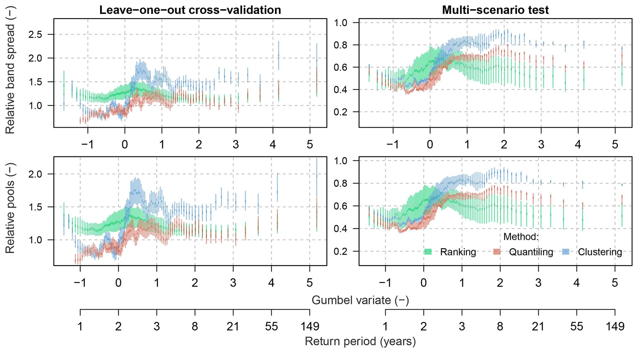
Figure 10 Evaluation of the leave-one-out cross-validation and the multi-scenario test for the three selection methods using the relative band spread (R_ΔPIs) and the relative overlapping pools (R_OPPIs), both computed with reference to the 90 % PIs of the full hydrological-simulation ensemble.

As it appears from the above, the rejection or acceptance of one of the three methods tested here is not straightforward. Apart from the ranking method, which was linked to a huge bias, both other methods, i.e. quantiling and clustering, performed similarly well. Yet, these methods provide quite different intervals (of a different spread). The validity and usefulness of these methods for selecting the representative parameter sets are thus further discussed below in Sect. 5.1. The detailed analysis of the relative band spread and the overlapping pools indicated however that the clustering method performed the best, particularly in the range of rare floods. The quantiling method was scored as the second best, while the ranking method performed poorest.

5 Discussion

5.1 Behaviour of three selection methods

The results from our experimental study demonstrate that generally all three methods are capable of selecting representative parameter sets that yield reliable predictive intervals in the frequency domain, i.e. all three methods are fit for purpose for extreme-flood simulation, with the ranking method performing, however, clearly less well than the others (larger bias, as visible in Sect. 4.2). As the developed methods rely on selecting three representative sets as infimum, median and supremum, they respect the maximum variability between individual ensemble members for a given meteorological scenario.

Table 4 Synthesis of scoring ranks attributed to the three methods for selecting representative parameter sets (based on quantitative metrics). The ranks are attributed descending from the best (1) to the worst (3) behaviour. The median scoring rank (last line) corresponds to the median over all criteria.

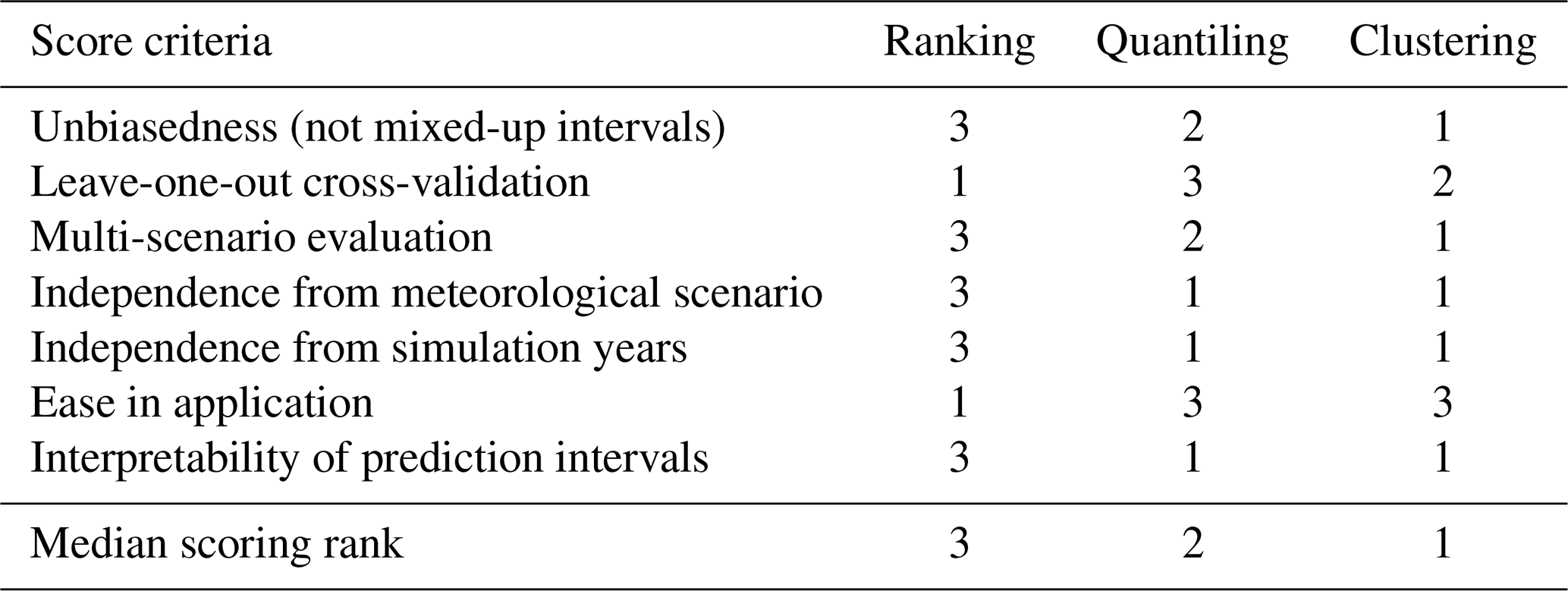
In the validation tests, the behaviour scores of the three methods, however, were attributed differently depending on the evaluation criteria. To further compare the methods, we provide a detailed discussion of the major differences below and present a synthesis of how the methods rank on average (averaged across all scenarios) for the quantitative evaluation criteria, which we support with further qualitative evaluation criteria (Table 4).

From the visual assessment, i.e. based on the method bias (R_bias), it clearly appears that the ranking method is the most biased method (with more than half of all meteorological scenarios having mixed-up intervals), while the other two methods can be considered to be unbiased with correctly attributed intervals for 98 % (quantiling) or more (clustering) of all meteorological scenarios considered here (Sect. 4.2, unbiasedness in Table 4). As expected, these findings are further confirmed by the results from the multi-scenario evaluation that yield the best behaviour for the clustering method and the worst for the ranking method (Sect. 4.3), particularly if the focus lies on rare floods as assessed by the relative band spread and the overlapping pools.

Interestingly, the leave-one-out cross-validation study, in contrast to the multi-scenario evaluation, attributes the lowest criteria value to the ranking method, i.e. ranks it as the best method (Table 4). This requires a careful interpretation and understanding of how the predictive intervals are constructed in both evaluation studies. In the leave-one-out cross-validation study, the representative parameter sets are selected, and the predictive intervals are constructed based on 99 meteorological scenarios and then evaluated against the full simulation range corresponding to the left-out scenario. In the multi-scenario evaluation, the representative parameter sets are selected based on a single scenario, and the predictive intervals are then assessed by applying these three selected sets (selected based upon a single scenario) to the other 99 meteorological scenarios. Hence, by comparing findings from these two evaluation studies, it appears that the ranking method performs poorly if using a single scenario for selecting the representative sets (multi-scenario evaluation). In exchange, the ranking method outperforms the two other methods when a high number of meteorological scenarios are used for selecting the representative parameter sets (leave-one-out cross-validation). This means that the ranking method strongly depends on the meteorological scenario choice, while the other two methods result in representative parameter sets that are transferable to other meteorological scenarios. We hence introduce here a criterion independence from meteorological scenario, which defines how strongly the selected sets depend on the meteorological scenario used for selection of representative parameter sets.

In a similar way, independence from simulation years will define how strongly the selected sets depend on the simulation years used for selection of the representative parameter sets. To make statements on that, one needs to recall how the selection methods are constructed: the ranking method, in fact, depends strongly on the selected simulation period (and hence on the meteorological scenario) because the selection of the representative parameter sets is performed on unsorted annual maxima for each simulated year independently. The other two methods are performed over the entire simulation period, which makes them less strongly dependent on individual simulation years. Nevertheless, the ranking method can be considered to be the (computationally and methodologically) easiest in application due to its selection criteria relying purely on ranking within individual simulation years. We call this criterion an ease in application. The other two methods need to be performed in the frequency space on sorted annual maxima over the entire simulation period and, in the case of the clustering method, require some additional computational effort (which remains low, however, compared to the hydrological simulation). The use of the frequency space in selecting the representative parameter sets helps, however, to interpret the constructed prediction intervals and to directly assign return periods to them. This speaks for their higher interpretability of prediction intervals as compared to the ranking method, in which interpretation of intervals is very limited (as they are selected without any flow frequency analysis).

Overall based on scoring results from Table 4, it appears that the clustering method behaves the best (with a median scoring rank of 1) due to its unbiasedness and due to a good performance achieved for all evaluation criteria, for both the leave-one-out cross-validation and the multi-scenario evaluation. Finally, this method was proven to perform the best if the focus lies on rare-flood simulations.

5.2 Limitations and perspectives

We should emphasize that the presented methods are independent of the selected hydrological-model calibration approach or from the selected hydrological-response model and are thus readily transferable to any similar simulation setting. Despite the fact that the calibration of a hydrological model lies beyond the scope of this paper, it is assumed that (at least) 100 parameter sets of a hydrological model can be made available for selecting the representative parameter sets. For that purpose, a hydrological model should be calibrated with observed data of a long enough record that covers rare floods so that rare floods could be realistically simulated. In this work, to derive 100 parameter sets, we proposed a heuristic approach that relies on multiple independent model calibration trials using a genetic-algorithm approach and a multi-objective function. This method represents an interesting solution to systematic sampling of the posterior parameter distributions (e.g. via Markov chain Monte Carlo sampling) or to any Monte Carlo method relying on a very high number of model runs. Its strength is that it can be applied for selecting parameter sets from independent model calibration settings (with different scores, calibration periods, etc.).

Note however that for the purpose of deriving 100 parameter sets, a continuous hydrological model does not necessarily require continuous calibration data, and it could be also calibrated to discrete data (e.g. using hydrological signatures; Kavetski et al., 2018). If no observed data or only too short records are available, model parameters can be acquired through regionalization approaches (see the work of Brunner et al., 2018a, for an overview of regionalization methods). The developed methods are of use for applications when a hydrological model should be employed for simulations of rare floods. If the use of a hydrological model is not possible, i.e. neither information for calibration nor sufficient information for parameter regionalization is available, these methods cannot be applied. Moreover, although the methods are tested with a bucket-type hydrological model, the most valuable application of the proposed methods would be to computationally more demanding hydrological models that can profit even more from a reduced computational demand.

Furthermore, the proposed approach is tested here using synthetic hydrological data, i.e. using streamflow simulations of the hydrological model in response to meteorological scenarios. We chose to use synthetic instead of real observed data to work with long enough continuous simulations that cover rare events and to minimize the focus of the model error arising from the calibration data and procedure. By using synthetic data as a reference (instead of observed data), the latter error can be neglected here. The proposed methods should be tested with more catchments and other models to verify the scoring of methods that was achieved in this study.

Selection methods proposed in this study enable one to choose representative parameter sets of a hydrological model and based on those to construct uncertainty predictive intervals (PIs) for extreme-flood analysis in the frequency space. Here, we tested the methodology using 100 meteorological scenarios that should represent the natural climate variability and in this way should provide independent conditions for methods' evaluation. Such a method for constructing PIs from a hydrological model ensemble is a powerful tool that opens several avenues for further detailed uncertainty analysis. For instance, one may be interested in contributions of different uncertainty sources into the total PIs constructed, e.g. coming from the hydrological model or the natural climate variability. As these two components are not linearly additive, their separation is not straightforward.

In addition, any ensemble simulation also encompasses other uncertainty sources of the modelling chain, such as those resulting from the weather generator, from the structure of the selected hydrological model, from the prediction of very rare flood events, etc. (Lamb and Kay, 2004; Schumann et al., 2010; Kundzewicz et al., 2017). To assess individual contributions of interest, a simple sensitivity analysis based on the variance variability could be recommended here, in which one uncertainty source is propagated through the method at once while other sources are kept at their mode or median values and in which the resulting PI spread is compared.

Downsizing the hydrological-model parameter sample can only aim to understand and characterize the hydrological part of the full hydrological ensemble resulting from a combination of multiple parameter sets and multiple meteorological scenarios. The variability in hydrological-model parameters arises from the parameter equifinality (Beven and Freer, 2001), and it can be overcome by using several hydrological-model parameter sets that should encompass the parametric and (implicitly) also other uncertainty sources. Our selection methods thus enable one to choose representative parameter sets from the hydrological-response point of view and in this way to cover the variability in hydrological responses with a reduced number of hydrological-model runs needed. These methods are however not applicable for characterizing the climate variability (nor for downsizing the number of meteorological scenarios needed).

Moreover, in developing the selection methods, we did not distinguish between different flood types such as heavy rainfall excess or intensive snowmelt events (Merz and Blöschl, 2003; Sikorska et al., 2015). Also, as we focused only on large annual floods (annual maxima), we did not represent the flood seasonality in our analysis. Yet, some recent works emphasize the need to include such information on the flood type (Brunner et al., 2017) or on flood seasonality (Brunner et al., 2018c) into bivariate analysis of floods or to represent a mixture of both flood type and flood seasonality in flood frequency analysis (Fischer et al., 2016; Fischer, 2018). Thus, the proposed selection methods could potentially be extended to account for different flood types during representative parameter selection, e.g. using automatic methods of flood type attribution from long discharge series (Sikorska-Senoner and Seibert, 2020). For that purpose, peak-over-threshold (POT) selection criteria of flood peaks could be more appropriate instead of a block selection (annual maximum) used here in constructing the simulated distributions of hydrological responses in order to cover a range of different flood processes.

Finally, we downsize the hydrological-model parameter sample to three sets which represent the predictive intervals of the full ensemble of hydrological responses fairly well given different meteorological scenarios. This number of three sets is motivated by the fact that it can be readily processed within a fully continuous ensemble-based framework using numerous climate settings. This is common practice in flood frequency analysis, and the three sets emulate the common practice of communicating median values along with prediction limits (Cameron et al., 2000; Blazkova and Beven, 2002; Lamb and Kay, 2004; Grimaldi et al., 2012b). For safety studies, these representative intervals should be additionally statistically proved.

Optionally, one could further downsize the hydrological-model parameter sample to two sets (i.e. infimum and supremum), which would represent the intervals only. Downsizing to more than three parameter sets (e.g. five or more) could have the advantage of containing more information on uncertainty intervals, e.g. in the case that they are asymmetric, and should be explored in further studies.

Possible applications of these selection methods include all studies where computational requirements are an issue, e.g. rare-flood analysis in safety studies concerning dams or bridge breaks; climate scenarios of these; and evaluation of rare floods due to changes in climatic variables using several emission scenarios and different uncertainty source propagation. Finally, these methods could be used for quantifying different uncertainty source contributions in rare-flood estimates but with less effort from the hydrological model as due to parametric uncertainty propagation.

6 Conclusions

In this study, we propose and test three methods for selecting the representative parameter sets of a hydrological model to be used within fully continuous ensemble-based simulation frameworks. The three selection methods are based on ranking, quantiling and clustering of simulation of annual maxima within a limited time window (100 years) that is much shorter than the full simulation period of thousands of years underlying the simulation framework. Based on a synthetic case study, we demonstrate that these methods are reliable for downsizing a hydrological-model parameter sample composed of 100 parameter sets to three representative sets that represent most of the full simulation range in the frequency space. Among the tested methods, the clustering method that selects parameter sets based on cluster analysis in the frequency space appears to outperform the others due to its unbiasedness, its transferability between meteorological scenarios and a better performance for rare floods. The ranking method, which is the only tested method that completes the parameter selection on non-sorted annual maxima, can clearly not be recommended for typical settings since it (i) tends to result in mixed-up prediction intervals in the frequency space and (ii) depends too strongly on the simulation period used for parameter selection and thus lacks transferability to other periods or other meteorological scenarios. Possible applications of these methods include all fully continuous simulation schemes for rare-flood analysis and particularly those for which computational constraints arise, such as safety studies or scenario analysis.

Appendix A: Details on the HBV model parameters and model calibration

For searching the best hydrological-model parameter sets within the defined parameter ranges (Table A1), a genetic-algorithm and Powell optimization (GAP) approach (Seibert, 2000) is used. This approach is executed in two major steps. Firstly, the GA optimization is performed and relies on an evolutionary mechanism of selection and recombination of a user-defined number of parameter sets (i.e. parameter population) randomly selected within the defined parameter ranges. The principle idea of this searching relies on regenerating the parameter sets from the subgroup of parameter sets selected using the defined objective function F_obj as a criterion to choose the parameters that give the highest value of F_obj at the previous step of the model calibration. The search for the best parameter set is terminated at a user-defined maximum number of model interactions and results in a selected optimal parameter set. Secondly, the optimal parameter set obtained at the previous step is used as a starting point for a local optimization search using Powell's quadratically convergent method (Press et al., 2002). The parameter set finally achieved from the local optimization is retained as the best set. In this study, the total number of model interactions is set to 2500 for the GA and 500 for the local Powell's optimization.

Table A1 Parameter ranges for the calibration of the HBV model.

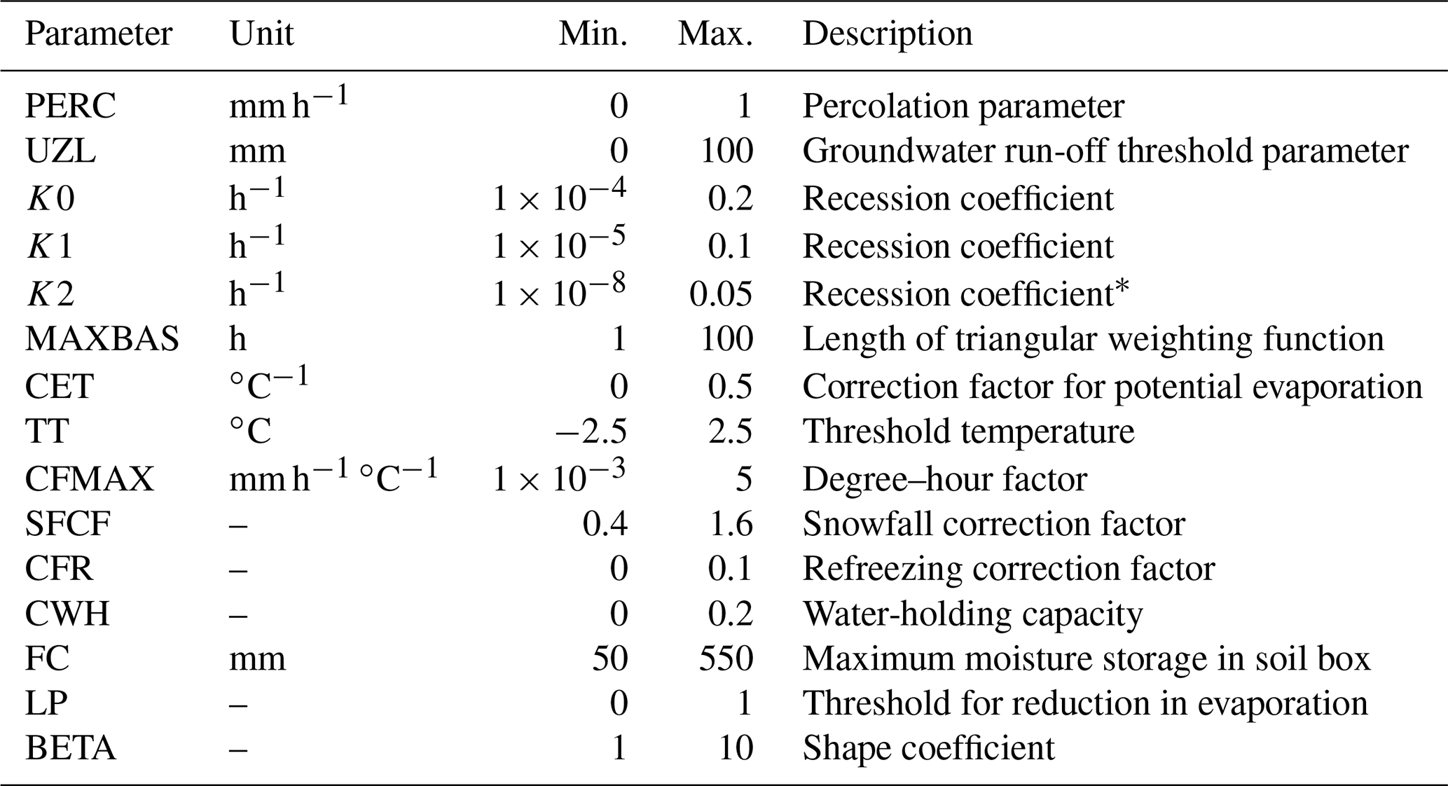
^* For recession coefficients the following condition must be fulfilled: $K\mathrm{0}>K\mathrm{1}>K\mathrm{2}$.

Appendix B: Equations used in the multi-objective function

$$\begin{array}{}\text{(B1)}& R_{\mathrm{KGE}}=\mathrm{1}-\sqrt{(r-\mathrm{1}{)}^{\mathrm{2}}+(\mathit{\alpha }-\mathrm{1}{)}^{\mathrm{2}}+(\mathit{\beta }-\mathrm{1}{)}^{\mathrm{2}}},\end{array}$$

where r, α and β are the correlation, a measure of the relative variability in the simulated and observed values, and a bias.

$$\begin{array}{}\text{(B2)}& R_{\mathrm{PEAK}}=\mathrm{1}-{\displaystyle \frac{\sum {\left(Q_{\mathrm{o},\mathrm{peak}}-Q_{\mathrm{s},\mathrm{peak}}\right)}^{\mathrm{2}}}{\sum {\left(Q_{\mathrm{o},\mathrm{peak}}-{\stackrel{\mathrm{‾}}{Q}}_{\mathrm{o},\mathrm{peak}}\right)}^{\mathrm{2}}}},\end{array}$$

where Q_o,peak and Q_s,peak are observed and simulated values for flood peaks, and ${\stackrel{\mathrm{‾}}{Q}}_{\mathrm{o},\mathrm{peak}}$ is the average value of Q_o,peak.

$$\begin{array}{}\text{(B3)}& R_{\mathrm{MARE}}=\mathrm{1}-{\displaystyle \frac{\mathrm{1}}{n}}\sum {\displaystyle \frac{|Q_{\mathrm{o}}-Q_{\mathrm{s}}|}{Q_{\mathrm{o}}}},\end{array}$$

where n is the number of observation points, and Q_o and Q_s are observed and simulated discharge.

For further details on R_KGE see the work of Gupta et al. (2009), for details on R_PEAK see the work of Seibert (2003), and for details on R_MARE see the work of Dawson et al. (2007).

Appendix C: Model calibration results

The optimized hydrological-model parameter sets are presented in Fig. C1, whereas diagnostics of the model performance during the calibration and validation periods are presented in Fig. C2.

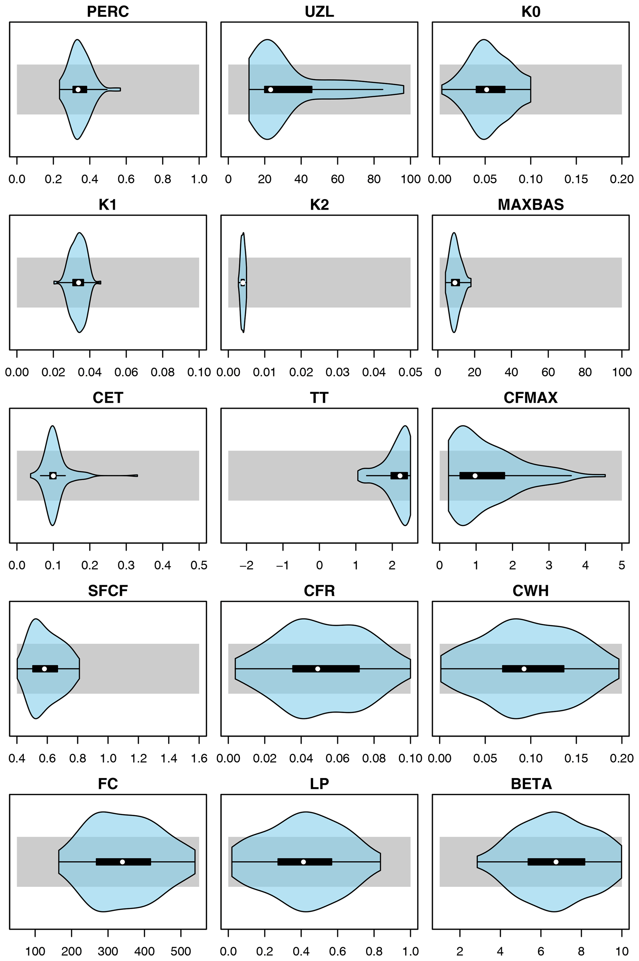
Figure C1 Violin plots (blue) summarizing 100 optimized parameter sets of the HBV model for the Dünnern at Olten catchment vs. initial calibration ranges (grey). Units as in Table A1.

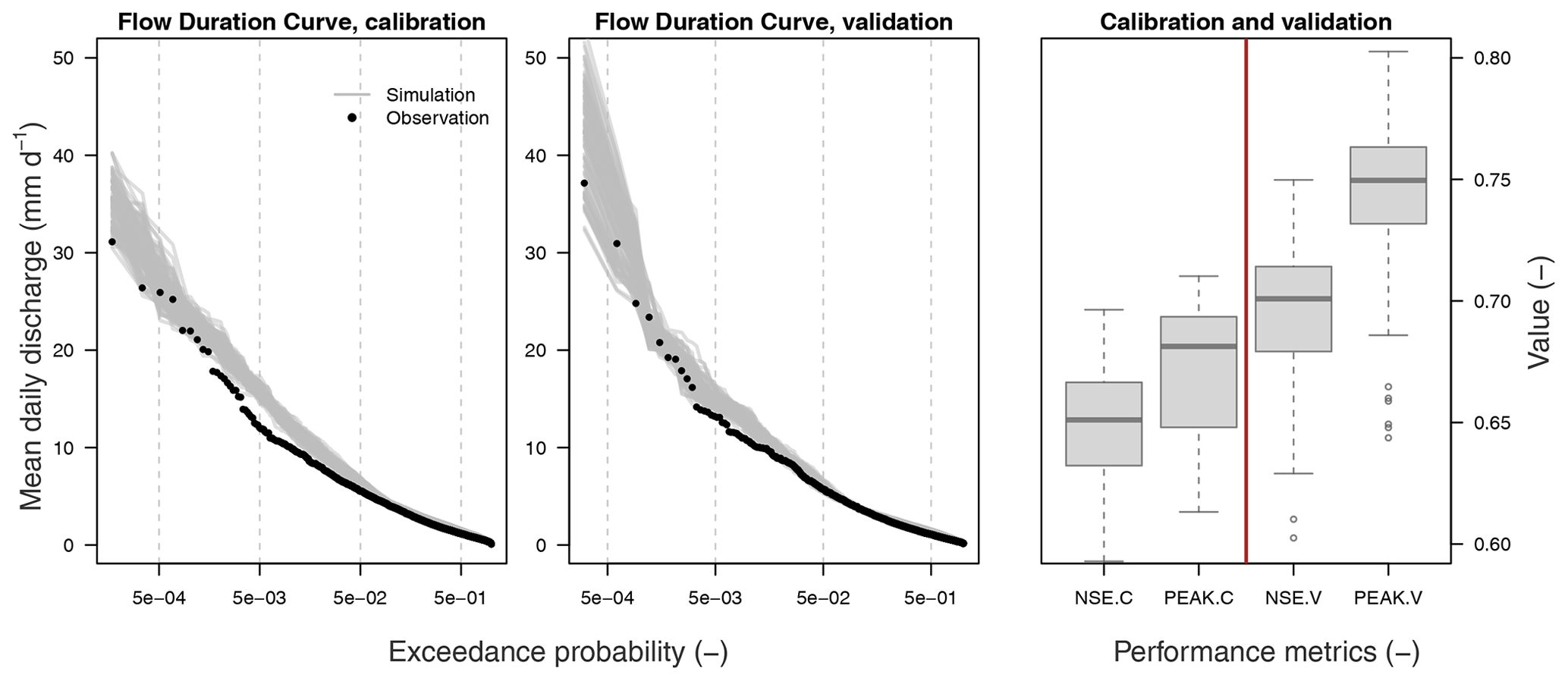
Figure C2 Flow duration curves and model performance metrics for calibration and validation periods over all 100 optimized parameter sets.

Appendix D: Scenario variability

The variability in the precipitation depth (annual daily maxima) and temperature (annual daily minima and maxima) of 100 meteorological scenarios used in this study is presented in Fig. D1. It can be seen that, in comparison to the observations, the meteorological scenarios are generally slightly colder (μ=22.9 ^∘C and σ=1.5 ^∘C vs. μ=25.8 ^∘C and σ=1.4 ^∘C for the annual daily maxima and $\mathit{\mu }=-\mathrm{11.9}$ ^∘C and σ=3.1 ^∘C vs. $\mathit{\mu }=-\mathrm{7.3}$ ^∘C and σ=3.5 ^∘C for the annual daily minima) and wetter (μ=46.1 mm and σ=12.4 mm vs. μ=45.9 mm and δ=12.0 mm for the annual maximal daily precipitation depths). The variability in resulting hydrological scenarios is presented in Fig. D2 together with observations.

Figure D1 Variability in 100 meteorological scenarios used in this study vs. observations.

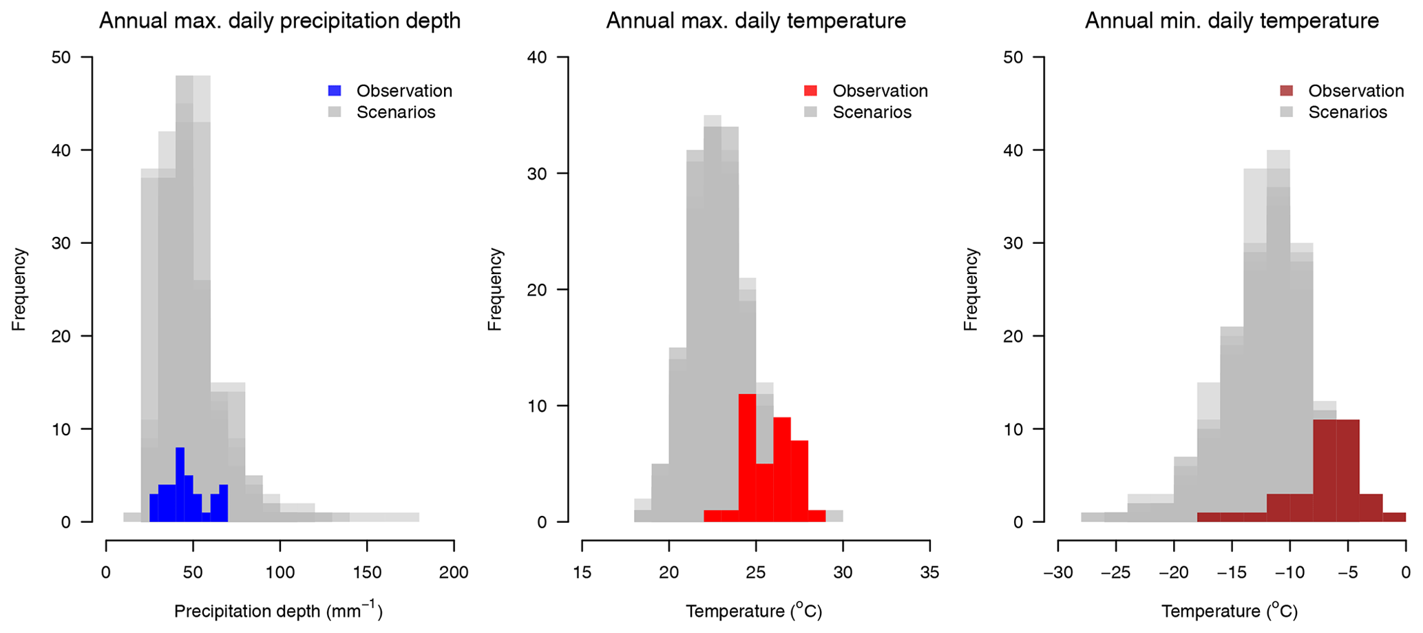
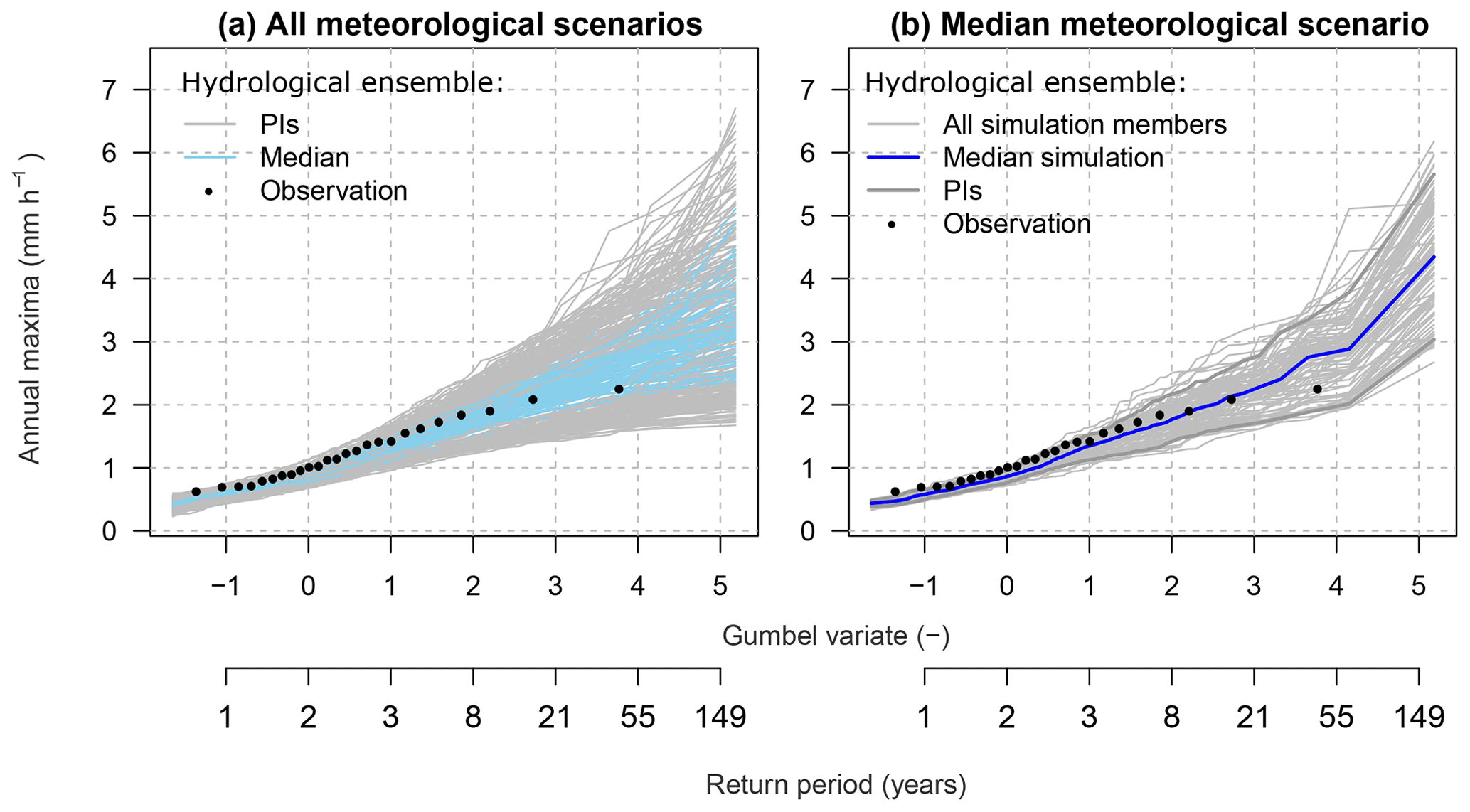
Figure D2 Variability in 100 hydrological scenarios used in this study; (a) hydrological ensemble with all meteorological scenarios and all hydrological-model parameters; (b) hydrological ensemble with all hydrological-model parameters but for the median meteorological scenario only. PIs represent the 90 % predictive intervals.