the Creative Commons Attribution 4.0 License.
the Creative Commons Attribution 4.0 License.
 | 17 Dec 2020
The potential of Smartstone probes in landslide experiments: how to read motion data
J. Bastian Dost
Oliver Gronz
Markus C. Casper
Andreas Krein
Laboratory landslide experiments enable the observation of specific properties of these natural hazards. However, these observations are limited by traditional techniques: frequently used high-speed video analysis and wired sensors (e.g. displacement). These techniques lead to the drawback that either only the surface and 2D profiles can be observed or wires confine the motion behaviour. In contrast, an unconfined observation of the total spatiotemporal dynamics of landslides is needed for an adequate understanding of these natural hazards.
The present study introduces an autonomous and wireless probe to characterize motion features of single clasts within laboratory-scale landslides. The Smartstone probe is based on an inertial measurement unit (IMU) and records acceleration and rotation at a sampling rate of 100 Hz. The recording ranges are ±16 g (accelerometer) and ±2000∘ s−1 (gyroscope). The plastic tube housing is 55 mm long with a diameter of 10 mm. The probe is controlled, and data are read out via active radio frequency identification (active RFID) technology. Due to this technique, the probe works under low-power conditions, enabling the use of small button cell batteries and minimizing its size.
Using the Smartstone probe, the motion of single clasts (gravel size, median particle diameter d50 of 42 mm) within approx. 520 kg of a uniformly graded pebble material was observed in a laboratory experiment. Single pebbles were equipped with probes and placed embedded and superficially in or on the material. In a first analysis step, the data of one pebble are interpreted qualitatively, allowing for the determination of different transport modes, such as translation, rotation and saltation. In a second step, the motion is quantified by means of derived movement characteristics: the analysed pebble moves mainly in the vertical direction during the first motion phase with a maximal vertical velocity of approx. 1.7 m s−1. A strong acceleration peak of approx. 36 m s−2 is interpreted as a pronounced hit and leads to a complex rotational-motion pattern. In a third step, displacement is derived and amounts to approx. 1.0 m in the vertical direction. The deviation compared to laser distance measurements was approx. −10 %. Furthermore, a full 3D spatiotemporal trajectory of the pebble is reconstructed and visualized supporting the interpretations. Finally, it is demonstrated that multiple pebbles can be analysed simultaneously within one experiment. Compared to other observation methods Smartstone probes allow for the quantification of internal movement characteristics and, consequently, a motion sampling in landslide experiments.
- Article
(7435 KB) - Full-text XML
-
Supplement
(17681 KB) - BibTeX
- EndNote


The spatiotemporal progression of moving slope material is the subject of research in various geoscientific disciplines (e.g. Wang et al., 2018; Aaron and McDougall, 2019; Schilirò et al., 2019). Laboratory experiments are a well-established instrument to investigate the physical behaviour of landslide motion processes. However, the observation of internal characteristics of a moving landslide mass poses a critical challenge. Nevertheless, an exact description of the internal behaviour is crucial to understand the mobility of these natural phenomena. The present study introduces an autonomous and wireless measuring device to observe the spatiotemporal motion of single clasts within a moving landslide mass in laboratory experiments.
1.1 Experimental investigation of landslide processes
To understand the physics of both dry and fluid-containing landslide processes on different scales and velocities, multitudinous experimental studies were undertaken during the last decades. For instance, Davies and McSaveney (1999) reproduced dry granular avalanches and concluded that the extraordinary spreading of very large granular avalanches may be caused by phenomena like rock fragmentation. Okura et al. (2000) conducted outdoor experiments to investigate the runout behaviour of rockfalls. They found that even though the centre of mass moved over shorter distances, the frontal part of the rockfall body spread over a larger area. In addition, they observed by means of a visual particle-tracking method that individual blocks did not change their relative positions during the motion process. This means that frontal blocks were deposited in a distal zone. To explain these findings, Okura et al. (2000) argued that the frontal blocks gain additional dissipation energy because of clast collisions within the rockfall body. In contrast, rear blocks lost energy due to the collisions. Beyond that, Manzella and Labiouse (2009, 2013) investigated the influence of randomly or orderly stored blocks prior to the material release of artificial granular landslides. This contrasting initial condition was used as an indicator for fragmentation. They found that the potential internal and external friction strongly influence the energy dissipation during the displacement process. For instance, if the bricks are stored randomly (high grade of fragmentation) or a sharp slope break exists (induces fragmentation), frictional and collisional conditions are pronounced, and energy dissipation is intensified. In turn, this results in a strong spreading of the material.
These studies have in common that the displacing material is considered as one body changing its shape. Thereby, the motion process is observed from the outside, and conclusions of the internal behaviour are drawn indirectly. This is a consequence of limited observation techniques. By means of (high-speed) video analysis, such as particle image velocimetry (PIV) or the so-called fringe projection method (e.g. Manzella, 2008), only the surface or transversal sections of the body can be analysed. To overcome these restrictions, several methods were developed for the internal measurement of motion characteristics. For instance, Yang et al. (2011) presented a detection system for impact pressure within debris flows and subsequently calculated the internal velocity. Additionally, wired devices such as piezometers, load cells and sensors for pore water pressure and deformation are common instrumentations for landslide experiments of various scales and objectives (e.g. Moriwaki et al., 2004; Ochiai et al., 2007; Ried et al., 2011).
Microelectronic devices for motion detection became common during the last years. Experimental studies use acceleration sensors of micro-electro-mechanical systems (MEMSs) or combined acceleration and rotation instruments such as inertial measurement units (IMUs). After the early works of Ergenzinger et al. (1989) and Hanisch et al. (2003), who developed an intelligent boulder equipped with multiple sensors, sensor technology became more accessible and cheaper during the last decade. Several studies focussed on technical aspects (i.e. hardware and software development) of so-called “smart tracers” used to investigate natural transport processes (e.g. Spazzapan et al., 2004; Cameron, 2012). Others applied these techniques to geoscientific or geotechnical questions, such as the impact of waves on armour units of breakwaters (e.g. Hofland et al., 2018). Volkwein and Klette (2014) presented a relatively large probe that could be embedded into boulders to record movement parameters of rockfalls. Although acceleration and rotation were recorded with high sampling rates to capture hard impacts of the rock, a further processing of the data was not carried out. The position of the rock during the displacement was tracked via a WLAN (wireless local area network) connection. Another recent example of sensor techniques to describe gravitational-induced movements is the Smart Soil Particle (SSP) presented by Ooi et al. (2014). Although acceleration data were interpreted quantitatively, a derivation of movement characteristics of the landslide motion was not performed. Additionally, the SSP needs wires for energy supply and data transmission, and these wires confine a free movement of the device within the soil.
The need of an autonomous and wireless device to investigate geomorphic transport processes was recently identified by Spreitzer et al. (2019). They presented a sensor-based probe to monitor the movement of artificial tree trunks during laboratory-scale flood experiments. Although a qualitative interpretation of the transport behaviour was done, a further processing of the data and a reconstruction of the trunks' trajectories were not carried out. Because under flood conditions, wood is mostly transported at the water table level, the trajectory can be followed visually. In terms of landslide processes, this might not be possible. Here, it is of great importance to track material components that are embedded within the moving landslide body.
1.2 Scope of the present study
The present study introduces the Smartstone probe v2.0 as a device to measure movement characteristics of single clasts in situ within a surrounding mass. Thereby, methodological and technical progress compared to the former probe version, presented by Gronz et al. (2016), will be demonstrated. An experimental setup was developed that reproduces artificial landslides of a dry granular flow type. The experimental design focussed on sensor application and not on natural landslide reproduction. The Smartstone probe is the object of investigation in the present study. Photo and video documentation as well as reference measurements were carried out to verify the results (see Sect. 2). The present study deals with the following aspects:
-
There has been a significant technical improvement since Gronz et al. (2016) introduced the first version of the Smartstone prototype. Therefore, one objective is the description of the recent Smartstone probe. In addition, we document major changes to the former version and the corresponding technical specifications.
-
Beyond that, we explain additional information that is supplied by smart sensors and illustrate the specific properties of motion data. Based on a quantitative interpretation, we give an introduction how to read motion data in terms of flume-scale landslide movements.
-
Subsequently, we demonstrate how physical movement characteristics can be derived from the measured and calibrated data and in what way they are different.
-
Further, we highlight the potential of a 2D and 3D visualization of the paths a clast took during the movement and how these visualizations allow for an easy recognition of complex motion patterns.
-
Finally, we investigate the limitations of the Smartstone prototype and discuss what developments will be necessary to improve the probe and data handling further.
2.1 The Smartstone probe v2.0
In the present study, motion processes of single clasts were mainly observed by means of the Smartstone probe v2.0. The current prototype version is an improvement of the device that was presented by Gronz et al. (2016). A summary of the recent technical specifications is given in Table 1. All Smartstone kit components necessary to control the probe are shown in Fig. 1a. Contrary to the former version, which used a metal casing, the recent probe consists of an approx. 55 mm long and 10 mm wide plastic tube that holds the entire hardware. Therefore, the former external antenna could be replaced by an internal antenna, which allows for an easier handling under experimental conditions. Energy is supplied by a single 1.5 V button cell battery (type AG5). Two plastic plugs enable a waterproof closing. In the standard configuration, the plugs have two sealing lips. Under dry conditions, plugs with only one sealing lip can be used as well, reducing the probe's total length to approx. 50 mm.
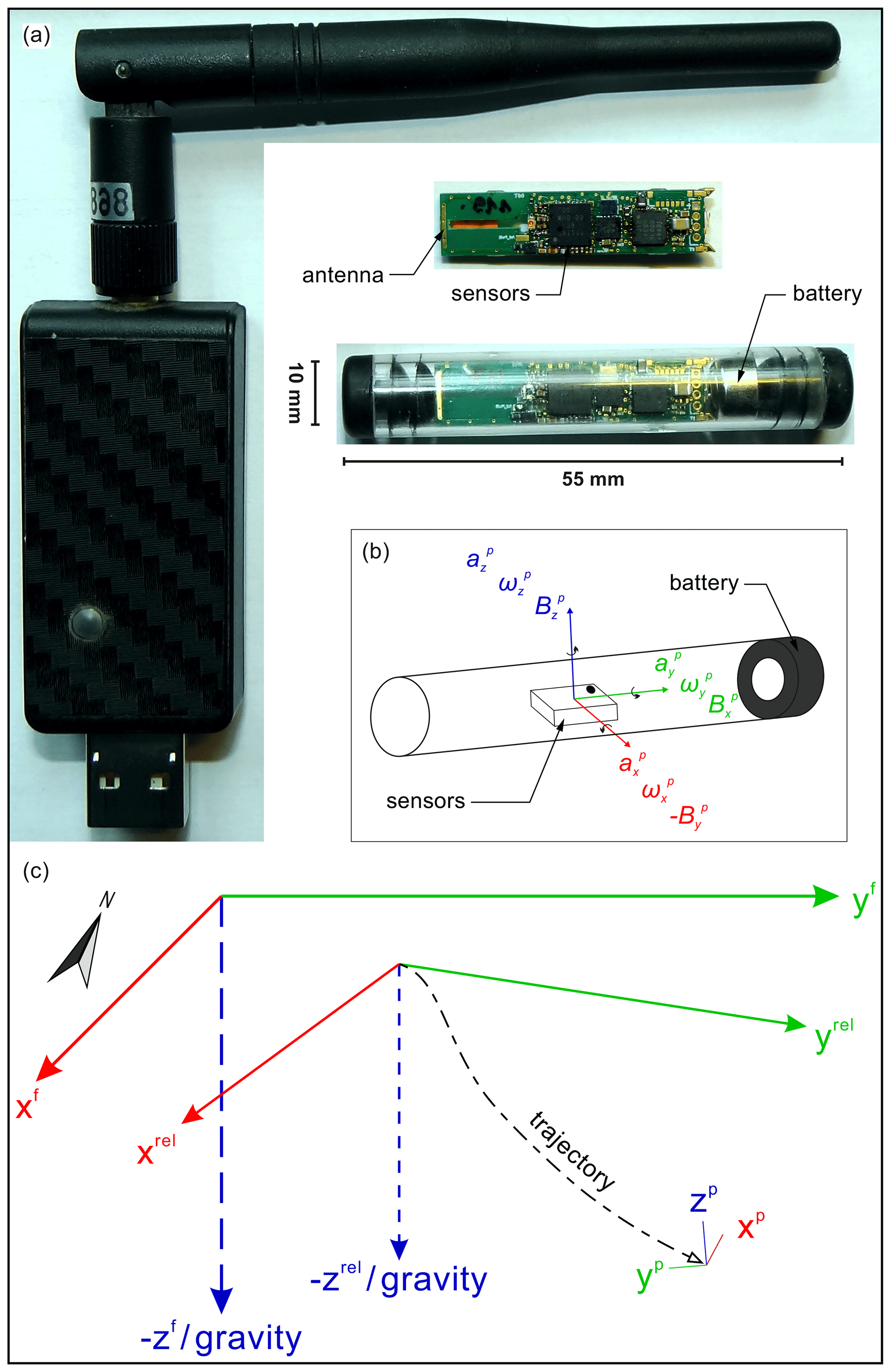
Figure 1Smartstone v2.0 hardware kit and technical conventions. (a) Hardware components including a USB gateway with an antenna for communication between a computer and the probe. Electronic components within a plastic tube, hosting the triaxial sensors (compare Table 1) and the internal antenna. (b) Axis conventions of the Smartstone probe v2.0. (c) Reference systems as used in the present study.
Table 1Technical specifications of the Smartstone probe v2.0 as provided by Bosch Sensortec GmbH (2014, 2015) and manufacturer information from Smart Solutions Technology GbR.
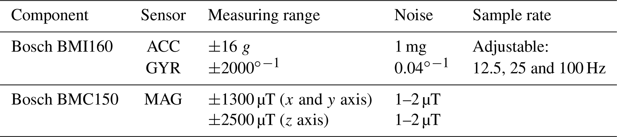
The centrepiece of the probe is the approx. 30 mm long conductor plate holding an IMU with a combined accelerometer (ACC) and gyroscope (GYR) sensor – the Bosch BMI160 (Bosch Sensortec GmbH, 2015). The 16 bit triaxial ACC measures accelerations (a) within the range of ±16 g which strongly enhances the recording range comparing ±4 g of the former version (g as the unit for gravitational acceleration). It exhibits a noise level of 1 mg at 100 Hz sampling rate. The 16 bit triaxial GYR measures rotations in terms of angular velocity (ω) within the range of ±2000∘ s−1 at a noise level of 0.04∘ s−1. The IMU is placed in the centre of the conductor plate. In addition, the probe is equipped with a magnetic sensor (“e-compass”, MAG). For this purpose, the Bosch BMC150 (Bosch Sensortec GmbH, 2014) is used to record within the range of ±1300 µT (x and y axes) and ±2500 µT (z axis). Depending on the measuring range, the noise level is between 1 and 2 µT (the earth's magnetic field strength ranges between 22 and 67 µT). Sensor data and corresponding timestamps are stored in internal 1 MB memory.
To allow for an undisturbed motion, the Smartstone probe was developed as a wireless and autonomous instrument. The entire communication between the probe and a control software is performed by active radio frequency identification (active RFID) via the 868 MHz band. Contrary to other communication techniques (such as WLAN), active RFID works under low-power conditions, enabling the use of small batteries for its energy supply. Additionally, it offers a higher operation range compared to Bluetooth. Because of this low-power communication technique, the total size of the probe can be minimized. A USB gateway works as the interface between the probe and the controlling software with a graphical user interface (GUI). This enables the adaptation of probe settings, start of recording and data readout. For instance, a recording threshold can be set to avoid minor signals (e.g. vibrations due to environmental perturbations) filling the internal memory before the considered motion begins. Moreover, single sensors can be switched off, and the sampling rate can be adjusted (see Table 1). These settings will influence the time until the internal memory is completely filled. For instance, using all sensors (ACC, GYR and MAG) at a sampling rate of 100 Hz fills the memory in approx. 8 min of continuous measurement.
The previously mentioned probe dimensions were chosen because the probe should be embedded into representative clasts of the investigated material (see below). For this reason, a small button cell was used, being aware that its capacity is limited. Yet, the Smartstone probe hardware could also be used to investigate the motion of larger objects. Hence, longer plastic tubes and larger batteries (type AAAA) could be used for this propose. For the present study, five probes were used, whereof one was damaged and could not be included in the analysis (see below).
2.2 Axis conventions and reference systems
The following notations and conventions have to be considered during data description and interpretation. Due to the triaxial architecture, sensor data are supplied by a triplet of values in each time step. The triplet represents a vector with three space components (Fig. 1b). For instance, the ACC reading is composed of , and , where the subscript denotes the axis and the superscript indicates that the values are probe readings (compare also Fig. 1c). Note that ACC and GYR are mounted on one side of the conductor board, resulting in the same axis configurations. Contrarily, the MAG is mounted on the opposite side of the conductor board (rotated by 180∘). Therefore, its x and y axis are also rotated. Following the right-hand rule, positive rotational directions are indicated by small curved black arrows.
To compare relative movement characteristics like distance or velocity of different probes, the inner data–coordinate system p must be transformed into an outer reference system rel (Fig. 1c). The simplest way to do this is the construction of a reference system using the probe's starting position as the coordinate origin. The system is defined by the sensor's inner coordinate system of the first time step rotated so that the z axis follows gravity. The axes of this relative (to the starting position) outer coordinate system are donated with xrel, yrel and zrel. After the motion has started, the probe's inner orientation will change, while the outer reference system keeps its axis configuration. Consequently, within this reference system, it is possible to calculate the probe’s orientation and the covered distance in each time step. In Fig. 1c for instance, the probe has changed its orientation significantly compared to its starting position while moving along the assumed trajectory.
However, the different probe-specific outer coordinate systems must be transformed into the same local reference system to compare different probes' trajectories. For the present study, this local reference system is oriented towards the experimental flume (see Sect. 2.4). Following the former conventions, the axes were donated as xf, yf and zf. Note that the axes orientations of the outer (rel) and the local reference system (f) may not be identical, except for zrel and zf, as they follow gravity.
In different applications, where a global positioning is required, reference points of the outer coordinate systems must be known in the global system to determine the absolute probe position in the global system.
2.3 Data calibration and processing
Prior to the calculations of movement characteristics, sensor data have to be calibrated. As further data processing uses ACC readings to derive movement characteristics, calibration is essential for the ACC. The recorded acceleration values of each axis (, , ) are generally erroneous due to two reasons: (i) a (quasi-)constant misreading, as the mass inside the sensor, which moves to measure acceleration, is not precisely equal in all sensors (manufacturing tolerance), resulting in a bias as well as a linear scaling of true values, and (ii) the imprecise orthogonal alignment of the sensor axes and crosstalk, meaning that a fraction of each axis acceleration will result in readings at the two other axes. Both of them can be corrected by adding a sensor- and environment-depending vector (i) to the readings and multiplying them with a scale factor matrix (ii).
Frosio et al. (2009) describe an optimization algorithm that estimates these error components simultaneously. In the present study this approach was applied for the first time on Smartstone probe data. Because one probe was somehow damaged during the experiments, ACC data of the remaining four probes were calibrated by means of the optimization algorithm using MATLAB software. Subsequently, only these probes were analysed.
By means of the recorded acceleration and rotation data, the movement characteristics and the probe's trajectory can be reconstructed. Basically, these calculations use Newton's physical laws and integration of the recorded accelerations. Practically, if the pebble is in motion, gravitational acceleration and acceleration due to the motion will interfere. Nevertheless, position and orientation in each time step can be estimated by combining the ACC and GYR readings. This approach is termed sensor fusion (e.g. Koch, 2014). In the present study a quaternion-based estimation algorithm was used that was originally developed to track the human gait. It was adapted from Madgwick et al. (2011) and x-io Technologies (2013) and supplies the movement characteristics velocity v and displacement s relative to the starting position. Additionally, it enables a 3D visualization of the trajectory. For a detailed description of the computation see Sect. 3.2.
2.4 Experimental setup
The experimental setup was designed regarding the following requirements: (i) an exact and rapid triggering mechanism, (ii) multiple repetitions with identical boundary conditions due to homogeneous and dry material, and (iii) flexibility for future studies. Figure 2a shows the configuration that was used for the present study. A spring-based triggering mechanism allowed a rapid release of the material stored in a box on top of the flume. Eight single springs supplied a total spring force of approx. 1660 N. After the release, the material moved along an approx. 4.2 m long plane inclined by 20∘. Some clasts also reached the lower part of the flume, which is inclined by 10∘. Lateral barriers limited the width of the flume to approx. 2.2 m. The bottom of the flume was covered by a dimpled sheet to provide uniform basal frictional conditions.
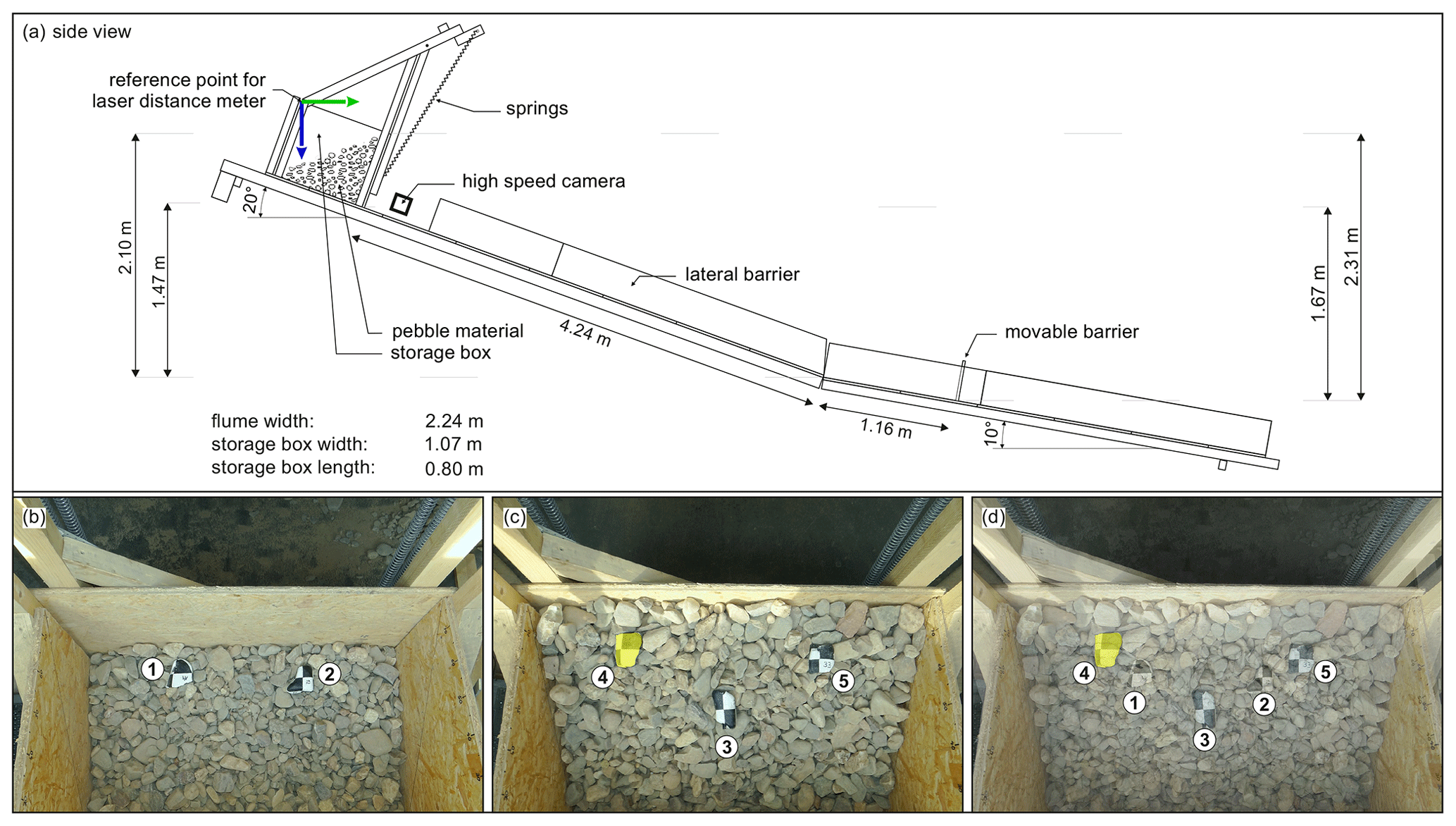
Figure 2Experimental setup. (a) Simplified sketch of the laboratory flume. Green and blue arrows mark axes of the flume reference system in the yf and zf direction, respectively. (b–d) Starting positions of the five equipped embedded (b) and superficial (c) pebbles. (d) Overlay of (b) and (c) showing the initial positions of all equipped pebbles prior to the experiment. Pebble 4, whose data were plotted in Figs. 3 to 5, is highlighted in light yellow in (b) and (d). Note that pebble 5 could not be included in the analyses due to its damage.
A high-speed camera was placed close to the storage box to document the initial motion of the material. A Optronis CR4000x2 camera and a Tamron XR Di II (17–55 mm, 1:2.8) lens were used. High-speed sequences were recorded at 500 fps (frames per second) with a resolution of 2304×1720 pixels and were stored as *.jpeg files. The camera was mounted with an inclination of 20∘ on the left side of the flume (direction of motion). The recorded pictures were mirrored during post-processing to achieve a better comparability between high-speed sequences and probe data. Therefore, motion proceeds from left to right in all attached figures and the supplementary high-speed video (Video 1). The video facilitates the verification of the interpretation (if the pebble is visible) of the sensor data and the concluded motion modes. We will refer to it several times.
For the present study, a uniformly graded pebble material of fluvial origin (fluvial deposit of Moselle river) was used. Lithologically, it mainly consists of quartzite with smaller portions of greasy quartz and slate. Therefore, pebbles are laminated and rounded to well-rounded shapes. The particle size range was specified to 32 to 63 mm, and the effective unit weight amounts to 1.55 t m−3 (manufacturer information; EIDEN, 2017). A median particle diameter d50 of 42 mm and a uniformity coefficient CU of 2.1 was determined by sieving analysis. Clasts with diameters ⩾60 mm amount to approx. 12 % (w/w; weight to weight) of the material. A total mass of approx. 520 kg was used for the present study.
From the material several pebbles were taken to be equipped with Smartstone probes. For this purpose, a hole was drilled through the pebble and modified in the way that a snug fit of the probe was achieved. Therefore, the probe could not move within the hole during the motion process. Additionally, the pebbles were marked and numbered to be easily identified in the high-speed sequences. The specific unit weight of each prepared pebble was determined by immersion weighing before and after the preparation procedure. In this study, a detailed analysis of quarzitic pebble 4 will be carried out. By means of immersion weighing a change in density (2.66 g cm−3) was not detectable.
The storage box was filled with about 50 % of the material prior to the experiment. Two probe-equipped pebbles were placed, and their position was measured at the temporal surface as displayed in Fig. 2b. Afterwards, more pebble material was filled into the storage box, and three more equipped pebbles were placed at the final surface. Figure 2c and d show the initial conditions prior to the experiment. The positions of each equipped pebble were additionally measured relative to the upper edge of the storage box. This was done using a laser distance meter (accuracy of ±1 mm). Measures were conducted for the yf and zf direction for both the starting and the depositional position.
Hereinafter, Smartstone probe data of one experiment were chosen to present (i) sensor recordings (Fig. 3), (ii) the derived movement characteristics (a, v and s, Fig. 4), and (iii) 2D and 3D visualizations (Figs. 5 and 6). The latter illustrate the complex motion trajectory of a single pebble within the landslide mass. Subsequently, data of one pebble are analysed (Sects 3.1 to 3.3) before the motion of multiple pebbles is considered in Sect. 4.1.
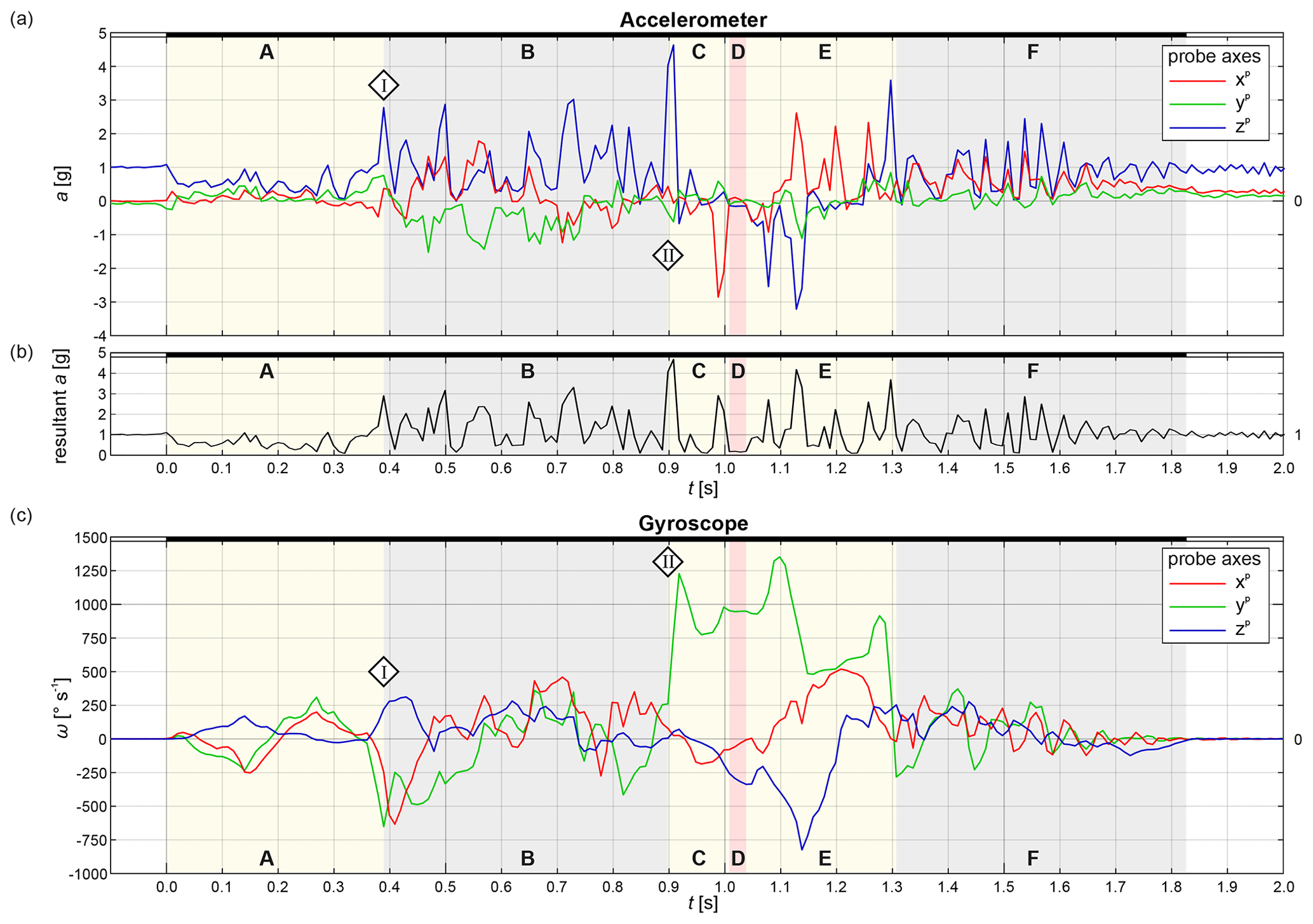
Figure 3Calibrated sensor data of pebble 4. Data are plotted versus relative time since the start of motion. Stationary periods are indicated by white bars, and motion is indicated by a black bar at the top of each plot, respectively. Vertical bars in light yellow, grey and red mark particular phases (A–F) within the motion sequence (for description see text). Numbered diamonds indicate distinct points in time (see also Fig. 4). (a) ACC data, (b) resultant acceleration magnitude and (c) GYR data. Curves in (a) and (c) show recordings along and around each probe axis, respectively.
3.1 Qualitative description and interpretation of probe data
Figure 3 shows the calibrated data of pebble 4. For this test, only acceleration in g (1 g = 9.81 m s−2, Fig. 3a) and rotation in ∘ s−1 (Fig. 3c) were recorded. Note that the three curves of xp, yp and zp (Fig. 3a) show the acceleration along the particular axis (see below). The gyroscope data curves (Fig. 3c) show rotation around these axes. At the top of each plot, white bars indicate stationary (no motion) periods, and black bars indicate non-stationary (motion) periods. The previously explained data processing (see Sect. 2.3) was only applied to non-stationary periods. The whole motion sequence can be subdivided into six phases (A to F) with distinct properties characterizing a specific motion behaviour. Additionally, two discrete time points (diamond I and II) indicate major changes within the motion sequence. These phases and time markers highlight the same events in Figs. 3 to 5 and the supplementary video.
The data sequence of pebble 4 covers a total duration of 2.1 s. The start of motion of pebble 4 was set to 0.0 s. Before the actual motion begins (stationary conditions, left white bars in Fig. 3), low values were recorded along xp and yp, though xp readings are on a slightly higher level (approx. 0.0 g). At yp, low negative values were recorded. Only at zp can higher values of approx. 1 g be seen. This pattern represents non-motion conditions, where only gravitational acceleration is recorded. This assumption is supported by the zero readings of the GYR. The plot of Fig. 3b shows that the resultant acceleration is approx. 1 g. According to the conventions from Sect. 2.2, can be written as
Each axis reading reflects a fraction of the gravity vector and is given by
where α, β and γ define the angle between xp, yp, zp and the gravity vector, respectively. Accordingly, under static conditions the probe's orientation relative to the gravity vector (vertical direction) can be calculated from the three readings of , and .
3.1.1 Phase A (light-yellow shading)
A sudden change in the axis readings at 0.0 s is visible in all three plots. Between 0.0 and approx. 0.03 s, a clear drop of zp recordings to half of the former level is visible in the acceleration plot (Fig. 3a). Simultaneously, the values of xp increase slightly above zero, and those of yp slightly decrease1. Generally, relatively low acceleration readings are visible on all three axes during phase A, reflected by the resultant acceleration (Fig. 3b). Low absolute values of acceleration can only be achieved if free fall (unconfined acceleration within the earth's gravitational field into the direction of its centre of mass) is mixed with an additional. Thus, values between 0 and 1 g imply a hampered free fall (no completely developed free fall, confined motion) and/or an additional lateral acceleration.
In phase A the resultant acceleration is between zero and one. Hence, the pebble moved more or less downwards but was not in free fall. In fact, it was confined by the surrounding mass (see below). During phase A, angular velocities of about ±250∘ s−1 are visible in Fig. 3c. It is conspicuous that between 0.0 and approx. 0.2 s, negative values are visible on xp and yp, while zp shows positive values. Between approx. 0.2 and 0.38 s, oppositional axis configurations with low absolute values at zp and positive angular velocities at xp and yp are displayed. These features show a forward and backward rotation of the pebble mainly around xp and yp. Generally, phase A is characterized by relatively smooth curves without any large peaks and comparably low sensor readings for both the ACC and the GYR. Thus, it appears that during this phase, a relatively calm motion behaviour was present without any stronger collisions between pebble 4 and the surrounding clasts. We conclude that the surrounding part of the mass moves coherently downwards.
3.1.2 Diamond I and phase B (light-grey shading)
At 0.389 s (diamond I) a distinct transition in the data sequence is visible. Contrary to phase A, uneven and peaky curves can be seen in all plots. In Fig. 3a, zp generally shows high acceleration peaks of approx. 3.0 g. Along yp, values around −1 g were recorded; along zp, values around 1 g were recorded from 0.389 to approx. 0.7 s. The resultant acceleration (Fig. 3b) also shows a peaky curve with values between 0.2 and approx. 3.0 g. Looking at the GYR data, high angular velocities of about 600∘ s−1 at xp and yp are visible around diamond I. This indicates a strong rotation around these axes and may be a hint for major changes in direction. After that, relatively low ω values <500∘ s−1 are recorded during phase B.
3.1.3 Diamond II and phase C (light-yellow shading)
At diamond II another strong transition is visible in the time series. The strongest peak of the whole sequence (approx. 4.6 g) is measured at zp for two subsequent readings. Thus, the change in velocity is bigger than all other changes, as the strongest absolute acceleration also lasts longer than most other acceleration peaks, which only consist of one reading. Because of the low acceleration recordings of xp and yp, the resultant acceleration is calculated to approx. 4.7 g. Diamond II introduces phase C, where higher sensor reading in GYR data are visible as well (Fig. 3c). Here, the phase begins with a relatively low ω value of approx. 260∘ s−1 at 0.898 s on yp. After that, a strong increase on yp is visible until at 0.918 s, a local maximum of approx. 1230∘ s−1, is reached. Interestingly, this peak was recorded after high values were recognized at , 0.01 s earlier. While the GYR readings of xp and zp are relatively low at approx. −150∘ s−1, values of yp stay at a high level of approx. 750∘ s−1. At the end of phase C, an increase of ω at yp is visible.
These recordings can be interpreted in the way that pebble 4 changes its mode from lateral sliding to rotation and saltation. This point in time is also clearly visible in Video 1 at the position marked with diamond II. In the following, each saltation is characterized by single strong peaks on different axes (as the pebble also rotates).
3.1.4 Phase D (light-red shading)
The short period between 1.008 and 1.038 s (four data samples) can be easily identified within the acceleration plots (Fig. 3a and b). Low ACC readings of all three probe axes led to a resultant a close to zero. As explained above, this is only possible under almost free-fall conditions. Therefore, it can be reasoned that the pebble 4 fell for approx. 0.03 s. The gyroscope plot (Fig. 3c) shows again high values of approx. 900∘ s−1 for yp and relatively low values for xp and zp. This implies a pronounced rotation while the pebble falls.
3.1.5 Phase E (light-yellow shading)
A strong rotation around yp continues at the beginning of phase E. But contrary to the former phases, and show increasing positive and negative values since approx. 1.07 s, respectively. At approx. 1.14 s a peak of ω of approx. −820∘ s−1 occurs at zp before the values decrease again. At about the same point in time, strong peaks are visible at the ACC readings at each probe axis. These lead to the second highest a resultant (approx. 4.2 g) of the whole time series. From approx. 1.23 to approx. 1.24 s another short period of ACC readings around zero is visible, resulting in an a resultant of approx. 0 g. At the end of phase E, a last strong a peak (3.6 g) at zp and a strong decline of the are visible. This denotes a major change in motion behaviour with a transition from strong rotations in phases C to E to less rotational but translational displacement.
3.1.6 Phase F (light grey) and the end of motion
During this last phase, a continuous decline of ω at all probe axes can be seen. Whereas values of approx. ±200∘ s−1 are recorded at approx. 1.3 s, until the end of the movement an almost logarithmic decrease of these values is visible. This decline appears also at the ACC readings from approx. 1.53 s onwards. At 1.826 s the end of the motion sequence is reached. GYR readings around 0∘ s−1 were recorded. At the ACC, only minor changes can be seen after this point in time. At zp values vary slightly below 1 g. Readings of xp and yp are slightly higher than 0 g. As the pebble is stationary, only the gravitational acceleration vector is displayed by the data. This is also visible in Fig. 3b, where the calculated a magnitude varies around 1 g.
Concerning the whole time series, some interesting aspects shall be mentioned: the small deviations from the mean axis readings of the ACC after the motion (right white bar) can be interpreted as oscillation of the flume construction after the impact. This is supported by the data pattern exhibiting uniform oscillations which are gradually decreasing in amplitude.
By comparing the ACC readings before and after the movement (white bars), a minor change of xp and yp can be seen. While xp showed values of ±0.0 g and slightly negative readings of yp before the start, low positive values were recorded after the motion on both axes. Contrary to this, zp shows slightly lower values after the motion compared to its readings before the start of the experiment. From this can be reasoned that the orientation of pebble 4 after the movement has changed. Because the stationary ACC readings of zp are slightly lower, it follows that this axis does not point exactly in the vertical direction after the motion. The probe is oriented in a different way than prior to the experiment.
Further, different “modes” of sensor readings occur during the motion sequence. The first mode is generally characterized by little ACC readings on all axes. In addition, the curves are relatively smooth and less peaky, which is particularly clear for the rotation data. This mode is present in phase A and for the short period of phase D. The second mode consists of peaky and relatively high acceleration values simultaneously with relatively low but peaky GYR readings. The amplitude of ACC values is relatively high. This mode occurs during phases B and F. Contrary, a third mode shows smoother (less peaky) ACC readings with lower amplitudes and high but less peaky GYR recordings. This mode can be observed in phases C and E. These oppositional observations reflect the previously mentioned motion behaviour. The first mode is recorded when the pebble mainly falls downwards and clast contact is inhibited. The second mode is recorded if translational transport under confined conditions occurs. Pebble 4 moves within the mass and is exposed to pronounced collisional contacts due to surrounding pebbles. This results in frequent impacts and, consequently, acceleration peaks. Because the pebble is generally not free to move, larger rotation is inhibited and minor but sudden orientation changes occur. This is reflected by the relatively low but peaky GYR readings. Contrary, the third mode occurs when the pebble rotates unconfined. This is only possible while the pebble is not surrounded by other material. This means that the pebble must be above the moving mass. In other words and geoscientifically speaking: the pebble saltates. This is also supported by the alternating pattern of high peaks and almost zero acceleration magnitude. This pattern results from saltation as the pebble bounces at the flume bottom before it rebounds and falls again.
3.2 Quantifying motion by means of derived movement characteristics
The previously explained data only focussed on the motion mode. In the following, the movement is investigated with respect to position and time. The recorded data are only a result of external influences (forces) that act on the pebble. However, from the recorded and calibrated data, the pebble’s movement characteristics relative to its staring position (arel, vrel and srel) can be derived by simple physical relations. The initial orientation of the pebble can be calculated according to Eqs. (1) and (2). By means of the received Euler angles α, β and γ, the sensor readings , and can be rearranged to , and (compare also Sect. 2.2). However, the representation by Euler angles may not be bijective and therefore may lead to an erroneous initial orientation (“gimbal lock”). Another method to derive initial orientation by means of acceleration and rotation data was presented by Madgwick et al. (2011). It is based on a quaternion representation and supplies bijective solutions (for detailed explanations the reader is referred to Madgwick et al. (2011) and specific literature such as e.g. Jazar, 2011). It was implemented into a MATLAB algorithm, which was published online at https://x-io.co.uk/gait-tracking-with-x-imu/ (last access: 3 August 2017) (CC license; x-io Technologies, 2013).
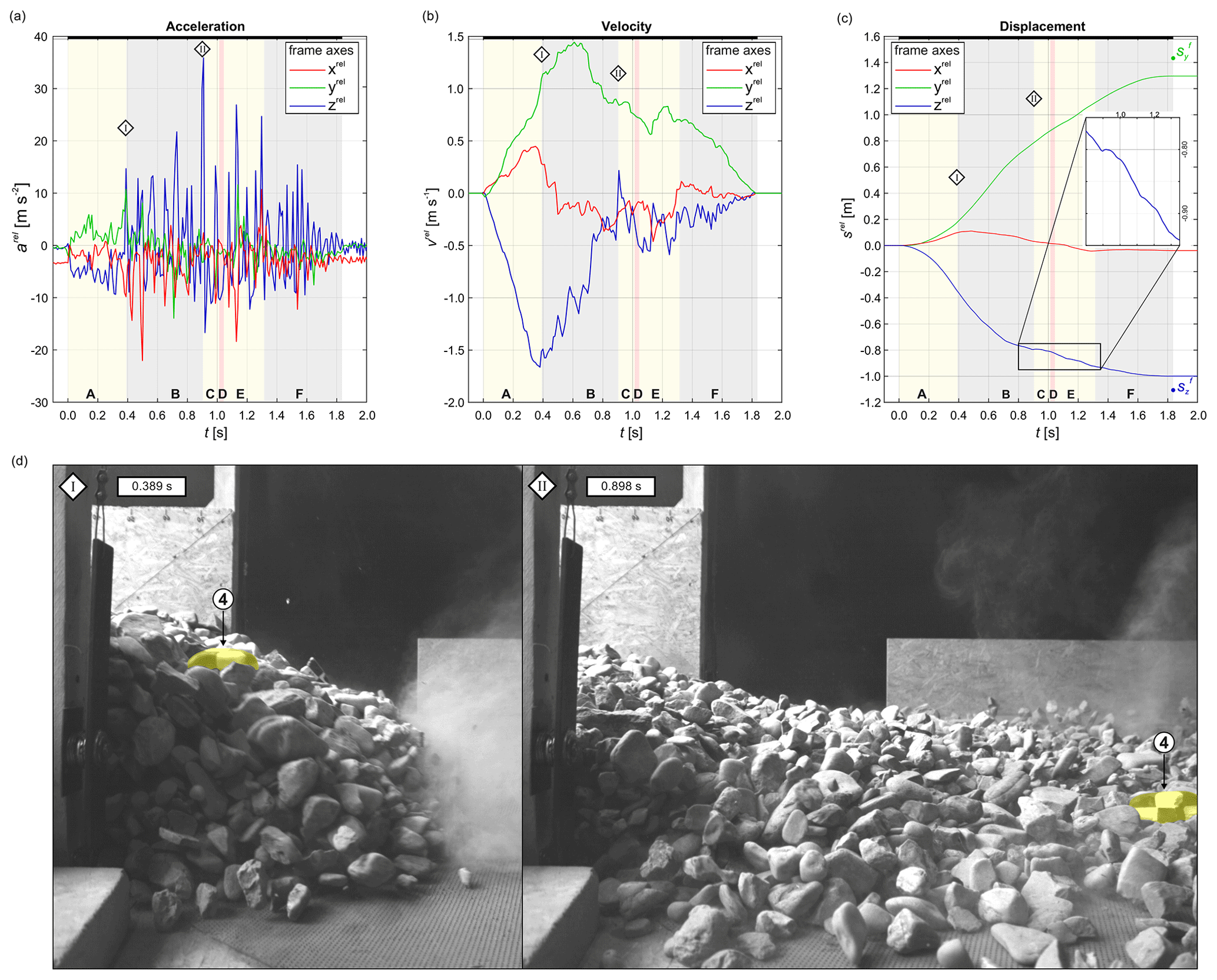
Figure 4Movement characteristics and high-speed captures. (a–c) Time series of the derived movement characteristics for (a) translational acceleration, (b) translational velocity and (c) translational displacement (with detail). The three curves in each plot give calculated time-dependent values for each axis of the relative reference system (as defined in Sect. 2.2). Motion phases and distinct time points are indicated as in Fig. 3. In (c) green and blue dots indicate the true displacement components in yf and zf directions measured by means of a laser distance meter (for explanation see Sect. 2.2). (d) High-speed captures at time points diamond I and II. The data of (a–c) were recorded with pebble 4, which is highlighted in light yellow and labelled in (d).
After finding the initial orientation, the vector arel consequently gives the translational acceleration of the pebble within a reference system relative to the pebble's staring position (compare Fig. 1c). Thereby, the direction of equals the gravity vector and thus points downwards. Hence, and give the horizontal component of arel. After the rearrangement of the recorded accelerations and with respect to time t, the movement characteristics vrel and srel can be obtained from the integration as
and
By applying these formula, movement characteristics were calculated for the non-stationary period and are plotted in Fig. 4a–c. Individual phases and distinct points in time are indicated in the same way as displayed in Fig. 3. Additionally, captures of the high-speed sequence from diamonds I and II are shown in Fig. 4d. Note also that acceleration values are plotted in units of m s−2. Data processing was applied from the start of motion (compare black bars in Figs. 3 to 5). Only arel was rearranged before the motion starts (white bars). During stationary periods these values are defective. This can be seen at xrel (Fig. 3a), where values of approx. −4 m s−2 were calculated. Obviously, this cannot be true as the pebble does not move. However, these false calculations are excluded from further integration (compare Fig. 3b and c) and do not influence the following interpretations. A summary of the finally derived distances that were covered by pebble 4 during each phase is listed in Table 2.
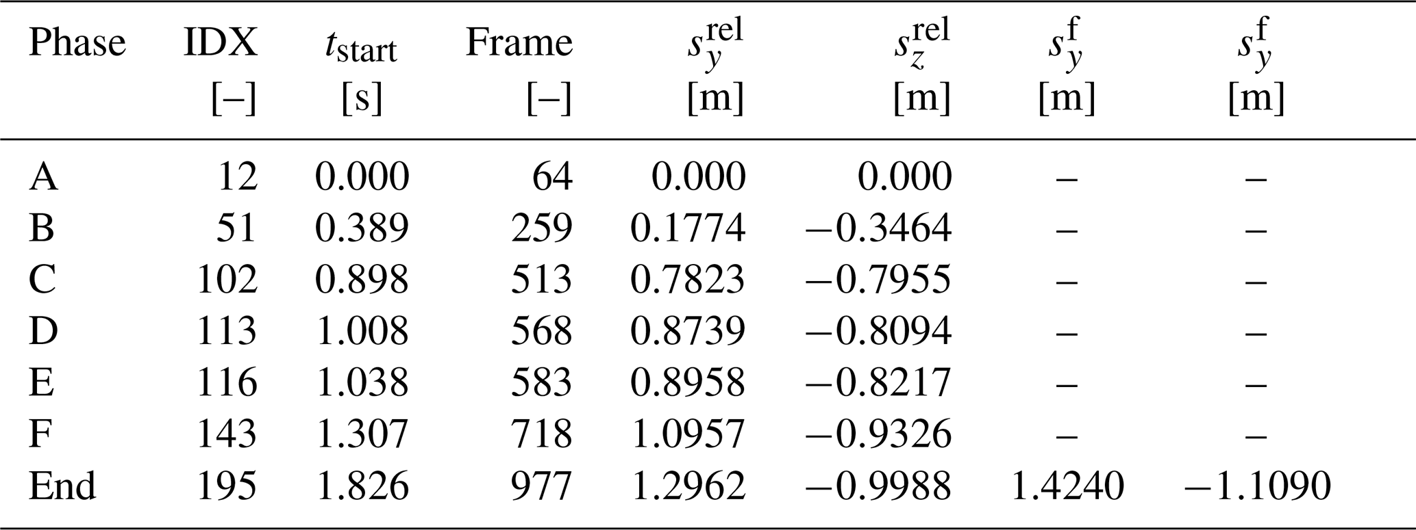
Table 2Motion phases of pebble 4 as displayed in Figs. 3–5 and high-speed video. IDX gives the index of data samples, and tStart gives the time in seconds since the start of motion. Frame is indicated by the frame number as displayed in Video 1. For other columns see description within the text.
Relatively low acceleration values are calculated during phase A. As displayed in Fig. 4a, generally increases until at approx. 0.32 s a local maximum of approx. −9.4 m s−2 occurs. This is less than gravitational acceleration (9.81 m s−2). Therefore, it can be reasoned that free-fall conditions were not totally developed during this phase. In fact, pebble 4 was confined by the underlying mass. This can also be seen in Fig. 4d, where pebble 4 “swims” at the surface of the moving material. Therefore, phase A could be termed as “confined fall”. The highest derived velocity of during phase A was calculated at approx. 1.7 m s−1 at 0.379 s. Afterwards the velocity component decreased. Simultaneously, the velocity component increased further. During phase A, a cumulated vertical distance of approx. 0.35 m was covered. The component amounts to approx. 0.18 m at the end of phase A (see Table 2).
At 0.389 s after the start, a discontinuity on the x and z axes is visible in Fig. 4a and b. The corresponding capture of the high-speed sequence is shown in Fig. 4d. The variability of the acceleration time series increases. This was already identified in Fig. 3. A first strong peak of approx. 14.7 m s−2 occurred at and marks the beginning of phase B. At this time, a transition from confined fall to translational movement occurs. Additionally, the peaky pattern of the acceleration and velocity curves indicates pronounced clast contact and energy dissipation. This is particularly clear for . Because pebble 4 moves at the surface of the material, clast contact occurs mainly in the vertical direction. During phase B, the vertical velocity component subsequently decreases. Meanwhile, increases until at 0.609 s the maximum of approx. 1.45 m s−1 is reached.
Phase C again is introduced by a sudden strong increase in at 0.898 s (diamond II). The acceleration peak at 0.908 s of approx. 35.9 m s−2 leads to a positive vertical velocity of approx. 0.21 m s−1. The pebble consequently moves upwards at this point in time, which can be seen in the displacement plot (Fig. 4c). Afterwards, the displacement tends again to downward motion in phases D and E. During phases C to E, the displacement plot (Fig. 4c) shows stair-like features at the and curves. These features can only be achieved if the actual motion acts against the tendency of downward movement parallel to the flume bottom (see Fig. 1). Together with the previously mentioned high ω around all probe axes (compare Fig. 3), a complex rotational-motion pattern can be interpreted until 1.307 s. Note that only the first milliseconds of this complex motion are visible in Video 1, since pebble 4 left the field of view at approx. 1.0 s.
In phase F, the components of translational acceleration and derived velocity gradually decline, which leads to only little displacements. A total displacement of approx. 1.0 m in the zrel direction and 1.3 m in the yrel direction was calculated by means of the formerly mentioned algorithm. Additionally, in Fig. 4c the covered distance measured with a laser distance meter in the flume direction is plotted. Although being aware that yrel and yf do not necessarily have to be identical (compare Fig. 1 and Sect. 2.2), a high agreement between sensor-derived and manually measured displacements is displayed. It can be reasoned that the probe must be oriented more or less in the flume direction, following that the probe axes xrel and yrel approximate xf and yf. As the vertical direction is derived from ACC readings under stationary conditions, zrel equals zf. Thus, the deviation between and reflects the quality of the sensor-derived position. Whereas a sensor-derived vertical displacement of 0.999 m was calculated, a true vertical displacement of 1.109 m was measured in fact (see Table 2). This means the calculations underestimate the vertical displacement by less than 10 %.
3.3 Visualizing motion by trajectory reconstructions
As described in Sect. 1, high-speed video recording is one of the traditional methods to observe rapid movements. Such a video sequence was recorded for the present study as well (Video 1). Due to narrow conditions at the experimental facility, the high-speed camera had to be installed very close to the setup, resulting in a relatively small field of view. At the end of the high-speed sequence, nevertheless the start of a complex rotational motion of pebble 4 can be observed. However, the full motion feature is not visible.
Although only the first portion of this complex motion is visible on the high-speed sequence, the full trajectory can be reconstructed by means of the recorded Smartstone data. The trajectory is defined as the position vector composed of , and for each time step (Fig. 4c). As additional information, the pebble’s orientation can be reconstructed by means of the previously described algorithm. Consequently, these variables can be plotted as a function of time within a Cartesian coordinate system, as displayed in Fig. 5. Thereby, the axes xrel, yrel and zrel denote the distance axes relative to the starting position of the pebble. Note that zrel always points in the vertical direction (for explanation see above) and that diagram axes of Fig. 5 are not drawn to the same scale. Note further that contrary to Figs. 3 and 4, Fig. 5 shows no time series but visualizes the pebble’s position within the relative reference system.
In Fig. 5a, the trajectory projected on the yrelzrel plane can be seen, displayed in the same orientation as in Video 1. Additionally to the side view perspective, data can also be visualized from a top view, where the trajectory is projected on the xrelyrel plane (Fig. 5b). Moreover, the 3D trajectory can be visualized as displayed in Fig. 5c. The pebble's position is marked by small black dots, and the probe’s axes are shown in red (xp), green (yp) and blue (zp), indicating its orientation at each position. Note that the axes are smaller if they point towards the viewer or the opposite (off the displayed plane). Positions (black dots) are plotted with a constant frequency, which was reduced to of the recording frequency of 100 Hz, for reasons of clarity.
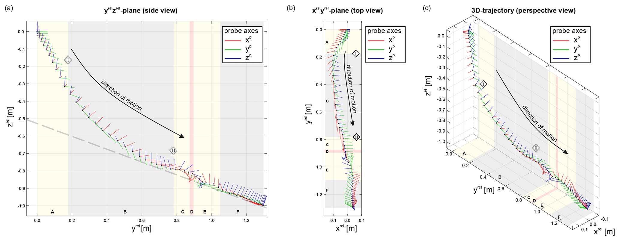
Figure 5Visualization of the reconstructed trajectory within the relative reference system. Red, green and blue coloured lines indicate probe axes and display its orientation within the relative reference system as defined in Sect. 2.2. Motion phases and distinct time points are indicated as in Fig. 3. (a) 2D side view (yrelzrel plane), (b) 2D top view (xrelyrel plane) and (c) 3D perspective view. The dashed grey line represents the tilted flume for illustration.
On the side view plot (Fig. 5a), yp and zp are almost drawn in full length, whereas xp is short, indicating its orientation towards the viewer's perspective. It can be reasoned that the pebble is oriented almost horizontally before the motion begins. By comparing the three plots of Fig. 5, one can observe that the probe is slightly tilted around the yp axis towards the left side.
During phase A, mainly vertical displacement can be seen in Fig. 5a. Projected on the yrelzrel plane, the trajectory shows an almost linear pattern. On the xrelyrel plane (Fig. 5b), a slight rightward displacement is visible. The pebble's orientation remains more or less constant, and only minor tilting can be observed as the yp axis (green) points a little downwards. At the end of phase A, the pebble rotates back again.
In phase B, a transition to a curved trajectory can be observed in Fig. 5a. Interestingly, a major change in the movement direction emerges on the top view at diamond I as well (Fig. 5b). Whereas the pebble moves slightly to the left during phase A, a change in the movement direction towards the right is induced at this point in time. Additionally, a slow rotation of the pebble can be observed in phase B mainly around the yp axis. This rotation contains portions around the other axes as well. Note also that from the beginning of phase A to about the middle of phase B (approx. 0.5 m on yrel), the distance between the small black dots (indicating its position) increases, indicating increasing velocity given a constant rate of displaying the position (33.3 Hz, see above). Afterwards, the distance between the position points decreases, resulting from the deceleration of the pebble.
At diamond II, a major transition was identified above for both probe data and movement characteristics. The same transition is obvious in Fig. 5 as well. While axis configurations only varied slightly during phases A and B, pronounced changes can be seen during phases C to E. The whole complexity of the rotation in these phases can be recognized by comparing the three plots of Fig. 5. It is visible that the pebble rotates around all axes. Further, the distances between single black dots increases again, implying repeated acceleration. Although these rotations were not completely documented by the high-speed sequence (Video 1), the reconstructed 2D and 3D trajectories reveal the complex rotation that was induced by a sudden impact at diamond II (compare also Figs. 3 and 4).
Phase F is again characterized by relatively small but continuous changes in axes orientations and by an almost linear trajectory pattern. The distances between the black dots decrease further, reflecting the decreasing velocity. In addition, Fig. 5 shows that the pebble's orientation at the end of motion differs significantly from its starting orientation. The pebble is strongly rotated as the xp and yp axes point towards the starting position. This could not be identified in the probe data plotted in Fig. 3. Here, only little changes in ACC readings were identifiable. This reflects critical states, where different orientations lead to similar (or equal) axis readings. To derive the correct orientation, advanced techniques have to be used, like a quaternion-based approach (compare e.g. Hanson, 2006). Apart from that, the zp axis points – slightly tilted – in an upward direction. Note also that the flume bottom is inclined by 20∘ (compare Fig. 2). Therefore, the linear trajectory reflects parallel motion along the flume bottom.
4.1 Trajectories of multiple pebbles in one experiment
A detailed analysis of the reconstructed motion behaviour of a single clast within a moving mass was given above. Beyond that, three more pebbles were equipped with Smartstone probes in the same experiment, and their trajectories could be reconstructed in the same way as for pebble 4. Consequently, the four trajectories can be plotted together within one diagram providing that a higher-ordered reference system is applied (see Sect. 2.2 and Fig. 1).
Figure 6 shows the reconstructed spatiotemporal trajectories of four pebbles that were equipped with a probe. Note that vertical and horizontal axes of the diagram are drawn on same scale, and the duration is colour-coded relative to the start of movement. Additionally, time stamps are displayed at 0.25, 0.5, 1.0 and 1.5 s for each trajectory, respectively. The first motion of the four analysed pebbles was set to 0.0 s (pebble 1). Therefore, both time and position coordinates differ from Figs. 3 and 5. Thick grey lines give the dimensions of the flume construction including the storage box with the simplified material body prior to the start. It is visible that pebble 1 and 2 were embedded into the material, whereas pebble 3 and 4 were placed at the surface of the material (see Fig. 2).
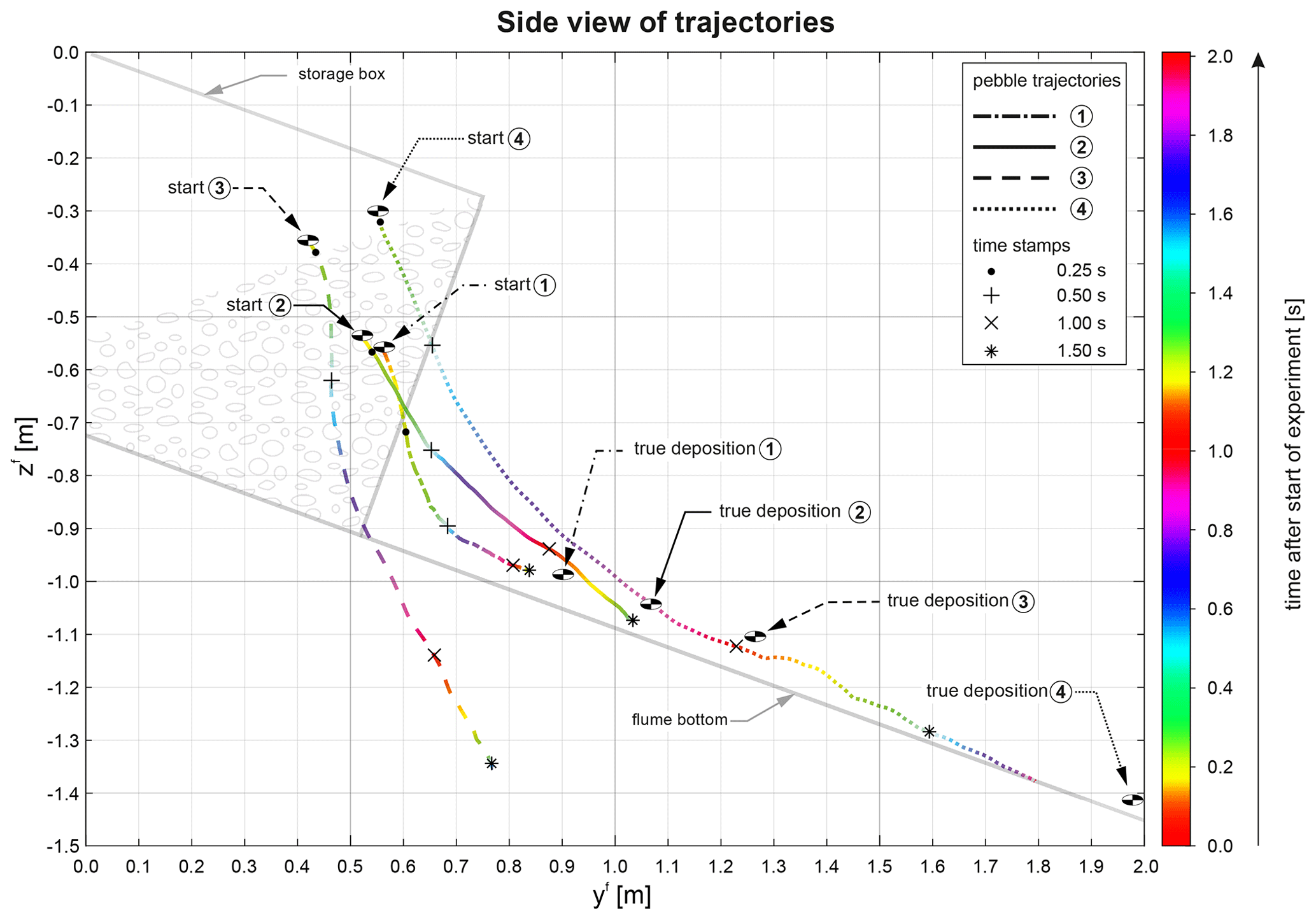
Figure 6Reconstructed spatiotemporal trajectories and true depositional positions of four pebbles within the local flume reference system. 2D side view (yrelzrel plane). In addition, the idealized flume construction and the pebble material body prior to the experiment are drawn in light-grey colours. Note that the equipped pebbles are not drawn to scale due to clearness reasons. The trajectories are colour-coded, where the colour represents the relative time since the start of the experiment (first motion, pebble 1). Additionally, specific points in time are highlighted by time stamps.
Looking at the four trajectories, it can be seen that the path of pebble 3 falls remarkably steeper than the others. This results in a reconstructed depositional position that is below the flume bottom. Here, the reconstruction obviously produces erroneous results. Comparing the end of the trajectory and the true deposition of pebble 3, the overall length (projected length of the 2D displacement on yfzf plane) fits quite well to the measured one. It seems that only the inclination of the reconstructed trajectory was wrongly estimated by the algorithm. A wrong estimation of the initial orientation is considered to be the main disturbance for the wrong orientation of the trajectory. A false reconstruction might occur if the probe did not record the stationary conditions prior to the start of motion. However, the time series of pebble 3 was found to be complete after a detailed review. Another reason could be that – contrary to the other clasts – pebble 3 might be strongly inclined under stationary conditions prior to the start of the experiment. This would result in a wrong estimation of the vertical direction leading to an overestimation of the vertical-acceleration component and the double-integrated vertical displacement.
The other trajectories on the other hand show patterns that are reasonable compared to the reference measurements: the two embedded pebbles covered a shorter distance than the pebble placed at the surface. Additionally, at the same point in time – for instance at approx. 1.0 s since the start of the experiment (again red coloured) – pebble 4 has travelled approx. 0.4 m further than the embedded ones. Whereas Okura et al. (2000) observed that blocks positioned at the front were also deposited in the distal zone, the top pebbles travelled the longest distance in our experiment. Regarding the high-speed video, the explanation is given by the tilted gate: the pebbles positioned on the top start their movement both downwards and to the right (from the camera perspective), thus not transferring energy to material formerly placed underneath in the storage box. The higher the pebbles are placed, the bigger their overhang is, resulting in less material vertically underneath. Compared to the uniform initiation (multiple blocks slid coherently) of the motion in Okura et al. (2000), less energy dissipation occurs in our experiment.
Moreover, the embedded pebble 1 displaced roughly 70 % of the resulting distance (approx. 0.35 m of 0.50 m) within approx. 0.5 s (light-blue colours). It is conspicuous that during this phase mainly vertical displacement occurs, whereas for the latter 30 % of its trajectory it moves more or less parallel to the inclined flume plane. For this part of its trajectory the pebble needs another approx. 0.8 s until it finally deposits. It can be reasoned that a strong gradient in velocity magnitude after the transition from mainly vertical to lateral displacement occurs. This motion behaviour was only observed for pebble 1 in this experiment. Contrary to pebble 1, the trajectory of pebble 2, which was embedded as well, shows a uniform pattern. In addition, a smooth velocity gradient can be observed, indicated by gradually changing colours. Therefore, the two pebbles, which were embedded at opposite sides of the material (compare Fig. 2), show dissimilar motion patterns. Probably the motion behaviour depends on the pebble's distance to the opening board of the flume. Clasts that are further to it – such as pebble 2 – are surrounded by more material confining a free motion. Therefore, almost free-fall conditions will be easier to achieve closer to the opening as in the case of pebble 1. This is also in agreement with the reconstructed trajectory of pebble 4 that shows a similar pattern until approx. 1 s after the start.
Contrary to the uniform trajectories of pebbles 1 and 2, saltation can be recognized approx. 1.15 s after the start between approx. 1.3 and 1.6 m horizontal distance (yf) for pebble 4. This feature is the result of the complex rotations that were identified in probe data (Fig. 3) as well as the derived movement characteristics (Fig. 4) and were finally visualized in Fig. 5. Now, comparing all valid trajectories within the flume reference system, this bumping pattern of pebble 4 becomes very notable. During this phase the general lateral motion along the inclining plane – driven by gravitational acceleration and decelerated by friction – is interrupted. In fact, the pebble moves more or less horizontally before it falls again and proceeds its “normal” motion. This extraordinary motion pattern was initiated by a strong hit visible in the probe motion data (Fig. 3a) at diamond II. Although the trigger can be identified in the probe data, its actual meaning and, subsequently, a suitable interpretation is only possible if the movement is visualized within the correct spatiotemporal context. Hence, a rudimentary plotting of probe data is not sufficient to describe and interpret geomorphic movement processes adequately.
4.2 Probe restrictions and analytical limitations
The current Smartstone probe v2.0 exhibits one main drawback. Since the probe development focussed on the minimal possible size, only a small button cell battery can be used as its energy supply. This means that battery life is restricted, especially under cold conditions. This resulted in pronounced battery wastage. During the future development of the Smartstone probe, alternative options for energy supply will have to be evaluated.
Beyond the battery issues, some probes seemed to be error-prone. As indicated before, it was not possible to record a calibration sequence with one probe. Although this probe was handled in the same way as all others, it was somehow damaged. In this case, an initiation of the recording mode was not possible anymore. The reason for this could not be evaluated.
Despite this, all other probes could be used during the experiments, and the data could be used to reconstruct the 3D trajectories as described above. When comparing the end of each valid trajectory and the true depositional position, a particular deviation of several centimetres is visible. In all cases the reconstructed trajectory is shorter than the actual distance that was covered by the pebble. It can be reasoned that the displacement is generally underestimated by the calculations. This is in contrast to the analytical results of Gronz et al. (2016), where mainly the clipping of ACC readings led to an overestimation of the displacement. In the present experiment, clipping was not observed due to the enhancement of the ACC recording range.
Another explanation for an erroneous displacement derivation might be an incorrect duration of the non-stationary period. During data analysis, the beginning and end of the non-stationary period were set manually, since the primary filter approach of x-io Technologies (2013) was not applicable for these kinds of motion processes. As described before, the algorithm was originally developed to track the human gait that is characterized by uniform and distinct motion patterns. Since the motion behaviour of clasts within a moving granular material possesses a higher level of complexity and is less predictable, the necessary filter parameter settings change significantly for each recorded motion. Consequently, for each pebble and in each experiment, multiple filter parameters would have to be found. Therefore, a manual setting was considered to be more effective. Since the start of the motion process is clearly visible in the sensor data (compare Fig. 3), the beginning of the non-stationary period can be set easily. On the other hand, the motion process mostly declines gradually and slowly (compare Sect. 3.1 and 3.2). Therefore, the end of motion was difficult to identify. In a consistent way, the end of non-stationary periods was set to a time step, where almost no rotation was recorded by the GYR. Around this time at the end of the recorded sequences, ACC readings were low as well. This indicates that more or less only gravitational acceleration was acting on the pebble, and acceleration due to transport motion was negligible. Therefore, it is unlikely that a further transport of the pebble and, consequently, an unrecognized displacement occur. Accordingly, somewhat shorter or longer durations at low acceleration magnitudes do not significantly influence the derivation of displacement. Although the manual definition of the end of motion will always be debatable, the effect of a slightly longer or shorter motion is considered to be extremely small.
Other explanations for the deviation between true and calculated distances are (i) errors due to integration and (ii) imprecise estimations of the probe's orientations. Besides others, these errors were discussed in detail by Gronz et al. (2016). Because the probe data have a finite sampling rate and resolution is integrated twice in each time step, a deviation will always occur and will increase with both time and covered distance.
In the present study, the deviation is considered to be mainly caused by imprecise orientation estimations. As deducted by Gronz et al. (2016), an orientation error of only 1∘ will lead to an erogenous displacement of approx. 0.34 m after 2 s of motion. Compared to the former experiments of Gronz et al. (2016), MAG data were not recorded and could therefore not be included into the sensor fusion analysis. Keeping this in mind, a deviation between true and reconstructed displacement of approx. 10 % (pebble 4, see Sect. 3.2) demonstrates a good quality of the applied methodology. Especially the avoidance of clipping errors contributes to this promising result. This was achieved by enhancing the ACC measuring range from ±4 to ±16 g (compare Gronz et al., 2016).
4.3 Possible ways to enhance the probe accuracy
A comparable low deviation was achieved by merging only ACC and GYR data. Therefore, it can be reasoned that a further enhancement would be possible with the inclusion of MAG data. This would also allow for displaying the trajectory in a global reference system. The effect of these enhancements will be within the scope of further studies.
A further accuracy enhancement of the trajectory reconstructions could be achieved by applying methods that are well-established in different disciplines like pedestrian navigation or mobile robotics, like Kalman filtering or Markov localization. The latter approach uses a probabilistic description of the possible position of the pebble as a density field, which is updated in the upcoming time step(s) (Fox et al., 1999). Not only probe data but also information about the surrounding relief (flume geometry) could be used, for instance. Additionally, information about the pebble (e.g. geometry and specific unit weight) or the surrounding material could be implemented. Further studies will have to evaluate which of these pieces of information will lead to an even better reconstruction of the trajectory. Another aspect worth mentioning might be the automatic indication of the motion mode like that proposed by Becker et al. (2015).
4.4 Scaling
A scaling of the recording ranges will be necessary if the Smartstone method is adapted to other experimental scales or velocities. Additionally, the scaling of temporal persistence of movements has to be respected, as the Nyquist frequency to observe the motion without undersampling changes with the rate of movement changes (Yang et al., 2009). This means that a small pebble in a fast-moving landslide will show more abrupt changes in its velocity, trajectory and mode than a large block in a slow landslide. Thus, the ranges of the sensors and the sampling frequency have to be adjusted depending on the landslide velocity and the particle size. Several aspects concerning the sensor recording range for different experimental applications have to be considered.
-
Acceleration range. The expected acceleration depends on the velocity of the landslide, as the strongest peaks occur during non-elastic collisions of moving particles with stationary boundaries, e.g. bedrock. Thus, the range needs to be increased (by choosing a different accelerometer chip in the Smartstone) with velocity. However, to choose a gratuitously large range to avoid clipping is counterproductive, as the quantization error will also increase because there is only a limited number of steps within the range. A deliberated balance needs to be chosen, e.g. by performing preliminary tests.
-
Gyroscope range. The rotational velocity depends not only on the movement of the landslide but also on the size of particles. For instance, if the mass moves at 1 m s−1, a single rolling pebble with a 30 mm diameter will show a rotational velocity of 3820∘ s−1 (pebble circumference of 942 mm, thus 10.6 rotations per second). Thus, the expected range can be calculated using the shortest circumference of the host particle of the Smartstone(s) and the expected landslide velocity. Again, choosing a gratuitously large range to avoid clipping will increase the quantization error.
4.5 Potentials of the Smartstone probe
Although the exact depositional position could not be reconstructed quantitatively, which is particularly pronounced for pebble 4, qualitative depositional features were found correctly. For instance, pebbles 1 and 2 were embedded before and were also within the deposit after the experiment. This can be concluded from the relatively large vertical distance between the end of trajectory and the flume plane. Contrary to that, pebble 4 was originally deposed directly at the inclined plane which is also reproduced by means of probe data.
Furthermore, the complex rotational movement of pebble 4 can be identified in the reconstructed 3D trajectory. This particular feature becomes also clear if one compares the trajectory of pebble 4 with the other reconstructed transport paths (see above and Fig. 6). Contrary to pebble 4, the other clasts follow relatively simple trajectories. This can be explained by the position of these clasts embedded within the body. Therefore, the motion was strongly confined. Although only data of four probes could be analysed, prominent differences of the motion behaviour dependent on different positions within the moving mass could be found.
These results demonstrate the potential of using in situ motion sensors to characterize artificial landslide movements. Contrary to external-observation methods, such as high-speed videos or laser techniques (e.g. Manzella and Labiouse, 2009), the internal measurement supplies continuous movement characteristics for a single particle in 3D space. The Smartstone probe thereby overcomes the issue of confining the motion process by wires. This problem emerged in many experimental studies that tried to measure the internal deformation or movement characteristics (e.g. Moriwaki et al., 2004; Ochiai et al., 2004, 2007; Olinde and Johnson, 2015). Although the influence due to wired sensors seems small, its exact effect on the motion process cannot be determined. By means of unwired sensors this methodological inaccuracy can be avoided.
In the future, Smartstone probes may help to explain observations from the modelling of landslide motion processes. For instance, it would be interesting to investigate the influence of clasts with different sizes. Phillips et al. (2006) observed a uniform distribution of fine and coarse particles in laboratory high-mobility granular flows. Providing the right scale (compare Sect. 4.4), trajectory reconstruction of different clasts may shed light on the question about how different clast sizes segregate during the transport process. A deeper analysis of the probe data may also allow for estimations of energy dissipation within the landslide body during the motion process (compare e.g. Manzella and Labiouse, 2013).
Beyond these geoscientific objectives, the Smartstone probe was successfully used in experiments focussing on coastal-engineering and hydro-engineering problems. Santos et al. (2019) briefly reported experiments to investigate the stability of breakwater amour units. By means of the Smartstone probe data, Ravindra et al. (2020) presented a detailed analysis of the failure mechanism of placed riprap on laboratory dam models. These examples demonstrate the broad applicability of the Smartstone technique.
During the last years, both wired and unwired sensors (IMU or other combinations of ACC, GYR and MAG) were used to observe geomorphic-motion transport processes. Ooi et al. (2014, 2016) for instance used it to study the initiation process of small-scale laboratory landslides. They used the ACC data for qualitative interpretations concerning the timing of landslide initiation. Additionally, they interpreted a rotational failure process from changing vectorial portions of the gravity vector on different axes. Nevertheless, a quantitative characterization was not carried out. The potential of recording motion data of geomorphic movements is far beyond a simple plotting of probe data. In fact, it allows for the sampling of movement characteristics. Therefore, the recording and analysis of geomorphic-motion data expand the toolkit of landslide science.
Recently, Spreitzer et al. (2019) used an approach similar to that in the present study to derive Euler angles of moving wood in laboratory experiences. They illustrate the suitability of this technique to characterize certain transport features. Beyond the derivation of Euler angles, the present study demonstrates that the calculation of movement characteristics and the reconstruction of spatiotemporal trajectories are essential to describe geomorphic-motion processes adequately.
These derivations are possible even if only acceleration and rotation data are recorded by means of a 6-DoF (degrees of freedom) probe. Further, a full 3D reconstruction of multiple trajectories was achieved. This allows for a comparison between different parts of the moving mass. Accordingly, the present study demonstrates that the “sampling of motion”of single stone movements is possible.
Laboratory experiments are a common tool to study landslide processes in detail. However, a critical – but also difficult – task is to capture the internal dynamics of the moving material. In the present paper, we presented the autonomous Smartstone probe v2.0 that is able to measure in situ motion data of single clasts moving embedded or superficially in/on a landslide mass. The main conclusions of the present study can be summarized as follows:
-
The Smartstone probe in its recent version fulfils all requirements to use it as an additional tool to capture single clast movements in laboratory-scale artificial landslides. Especially its size and measuring range satisfy the development aims. Additionally, the probe dimensions are adaptable to other experimental conditions or research objectives. The Smartstone probe can be used under dry and wet conditions and is able to move, record and transmit data autonomously and wirelessly. The communication works under low-power conditions via active RFID (contrary to the high-power conditions of WLAN).
-
Already the calibrated probe data offer broad insights into the motion process. By means of the acceleration and rotation time series the motion sequence of pebble 4 could be subdivided into six phases with individual motion behaviour. A qualitative interpretation of the probe data reveal stationary, (almost) zero-g, translational and rotational-motion modes. Moreover, a complex rotational motion could be identified, which is initiated by strong acceleration peaks and characterized by angular velocities.
-
Using sensor fusion algorithms, the motion sequence can be quantified within a local reference system. Quantifying motion requires a calculation of the movement characteristics (arel, vrel and srel). This could be achieved satisfactorily by merging acceleration and rotation data. Sensor fusion allows for the in situ measurement of movement characteristics independently from visual contact with the object of interest and without confining wires. Therefore, smart-sensor technology provides the opportunity to sample movement characteristics directly within a moving mass of individual clasts.
-
By means of the calculated movement characteristics, a full 3D reconstruction of the trajectory was possible. This is a great tool to visualize motion and facilitates the qualitative interpretation of transport processes.
-
Finally, it was demonstrated that multiple Smartstone probes can be applied in one experiment. Using this metaphor, this allows for taking multiple motion samples from different parts of a moving landslide body. This opportunity may shed light on the internal dynamics and potential deformation of moving landslide bodies.
Although the Smartstone probe prototype has to be further improved (see Sect. 4.2), the present study indicates a methodological enhancement by means of smart sensors and sensor fusion algorithms. The present study also demonstrates the potentials of cooperation between private enterprise companies and research institutes. The Smartstone probe was developed and manufactured in cooperation with the company Smart Solutions Technology GbR, Germany. Besides the development process, future studies will have to focus on the comparability to other well-established methods, for instance PIV. Beyond that, new analytical solutions have to be found to deal with motion data in geoscience. Therefore, future studies will focus on the question of how motion characteristics like the transport mode can be classified by means of this kind of data.
The data of the four analyzed probes are available on Zenodo: https://doi.org/10.5281/zenodo.4316597 (Dost et al., 2020). The MATLAB code was published by x-io Technologies (2013) under CC license.
A supplementary high-speed video (Video 1) is available online.
The supplement related to this article is available online at: https://doi.org/10.5194/nhess-20-3501-2020-supplement.
BD planned and carried out the present study. He prepared and conducted the experiments; analysed, visualized and interpreted the data; and wrote the present article. OG developed key parts of the experimental setup, helped to conduct the experiments, created the high-speed video, interpreted the data and wrote parts of the article. MC was involved in the development process of the Smartstone probe and the experimental setup, supervised the work, interpreted the data, and reviewed the article. AK helped to develop the experimental setup, interpreted the data and reviewed the article.
The authors declare that they have no conflict of interest.
Many thanks to Yannick Hausener for his great work constructing the experimental flume. The authors additionally thank the former students Julius Weimper, Björn Klaes and Christoph Löber for their help conducting the experiments. Sieving analysis was kindly carried out by Grundbaulabor Trier Ingenieurgesellschaft mbH, Germany.
The Luxembourg Institute of Science and Technology partly funded the experimental setup through the framework of the internship of J. Bastian Dost and the Smartstone probe v2.0. The publication was funded by the Open Access Fund of Trier University and the German Research Foundation (DFG) within the Open Access Publishing funding programme.
This paper was edited by Oded Katz and reviewed by two anonymous referees.
Aaron, J. and McDougall, S.: Rock avalanche mobility: The role of path material, Eng. Geol., 257, 105126, https://doi.org/10.1016/j.enggeo.2019.05.003, 2019. a
Becker, K., Gronz, O., Wirtz, S., Seeger, M., Brings, C., Iserloh, T., Casper, M. C., and Ries, J. B.: Characterization of complex pebble movement patterns in channel flow – a laboratory study, Cuadernos de Investigación Geográfica, 41, 63–85, https://doi.org/10.18172/cig.2645, 2015. a
Bosch Sensortec GmbH: BMC150: Data sheet: 6-axis eCompass, available at: https://www.bosch-sensortec.com/bst/products/all_products/bmc150 (last access: 3 March 2019), 2014. a, b
Bosch Sensortec GmbH: BMI160: Data sheet: Small, low power inertial measurement unit, available at: https://www.bosch-sensortec.com/bst/products/all_products/bmi160 (last access: 3 March 2019), 2015. a, b
Cameron, C.: A Wireless Sensor Node for Monitoring the Effects of Fluid Flow on Riverbed Sediment, Project report, University of Glasgow, Glasgow, 2012. a
Davies, T. R. and McSaveney, M. J.: Runout of dry granular avalanches, Can. Geotech. J., 36, 313–320, https://doi.org/10.1139/t98-108, 1999. a
Dost, J. B., Gronz, O., Casper, M. C., and Krein, A.: Smartstone probe data of a landslide experiment, Zenodo, https://doi.org/10.5281/zenodo.4316597, 2020. a
EIDEN: Kenner Betonwerk EIDEN GmbH: Schüttgüter – Preisliste, available at: http://www.kenner-betonwerk.de/de/produkte/schüttgüter, last access: 21 April 2017. a
Ergenzinger, P., Schmidt, K. H., and Busskamp, R.: The pebble transmitter system (PETS): first results of a technique for studying coarse material erosion, transport and deposition, Z. Geomorphol., 33, 503–508, 1989. a
Fox, D., Burgard, W., and Thrun, S.: Markov Localization for Mobile Robots in Dynamic Environments, J. Artific. Intel. Res., 11, 391–427, https://doi.org/10.1613/jair.616, 1999. a
Frosio, I., Pedersini, F., and Borghese, N. A.: Autocalibration of MEMS Accelerometers, IEEE T. Instrum. Meas., 58, 2034–2041, https://doi.org/10.1109/TIM.2008.2006137, 2009. a
Gronz, O., Hiller, P. H., Wirtz, S., Becker, K., Iserloh, T., Seeger, M., Brings, C., Aberle, J., Casper, M. C., and Ries, J. B.: Smartstones: A small 9-axis sensor implanted in stones to track their movements, Catena, 142, 245–251, https://doi.org/10.1016/j.catena.2016.03.030, 2016. a, b, c, d, e, f, g, h
Hanisch, J., Ergenzinger, P., and Bonte, M.: Dumpling – an intelligent boulder for studying internal processes of debris flows, in: Debris-flow hazards mitigation: Mechanics, prediction, and assessment, vol. 2, edited by: Rickenmann, D. and Chen, C. L., Millpress, Rotterdam, the Netherlands, 843–850, 2003. a
Hanson, A. J.: Visualizing quaternions, Morgan Kaufmann series in interactive 3D technology, Morgan Kaufmann, San Francisco, CA, Amsterdam, Boston, 2006. a
Hofland, B., Arefin, S. S., van der Lem, C., and Van Gent, M. R. A.: Smart Rocking Armour Units, in: Proceedings of the 7th International Conference on the Application of Physical Modelling in Coastal and Port Engineering and Science, edited by: Coastlab18, Santander, Cantabria, Spain, 2018. a
Jazar, R. N.: Advanced dynamics: Rigid body, multibody, and aerospace applications, Wiley, Hoboken, NJ, 2011. a
Koch, W.: Tracking and sensor data fusion: Methodological framework and selected applications, Mathematical Engineering, Springer, Berlin, Heidelberg, https://doi.org/10.1007/978-3-642-39271-9, 2014. a
Madgwick, S. O. H., Harrison, A. J. L., and Vaidyanathan, A.: Estimation of IMU and MARG orientation using a gradient descent algorithm, IEEE Int. Conf. Rehabil. Robot., 2011, 5975346, https://doi.org/10.1109/ICORR.2011.5975346, 2011. a, b, c
Manzella, I.: Dry rock avalanche propagation: unconstrained flow experiments with granular materials and blocks at small scale, PhD thesis,École Polytechnique Fédérale de Lausanne, Laussanne, https://doi.org/10.5075/EPFL-THESIS-4032, 2008. a
Manzella, I. and Labiouse, V.: Flow experiments with gravel and blocks at small scale to investigate parameters and mechanisms involved in rock avalanches, Eng. Geol., 109, 146–158, https://doi.org/10.1016/j.enggeo.2008.11.006, 2009. a, b
Manzella, I. and Labiouse, V.: Empirical and analytical analyses of laboratory granular flows to investigate rock avalanche propagation, Landslides, 10, 23–36, https://doi.org/10.1007/s10346-011-0313-5, 2013. a, b
Moriwaki, H., Inokuchi, T., Hattanji, T., Sassa, K., Ochiai, H., and Wang, G.: Failure processes in a full-scale landslide experiment using a rainfall simulator, Landslides, 1, 277–288, https://doi.org/10.1007/s10346-004-0034-0, 2004. a, b
Ochiai, H., Okada, Y., Furuya, G., Okura, Y., Matsui, T., Sammori, T., Terajima, T., and Sassa, K.: A fluidized landslide on a natural slope by artificial rainfall, Landslides, 1, 211–219, https://doi.org/10.1007/s10346-004-0030-4, 2004. a
Ochiai, H., Sammori, T., and Okada, Y.: Landslide Experiments on Artificial and Natural Slopes, in: Progress in Landslide Science, edited by: Sassa, K., Springer, Berlin, 209–226, 2007. a, b
Okura, Y., Kitahara, H., Sammori, T., and Kawanami, A.: The effects of rockfall volume on runout distance, Eng. Geol., 58, 109–124, https://doi.org/10.1016/S0013-7952(00)00049-1, 2000. a, b, c, d
Olinde, L. and Johnson, J. P. L.: Using RFID and accelerometer-embedded tracers to measure probabilities of bed load transport, step lengths, and rest times in a mountain stream, Water Resour. Res., 51, 7572–7589, https://doi.org/10.1002/2014WR016120, 2015. a
Ooi, G. L., Wang, Y.-H., Tan, P. S., So, C. F., Leung, M. L., Li, X., and Lok, K. H.: An Instrumented Flume to Characterize the Initiation Features of Flow Landslides, Geotech. Test. J., 37, 20130158, https://doi.org/10.1520/GTJ20130158, 2014. a, b
Ooi, G. L., Tan, P. S., Lin, M.-L., Wang, K.-L., Zhang, Q., and Wang, Y.-H.: Near real-time landslide monitoring with the smart soil particles, in: The 15th Asian Regional Conference on Soil Mechanics and Geotechnical Engineering, vol. 2 of Japanese Geotechnical Society Special Publication, Japanese Geotechnical Society, Fukuoka, Japan, 1031–1034, https://doi.org/10.3208/jgssp.HKG-05, 2016. a
Phillips, J. C., Hogg, A. J., Kerswell, R. R., and Thomas, N. H.: Enhanced mobility of granular mixtures of fine and coarse particles, Earth Planet. Sc. Lett., 246, 466–480, https://doi.org/10.1016/j.epsl.2006.04.007, 2006. a
Ravindra, G. H., Gronz, O., Dost, J. B., and Sigtryggsdóttir, F. G.: Description of failure mechanism in placed riprap on steep slope with unsupported toe using smartstone probes, Eng. Struct., 221, 111038, https://doi.org/10.1016/j.engstruct.2020.111038, 2020. a
Ried, M. E., Iverson, R. M., Logan, M., LaHusen, R. H. G., Godt, J. W., and Griswold, J. P.: Entrainment of Bed Sediment by Debris Flows: Results from large-scale Experiments, in: Proceedings of the 5th International Conference on Debris-Flow Hazards Mitigation, edited by: Genevois, R., Hamilton, D. L., and Prestininzi, A., Rome, 2011. a
Santos, J. A., Pedro, F., Coimbra, M., Figuero, A., Fortes, C. J. E., Sande, J., Körner, M., Lemos, R., Bornschein, A., Weimper, J., van den Bos, J., Dost, B., Hofland, B., Carvalho, R. F., Alvarellos, A., Peña, E., Pohl, R., Kerpen, N. B., and Reis, M. T.: 3-D Scale Model Study of Wave Run-Up, Overtopping and Damage in a Rubble-Mound Breakwater Subject to Oblique Extreme Wave Conditions, Defect and Diffusion Forum, 396, 32–41, https://doi.org/10.4028/www.scientific.net/DDF.396.32, 2019. a
Schilirò, L., Esposito, C., de Blasio, F. V., and Scarascia Mugnozza, G.: Sediment texture in rock avalanche deposits: insights from field and experimental observations, Landslides, 16, 1629–1643, https://doi.org/10.1007/s10346-019-01210-x, 2019. a
Spazzapan, M., Petrovčič, J., and Mikoš, M.: New Tracer for Monitoring Dynamics of Sediment Transport in Turbulent Flows, Acta Hydrotech., 22, 135–148, 2004. a
Spreitzer, G., Gibson, J., Tang, M., Tunnicliffe, J., and Friedrich, H.: SmartWood: Laboratory experiments for assessing the effectiveness of smart sensors for monitoring large wood movement behaviour, Catena, 182, 104145, https://doi.org/10.1016/j.catena.2019.104145, 2019. a, b
Volkwein, A. and Klette, J.: Semi-automatic determination of rockfall trajectories, Sensors, 14, 18187–18210, https://doi.org/10.3390/s141018187, 2014. a
Wang, Y.-F., Cheng, Q.-G., Lin, Q.-W., Li, K., and Yang, H.-F.: Insights into the kinematics and dynamics of the Luanshibao rock avalanche (Tibetan Plateau, China) based on its complex surface landforms, Geomorphology, 317, 170–183, https://doi.org/10.1016/j.geomorph.2018.05.025, 2018. a
x-io Technologies: Gait tracking with x-IMU, available at: http://x-io.co.uk/gait-tracking-with-x-imu/ (last access: 3 August 2017), 2013. a, b, c, d
Yang, H., Wei, F., Hu, K., Chernomorets, S., Hong, Y., Li, X., and Xie, T.: Measuring the internal velocity of debris flows using impact pressure detecting in the flume experiment, J. Mount. Sci., 8, 109–116, https://doi.org/10.1007/s11629-011-2083-x, 2011. a
Yang, W. Y., Chang, T. G., Somg, I. H., Cho, Y. S., Heo, J., Jeon, W. G., Lee, J. W., and Kim, J. K. (Eds.): Signals and Systems with MATLAB, Springer-Verlag, Berlin, Heidelberg, https://doi.org/10.1007/978-3-540-92954-3, 2009. a
The sign of the reading does not imply an increase or decrease of velocity. A positive value is caused by acceleration along this axis; a negative value is caused by acceleration in the opposite direction. A positive value as well as a negative value might be due to an increase of the pebble's velocity or a decrease – depending on its orientation.
- Abstract
- Introduction
- Material and methods
- Motion data of landslide experiments and how to read them
- Potentials and limitations of the Smartstone probe
- Conclusions and final remarks
- Data availability
- Video supplement
- Author contributions
- Competing interests
- Acknowledgements
- Financial support
- Review statement
- References
- Supplement