Spatiotemporal changes of seismicity rate during earthquakes

Scientists demystify stress changes within tens of days before a mainshock and often utilize its foreshocks as an indicator. Typically, foreshocks are detected near fault zones, which may be due to the distribution of seismometers. This study investigates changes in seismicity far from mainshocks by examining tens of thousands of M≥2 quakes that were monitored by dense seismic arrays for more than 10 years in Taiwan and Japan. The quakes occurred within epicentral distances ranging from 0 to 400 km during a period of 60 d before and after the mainshocks that are utilized to exhibit common behaviors of seismicity in the spatiotemporal domain. The superimposition results show that wide areas exhibit increased seismicity associated with mainshocks occurring more than several times to areas of the fault rupture. The seismicity increase initially concentrates in the fault zones and gradually expands outward to over 50 km away from the epicenters approximately 40 d before the mainshocks. The seismicity increases more rapidly around the fault zones approximately 20 d before the mainshocks. The stressed crust triggers ground vibrations at frequencies varying from $\sim \mathrm{5}\times {\mathrm{10}}^{-\mathrm{4}}$ to $\sim {\mathrm{10}}^{-\mathrm{3}}$ Hz (i.e., variable frequency) along with earthquake-related stress that migrates from exterior areas to approach the fault zones. The variable frequency is determined by the observation of continuous seismic waveforms through the superimposition processes and is further supported by the resonant frequency model. These results suggest that the variable frequency of ground vibrations is a function of areas with increased seismicity leading to earthquakes.

1 Introduction

Numerous studies (Reasenberg, 1999; Scholz, 2002; Vidale et al., 2001; Ellsworth and Beroza, 1995) reported that foreshocks occur near a fault zone and migrate toward the hypocenter of a mainshock before its occurrence. The spatiotemporal evolution of foreshocks is generally considered to be an essential indicator that reveals variations in earthquake-related stress a couple of days before mainshocks. After detecting these variations, scientists installed multiple instruments along both sides of the fault over short distances to monitor the activity of the fault. However, these instruments typically detect small vibrations near the fault zone. Stress accumulates in a local region near a hypocenter, triggering earthquake occurrence that is concluded from the sparse distribution of seismometers.

Bedford et al. (2020) analyzed the GNSS data and observed crustal deformation in a thousand-kilometer-scale area before the great earthquakes in the subduction zones. Chen et al. (2011, 2014, 2020a, b) filtered the crustal displacements before earthquakes using the GNSS data through the Hilbert–Huang transform. The filtered crustal displacements in a hundred(thousand)-kilometer-scale area before the moderate–large (M9 Tohoku-Oki) earthquakes exhibit paralleling azimuths that yield an agreement with the most compressive axes of the forthcoming earthquakes (Chen et al., 2014). On the other hand, Dobrovolsky (1979) estimated the size of the earthquake preparation zone using the numerical simulation method and found that the radius (R) of the zone is proportional to earthquake magnitude (M). In addition, the relationship can be written by using a formula of R=10^0.43M. These results suggest that a stressed area before earthquakes is obviously larger than the rupture of fault zones. However, it is a big challenge to monitor stress changes in a wide area beneath the ground. A simple way to imagine this is if we place a stick on a table and then hold and try to break the stick. The stress we making on the stick can apply to either a limited local region or to both ends of it. Migrations and propagations of the loading force can be detected according to the changes of strain and the occurrence of microcracks. This common sense suggests that the spatiotemporal evolution of earthquake-related stress appearing a couple of days before mainshocks can be recognized if we can trace the occurrence of relatively small quakes in a wide area (Kawamura et al., 2014; Wen and Chen, 2017). Here we take advantage of earthquake catalogs obtained by dense seismic arrays in Taiwan and Japan to expose foreshocks distributed over a wide area instead of a local region.

2 Methodology

The ability to detect relatively small quakes depends on the spatial density and capability of seismometers. Taiwan and Japan are both the most famous high-seismicity areas in the world. Dense seismometers evenly distributed throughout the whole area are beneficial for monitoring the earthquake occurrences close to and far away from fault zones (Chang, 2014). Earthquake catalogs retrieved from Taiwan and Japan were obtained from the Central Weather Bureau (CWB), Taiwan and the Japan Meteorological Agency (JMA). To distinguish dependencies from independent seismicity, the earthquake catalogs are declustered. Therefore, the ZMAP software package for MATLAB (Wiemer, 2001) was utilized to remove and/or omit influence from duplicate events, such as aftershocks. The declustering algorithm used in ZMAP is based on the algorithm developed by Reasenberg (Reasenberg, 1985). We classify clusters by using the standard input parameters (proposed in Reasenberg, 1985, and Uhrhammer, 1986) for the declustering algorithm. The aftershock clusters in a small area and in a short period of time do not conform to the Poisson distribution, which requires removing the aftershocks from the earthquake sequence. Therefore, some parameters can be set as follows: the look-ahead time for un-clustered events is 1 d, and the maximum look-ahead time for clustered events is 10 d. The measure of probability to detect the next event in the earthquake sequence is 0.95. The effective minimum magnitude cut-off for the catalog is given by 1.5, and the interaction radius of dependent events is given by 10 km (van Stiphout et al., 2012). Earthquakes with depth > 30 km were eliminated from the declustered catalogs to understand seismicity changes before mainshocks mainly in the crust.

Before the analytical processes in this study, we assumed that earthquakes with relatively small magnitude can be the cracks and potentially related to the far mainshocks based on the large seismogenic areas (Bedford et al., 2020). The minimum magnitudes of completeness M_c are 2.0 and 0.0 that can be determined by the declustered earthquake catalogs in Taiwan and Japan, respectively (also see Figs. S1–S4 in the Supplement). The earthquakes with M≥2 are selected and utilized in this study for fair comparison of the seismicity changes during earthquakes in Taiwan and Japan. We classified the selected earthquakes via their magnitudes into three groups (i.e., $\mathrm{3}\le M<\mathrm{4}$, $\mathrm{4}\le M<\mathrm{5}$ and $\mathrm{5}\le M<\mathrm{6}$). Note that the classified earthquakes in each group are determined to be the break events (i.e., the mainshocks). In contrast, the other selected earthquakes with magnitudes smaller than the minima of the classified magnitude are determined to be the crack events.

We construct a spatiotemporal distribution of the crack events for each break quake. The spatiotemporal distribution from 0 to 400 km away from the epicenter of the break quake during a period of 60 d before and after the break occurrence is constructed to illustrate the relationship between the crack events and the break quake in the spatial and temporal domain. Note that the spatial and temporal resolutions of the grids of the spatiotemporal distribution are 10 km and 1 d, respectively, based on the declustering parameters in the ZMAP software (Wiemer, 2001). We count the crack events in each spatiotemporal grid according to distance away from the epicenter and the differences in time before and after the occurrence of the break quake.

Figure 1 Spatiotemporal seismic density distributions in Taiwan and Japan. The seismic densities constructed by using the declustered earthquake catalogs of Taiwan and Japan are shown in the left and right panels, respectively. The seismic density reveals changes in seismicity at distances from the epicenters ranging from 0 to 400 km up to 60 d before and after quakes in a particular magnitude group. The superimposed number in each grid is further normalized for a fair comparison by using the total number of quakes and their areas. Notably, the total number of quakes is shown in the title of each diagram.

The superimposition process, a statistical tool utilized in data analysis, is capable of either detecting periodicities within a time sequence or revealing a correlation between more than two data sequences (Chree, 1913). The process is known as the superposed epoch analysis (Adams et al., 2003; Hocke, 2008). In practice, the superimposition is a process to stack numerous datasets that can migrate unique features for a few datasets and enhance common characteristics for the most datasets. The count in each grid of the spatiotemporal distributions for all the break quakes is superimposed as a total one based on the occurrence time and epicentral distance of the break quakes. The total count of the superimposed distribution in each spatiotemporal grid is normalized to seismic density (count per square kilometer) for comparing to the total number of the break quakes and the related spatial area. Moreover, we compute the average values every distance grid using the seismic densities 60 d before and after the quake. The average values are subtracted from the seismic densities, and the obtained differences are divided by the average values in each distance grid to obtain the normalized variation, clarifying changes of the seismic density in the spatiotemporal domain.

3 Analytical results

The earthquakes with magnitude ≥ 2 listed in the declustered catalogs of Taiwan from January 1991 to June 2017 are utilized to construct a spatiotemporal distribution of foreshocks and aftershocks corresponding to the quakes with $\mathrm{3}\le M<\mathrm{4}$. We superimposed all the crack events corresponding to the 15 625 quakes ($\mathrm{3}\le M<\mathrm{4}$). The seismic density is more than 1000 times greater in a hot region at a distance of 10 km away from an epicenter (which is generally considered to be the gestation area of foreshocks) than it is in areas located >200 km from the epicenter (Fig. 1a). The sudden increase in seismic density suggests that earthquake-related stress accumulates mainly around the hot region, triggering many foreshocks a few days before the earthquakes with $\mathrm{3}\le M<\mathrm{4}$. This partial agreement of the numerous recent studies reported that the seismicity migrates toward the fault rupture zone within tens of kilometers from epicenters a couple of days before earthquakes (Kato et al., 2012; Kato and Obara, 2014; Liu et al., 2019). Meanwhile, the events mainly occur 0–1 d after the quakes, which is irrelevant to the smaller distribution 0–1 d before the quakes (also see Fig. 1). The seismic density close to epicenters (Fig. 1) suddenly increases before and gradually decreases after the quakes. The irrelevance and the differences of changes rates with epicentral distance smaller than 20 km before and after the quakes reveal that the increase in seismicity before the quakes is not contributed by the seismicity after due to the analytical processes in this study. In addition, these analytical results of the seismic activity are also in agreement with the studies in Lippiello et al. (2012, 2017, 2019) and de Arcangelis et al. (2016) with regards to distinct methods.

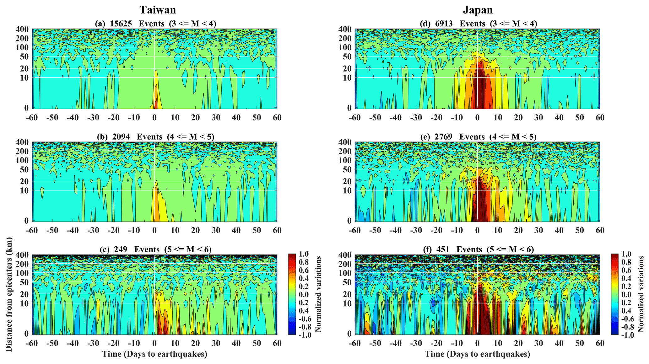
Figure 2 Changes of the normalized spatiotemporal variations in Taiwan and Japan. The normalized variations corresponding to the seismic density in Taiwan and Japan (in Fig. 1) are shown in the left and right panels, respectively. The colors reveal changes of the normalized variations at distances from the epicenters ranging from 0 to 400 km up to 60 d before and after quakes in a particular magnitude group.

On the other hand, the increase in seismic density is not only always limited within the hot region, but also extends outward to a distance of over 50 km away from the epicenters about 0–40 d leading up to the occurrence of the quakes (Fig. 1a). We further examine the spatiotemporal changes in the seismic density up to the M≥4 quakes utilizing the same superimposition process (Fig. 1b and c). The expansion of the increased seismic density about 0–40 d leading up to the occurrence of the quakes and the sharp increases in seismic density a few days before the quakes can be consistently observed using the M≥4 quakes in Fig. 1b and c. Similar results (i.e., the sharp increases in seismic density a few days before the quakes and areas where the increase in the seismicity density is much larger than that of the hot region) can also be obtained using the earthquake catalogs between 2001 and 2010 from the Japan Meteorological Agency (JMA) in Japan (Fig. 1d–f). Note that the earthquakes that occurred on the northern side of the latitude of 32^∘ N were selected from the Japan catalogs. The selection is based on the fact that the earthquakes occurred in the area monitored by the dense seismometer network and to avoid the double count of events in the Taiwan catalogs. The normalized variations corresponding to seismic density in Fig. 1 are shown in Fig. 2. The radii of the positive normalized variations are approximately 50 km while earthquake magnitude increases from 3 to 6 in Taiwan (Fig. 2a–c). The land area of Taiwan is approximately 250 km by 400 km, which causes underestimation of the seismic density in the spatial domain. In contrast, the positive normalized variations roughly expand along the radii ranging from 50 to 150 km, while earthquake magnitude increases from 3 to 6 in Japan (Fig. 2d–f). However, variations in the lead time mostly range from 40 to 20 d, and relationships between the positive normalized variations and the earthquake magnitude can be found in neither Taiwan nor Japan (Fig. 2).

In short, the expansion of the increase in seismic density becomes mitigation and may no longer impact a place at distances > 200 km away from the epicenters for the earthquakes with a magnitude < 6. The increase in seismicity density before the quakes suggests that the accumulation of the earthquake-related stress in the crust originates from the hot region and gradually extends to an external place before earthquakes occur. The area of this external place is several times that of a fault rupture zone that is concluded based on the sparse seismic arrays of the past. If a quake can excite seismicity changes over a wide area (i.e., over 50 km by 50 km), any crustal vibration related to stress accumulation before earthquakes can be too small to be identified from continuous seismic waveforms at one station. In contrast, crustal vibrations can be a common characteristic of continuous seismic waveforms at most stations around fault zones due to the fact that seismicity changes dominated by earthquake-related stress accumulation are distributed in a wide area.

4 The principal component analysis (PCA) on the continuous seismic waveforms

Seismic waveforms obtained from 33 broadband seismometers operated by the National Center for Research on Earthquake Engineering (NCREE) of Taiwan, within a temporal span of approximately 1 year (from June 2015 to June 2016) are utilized in this study. Note that two seismometers of them are eliminated from following the analytical processes due to long data gaps. The principal component analysis (PCA) method (Jolliffe, 2002) is utilized to retrieve the possible stress-related common signals from continuous seismic waveforms on the vertical component at 31 seismic stations over a wide area and to mitigate local noise simultaneously. Figure 3a shows the energy and the cumulative energy of the principal components derived from the continuous seismic waveforms at the 31 stations. The energy of the first principal component is about 12 %, which is more than 3 times that of the following ones. Thus, we determined the first principal component to be the common signals of the ground vibrations before earthquakes. Figure 3b reveals changes in the common signals during the study period along the time. However, no obvious changes can be observed in the temporal domain.

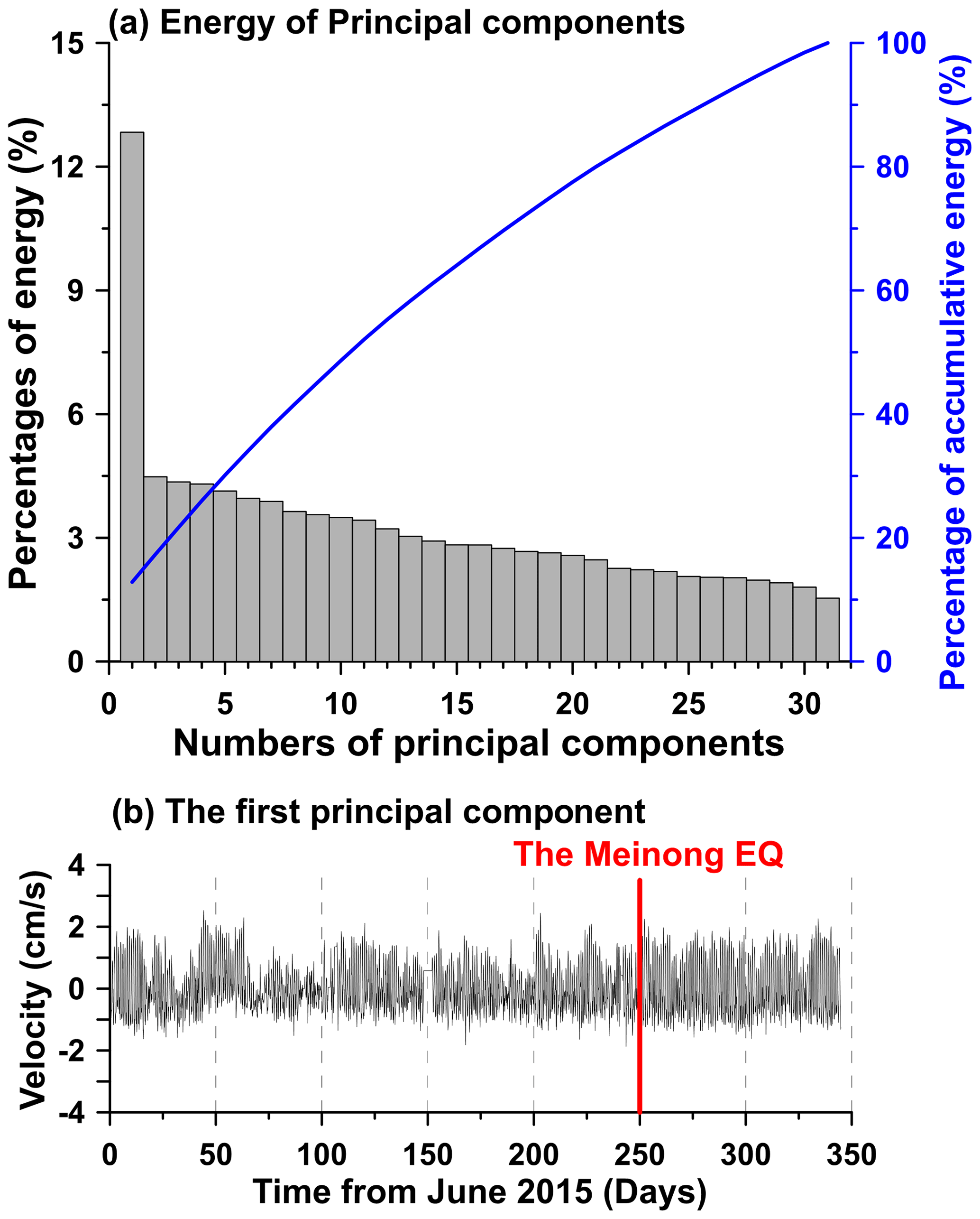
Figure 3 The energy and the first principal component derived from vertical seismic velocity data from the 31 stations. The energy and the cumulative energy of the principal components are shown in (a). Bars denote the energy of each principal component. The blue line shows the variation in the cumulative energy from distinct used principal components. The variations in the first principal component during the period (i.e., from June 2015 to June 2016) are revealed in (b). The red vertical line indicates the occurrence time of the M6.6 Meinong earthquake (on 2 February 2016).

Thus, we sliced the common signals into several time spans using a 5 d moving window with 1 d steps to show time-varying changes. The common signals in each time span are transferred into the frequency domain using the Fourier transform to investigate frequency characteristics of ground vibrations before earthquakes. The amplitudes are normalized using the frequency-dependent average values computed from the amplitude 30 d before and after earthquakes via the temporal division. Here, we take the M6.6 Meinong earthquake (Wen and Chen, 2017; Chen et al., 2020c) as an example to understand the changes of the amplitude of the common signals in the spatiotemporal domain (Fig. 4a). Distinct patterns in the amplitude–frequency distributions can obviously be observed before and after the earthquake at a frequency higher than $\mathrm{5}\times {\mathrm{10}}^{-\mathrm{4}}$ Hz (also see Fig. 4e and f). The amplitude at the frequency close to $\mathrm{5}\times {\mathrm{10}}^{-\mathrm{4}}$ Hz was obviously enhanced approximately 20–40 d before the earthquake. Hereafter, the enhancements were significantly reduced and reached a relatively small value a few days after the earthquake. Meanwhile, the frequency is close to $\mathrm{2}\times {\mathrm{10}}^{-\mathrm{4}}$ Hz approximately 60 d before the earthquake and tends to be high near 10⁻³ Hz a few days before the event (also see Fig. 4e and f). We next superimpose the amplitude based on the occurrence time of the 17 earthquakes with $\mathrm{4}\le M<\mathrm{5}$ and the 109 earthquakes with $\mathrm{3}\le M<\mathrm{4}$ during the 1-year temporal span shown in Fig. 4b and c, respectively. The consistent variations (i.e., the frequency is close to $\mathrm{2}\times {\mathrm{10}}^{-\mathrm{4}}$ Hz approximately some days before the quakes and tends to be high near 10⁻³ Hz a few days before the quakes) can be observed in Fig. 4b and c.

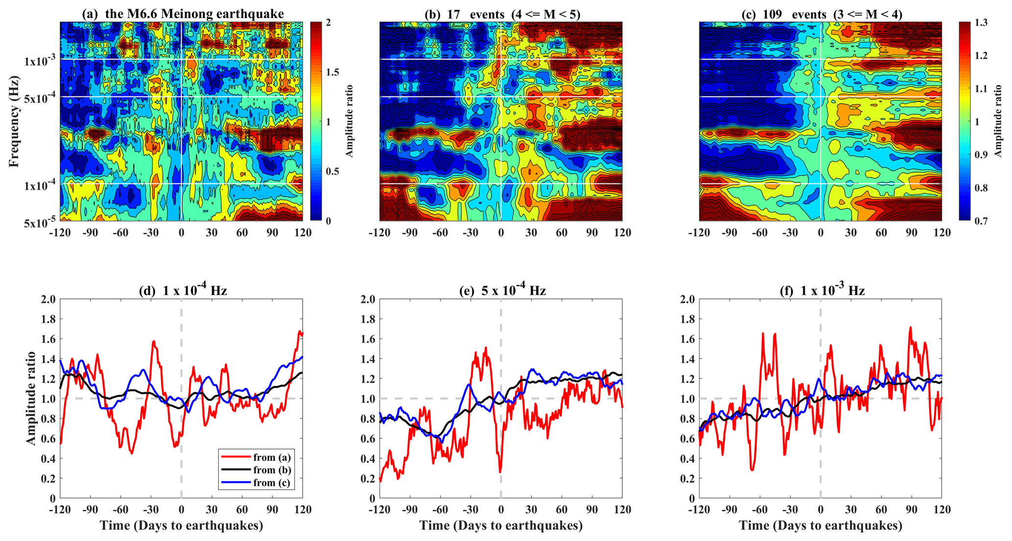
Figure 4 The amplitude ratio of the superimposed time–frequency–amplitude distribution associated with earthquakes with distinct magnitudes. The superimposed results 120 d before and after quakes with the M6.6 Meinong earthquake, $\mathrm{4}\le M<\mathrm{5}$ and $\mathrm{3}\le M<\mathrm{4}$ are shown in (a)–(c), respectively. The distribution is normalized for comparison by using the average amplitude in each frequency band of 30 d before and after the quakes. The total number of earthquakes in each magnitude group is shown in the title of each diagram. Variations in the amplitude ratios in (a)–(c) at frequencies of about $\mathrm{1}\times {\mathrm{10}}^{-\mathrm{4}}$, $\mathrm{5}\times {\mathrm{10}}^{-\mathrm{4}}$ and $\mathrm{1}\times {\mathrm{10}}^{-\mathrm{3}}$ Hz during the same period are shown in (d)–(f), respectively.

Here, we retrieve the ratios at three frequencies of approximately $\mathrm{1}\times {\mathrm{10}}^{-\mathrm{4}}$, $\mathrm{5}\times {\mathrm{10}}^{-\mathrm{4}}$ and $\mathrm{1}\times {\mathrm{10}}^{-\mathrm{3}}$ Hz to reveal the relationship between the enhancements and earthquake magnitudes (Fig. 4d–f). For the Meinong earthquake, the enhancements could be identified at the low frequency of approximately $\mathrm{1}\times {\mathrm{10}}^{-\mathrm{4}}$ Hz. The ratios exhibit a relatively large value of ∼1.2 about 90 d earlier than the earthquake (Fig. 4d). The ratios rapidly decrease to a relatively small value of ∼0.5 near 60 d before the earthquake. The enhancements with the maxima reach ∼1.6 about ∼30 d before the earthquake. After the earthquake, the ratios fluctuate and recover with a relatively large value of ∼1.2 about 100 d after the earthquake. Regarding earthquakes with relatively small magnitude, the enhancements at $\mathrm{1}\times {\mathrm{10}}^{-\mathrm{4}}$ Hz are ∼1.2 for the group of $\mathrm{4}\le M<\mathrm{5}$ and ∼1.1 for the group of $\mathrm{3}\le M<\mathrm{4}$ between 30 and 50 d before the earthquake occurrence (Fig. 4d). Similarly, the enhancements at $\mathrm{5}\times {\mathrm{10}}^{-\mathrm{4}}$ Hz are ∼1.4 for the Meinong earthquake, ∼1.15 for the group of $\mathrm{4}\le M<\mathrm{5}$ and ∼1.05 for the group of $\mathrm{3}\le M<\mathrm{4}$ between 5 and 30 d before the earthquake occurrence (Fig. 4e). The enhancements at $\mathrm{1}\times {\mathrm{10}}^{-\mathrm{3}}$ Hz are ∼1.15 for the Meinong earthquake, ∼1.15 for the group of $\mathrm{4}\le M<\mathrm{5}$ and ∼1.05 for the group of $\mathrm{3}\le M<\mathrm{4}$ between 2 and 30 d before the earthquake occurrence (Fig. 4f). The ratios at the three frequencies in Fig. 4d–f suggest that the amplitude ratios of the enhancements and earthquake magnitudes generally show a proportional relationship. However, the ratios at $\mathrm{1}\times {\mathrm{10}}^{-\mathrm{3}}$ Hz with a relatively large value of ∼1.6 can be observed during the period of 60–45 d before the Meinong earthquake due to unknown disturbances (Fig. 4f).

The findings suggest that the common-mode ground vibrations exist in a wide area before earthquakes due to the signals being retrieved from most stations distributed around all of Taiwan through the PCA method. In short, the common-mode vibrations are very difficult to be identified from the time series data but become significant in the frequency domain. If the expansion of the seismogeneric areas and the existence of the common-mode ground vibrations are true, the next step is to determine the potential mechanism hidden behind this nature.

5 Discussions

Walczak et al. (2017) repeatedly observed stressed rocks exciting long-period vibrations during rock mechanics experiments. Leissa (1969) reported that the resonance frequency of an object is proportional to its Young modulus and exhibits an inverse relationship to its mass. Based on the crust, the outermost of the Earth, being lamellar, we assume that the earthquake-related stress accumulates in the volume of a square sheet with a width of 100 km, which is determined by using a distance of 50 km away from an earthquake due to the significant increase in the seismic density (Figs. 1 and 2). The resonance frequency near $\mathrm{3}\times {\mathrm{10}}^{-\mathrm{4}}$ Hz (Fig. 4) can be derived from the square sheet once the thickness of the volume is ranged between 500 and 1000 m (Fig. S5). Although we do not fully understand the causal mechanism of the thickness, the agreement with the spatiotemporal domain of the relatively small quakes from the earthquake catalogs, the superimposition results of continuous seismic waveforms and the resonance frequency models suggests that the phenomenon of variable frequency may exist tens of days before earthquake occurrence and can be retrieved by broadband seismometers.

In this study, we determined the seismogenic areas using the relatively small earthquakes in the spatiotemporal distribution and found that the areas are significantly larger than the fault rupture zone (Figs. 1 and 2). Meanwhile, the ground vibrations can exhibit frequency-dependent characteristics at about 10⁻⁴ Hz (Fig. 4) that could relate to the large seismogenic areas due to the resonance model (Fig. S5). If these are true, the seismo-TEC (total electron content) anomalies in the ionosphere, which is generally observed in a large-scale area with more than 10 000 km² (Liu et al., 2009), have a high potential to be driven by upward propagation of acoustic waves before earthquakes (Molchanov et al., 1998, 2011; Korepanov et al., 2009; Hayakawa et al., 2010, 2011; Sun et al., 2011; Oyama et al., 2016). The existence of the ground vibrations can generate the acoustic-gravity waves that have been reported (Liu et al., 2016, 2017). However, the acoustic-gravity waves in a period of <300 s are difficult to propagate upward into the atmosphere and the ionosphere (Yeh and Liu, 1974; Azeem et al., 2018). The wide seismogenic areas observed in this study can contribute the larger-scale ground vibrations at approximately $\mathrm{5}\times {\mathrm{10}}^{-\mathrm{4}}$–10⁻³ Hz that cover the frequency channel ($<\mathrm{1}/\mathrm{300}$ Hz) for the acoustic-gravity waves propagating into the atmosphere and changing the TEC in the ionosphere. Meanwhile, the seismo-atmospheric and the seismo-ionospheric anomalies in a large-scale area can also be supported by the acoustic-gravity waves due to the wide seismogenic areas. While partial aforementioned relationships cannot be quickly proven, the ground vibrations at a low frequency ($<\mathrm{1}/\mathrm{300}$ Hz) in a wide area assist our understanding of the essence of the seismo-anomalies in the atmosphere and the ionosphere.

6 Conclusion

The process of stress migration in the spatiotemporal domain can be concluded from tracing the increase in seismicity according to the 10-year earthquake catalogs from dense seismic arrays in Taiwan and Japan. Areas with the increase in seismicity, where stress accumulates in the crust and triggers earthquakes, are seriously underestimated using a sparse seismic array. Seismicity initially increases around hypocenters, and this can be observed more than 50 d before quakes through superimposing large numbers of earthquakes. The seismicity gradually increases along with the expansion of areas from fault zones to an area widely covering an epicentral distance close to 50 km approximately 20–40 d before earthquakes. The crustal resonance exists at a frequency near $\mathrm{5}\times {\mathrm{10}}^{-\mathrm{4}}$ Hz when the expansion becomes insignificant. Instead of the spatial expansion, the sharp increase in seismicity around the hot regions suggests stress accumulation in fault zones generating crustal resonance at a frequency of up to $\sim {\mathrm{10}}^{-\mathrm{3}}$ Hz in the few days before earthquakes. Most broadband seismometers can observe the variable frequency of ground vibrations in Taiwan due to the comprehensive spatial coverage of resonant signals. The variable frequency depends on various stress-dominant areas that can be supported by the potential crustal resonance model. Seismic arrays comprising dense seismometers with a wide coverage are beneficial for monitoring the comprehensive process of stress migration in the spatiotemporal domain leading up to a faraway and forthcoming mainshock.