Forecasting flood hazards in real time: a surrogate model for hydrometeorological events in an Andean watershed

Growing urban development, combined with the influence of El Niño and climate change, has increased the threat of large unprecedented floods induced by extreme precipitation in populated areas near mountain regions of South America. High-fidelity numerical models with physically based formulations can now predict inundations with a substantial level of detail for these regions, incorporating the complex morphology, and copying with insufficient data and the uncertainty posed by the variability of sediment concentrations. These simulations, however, typically have large computational costs, especially if there are multiple scenarios to deal with the uncertainty associated with weather forecast and unknown conditions. In this investigation we develop a surrogate model or meta-model to provide a rapid response flood prediction to extreme hydrometeorological events. Storms are characterized with a small set of parameters, and a high-fidelity model is used to create a database of flood propagation under different conditions. We use kriging to perform an interpolation and regression on the parameter space that characterize real events, efficiently approximating the flow depths in the urban area. This is the first application of a surrogate model in the Andes region. It represents a powerful tool to improve the prediction of flood hazards in real time, employing low computational resources. Thus, future advancements can focus on using and improving these models to develop early warning systems that help decision makers, managers, and city planners in mountain regions.

1 Introduction

Flash floods produced by extreme precipitation events have produced devastating consequences on cities and infrastructure in mountain regions (EEA, 2005; Wilby et al., 2008). In many cases, anthropic factors such as unplanned urban development and climate change can significantly amplify their effects, increasing the risk for the population and affecting their social and economical conditions (Wohl, 2011). The Andes mountain range in South America has been the scenario of many recent floods with catastrophic outcomes (e.g. Houston, 2005; Mena, 2015; Wilcox et al., 2016). The piedmont has also experienced a rapid urban growth, with cities occupying regions near river channels and increasing the exposure of communities and their infrastructure (Castro et al., 2019). In this context, assessing flood hazards and designing strategies to reduce the potential damages caused by flooding are now critical in cities located near mountain rivers. Specifically, implementing efficient and accurate tools that facilitate real-time predictions of potential risks is a key component to provide decision makers with enough time for action and reduce the life-loss potential (Amadio et al., 2003; Resio et al., 2009; Toro et al., 2010; Taflanidis et al., 2013).

One of the main difficulties of predicting flood hazard in real time in these regions comes from the very short time available to provide an accurate estimation of the risk. The complex topography in the Andean foothills is characterized by small watersheds, on the order of 50–1000 km², and very steep slopes that can reach 40^∘. As a consequence, these environments often have very short times of concentration (Amadio et al., 2003), which restricts the option of real-time predictions based on instrumentation along the river network. In this context, numerical models can play a significant role in predicting flood propagation for a set of possible scenarios and understanding their consequences.

Implementing numerical models to simulate flash floods in these regions, however, is far from trivial, since multiple factors oftentimes associated with high levels of uncertainty control the generation and propagation of floods. In Andean regions, particularly, rivers are characterized by complex bathymetries and steep slopes, typical of mountain rivers, that generate propagation of flows with rapid changes of velocity and wet–dry interfaces (Guerra et al., 2014). Large sediment transport, generally produced by hillslope erosion and rilling by the overland flow in areas with steep slopes and low vegetational covering, can play a significant role in the flow hydrodynamics (Contreras and Escauriaza, 2020), altering the momentum balance of the instantaneous flow. Additional factors, such as storms influenced by the South American monsoon (Zhou and Lau, 1998) and El Niño–Southern Oscillation (ENSO), can generate anomalously heavy rainfall (Holton et al., 1989; Díaz and Markgraf, 1992). However, there is a lack of meteorological, fluviometric, and sediment concentration data, used for calibration and validation of models, due to the difficulties of measuring in high-altitude environments, with difficult access, and during episodes of severe weather.

Models can provide accurate results with high resolution in urban areas, incorporating the coupling effect of meteorological, hydrological, hydrodynamics, and sediment transport components. Unfortunately, they might require large computational costs, with hundreds to thousands of CPU hours per simulation (Tanaka et al., 2011), which prevent the timely prediction of flood propagation that is necessary, especially when the uncertainty of the flood conditions requires the evaluation of multiple possible scenarios of a single event (Toro et al., 2010).

Thus, combining physically based high-fidelity models with statistical approaches is a good alternative to provide fast responses, but preserving the high resolution and high accuracy of physically based models. Surrogate models (or also called meta-models) based on interpolation/regression methodologies have already been applied with the same objective for surge predictions during extratropical cyclones (Taflanidis et al., 2013), to substitute hydrodynamic models and predict maximum peak flows during hydrological events (Bermúdez et al., 2018) and estimate flooding maps (Jhong et al., 2017), among others. The general idea consists in (1) developing a database of high-fidelity simulations and (2) parameterizing each storm/simulation through a small number of variables to represent the input for the surrogate model, and the outputs of interest. Then, we (3) provide a fast-to-compute approximation of the input–output relationship. After the surrogate model is developed, it can be used to predict scenarios for new sets of inputs or new storm characteristics that were not simulated with the high-fidelity model.

The objective of our research is to assess the applicability and performance of a surrogate model or meta-model approach, to accurately and efficiently predict flood hazard from hydrometeorological events in an Andean watershed.

We select the Quebrada de Ramón watershed as a study case, which is located in the Andean foothills of central Chile. We develop a set of high-fidelity simulations for a wide range of hydrometeorological scenarios by coupling two models: (1) a semi-distributed hydrological model that transforms precipitation into runoff (Ríos, 2016) and (2) a two-dimensional (2D) high-resolution hydrodynamic model of the non-linear shallow-water equations, which incorporates the effects of high sediment concentrations (Contreras and Escauriaza, 2020). We parameterize the set of high-fidelity simulations by selecting four input parameters that describe the storm events and one output that describes the flood hazard at critical points within the watershed. Then, we implement the surrogate model by statistically interpolating a relationship between inputs and output on the parameter space. In this work, we implement kriging or Gaussian process interpolation, a popular surrogate modeling technique to approximate deterministic data (Couckuyt et al., 2014).

The meta-model can be used to rapidly calculate the flood hazard output for inputs that describe new events. We use physical variables based on the analysis of the results of the high-fidelity model, describing the dynamic interplay between the high sediment concentrations and geomorphic drivers on the flood propagation in mountain streams (Contreras and Escauriaza, 2020), as well as the implementation of the surrogate model. Thus, the surrogate model provides high-resolution results with low computational costs, considerably more inexpensive compared to traditional computational fluid dynamics (CFD) simulations (Couckuyt et al., 2014; Jia et al., 2015), by using a database of precomputed cases for the fast evaluation of multiple scenarios.

The paper is organized as follows: in Sect. 2 we provide a detailed description of the generation of the database that we use to build the surrogate approach, using high-fidelity simulations that combine a hydrological model and a 2D hydrodynamic model for the Quebrada de Ramón stream near Santiago, Chile. In Sect. 3 we describe the statistical interpolation of the surrogate model using kriging. Results for water depth predictions in critical points and flooded areas are described in Sect. 4. In Sect. 5 we provide a discussion of the results, and in the conclusions of Sect. 6 we summarize the findings of this investigation and discuss future research directions.

2 Database generation through high-fidelity simulations

The first requirement to implement a surrogate model is developing a database of high-fidelity simulations that describe the complex interaction between meteorological, hydrological, and hydrodynamic processes during the storms. We select the Quebrada de Ramón watershed, located in central Chile, to the east of the city of Santiago, as our study case. The elevation of the main channel ranges from 3400 to 800 m a.s.l., and the total area of the watershed is 38.5 km². The steep gradients in the basin and channels produce high flow velocities and large sediment concentrations reaching urban areas. The record of flash floods shows that extreme precipitation can be generally accompanied by an increment of temperature and a higher elevation of the 0 ^∘C isotherm, particularly during events affected by the El Niño phenomenon. The flood risk has increased over the last years, since in the lower section of the watershed the natural channel has been replaced with an artificial channel with a design discharge of 20 m³ s⁻¹, i.e., the 10-year flow discharge (Catalán, 2013).

One of the most challenging aspects of modeling this area is the lack of accurate and continuous hydrometeorological data. This is critical at high altitudes, where estimating the location of the 0 ^∘C isotherm is key to predict the total area draining liquid rainfall. The only continuous hydrometeorological data available come from a station located at 527 m a.s.l., at around 10 km west of the outlet of the watershed, which provides daily precipitation and temperature data for approximately 40 years. In terms of streamflow, there is only one gauge at the outlet of the basin, at the critical point in the artificial channel. The gauge has a discontinuous record of monthly, daily, and maximum instantaneous discharge between 1991 and 2015, with gaps especially during extreme weather conditions.

To create the database, we couple hydrological and hydrodynamic models to run 200 years of continuous synthetic precipitation and temperature series, simulating the rainfall–runoff process in the watershed. We use a hydrological model described in Sect. 2.1 to compute the time series of river discharge at the outlet of the natural domain, which corresponds to the entrance to the urban area. Then, we select events such that the maximum instantaneous flow rate exceeds 20 m³ s⁻¹, obtaining a set of 49 different hydrographs. We use the hydrodynamic model of Contreras and Escauriaza (2020), explained briefly in Sect. 2.2, to propagate these hydrographs through the urban area for different sediment concentrations that are quasi-randomly selected within a realistic range for the region. Thus, each simulation in the database describes flow depths and velocities during the flood in the study area, produced by specific hydrometeorological conditions and the high-resolution topography of the terrain.

In the remainder of this section, we provide a detailed description of both the physics-based hydrological and hydrodynamic models and their implementation in the Andean watershed.

2.1 Hydrological model

We develop a continuous rainfall–runoff model using HEC-HMS (Scharffenberg and Fleming, 2010), which transforms meteorological data into discharge hydrographs, based on the work of Ríos (2016). We divide the watershed into subcatchments using a bare-earth digital elevation model (DEM). The model calculates the abstractions for each of the subcatchments (i.e., interception in vegetation, surface storage and infiltration), the evapotranspiration, and the snow melting and accumulation. On the other hand, the base flow and excess runoff are combined to calculate the response hydrograph, which is then propagated to the outlet of the watershed.

Interception by vegetation is calculated using a simple model that considers a maximum storage capacity for each subcatchment, which is a function of the type of vegetation, the season of the year, and the characteristics of the storm (Ponce, 1989). A similar method was used to estimate the surface storage, which depends on the soil properties and the slope (Bennett, 1998). Both the interception and surface storage must be filled before initiating infiltration, which is simulated with the soil moisture accounting (SMA) method (Scharffenberg and Fleming, 2010). The SMA method represents the catchment as a group of different subsurface storage strata, in which infiltration, percolation, the soil humidity dynamics, and evapotranspiration are continuously simulated during wet and dry periods. Evapotranspiration is calculated using the Priestley–Taylor equation (Chow et al., 1988), while snow accumulation and melting are simulated as a function of the atmospheric conditions through the temperature index (Bras, 1990). In the model, the melted snow becomes available on the soil surface and then is added to the rainfall hyetograph (see Scharffenberg and Fleming, 2010, for details).

Base flow in the subcatchments is estimated with a linear reservoir model able to represent an exponential recession curve. The Clark unit hydrograph that propagates the time–land curves through the linear reservoir is used to simulate the direct response of the subcatchment (see Viessman and Lewis, 2003, for details). Because of the low storage and flood attenuation capacity of the channel network in this mountain environment, we use a simple delay method without attenuation to simulate the transit of the hydrographs from every subcatchment to the outlet.

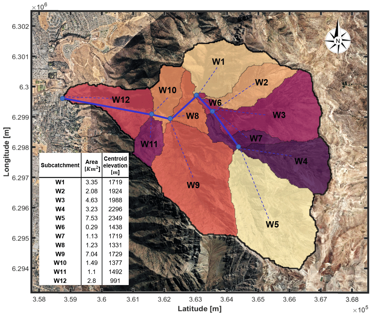
Figure 1 Configuration of the Quebrada de Ramón used in the hydrological model. The colored areas represent each of the subcatchments, enumerated from 1 to 12 in HEC-HMS. The blue lines represent each of the reaches and the blue dots the junctions between them. Background image: © Google Earth.

The Quebrada de Ramón basin was divided into 12 subcatchments whose morphological metrics were obtained from a 2 m resolution bare-earth digital elevation model (DEM), as shown in Fig. 1. We use daily precipitation and temperature data recorded at Quinta Normal station, located at 527 m a.s.l., at around 10 km west of the outlet of the watershed. The data comprise the period from 1 April 1971 to 31 March 2010, which represents 40 hydrological years. To perform the simulation, we used the method proposed by Socolofsky et al. (2001), slightly modified by Ríos (2016), to statistically disaggregate the daily precipitation record to generate 5-hourly synthetic records (i.e., a total of 200 years). These hourly synthetic records in the Quinta Normal gauge were extrapolated to the different subcatchments by considering a linear gradient and the elevations of their centroids. This gradient was estimated using annual precipitation records between 1995 and 2014 for 23 stations located in a surrounded area of 3000 km², whose elevations vary between 176 and 2475 m a.s.l., and was assumed to be unique and constant. Likewise, we extrapolate the records of maximum and minimum daily temperature of Quinta Normal to each subcatchment following the −6.5 ^∘C km⁻¹ gradient, typically used in the zone (Torrealba and Nazarala, 1983; Lundquist and Cayan, 2007). The daily record is disaggregated in an hourly time series, using a procedure based on a Fourier decomposition (Campbell and Norman, 2012). Since there are no series of hourly solar radiation data in the study area, we use the monthly average of solar radiation in the period 2003–2012 for the entire watershed, which is very similar for the region (Ministerio de Energía, 2015).

Due to the lack of a long and reliable record of streamflow data at Quebrada de Ramón, we followed the approach presented in Ríos (2016) to calibrate the model by replicating the most recent annual frequency curve reported in the study area (ARRAU Ingeniería, 2015). We run the model using the 200 years of hourly synthetic record with a time step of 30 min.

In Fig. 2, we compare both the frequency curves of annual maximum discharges. The similarity between both curves demonstrates the ability of the model to simulate large streamflows expected for the basin.

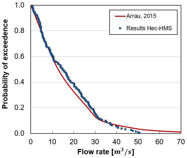
Figure 2 Calibration of HEC-HMS: comparison between measured flow rate and results from the hydrological model.

2.2 Hydrodynamic model

We propagate the floods by solving the non-linear shallow-water equations (NSWEs), which correspond to the conservation of mass and momentum, assuming hydrostatic pressure distribution, negligible vertical velocities, and vertically averaged horizontal velocities. Since the high sediment concentrations can change the rheology of the flow, we modify the equations to account for the heterogeneous density distribution (Contreras and Escauriaza, 2020). We couple the sediment mass conservation equation and include an additional source term in the momentum equations to represent the additional stresses produced by the increase in the density and viscosity of the water–sediment mixture. In the numerical solution, we compute the evolution in time and space of the flow depth h, the volumetric sediment concentration C, and the Cartesian components of the 2D flow u and v in the X and Y directions, respectively.

The equations are solved in non-dimensional form, using a characteristic velocity scale 𝒰, a scale for the water depth ℋ, and a horizontal length scale of the flow ℒ. Two non-dimensional parameters appear in the equations: (1) the relative density between the sediment and water $s={\mathit{\rho }}_{\mathrm{s}}/{\mathit{\rho }}_{\mathrm{w}}$, and (2) the Froude number of the flow $Fr=\mathcal{U}/\sqrt{g\mathcal{H}}$.

To adapt the computational domain to the complex arbitrary topography in mountainous watersheds, we use a boundary-fitted curvilinear coordinate system, denoted by the coordinates (ξ, η). Through this transformation, a better resolution in zones of interest and an accurate representation of the boundaries are possible. We perform a partial transformation of the equations, and we write the set of dimensionless equations in vector form as follows:

$$\begin{array}{}\text{(1)}& {\displaystyle \frac{\partial \mathit{Q}}{\partial t}}+J{\displaystyle \frac{\partial F}{\partial \mathit{\xi }}}+J{\displaystyle \frac{\partial G}{\partial \mathit{\eta }}}=S_{\mathrm{b}}\left(\mathit{Q}\right)+S_{\mathrm{S}}\left(\mathit{Q}\right)+S_{\mathrm{C}}\left(\mathit{Q}\right),\end{array}$$

where Q is the vector that contains the non-dimensional cartesian components of the conservative variables h, hu, hv, and hC. The Jacobian of the coordinate transformation J is expressed in terms of the metrics ξ_x, ξ_y, η_x, and η_y, such that $J={\mathit{\xi }}_x{\mathit{\eta }}_y-{\mathit{\xi }}_y{\mathit{\eta }}_x$.

The fluxes F and G in each coordinate direction are expressed as follows:

$$\begin{array}{}\text{(2)}& \begin{array}{rl}& F={\displaystyle \frac{\mathrm{1}}{J}}\left(\begin{array}{c}h{U}^{\mathrm{1}}\\ uh{U}^{\mathrm{1}}+\frac{\mathrm{1}}{\mathrm{2}F{r}^{\mathrm{2}}}{h}^{\mathrm{2}}{\mathit{\xi }}_x\\ vh{U}^{\mathrm{1}}+\frac{\mathrm{1}}{\mathrm{2}F{r}^{\mathrm{2}}}{h}^{\mathrm{2}}{\mathit{\xi }}_y\\ Ch{U}^{\mathrm{1}}\end{array}\right),\\ & G={\displaystyle \frac{\mathrm{1}}{J}}\left(\begin{array}{c}h{U}^{\mathrm{2}}\\ uh{U}^{\mathrm{2}}+\frac{\mathrm{1}}{\mathrm{2}F{r}^{\mathrm{2}}}{h}^{\mathrm{2}}{\mathit{\eta }}_x\\ vh{U}^{\mathrm{2}}+\frac{\mathrm{1}}{\mathrm{2}F{r}^{\mathrm{2}}}{h}^{\mathrm{2}}{\mathit{\eta }}_y\\ Ch{U}^{\mathrm{2}}\end{array}\right),\end{array}\end{array}$$

where U¹ and U² represent the contravariant velocity components defined as $U^{\mathrm{1}}=u{\mathit{\xi }}_x+v{\mathit{\xi }}_y$ and $U^{\mathrm{2}}=u{\mathit{\eta }}_x+v{\mathit{\eta }}_y$, respectively.

The model considers three source terms: S_B contains the bed slope terms, S_S corresponds to the bed and internal stresses of the flow, and S_C incorporates the effects of gradients of sediment concentration.

To account for the rheological effects, in the S_S term, we modify the quadratic model of O'Brien and Julien (1985) to represent the stresses for a wide range of sediment concentrations, expressing clearly the contribution of each physical mechanism. Thus, the source terms for the bed and internal stresses for the i coordinate direction can be written as

$$\begin{array}{}\text{(3)}& S_{{\mathrm{S}}_i}=S_{\mathrm{yield}}+S_{{\mathrm{v}}_i}+S_{{\mathrm{td}}_i},\end{array}$$

where S_yield represents the sum of the yield and Mohr–Coulomb stress, $S_{{\mathrm{v}}_i}$ the viscous stress, and $S_{{\mathrm{td}}_i}$ the sum of the dispersive and turbulent stresses. We modify the model, changing the equations to represent each of the terms from those originally used, which have been obtained from experiments or physically based formulas, to the traditional flow resistance formulas that converge to zero when the concentration is zero.

The system of equations is solved in a finite-volume scheme based on Guerra et al. (2014), which has shown high efficiency and precision to simulate extreme flows and rapid flooding over natural terrains and complex geometries. The method is implemented in two steps: first, in the so-called hyperbolic step, the Riemann problem is solved at each element of the discretization without considering momentum sinks. The flow is reconstructed hydrostatically from the bed slope source term, adding the effects of the spatial concentration gradients. In the second step, we incorporate the shear stress source terms utilizing a semi-implicit scheme, correcting the predicted values of the hydrodynamic variables. To compute the numerical fluxes, we implement the VFRoe-NCV method, linearizing the Riemann problem (Guerra et al., 2014). The MUSCL scheme is used to perform the extrapolation with second-order accuracy in space. The model has been validated for many cases including supercritical flows and wave propagation on dry surfaces, also comparing the results with analytical solutions and experiments that include sharp density gradients. For additional details of the model, the reader is referred to Contreras and Escauriaza (2020).

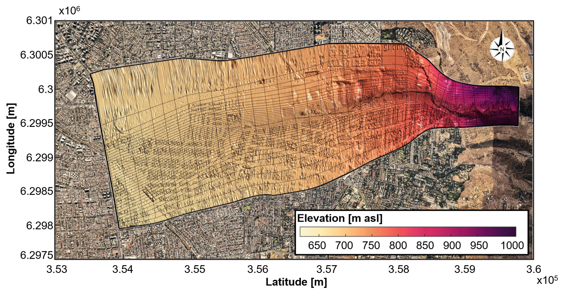
Figure 3 Aerial view of the urbanized area of the Quebrada de Ramón watershed. The area enclosed by the black line defines the computational domain used in the hydrodynamic model. The grid is presented every 100 nodes in the direction of the flow and every 20 nodes across the river channel. Background image: © Google Earth.

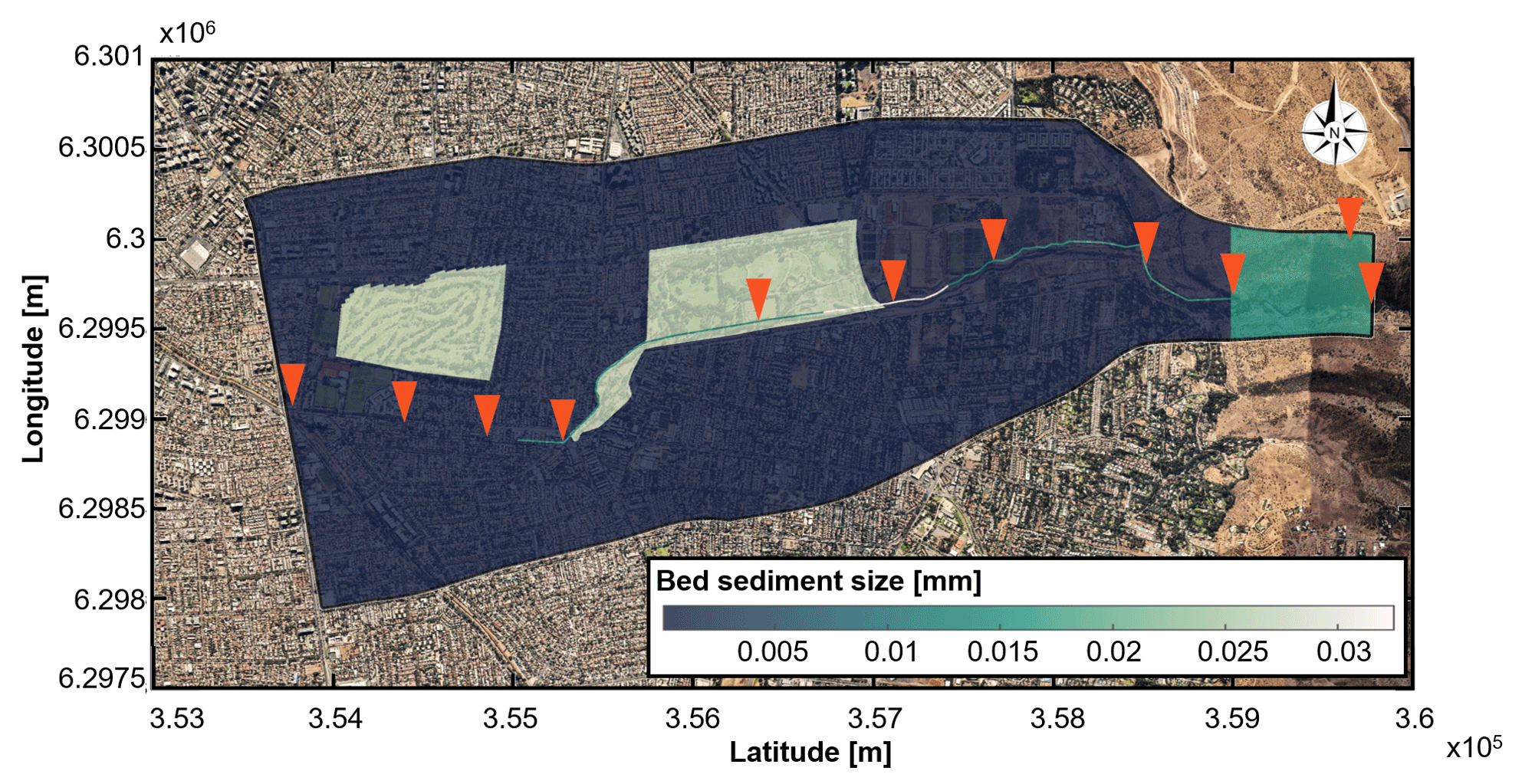
Figure 4 Distribution of the mean sediment size in millimeters. Orange triangles denote the sites where we performed direct measurements of sediment size distributions. Background image: © Google Earth.

For the Quebrada de Ramón watershed, we simulate the propagation of the 49 hydrographs obtained from the hydrological model, whose maximum flow rate exceeds 20 m³ s⁻¹, which is the maximum hydraulic capacity at the critical point in the urbanized area. We define the computational domain shown in Fig. 3 that comprises the channelized portion of the main channel (6.6 km approximately), which starts at an elevation of 878.8 m a.s.l. A curvilinear boundary-fitted grid is used to perform the simulations, consisting of a total of 3914×697 grid nodes. The grid resolution varies progressively in the flow direction from 0.5 m upstream to 2 m of resolution within the flooding zone. In the cross-stream direction, the resolution of the grid varies from approximately 0.5 m near the main channel to more than 30 m in areas that are never flooded. To construct the grid, we couple a 1 m resolution lidar survey of the area around the channel, with 0.5 m resolution topographic field measurements to define the main channel and a 0.5 m digital surface model (DSM) from satellite images for the rest of the watershed, which captures natural and built features.

The bed roughness is represented by a mean sediment grain diameter d_s, which is shown in Fig. 4. We use field measurements at the locations shown as the orange symbols to determine d_s along the channel. We derived values of d_s from Manning coefficients in the floodplain, by using the Strickler relation (Julien, 2010). Based on satellite images and field observations, we define two types of land cover: floodplain with short grass (n=0.025) in parks and rough asphalt (n=0.016) in the rest of the urbanized area.

The hydrographs resulting from the hydrological model correspond to the inflow boundary condition in the eastward boundary, and open boundary conditions are defined at all the other boundaries of the computational domain. The initial condition for all the cases is dry-bed since we are interested in simulating the propagation of single events, and the channel is typically dry before events. We run the simulations for a total physical time equivalent to the length of the hydrograph plus a time of concentration of the watershed (∼3 h). We use a simulation time step defined by the Courant–Friedrichs–Lewy (CFL) stability criterion, with values within 0.4–0.6.

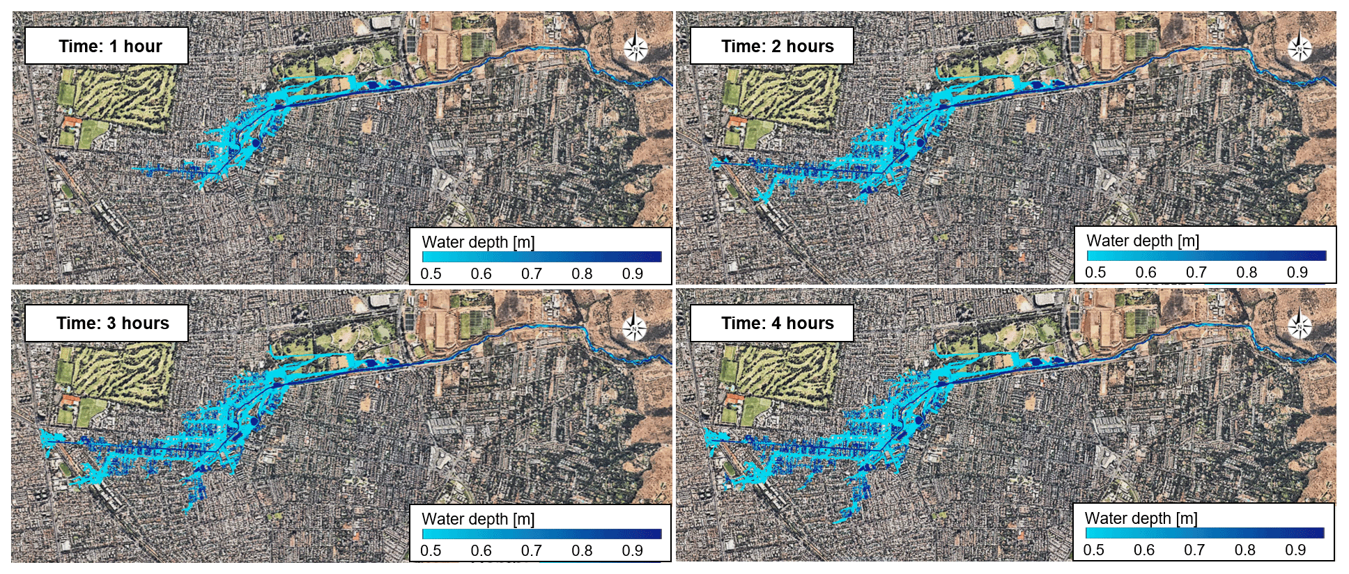
Figure 5 Instantaneous flow depth in the Quebrada de Ramón and the flooded area in Santiago, Chile, for a peak flow of 97 m³ s⁻¹ and 38 % of sediment concentration. Background image: © Google Earth.

The sediment transport is probably the factor with the most uncertainty, since its value can depend on localized landslides, previous recent storms, or inter-annual changes in the vegetation covering, among others. Magnitudes of sediment concentration have been reported for the largest flood registered in the watershed, which was generated during an abnormally warm storm, with periods of intense precipitation over partially saturated soils. The sediment concentration during the storm could not be directly measured, but it was estimated to be around 40 % (Sepúlveda et al., 2006; Sepúlveda and Padilla, 2008). In the present investigation, we chose values of sediment concentrations in a range between clear water and 40 %, through a Latin hypercube sampling. We based this range on estimations for previous events and a recent study in this river that shows the most significant differences in the hydrodynamics of the flow occur between 0 % and 20 % (Contreras and Escauriaza, 2020).

Figure 5 shows the instantaneous results of the simulations for a peak flow of 97 m³ s⁻¹ with 38 % of sediment concentration. The spatial and temporal resolution of the simulations allows us to explore in detail the evolution of the flow along the main channels and its propagation towards the urban areas. The results show significant changes in flow depth and velocity in the urbanized zone, with more gentle slopes that coincide with results reported in Contreras and Escauriaza (2020).

2.3 Definition of inputs and outputs of the surrogate model

Parameterizing the database and defining a small number of input and output variables that can capture the characteristics of the storms and the flood propagation require understanding the physics of the floods. In this section we provide a brief overview of the components that control flooding in Andean environments and define the parameters used to implement the surrogate model.

From the hydrometeorological perspective, the volume of precipitation and its spatial and temporal distribution are the critical factors that define the magnitude of the flood. Most of the precipitation in the region of study occurs between May and September, which constitutes the rainy season. Storms are typically frontal rainfall events that last from 1 to 2 d (Garreaud, 1993). They correspond to 80 % of the total events in the area, accumulating 50 % of the annual precipitation (Montecinos, 1998). Cyclonic events, however, also take place in the mountains, producing storms with intense precipitation. While these events occur occasionally in the area, they can produce extreme flash flooding. El Niño–Southern Oscillation (ENSO) is one of the factors that also generates floods in the Andes (García, 2000; Sepúlveda et al., 2006). This phenomenon cyclically produces years of severe drought or frequent floods (Rutllant et al., 2004). During rainy years, also known as El Niño years, the intensity and duration of the storms are larger, often producing flash floods and debris flows in the watersheds along the Andean range.

Warm temperatures during storms, especially when they are influenced by the ENSO phenomenon, are a critical factor that might increase the flooding effects (Vicuña et al., 2013). Due to the complex topography in these environments, watersheds are very susceptible to the variation in the elevation of the 0 ^∘C isotherm. Warm conditions enlarge the total area contributing direct excess runoff, increasing runoff volumes, peak discharges, flow velocities, and sediment transport.

Steep topographic gradients of the channels promote the mobilization of large amounts of sediments, mostly from landslides. In many cases, the volumetric sediment concentrations in the flow can exceed 20 %, which requires the consideration of additional stresses produced by the particle–flow and particle–particle interactions (Julien, 2010). In those cases, the rheology of the flow changes from the traditional resistance term that only considers the bed stresses. The changes in the flow hydrodynamics due to high sediment concentrations are also evident in the flood propagation. In the study region, Contreras and Escauriaza (2020) showed that the flooded area in the urban zone increases 36 % when comparing the same flood with clear water or 20 % sediment. Likewise, the water depth in the urban area can increase 25 % when 60 % of sediment concentration is considered instead of clear water.

In this framework, we characterize the extreme events in the watershed by only four parameters to define the storms. These parameters are the following:

1. mean value of the intensity of rainfall per event $\stackrel{\mathrm{‾}}{P}$;

2. the second statistical moment of the precipitation $M_{{\mathrm{2}}_{\mathrm{P}}}$ with respect to the starting time of each event, to incorporate the temporal distribution and duration of the event;

3. the minimum temperature during the day of the event T_Min, which yields information on the elevation of the 0 ^∘C isotherm; and

4. sediment concentration (C), to consider the volumetric and rheological effects of the flood, i.e., the changes of velocity and depth, especially when we have a hyperconcentrated flow.

The output of the surrogate model can be any variable derived from the time series of water depth or flow velocity distributed in space (i.e., water depths, flow velocities, discharge, force). Here we select the maximum water depth at the location where the channel reduces its hydraulic capacity to 20 m³ s⁻¹. Thus, the vector of inputs X and the output Y to implement the surrogate model are encoded as follows,

$$\begin{array}{}\text{(4)}& X=\left[\begin{array}{cccc}\stackrel{\mathrm{‾}}{P}& M_{{\mathrm{2}}_{\mathrm{P}}}& T_{\mathrm{Min}}& C\end{array}\right];Y=\left[h_{\mathrm{Max}}\right].\end{array}$$

In the next section we explain the statistical procedure to create new scenarios from the interpolation of precomputed cases of the database.

3 Surrogate model: kriging on the parameter space

After constructing the database with 49 simulations of different storms, and parameterizing them by defining the inputs and the output of the simulations, we implement the surrogate model by defining a simplified relationship among the variables. In this case we use DACE (Design and Analysis of Computer Experiment), a MATLAB toolbox designed to implement a variety of kriging models and extensions for surrogate formulations (Couckuyt et al., 2014).

In general terms, kriging considers the response of the model $\widehat{Y}\left(X\right)$ to a vector of inputs X=[x¹, x², x³, …, x^d] as a linear combination or regression function f(X) that captures the general trend of the data and a random function R(X) that describes the residuals of the stochastic process (Lophaven et al., 2002):

$$\begin{array}{}\text{(5)}& \widehat{Y}\left(X\right)=f\left(X\right)+R\left(X\right).\end{array}$$

Defining the correct regression function is not a simple task, since this function should capture the complexity in the input–output relationship. DACE provides several options, and for simplicity the most used ones are the simple and the ordinary kriging, in which the regression function is defined as a zero-order or constant function, respectively. In this investigation we use universal kriging, which provides more flexibility to the regression function and defines f(X) as a linear combination of p chosen functions, as follows:

$$\begin{array}{}\text{(6)}& f\left(X\right)=\sum _{i=\mathrm{1}}^p{\mathit{\alpha }}_i{b}_i\left(X\right),\end{array}$$

where b_i(X) represents the basis functions, and α_i represents arbitrary coefficients. Assuming that the values of α_i are correctly determined by generalized least squares (GLS), the random function R(X) becomes white noise, and it can be represented by a Gaussian process Z(X) with mean 0, variance σ², and a correlation matrix Psi (Lophaven et al., 2002). Thus, the formulation of the surrogate model can be written as

$$\begin{array}{}\text{(7)}& \widehat{Y}\left(X\right)=f\left(X\right)+Z\left(X\right).\end{array}$$

Implementing a surrogate model requires a matrix with n samples S=[s₁, s₂, s₃, …, s_n]^T, with s_i∈ℝ^d, and its respective deterministic or high-fidelity responses Y=[y₁, y₂, y₃, …, y_n]^T with y_i∈ℝ^q. To determine the functions b_i(X) in the regression function, we assume that they are power-based polynomials of degree 0, 1, or 2 and that they are encoded in the matrix $\mathbf{F}(i,j)=b_j\left({\mathit{s}}_i\right)$ with $i\in \mathit{\{}\mathrm{1},n\mathit{\}}$, $j\in \mathit{\{}\mathrm{1},p\mathit{\}}$.

On the other hand, the Gaussian process Z(X) is defined by the correlation matrix $\mathrm{\Psi }(i,j)=\mathit{\psi }({\mathit{s}}_i$, s_j) with $(i,j)\in \mathit{\{}\mathrm{1},n\mathit{\}}$. Each term of the matrix is computed from a stationary correlation function (Couckuyt et al., 2013):

$$\begin{array}{}\text{(8)}& \mathit{\psi }\left({\mathit{s}}_i,{\mathit{s}}_j\right)=\exp \left(-\sum _{a=\mathrm{1}}^d{\mathit{\theta }}_a\left|{\mathit{s}}_i\right(a)-{\mathit{s}}_j(a){|}^k\right),\end{array}$$

where θ_a and k are parameters that can be fixed or determined by using a maximum likelihood estimation (MLE) depending on the correlation function chosen. DACE has built-in multiple options for the correlation functions: Gaussian, exponential, cubic, linear, spherical, spline, Matérn-3/2, or Matérn-5/2.

The mean and standard deviation of the prediction are estimated as

$$\begin{array}{}\text{(9)}& \begin{array}{rl}& \widehat{Y}\left(\mathit{X}\right)=\mathbf{M}\mathit{\alpha }+\mathit{r}\left(\mathit{X}\right){\mathrm{\Psi }}^{-\mathrm{1}}(Y-\mathbf{F}\mathit{\alpha }),\\ & s=\mathit{\sigma }\sqrt{\mathrm{1}-\mathit{r}\left(\mathit{X}\right){\mathrm{\Psi }}^{-\mathrm{1}}\mathit{r}(\mathit{X}{)}^T+{\displaystyle \frac{\mathrm{1}-{\mathbf{F}}^T{\mathrm{\Psi }}^{-\mathrm{1}}\mathit{r}(\mathit{X}{)}^T}{{\mathbf{F}}^T{\mathrm{\Psi }}^{-\mathrm{1}}\mathbf{F}}}},\end{array}\end{array}$$

where M is the matrix F of basis functions evaluated in the input vector X, and r(X) is a vector of correlations r(X)=[ψ(X, s₁), ψ(X, s₂), …, ψ(X, s_n)]. In the following sections we use the mean as the prediction (h_P) and its standard deviation s as parameters to assess the performance of the model. Lophaven et al. (2002) and Couckuyt et al. (2013) provide a detailed description of the universal kriging in DACE, which is used here.

4 Results

4.1 Cross-validation process: implementing the surrogate model

Determining the correct order of the regression function and the correlation function is critical to optimize the accuracy of the surrogate model. Since there is no clear methodology to define them, we implement a cross-validation process to assess the accuracy of a surrogate model built with multiple combinations of regression and correlation functions.

Traditionally, the cross-validation process consists of dividing the database into two groups. The first set is used to implement the surrogate model and the second one to validate the results and evaluate the accuracy of the predictions. In this research, due to the lack of hydrometeorological and streamflow data, we only have simulations for 49 storms that produce the critical conditions for the system. Thus, reducing the number of storms in the database might significantly affect the accuracy of the model. To deal with this setback, we run the cross-validation process by selecting one testing storm at a time, building the surrogate model with the remaining 48 storms.

We evaluate the performance of the model based on the mean square error (MSE) and the percent of cases in which the high-fidelity value is within 1 standard deviation from the mean of the prediction (PWSD), considering the definition of $\widehat{Y}\left(\mathit{X}\right)$ and s in Eq. (9). In the analysis we use the water depth at the point in the urban area where the hydraulic capacity of the channel reduces to 20 m³ s⁻¹. We tested three orders of the regression function (orders 0, 1, and 2) and the nine correlation functions (cubic, exponential, Gauss, Gauss-p, linear, Matérn-3/2, Matérn-5/2, spherical, and spline).

Figure 6 shows the performance for the 27 different surrogate models. The MSE, on the left, is significantly reduced when we use a zero- or first-order regression function, in comparison with the second order, but it does not strongly depend on the correlation function. On average, the MSE for the second-order regression function is 18.59 %, and it decays to 2.92 % and 2.51 % for zero- and first-order functions, respectively. In terms of the PWSD, the performance of the different regression functions is associated with the correlation function as well. For the case of a zero-order function, we observe the worst performance of the model for Matérn-5/2 (PWSD = 77 %) and the best one for a cubic or spline function (PWSD = 90 %). For a first-order function, the Gauss and the cubic or Gauss-p yield the best and the worst results, respectively, with PWSD = 75 % and 90 %. For the second-order function, in general, the value of PWSD is larger for all the correlation functions. The worst cases get over 85 % and the best ones, Gauss and Matérn-5/2, up to 90 %.

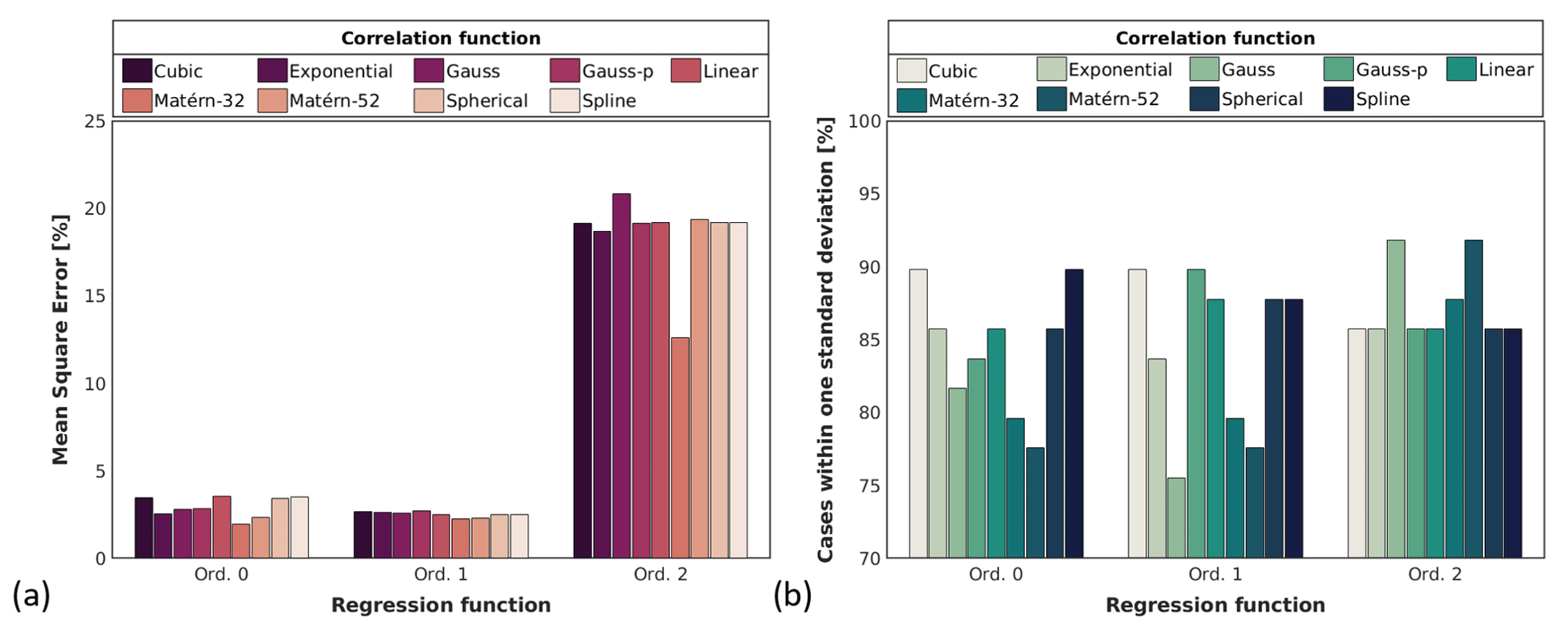
Figure 6 Assessment of the surrogate model built with all the available combinations of regression and correlation functions. Panel (a) shows the performance in terms of the mean square error and (b) the percentage of cases predicted within 1 standard deviation.

Based on the significant differences of MSE with the regression functions, we decide to implement the surrogate model with the best combination of MSE and PWSD but only considering the zero- and first-order regression functions. We notice that the linear correlation function reaches the minimum MSE for both orders of regression functions. Besides, this obtains one of the highest PWSDs, only surpassed by the Cubic and the Gauss-p functions for 2.5 %.

Thus, we use a surrogate model built with a first-order regression function and a linear correlation function for the entire upcoming analysis. The next subsection shows how this surrogate model performs in terms of the relative and absolute error and how the different input parameters affect the accuracy of the predictions of water depth at the specific critical point in the urban area. Then, we explore the idea of a surrogate model distributed in space to predict flooded areas.

4.2 Prediction of maximum water depth at the critical point

We study the performance of the surrogate model built with a first-order regression function and a linear correlation function for specific events. We use the same methodology to run the cross-validation process in the previous subsection and examine the absolute and relative error of the prediction. We aim at understanding when the surrogate model performs the best and the poorest depending on the characteristics of the storms.

Figure 7a shows in red the absolute error between the high-fidelity value and the mean of the prediction for each of the 49 storms. The mean of the absolute error is 0.13 m, with a minimum of only 0.0064 m (Event 27) and a maximum that increases to 0.73 m (events 1 and 48). The majority of the events have an error equal to or smaller than 0.25 m (44 storms or 89.8 %), 6.12 % is in the range 0.25–0.5 m, and only two of the events, 4 %, have an error that exceeds 0.5 m. The blue bars represent 1 standard deviation of the prediction plotted in the positive and negative directions around zero. Their values vary from a minimum of 18.24 cm to a maximum of 82.78 cm, with a mean of 29.21 cm. Even though 87.76 % of the predictions are within 1 standard deviation, we observe that there is an association between the high standard deviations and larger errors.

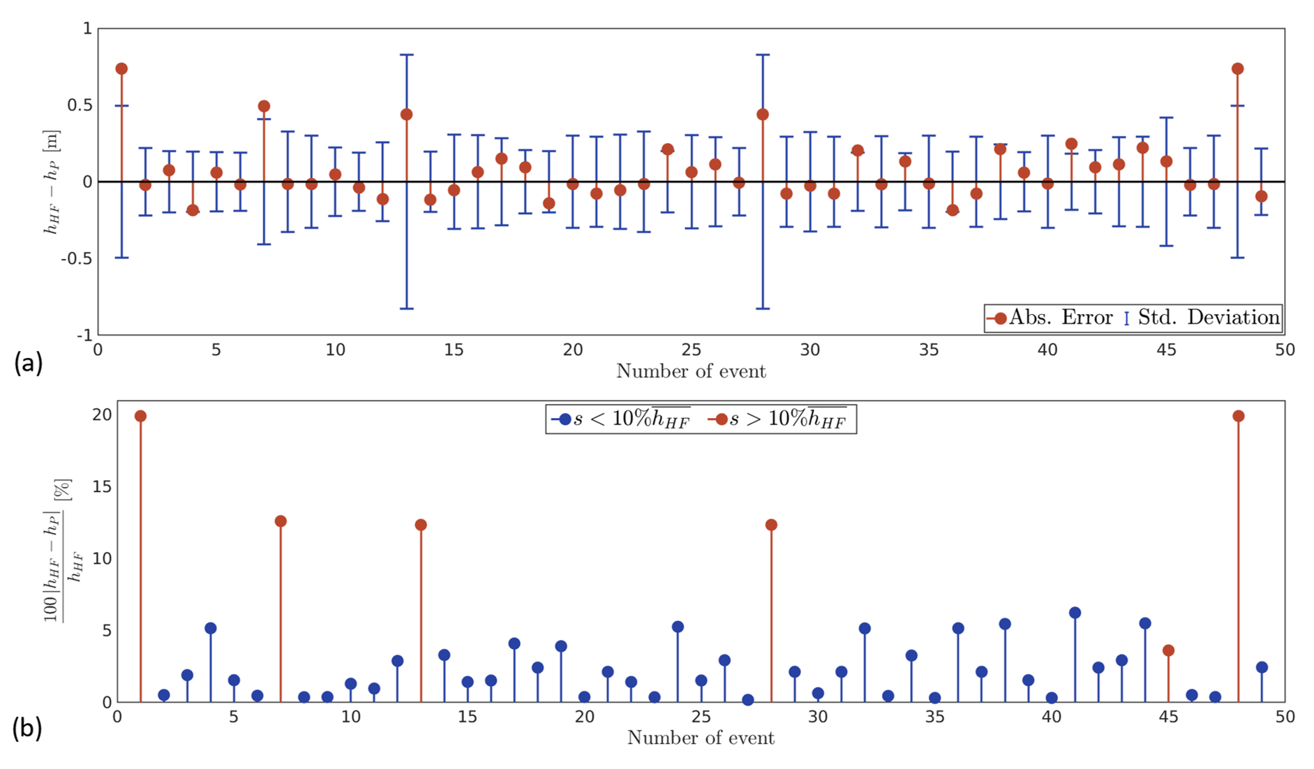
Figure 7 Results of the surrogate model for the water depth, compared to the data obtained from the high-fidelity approach. Panel (a) shows in red the absolute error between the high-fidelity value and the mean of the prediction and in blue 1 standard deviation of the prediction around zero. Panel (b) shows the relative error of the model. The events in red represent those with a predicted standard deviation larger than 10 % of the mean maximum water depth at the point of the predictions for the entire set of high-fidelity values $\stackrel{\mathrm{‾}}{h_{\mathrm{HF}}}$.

We compare these results with a similar model developed by Bermúdez et al. (2018). They implemented a surrogate model based on regression functions to predict maximum water depth at three specific points in a coastal basin. After running 100 high-fidelity hydrodynamic simulations, they estimated a mean absolute error for the water depth of 0.023 m. This is an order of magnitude lower than our mean error (0.13 m). We explain this difference based on the inputs used to implement the surrogate models. While we use hydrometeorological data and thus we intend to substitute the combination of hydrological and hydrodynamics high-fidelity simulations, Bermúdez et al. (2018) uses the maximum discharge at the inlet and the water elevation at the outlet, so the surrogate model only replaces the hydrodynamic propagation model.

We also plot in Fig. 7b the relative error for each of the events, and we highlight with red those with a standard deviation higher than 10 % of the mean of the maximum water depth at the point of prediction, for the total 49 storms. The mean of the relative error for all the events is 3.6 %, with a minimum and maximum equal to 0.18 % and 19.92 %, respectively. However, if we consider a valid prediction as those values with s≤10 %$\stackrel{\mathrm{‾}}{h_{\mathrm{HF}}}$, we can establish that the surrogate model can predict 87.76 % of the storms, with a mean, minimum, and maximum relative error equal to 2.22 %, 0.18 %, and 6.24 %, respectively.

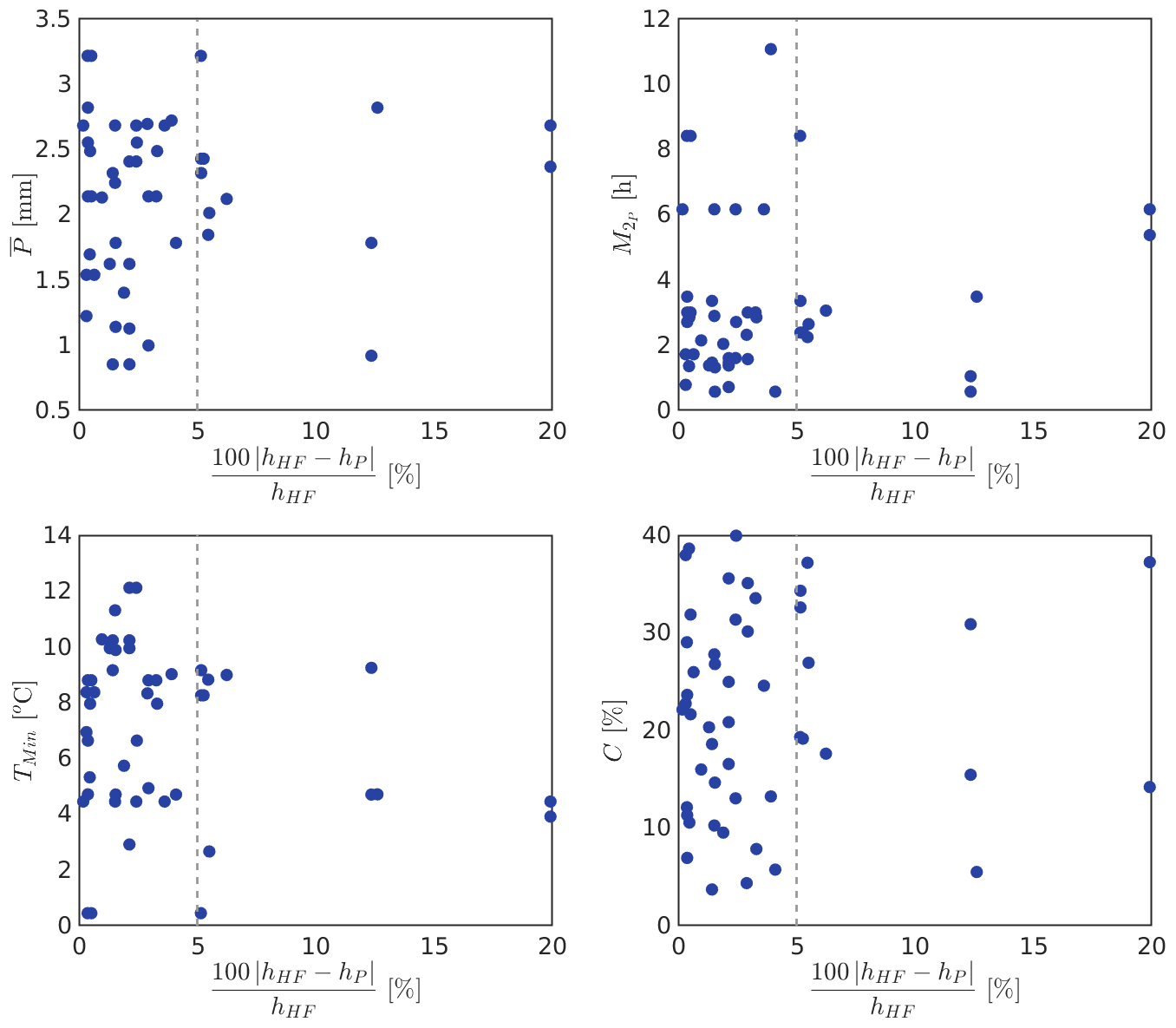
Figure 8 Results of the surrogate model for the four input parameters (P, $M_{{\mathrm{2}}_{\mathrm{P}}}$, T_Min, and C), compared to the data obtained from the high-fidelity approach.

We also focus on understanding how the surrogate performs depending on the characteristics of the storms. In Fig. 8, we plot the relative error as a function of the four input parameters $X=\left[\stackrel{\mathrm{‾}}{P}{M}_{{\mathrm{2}}_{\mathrm{P}}}{T}_{\mathrm{Min}}C\right]$ for each of the 49 storms.

Figure 8a shows that the two predictions with more than 10 % of relative error are events with $\stackrel{\mathrm{‾}}{P}>\mathrm{2}$ mm. This could suggest that the surrogate model loses accuracy for intense storms; however, the model is also able to predict storms with $\stackrel{\mathrm{‾}}{P}>\mathrm{3}$ mm and errors that do not exceed 5 %.

We show the magnitude of $M_{{\mathrm{2}}_{\mathrm{P}}}$ in Fig. 8b, as a representation of the temporal distribution of precipitation for the total duration of the storms. The performance of the model does not depend strongly on the values of the second moment of precipitation. Two predictions with relative errors larger than 10 % are storms with $M_{{\mathrm{2}}_{\mathrm{P}}}$ on the order of 6 mm², over the average of the parameter in the database. Nevertheless, four other predictions with similar values of $M_{{\mathrm{2}}_{\mathrm{P}}}$ and three others with $M_{{\mathrm{2}}_{\mathrm{P}}}>\mathrm{8}$ have relative errors that do not exceed 5 %.

Warm temperatures during storms have increased the flooding effect by increasing the total area draining liquid precipitation, runoff volumes, and peak discharges. In Fig. 8c, we show that the surrogate model exhibits good performance at predicting storms with minimum temperatures that exceed 10 ^∘C, with relative errors lower than 5 %. Indeed, the two storms with the largest relative error (∼20 %) occur under low temperatures (<5 ^∘C).

The sediment concentration, shown in Fig. 8c, does not have a specific relationship with the magnitude of the relative error either, since the predictions with errors that are larger than 10 % take place in events with sediment concentrations in almost the entire range of possible values (0 %–40 %).

Therefore, we do not observe that the surrogate model does especially good or bad for specific characteristics of storms, which we consider a valuable property of the model. Having a lightly uniform distribution of cases in the database is highly recommended; thus the model could accurately predict events that do not occur very often.

We also study the relationship between the accuracy of the model and the magnitude of the flood, through the maximum discharge at the prediction point, Q_Max, as shown in Fig. 9. While the range of Q_Max in the database varies between 20 and 46 m³ s⁻¹, the predictions with relative errors greater than 10 % are floods with $Q_{\mathrm{Max}}<=\mathrm{40}$ m³ s⁻¹. More specifically, the two cases with error of ∼20 % do not exceed a discharge of 35 m³ s⁻¹. Another relevant result is that the surrogate model shows excellent performance in predicting extreme floods. For example, the largest flood, with a maximum discharge of ∼46 m³ s⁻¹, is predicted with a relative error that is lower than 1 %.

Figure 9 Results of the surrogate model for the flow discharge, compared to the data obtained from the high-fidelity approach.

In terms of efficiency and computational cost, the time required for building the model is highly dependent on the number of cases in the database. For the case of 49 scenarios, the time required for estimating the parameters is 4.78 s, which needs to be done only once. We can later predict the maximum water depth at a specific point almost instantaneously. Conversely, coupling the hydrologic and hydrodynamic models takes on the order of days. Since the hydrological model can run only in a single core, running the 200 years of continuous simulation takes about 2 d. Then, we have to post-process the data to select the single storms, which takes about an hour. Finally, we run the high-fidelity hydrodynamic model, which takes between 2 and 3 d to complete using 120 cores. Therefore, running the hydrologic model only for a few computation days, coupling it with the hydrodynamic model, and predicting water depth would never take less than 2 d. This is orders of magnitude longer than the seconds or minutes that predicting with the surrogate model takes.

4.3 Predicting the flooded area

With the objective of taking advantage of the high-resolution results from the database of high-fidelity simulations, we also explore the idea of predicting the total flooded area in the urban zone. We implement an individual surrogate model at each point in the domain, which predicts the maximum water depth at the specific location by using a first-order regression function and a linear correlation function. To develop the local surrogate models, we consider the same vector X as the input parameter and the maximum water depth at each point of the domain as the output. Then, we use in parallel the set of surrogate models for a unique set of input values, generating a map of the maximum flooded area, by using the maximum water depth predicted at each point of the domain.

We validate the model through the same cross-validation process described in Sect. 4.1. We build the surrogate model with 48 of the 49 storms, and we validate the prediction with the remaining storm. We iterate this process for all the storms. Due to the wide variety of storms that compose the database, results show areas that are rarely flooded are often predicted as flooded with water depths on the order of 10⁻² cm. To deal with this effect, we filtered the predictions, considering flooded areas to be the zones with maximum water depth equal to or larger than 10 cm.

We assess the performance of this method as a qualitative error, as shown in Fig. 10 for a specific storm with $X=\left[\mathrm{3.22}\mathrm{mm}\mathrm{8.42}{\mathrm{mm}}^{\mathrm{2}}\mathrm{0.45}{}^{\circ }\mathrm{C}\mathrm{29.05}\mathit{\%}\right]$ and Q_Max=23.7 m³ s⁻¹. In the figure, the green area represents nodes where the surrogate model and the high-fidelity simulation show equal flooding, the orange zone shows the nodes where the high-fidelity model shows flooding which is not predicted by the surrogate model, and conversely the blue area shows where the surrogate model predicts flooding in sections that are dry from the high-fidelity model solutions.

Figure 10 Qualitative error to assess the performance of a set of surrogate models working in parallel to predict flooded area in the study area. The results correspond to a randomly selected storm with the input parameters P=3.22 mm, $M_{{\mathrm{2}}_{\mathrm{P}}}=\mathrm{8.42}$ mm², T_Min=0.45 ^∘C, and C=29.05 %. The green area is where the surrogate model correctly predicts the flooding, the orange shows zones where the surrogate model does not predict the flood, and the blue color represents zones where the surrogate model predicted flood but the high-fidelity model does not. Background image from © Google Earth.

Since this is a mountain river with a steep slope, the flooded area is usually very narrow along the main channel. The flooded nodes in this section are always correctly predicted by the surrogate model. In Fig. 10, the over- and under-predicted regions exhibit water depths that are very close to the 10 cm threshold, which indicates that we could explore a better filter for future analysis.

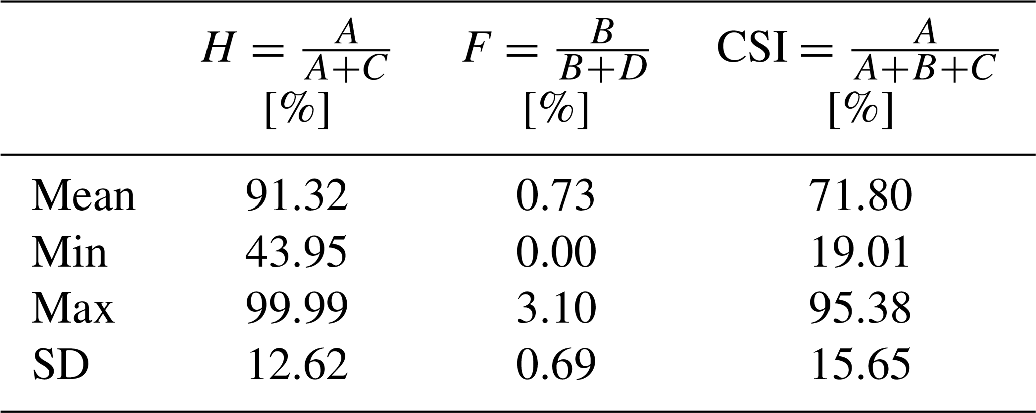
Additionally, following the guidelines and definitions in Stephens et al. (2014), we computed three metrics to evaluate the performance of the model: (1) hit rate (H), which represents the fraction of the flood area correctly predicted; (2) false alarm rate (F), which is the fraction of dry areas incorrectly predicted; and (3) critical success index (CSI), which represents the ratio between the correctly predicted flooded area and the total estimated flooded area. Table 1 shows the equations for each parameter, where A is the flooded area correctly predicted, B is the area over-predicted, C the area under-predicted, and D the correctly estimated dry zones. We show the mean, minimum, maximum, and standard deviation for the set of storms. For H and F, the ideal results would be 100 % and zero, respectively. The mean values of H and F indicate that the model tends to underestimate the flooded zones.

Table 1 Quantitative assessment of the surrogate model for predicting flooded areas. We present the hit rate (H), false alarm rate (F), and critical success index (CSI). The values represent the basic statistical parameters for the 49 storms.

In terms of efficiency, building this model requires 2 h with the current database of 49 cases. The number of outputs is equivalent to the number of nodes in the discretization of the high-fidelity hydrodynamic model, which is 2 728 058 nodes. It is important to note that this process needs to be done only once; then the prediction for different scenarios is quasi-instantaneous.

5 Discussion

In this investigation we develop the first surrogate model applied to rapid flood events in mountain regions. We focus on assessing the performance and applicability of this type of model in Andean regions, with complex generation and propagation of floods, and poorly monitored. The results can also contribute to identify some considerations for future applications guided to operational systems for water depth and flooded area predictions.

In terms of implementing the model, the accuracy of results is highly related to the quality and size of the precomputed database: having a good representation of the physics of flood propagation to perform high-fidelity simulations determines the base error of all the predictions. From the hydrological standpoint, we use a continuous rainfall–runoff model implemented in HEC-HMS, which is one-way coupled with the high-resolution two-dimensional hydrodynamic model to solve the propagation of the flood over the urbanized area. In this aspect, using field measurements to calibrate and validate both models, including additional physical phenomena that might have significant effects in other rivers such as the erosion and deposition of sediments, and having a better description of spatially distributed parameters (for instance friction coefficients and land use changes, among others) can contribute to improve the accuracy of the high-fidelity models. In this sense, we must clarify that all the errors analyzed in this research are only associated with the prediction of the surrogate model, but we do not include the error of the high-fidelity results, since it is unrealistic to have detailed measurements for every storm at each location of a city.

Another important step is building a database that is broad enough to cover the entire range of possible cases, and with a sufficient number of storms to provide a robust set of events for the interpolation method. Since the surrogate model is based on kriging, predicting cases outside the range of parameters simulated for the database can lead to results that are completely controlled by statistical errors. This is particularly relevant for the most extreme low-frequency floods, but having a good representation of them in the database is crucial to predict them. For operational purposes, a broader set of precomputed storms is required in order to have two different sets of data to cross-validate the surrogate model. However, since the record of precipitation in the study area is not long enough, synthetic storms might be required for regions with limited information.

To calibrate the surrogate model, we choose the best combination of regression and correlation functions based on the mean square error and the percent of cases predicted within 1 standard deviation. The significant difference between the results for a zero- or first-order regression function versus the second-order function shows that a linear function can capture the primary trend between inputs and outputs, and the correlation function provides the fluctuations from the structure of the statistical linear dependence. Over-constraining this relationship to a quadratic function results in a deterioration of the results of the surrogate approach. The different correlation functions seem to be more flexible to represent the noise associated with the regression function.

To study the performance of the surrogate model to predict water depths at specific points in the watershed, we use a model built with a first-order regression function and a linear correlation function. From the results, we can clearly select events that are correctly predicted by the surrogate models in terms of relative and absolute error. They correspond to the ∼90 % of the predictions, with absolute and relative errors smaller than 0.25 m and ∼6 %, respectively. On the other hand, we observe that the remaining ∼10 % of the events are predicted with very significant errors that reach 0.73 m or a ∼20 % relative error. We notice the association between low accuracy and high values of the standard deviation of the prediction s. We suggest considering this relationship to distinguish events that are not captured by the model. While not predicting all the events is a limitation for operative-oriented models, we consider it to be a positive outcome that based on the value of the standard deviation we can determine whether the prediction is correct. In this sense, more sophisticated filters can be applied to determine the accuracy of the predictions, but our observations show that the model yields significantly larger standard deviations of the prediction s when the event is not correctly predicted. Additionally, the short computational times used to predict single-point water depths allow us to assess different combinations of inputs that might contribute to identify outliers in the predictions.

We must also mention that the current database is built based on the historical record of events in the study area. This means the events are not uniformly distributed in the entire range of possible values for each input. In fact, the events that are the most represented in the database have maximum flow rates at the critical point lower than 35 m³ s⁻¹; therefore they are not the most destructive storms. For this reason, we study whether specific values of the input parameters or maximum flow rate at the prediction point might diminish the accuracy of the prediction, and we do not see that specific storms are consistently not predicted by the model. On the contrary, we highlight that the current database is able to predict frequent but also infrequent storms, with high values of $\stackrel{\mathrm{‾}}{P}$, $M_{{\mathrm{2}}_{\mathrm{P}}}$, T_Min, and Q_Max. This shows that a uniformly populated database is recommended but might not be required, as long as the entire range of possible cases is precomputed.

We predict flooded areas to try to take advantage of the spatially distributed information in the database. Our approach, estimating the maximum water depth at each point of the domain, presents new challenges since the prediction of each node does not consider the condition of surrounding points, and discontinuities in the water surface might be predicted. In addition, this methodology does not accurately predict very shallow water depths. The wide variety of storms influences the prediction of water depth at points that are rarely flooded, oftentimes with values on the order of a millimeter or less. We propose solving this by applying a filter that neglects all the flooded zones with water depths shallower than 10 cm, which works for mountain regions where the slopes are steep, as in the study case. However, there can be significant differences in the flooded area predicted for different values of the filter, especially during larger floods that reach flatter areas or watersheds characterized by very flat floodplains. In those cases, we suggest for future applications assessing different approaches that they incorporate information of surrounding points. Thus, we only do a qualitative analysis to determine whether the areas could potentially be flooded, which is enough for quick-response systems. In terms of efficiency, this methodology provides the quasi-instantaneous response the surrogate models seek to provide.

In general terms, the main advantage of this statistical approach is to produce fast scenarios for decision makers, obtained directly from the characteristics of the meteorological event with no need of the high-fidelity approach, which requires running the computationally expensive hydrological and hydrodynamic models. While the accuracy of the prediction is affected by the statistical approach, the low errors of most of the prediction allow thinking on possible applications for quick-response systems, specially if a highly populated database that covers the entire range of possible storms is used.

However, we are aware of some of the limitations of this methodology. First, since the region is poorly monitored, and there are very scarce historical hydrologic and streamflow data, a more robust database must include synthetic storms. Additionally, to deal with the lack of information regarding sediment concentration, we suggest including as part of the database the same events with different concentrations. This might contribute to improve the accuracy of predictions when assessing a storm with different potential concentrations. For the long term, applications would need to include updates of the database, especially in the context of continuous modifications of the topography and land use. The replicability of this methodology to other watersheds might not be an easy task. While we can use the same interpolation methods in other watersheds, we would need to implement the high-fidelity models with the local data and build a new database, which is by far the most time-consuming and computationally expensive step. Additionally, depending on the local physics of the study area, the inputs and outputs of the surrogate model (X and Y) might need to be redefined as well.

6 Conclusions

The simulation of flood hazards by extreme precipitation in mountain streams requires numerical models capable of capturing complex flows that are influenced by the geomorphic features of the channel and by high sediment concentrations that are common in these regions. In this investigation we develop two models for simulating the flow in an Andean watershed in central Chile: (1) a hydrologic model combined with a 2D hydrodynamic model that is coupled with the sediment concentration in mass and momentum and (2) a surrogate model that employs precalculated scenarios of the previous models, to interpolate new cases using kriging.

With the combination of the hydrological and hydrodynamic models, we can capture the complexity of the flows and estimate accurate responses to different storms. However, they require expensive computational resources and many CPU hours, which cannot be a tool suited for real-time predictions. We propose using surrogate models to reduce the computational cost, provide a fast prediction, and evaluate different scenarios to deal with the uncertainty of different future conditions, while preserving the effect of the physics of the flows in the prediction. To develop this surrogate model, we characterize the extreme flood events by statistical parameters of the storm (see Contreras and Escauriaza, 2020, for details), and by the sediment concentration. We develop a database of 49 storms by using the high-fidelity hydrological and hydrodynamic models. We perform kriging interpolation, based on the precomputed database, to obtain water depth at a critical point in the domain and flooded areas.

Results show a promising performance of the surrogate models for water depth prediction at a critical point in the domain. The current database can describe the flow propagation of floods, incorporating the connection of the hydrology and the complex hydrodynamics of the flow, highly affected by rapid slope variations and high sediment concentrations. Despite having only 49 storms measured in the entire historical record of the study area, the surrogate model can predict 90 % of the storms with errors lower than 6 % or 0.25 m. The remaining 10 % of the storms are clearly not predicted, based on the high values of the standard deviation of the prediction. More importantly, the surrogate model shows good predictions for the most extreme events, with high values of mean precipitation, minimum temperature, storm duration, and peak flow, which are sparsely represented in the current database. This shows that the most critical factor to design the database is covering the entire spectrum of possible storms, rather than the uniformity of the storm representation in the database.

The implementation of surrogate models to predict flooded areas needs a more careful processing of the results. Since using individual surrogate models to predict maximum water depth at each point of the domain does not consider the influence of surrounding points, discontinuities in the water surface can emerge in the map. However, our results show that this could be a powerful tool to qualitatively predict flooded areas, especially in mountain rivers where changes of the water depths and the location of the wet–dry interface are more abrupt and easier to identify, compared to smoother topographies.

In the future, this surrogate approach can be considered for a real-time automated forecast framework and as an advanced tool for decision makers and stakeholders, who can evaluate scenarios without the technical expertise on the calculation of complex flows during extreme hydrometeorological events. However, some important issues need to be resolved first: we recommend increasing the high-fidelity database by using synthetic storms distributed with methods such as the Latin hypercube sampling. This will improve the cross-validation process to determine the regression and correlation function, and it will also improve the accuracy of the predictions, as the interpolation model will have more information to estimate cases that have not been precomputed. In addition, we will test more sophisticated filters to improve the predictions and clean areas of the map with almost zero water depth, which also acquire great importance on flatter watersheds. Other future topics of research include the incorporation of the time dependence, to predict water depths at different times during storm events. This new feature will present new challenges since the database has been built with storms of different durations; therefore a normalization of the storm durations will be required.