the Creative Commons Attribution 4.0 License.
the Creative Commons Attribution 4.0 License.
 | 27 Nov 2020
Including informal housing in slope stability analysis – an application to a data-scarce location in the humid tropics
Elisa Bozzolan
Elizabeth Holcombe
Francesca Pianosi
Thorsten Wagener
Empirical evidence from the humid tropics shows that informal housing can increase the occurrence of rainfall-triggered landslides. However, informal housing is rarely accounted for in landslide hazard assessments at community or larger scales. We include informal-housing influences (vegetation removal, slope cutting, house loading, and point water sources) in a slope stability analysis. We extend the mechanistic model CHASM (Combined Hydrology and Stability Model) to include leaking pipes, septic tanks, and roof gutters. We apply this extended model (CHASM+) in a region of the humid tropics using a stochastic framework to account for uncertainties related to model parameters and drivers (including climate change). We find slope cutting to be the most detrimental construction activity for slope stability, and we quantify its influence and that of other destabilising factors. When informal housing is present, more failures (+85 %) are observed in slopes that would otherwise have had low landslide susceptibility and for high-intensity, short-duration precipitations. As a result, the rainfall threshold for triggering landslides is lower when compared to non-urbanised slopes and comparable to those found empirically for similar urbanised regions. Finally, low cost-effective “low regrets” mitigation actions are suggested to tackle the main landslide drivers identified in the study area. The proposed methodology and rainfall threshold calculation are suitable for data-scarce contexts, i.e. when limited field measurements or landslide inventories are available.
- Article
(6256 KB) - Full-text XML
-
Supplement
(825 KB) - BibTeX
- EndNote


Global and regional landslide records reveal an increase in rainfall- and human-triggered landslides during the last century, mainly in economically developing countries with rapid population growth and urbanisation (Kirschbaum et al., 2015; Froude and Petley, 2018). This increase might be partly due to continuing improvements in landslide recording, but it also indicates the growing impact of climate and urban pressure on landslide occurrence (Larsen, 2008). Understanding the mutual interactions between the natural and urban environment becomes particularly relevant in the humid tropics, where high-intensity and long-duration rainfall events are the main landslide triggers, and urban expansion is poorly regulated (Lumb, 1975; UN-Habitat, 2015). The natural landslide susceptibility of these regions coupled with the lack of urban planning and regulations can increase risk in terms of not only vulnerability and exposure but also hazard.
Potential anthropogenic landslide drivers include slope cutting and filling for house and road construction (Sidle and Ziegler, 2012; Smyth and Royle, 2000), slope degradation with clearance of forested areas (Gerrard and Gardner, 2006; Vanacker et al., 2003), inadequate drainage networks, unplanned redirection of storm run-off, and poorly maintained septic systems (Diaz, 1992; Anderson et al., 2008). In this paper, we use the term “informal housing” to refer to the combination of these urban modifications which influence slope stability by altering its geometry, hydrology, and material strength (Fig. 1).
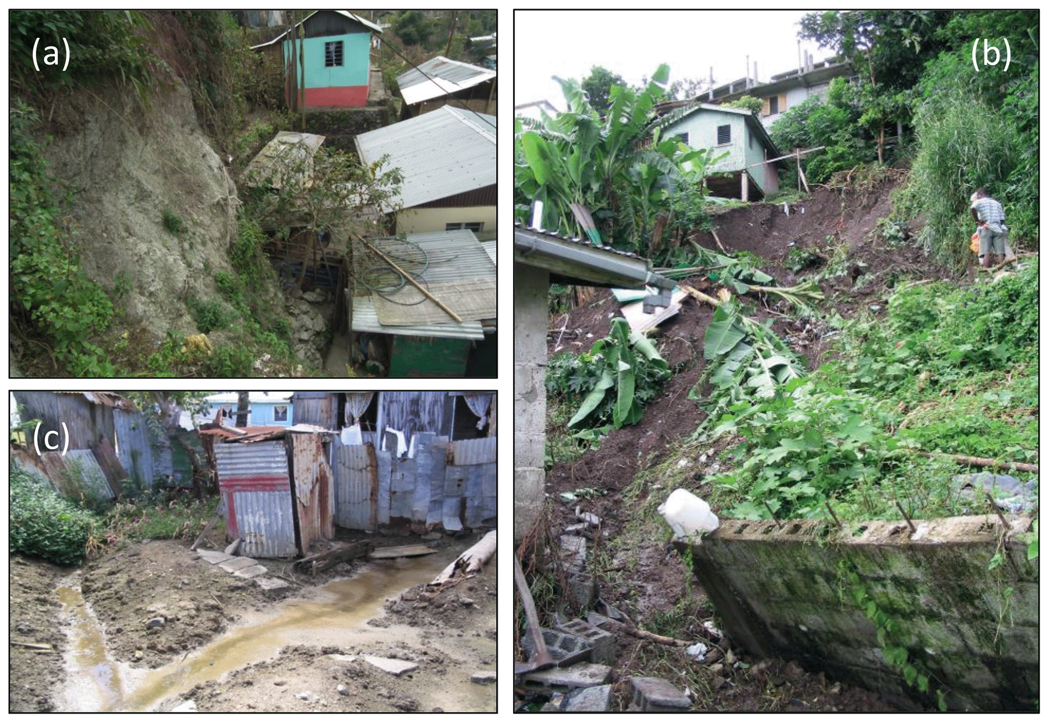
Figure 1Examples of informal housing affecting land stability. Panels (a) and (b) show examples of unsupported cut slopes, respectively, in Dumsi Pakha (Kalimpong, India) and Saint Lucia (Caribbean). Panel (c) shows the effect of the lack of water management in an informal community of Saint Lucia (Caribbean). From the AGU Landslide Blog (https://blogs.agu.org/landslideblog/2016/03/14/managing-urban-landslides-1/, last access: 21 November 2020) and the community-based project Mossaic (Management of Slope Stability In Communities; Anderson and Holcombe, 2013).
However, informal housing is usually neglected or not quantified in landslide hazard assessment at community and larger scales. There are two main reasons for this: lack of reporting and the highly localised scale and heterogeneous nature of human landslide drivers. A landslide is defined as triggered by human activities when there is a direct (and easily recognisable) connection with the failure process (e.g. during mining activities). Landslides of this type are small and often not recorded (Petley, 2012). When considering rainfall-triggered landslides, human landslide drivers are often either not considered or not distinguished from the natural drivers (SafeLand, 2011). Urban construction activities are localised, and even if they contribute to land instability, they remain difficult to observe either in situ (e.g. leaking pipes) or via satellite images. For these reasons, there are numerous site-specific analyses that investigate the influence of urban construction activities for individual slopes with known soil and rainfall trigger characteristics (e.g. Preuth et al., 2010; Zhang et al., 2012), but there are few studies that explore the influence of informal housing more widely for different combinations of human landslide drivers, soils, slope geometry, and rainfall triggers. This limits the transferability of the findings from slope to larger scales, where fewer detailed data are available.
Empirical-statistical and heuristic methods have been used in regional studies to link informal housing to the spatial and temporal occurrence of landslides. For example, precipitation and landslide records have been analysed in relation to lithology and land use change (Meusburger and Alewell, 2008; Gerrard and Gardner, 2006) or in relation to soil type and type of settlement (Smyth and Royle, 2000). Here, most of the recorded landslides were found to be associated with poorly regulated construction techniques, water management, and land degradation. Rainfall thresholds for triggering landslides were observed to depend on the proportion of impervious surfaces (Diaz, 1992). However, these analyses did not enable the differentiation of the relative role of natural and human landslide drivers, precluding the translation of the results into actions at the slope, i.e. engineering, scale (Anderson et al., 2013; Maes et al., 2017).
Mechanistic slope hydrology and stability models can be used to represent the landslide drivers for historical, current, and potential future climate conditions (e.g. Ciabatta et al., 2016; Almeida et al., 2017). If these models included the effect of informal housing, the analysis of different combinations of slope, urban, and climate properties could lead to the assessment of the relative role of natural and urban properties in triggering landslides and to the identification of the conditions at which urban construction activities become most detrimental. This could be useful information for engineers to prioritise slopes that are currently at risk, to identify those at higher risk of being impacted in the future, and to deduce appropriate hazard mitigation or preparedness actions. The inclusion of informal housing in slope stability analysis could also lead to considerations about the reliability of rainfall thresholds for triggering landslides within highly urbanised communities since they might be underestimating the level of the hazard (Mendes et al., 2018).
However, the use of data-intensive mechanistic models can be challenging in data-scarce locations, such as in low-income urban settlements. The more complex the model is, the more data will be required to set its parameters and model forcing and the more uncertainties might be introduced into the analysis. Sources of uncertainties can relate to slope and soil properties, urban features, and a limited understanding of physical processes or future scenarios (epistemic uncertainties; see Beven et al., 2018a, for a review of this issue). Many researchers have assessed the impact of uncertainties related to slope properties (e.g. Cho, 2007) and future climate (e.g. Ciabatta et al., 2016) on slope stability at different scales. However, to the best of our knowledge, there are no analyses that consider both sources of uncertainties when modelling informal housing in landslide hazard assessment. Urban construction activities are considered separately (e.g. slope cutting or leaking pipes; e.g. El-Ramly et al., 2006), or the slope properties are varied using discrete conservative values under fixed rainstorm conditions (Anderson et al., 2008; Holcombe et al., 2016). This separation might overlook significant changes in the slope's behaviour for combinations of urban construction activities and/or combinations of slope, soil, and rainfall properties that have not been considered in the analysis but are still likely to occur.
Almeida et al. (2017) demonstrated how mechanistic landslide models can consider uncertainties due to both poorly defined slope properties and to potential future climate changes. The mechanistic model CHASM (Combined Hydrology and Stability Model) was used in a Monte Carlo framework and applied in Saint Lucia, in the eastern Caribbean, where data support is limited, but landslide hazard is particularly high. The uncertainties in slope and soil properties were characterised through probability distributions extrapolated from available data and the literature, while the rainfall properties were varied uniformly across wide ranges also considering rainfall intensity–duration combinations that were not observed in the past but that might occur in the future. A sample of tens of thousands of rainfall events and slopes were stochastically generated from these distributions and simulated in CHASM. By this approach the possible effects of climate change were explored widely instead of focusing on one (or a few) climate projection scenarios (such as those provided by downscaled generalised circulation models) propagated through the modelling chain (Groves and Lempert, 2007; Wilby and Dessai, 2010). This strategy can be extended to include the exploration of both feasible climate and feasible land use futures (Singh et al., 2014). Statistical and data-mining algorithms were then used by Almeida et al. (2017) to quantify the relative role of the input factors (and thus their uncertainties) in the stability of the simulated slopes as well as to identify critical thresholds in slope properties and rainfall drivers likely to lead to slope failure. In this study we extend the work of Almeida et al. (2017) by including informal housing into such a slope stability analysis. We consider the same location of the humid tropics and the same core model, CHASM, but with new functions to represent the mechanistic influences of informal housing (new CHASM+). The core model is a two-dimensional model which has a relatively low data requirement for a mechanistic model even with the inclusion of the new informal-housing functions. In addition to the original ability to represent the mechanical and hydrological effects of vegetation and the effects of slope cutting and loading, we have added the effects of point water sources resulting from leaking septic tanks, water supply pipes, and houses without roof gutters. By varying both the natural and urban factors, we aim to identify the slope and climate conditions under which landslide hazard is significantly increased by the presence of informal housing and how this information can be used for deducing landslide mitigation measures. Thus, for our humid tropical case study scenario, we aim to address the following questions:
-
How can we identify which informal urban housing characteristics are most detrimental to slope stability?
-
How is the rainfall threshold for triggering landslides modified when informal housing is considered?
-
Which landslide mitigation strategies and practices can be deduced from the analysis for current and potential future scenarios of urbanisation and rainfall?
The proposed methodology is suitable for data-scarce contexts, i.e. when not many field measurements or landslide inventories are available. If applied in countries with similar natural, climate, and urban characteristics (so with similar input space variability), we might expect similar slope stability responses and thresholds. Conversely, a change in (part of) the input data (or their probability distributions) to reflect a different urban-landslide context could potentially produce quite different outputs (Wagener and Pianosi, 2019).
We want to analyse the relative role of informal housing in slope stability under different natural and climate conditions. The methodology we introduce here entails the following steps:
-
Choose a model that represents the main instability mechanisms of the case study area. We are interested in representing the rainfall-triggered landslides and the informal housing of Saint Lucia (Caribbean). We therefore use the mechanistic model CHASM, which represents not only the hydrology-stability routing but also vegetation, slope cutting, and, with the addition of new functions, various forms of water management (creating the extended CHASM+).
-
Define the input factors necessary to run the model and their variability space. In our case study, the input factors are the parameters defining the slope soil, geometry, urban characteristics, and rainfall-forcing data. Each input factor is assumed to be a random variable, and its range of variability is determined by a probability distribution. The probability distributions can be defined based on the physical meaning of the input factors, available data, and/or the existing literature. We use information gathered both from fieldwork in Saint Lucia and also from the literature.
-
Create synthetic combinations of input factors by stochastically sampling from their probability distributions, and run CHASM+ to generate an equivalent number of model outputs. We select the minimum factor of safety (FoS) and the slip surface where the minimum FoS is calculated as summary output variables to analyse. We repeat the stochastic sampling with and without including the urban properties among the input factors in order to facilitate considerations about the role of informal housing in land stability.
-
Identify the input factors that most influence slope stability using global sensitivity analysis (Wagener and Pianosi, 2019). In particular, we use a regional sensitivity analysis (RSA) approach (Hornberger and Spear, 1981) to identify which input factors are most influential in leading to slope failure.
-
Identify parameters' thresholds beyond which the slopes become unstable. The threshold of an input factor over or below which failure is predicted might depend on the value of the other input factors (e.g. slopes with higher slope angles require higher soil strength to maintain stability). Machine learning is a set of methods that computers use to understand trends from data, also considering their mutual interactions. We use CARTs (classification and regression trees) to develop a set of decision rules that predict the combination of soil, geometry, urbanisation, and rainfall input values for which a particular slope is more likely to fail.
In the following paragraphs we describe in detail the tools and the data used to implement our analysis on the island of Saint Lucia.
2.1 The case study: Saint Lucia, eastern Caribbean
Saint Lucia is an eastern Caribbean island with a humid tropical climate. The main landslide trigger is rainfall, and shallow rotational landslides dominate on both steep and shallow slopes (Van Westen, 2016; Anderson and Holcombe, 2013). The geology is almost entirely comprised of volcanic bedrock and deep volcanic deposits. Due to the tropical climate, these volcanic parent materials are subjected to deep weathering, which decreases their strength and increases landslide susceptibility. The strata of a typical slope cross section comprise weathered residual soils overlying decomposed rock and volcanic bedrock. These three types of strata typically correspond, respectively, to the weathering grades V–VI, III–IV, and I–II of the Hong Kong Geotechnical Engineering Office weathering grade classification (GEO, 1988). There is a high variability in terms of engineering soils, but they can broadly be classified as fine-grained soils such as silty clays, clayey silts, and sandy clays (DeGraff, 1985). The combination of tropical climate, steep topography, and volcanic geology renders the region particularly susceptible to rainfall-triggered landslides. Furthermore, landslide risk is increased by informal housing which occupies steep slopes and employs unregulated engineering practices (World Bank, 2012, 226–235). Various sources of information on the slope, soil, rainfall, and urban properties of this region are available from previous studies by government engineers and planners, the local water company, and consultants (e.g. CHARIM, 2015; Mott MacDonald, 2013; Klohn-Crippen, 1995) as well as from community-based projects for the improvement of slope stability with surface water drainage works (Anderson and Holcombe, 2013). In this project, estimates of soil strength properties are based on direct shear tests of local soils (Anderson and Kemp, 1985; DIWI, 2002; Holcombe, 2006) and secondary data sources on similar volcanic tropical residual soils such as those in Hong Kong (Anderson, 1982; Anderson and Howes, 1985). Information about soil type, soil depth, type of house construction, cut slope angles, and the management of surface run-off and waste water on slopes was based on community-based mapping and elicitation of local expert knowledge undertaken by Anderson and Holcombe (2013), who co-developed these datasets with residents, government, and local experts.
2.2 CHASM: a mechanistic model for rainfall-triggered landslides
CHASM (Combined Hydrology and Stability Model) is a 2-D mechanistic model which analyses dynamic slope hydrology and its effect on slope stability over time. A full description of the model can be found in Anderson and Lloyd (1991) and Wilkinson et al. (2002a, b). Here we briefly describe its hydrology and stability components, whereas the representation of the urban properties is detailed in Sect. 2.3. In CHASM the slope cross section is represented with a regular mesh of columns and cells. Hydrological and geotechnical parameters are specified per cell, while the initial hydrological conditions define the position of the water table and the matric suction of the top cell of each column. The dynamic forcing for CHASM is rainfall specified in terms of intensity and duration. For each computational time step (usually 10–60 s), a forward explicit finite-difference method is used to solve the Richard's (1-D, vertical flow) and Darcy's (2-D flow) equations, which regulate, respectively, the unsaturated and saturated groundwater flow. At the end of each simulation hour, the resulting soil pore water pressures (positive and negative) are used as input for the slope stability analysis, which implements Bishop's simplified circular limit equilibrium method (Bishop, 1955) and uses the coordinates of the slope surface. An automated search algorithm identifies the location of the slip surface with the minimum factor of safety, FoS, which is given as output at the end of each simulated hour. In a validation exercise in Hong Kong, CHASM showed an accuracy of 72.5 % (Anderson, 1990), which is comparable to the performances of other models used for the stability analysis (e.g. Formetta et al., 2014, p. 639). CHASM has been employed in Malaysia, Indonesia, eastern Caribbean, and New Zealand to propose landslide mitigation measures as well as to identify land instability drivers along roads and in urban and rural areas (Brooks et al., 2004; Lloyd et al., 2001). Almeida et al. (2017) used CHASM stochastically in a Monte Carlo framework to account for uncertainties in both slope properties and future climate scenarios.
2.3 A new functionality in CHASM: urban point water sources
The new CHASM+ can now represent not only slope cutting, additional (house and tank) load, and vegetation removal but also the presence or absence of roof gutters on houses and localised water leakages from buried septic tanks and superficial water supply pipe networks. Slope cuttings are represented by a corresponding change in slope geometry; additional loads are simulated by appropriately increasing the unit weight of the soil underneath the loading object (i.e. house and tanks); vegetation, which is removed during the urbanisation process, is represented through rainfall interception, evapotranspiration, root water uptake, vegetation surcharge, and increased permeability and soil cohesion due to the root network (see Wilkinson et al., 2002b). Pipes above ground and buried tanks can be added to the slope with specified dimensions and leakage rates. Pipe leakage is accounted for as additional surface water which infiltrates into the slope according to the infiltration capacity of the soil. If water exceeds the infiltration capacity of the soil, it is stored as ponding water. If the ponding water exceeds the maximum water detention capacity (set at 10 mm), the water excess is removed (no run-off considered). Leakage from tanks is added to the water moisture content in the soil cells underneath the tank. Where houses are present, rainfall is intercepted by the roof. If roof gutters are not included, the intercepted rainwater is discharged onto the slope cells adjacent to the house in accordance to the roof type (double- or single-pitch). More details on the new functionality and its benchmarking against another model are given in the Supplement that accompanies this paper (Sect. S1.1 and S1.2).
2.4 Definition of the input factors and their probability distributions
We use 30 input factors to characterise our case study area in CHASM+. These factors fall into the following categories: slope profile geometry, soil geotechnical and hydrological properties, urban characteristics, initial hydrological conditions, and rainfall properties. Table 1 reports the full list of these input factors and the probability distributions that define their range of variability, while Fig. 4 shows an example of a slope derived from a combination of input factors.
Table 1Input factors of CHASM+ and their probability distributions.

U: uniform distribution; Ud: discrete uniform; N: normal distribution; Ln: log-normal distribution. * Layer 1: residual soil, weathering grade V–VI; layer 2: weathered material grade III–IV; layer 3: bedrock grade I–II; weathering grades defined according to GEO (1988). a Effective cohesion > 0. Effective cohesion c (layer 3) > c (layer 2) > c (layer 1). b Effective friction angle > 0. Effective friction angle φ (layer 3) > φ (layer 2) > φ (layer 1). φ<90∘. c , where γs is the saturated unit weight. γd (layer 3) > γd (layer 2) > γd (layer 1). d Values from Hodnett and Tomasella (2002) for sandy clay loam material. We impose n>1; θsat>θres; θres>0. VG: Van Genuchten parameters for defining suction moisture characteristics curve. e Water table height is defined as a percentage of slope height measured to the toe of the slope. f Slope of the cut forced to be between 39 and 89∘, and it is always greater than natural slope angle. g A 0 stands for house without rain gutters; 1 stands for house with rain gutters. Roof type: double pitch. h Vegetation presence: 0 – no vegetation, 1 – insert vegetation in the spare spaces. i The leak of the septic tank is equal to the leak of the pipe. When 0 is selected there is no leak, whilst with 1 there are both. The leak rate is constant and equal to m3 s−1.
The slope geometric properties consist of the natural slope (and associated slope height) and the material thickness. Slope angles vary between 20 and 45∘ to represent typical scenarios of informal housing on moderate and steep slopes. The highest slope angle on which a settlement can be located without some form of engineered slope stabilisation measures is considered to be 45∘. The cross-sectional profile is discretised into three parallel layers of materials to represent the typical weathering profile of volcanic parent material, with a layer of residual soil at the surface (layer 1), underlain by a layer of weathered material (layer 2) and then unweathered bedrock (layer 3). Ranges of material thickness and geotechnical properties are derived from previous fieldwork and lab tests, as described in Sect. 2.1.
The height of the water table is defined as an initial hydrological condition. This water table height is varied between 0 % and 90 % of the slope height (H in Fig. 4) to account for its variability across the region and for the variability in the initial soil moisture conditions due to antecedent rainfall events.
The model is forced with rainfall events which are specified in terms of their duration (in hours) and hourly intensity. The aim is to create both rainfall events that have been observed in the past and rainfall events that might occur in the future (e.g. with higher intensity and duration than observed historically). To constrain the rainfall variability space, we use the intensity–duration–frequency relationships (IDFs) derived from a Gumbel analysis of 40 years of daily rainfall data from weather stations across the island by Klohn–Crippen (1995; Fig. 2). From these IDFs we derive a range of rainfall intensities between 0 and 200 mm h−1 and a range of rainfall durations between 0 and 72 h. We then sample independently from the two uniform distributions, thus obtaining combinations of intensity and duration that might have been observed in the past (light-grey area in Fig. 2) or not (dark-grey area in Fig. 2). Prior to the initiation of the rainfall event we include 168 h (7 d) of simulation with rainfall intensity equal to 0. This ensures a redistribution of water moisture in the unsaturated zone of the slope and allows hydrological equilibrium with steady-state seepage to be established. A further 168 h of zero-rainfall simulation was added after the storm in order to consider the groundwater response after the rainfall event.

Figure 2Rainfall intensity–duration–frequency (IDF) curves for Saint Lucia developed by Klohn–Crippen (1995) using Gumbel analysis of 40 years of daily rainfall data from 15 rainfall gauges. The light-grey section includes rainfall events from observed data (below IDF curves); the dark-grey section represents combinations of rainfall intensity–duration not recorded in the past but that might occur in the future (above IDF curves).
Informal housing is represented by four urban properties: slope cutting, absence of roof gutters, vegetation removal, and leaking pipes and tanks. While the angle of the cut slope is varied according to its probability distribution, the vegetation, roof gutters, and water leakage are defined as present (option 1: yes) or absent (option 0: no; Fig. 3). The cut slope angle is varied between 39 and 89∘, with a maximum cut slope height equal to 4 m. We represent the maximum number of cut slopes that can accommodate a house that is 4 m wide (+1 m of surrounding space) on a slope that is 70 m long. We therefore obtain either five or six cut slopes and a corresponding number of houses on each slope depending on the angle of the cut slope. The house width and house load (8 kN m−2) are not varied and correspond to the size and load of informal houses constructed with shallow concrete strip or block foundations, wooden walls, and sheet-metal roofing that are typically observed in Saint Lucia (Holcombe et al., 2016). When vegetation is present on the original non-urbanised slope, it is removed on the surface of the cuts for the urban scenario. The vegetation properties used represent a tropical forest cover, a sensitive choice for this study site (see Holcombe et al., 2016, and online Supplement, Table S5). These properties are kept fixed throughout the sampling; therefore the effect of different types of vegetation on slope stability is not analysed. Both the tank and the pipe leakage rate are assumed to be half of m3 s−1, which corresponds to the estimated leakage of 15 % of the total water supply for low-income households in Saint Lucia (Anderson and Holcombe, 2013). When present, the leak is kept constant during the simulation time.
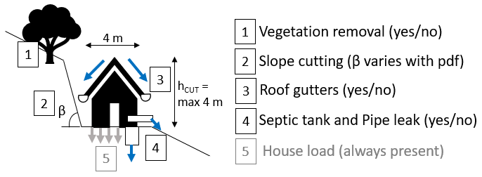
Figure 3Urban properties of informal housing included in the slope stability analysis. Each house corresponds to a cut on the slope. Cut slope angle varies according to its probability distribution, defined in Table 1. Vegetation, roof gutters, and leaking tanks and pipes are stochastically inserted or not. The house on the cut slope is always present, and its load is not varied. The height of the cut slope varies relative to the cut slope angle, but it is forced to be maximum 4 m.
The input factors that define the discretisation of the model, such as the cell size of 1 m × 1 m and the computational time step of 60 s (both used by CHASM+'s dynamic hydrology functions), and the slip search grid location and dimensions are not varied. These values are chosen because they typically ensure numerical stability relating to the mass balance of the moisture in the domain and thus a minimum number of failed model runs. A smaller cell size would enable a more detailed representation of the slope hydrology, but it would require smaller time steps to preserve the moisture content mass balance and numerical stability. Smaller time steps would result in significantly longer simulation time. The resolution chosen is therefore a trade-off between acceptable accuracy and calculation time. The influence of the variation in these two discretisation parameters on slope stability is not explored.
2.5 Creation of synthetic combinations of input factors and model simulation
We use Latin hypercube sampling (McKay et al., 1979) to generate 10 000 different combinations of the 30 independently varying input factors shown in Table 1. Figure 4 illustrates one example of a slope defined by a single combination of these input factors. Due to the randomness of the process, checks are undertaken to ensure that realistic combinations of factors are generated; if not, they are discarded (around 70 % of the time) and replaced by another randomly generated, feasible combination. These “feasibility” checks are reported in the footnote of Table 1 (letters a–f). The stochastically generated simulations are then run in CHASM+ using the high-performance computer BlueCrystal Phase 3 at the University of Bristol. The outputs considered for each simulation are the minimum factor of safety (FoS) and the slip surface where the minimum FoS is calculated. We divide the completed simulations according to whether the minimum FoS is less than 1 (slope predicted to have failed, i.e. a landslide) or greater than 1 (slope is predicted stable). We exclude the simulations predicting that the slope is failed before the start of the rainfall event, which represents inherently unstable slopes (for example steep slopes with deep soil thickness). We repeat the same procedure with and without including the urban properties. We therefore obtain two sets of model outputs: 10 000 representing urbanised slopes and 10 000 representing non-urbanised slopes.
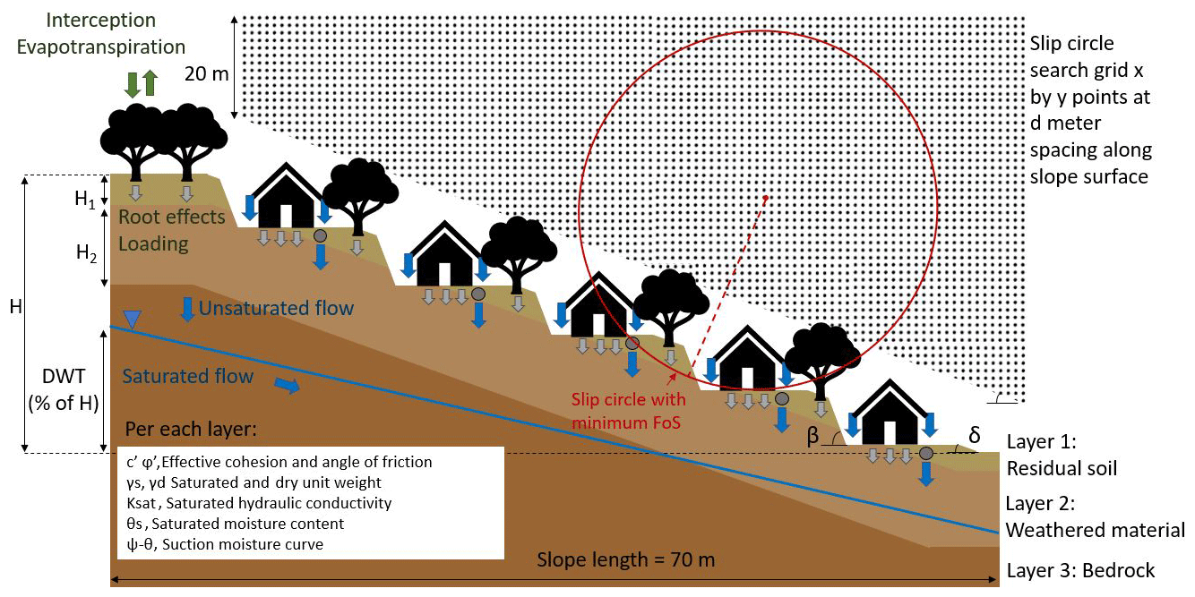
Figure 4Example of slope generated by stochastically sampling from the ranges of input factors specified in Table 1. H is the slope height resulting from the fixed slope length and varying slope angles. The dimensions of the slip circle search grid are fixed, with an initial height of 20 m and width equal to the slope length. The grid extends downslope parallel to the slope as shown.
2.6 Regional sensitivity analysis (RSA) and classification and regression trees (CART)
Global sensitivity analysis is a set of statistical techniques that evaluate how the variations in a model's outputs can be attributed to the variations in the model's input factors. In this case we want to identify which input factors – among geometry, soil, hydrology, rainfall, and urban properties – have the strongest impact on slope stability. Since in our case the model output is binary as simulated slopes are categorised as failed (if FoS < 1) or stable (FoS > 1), we use the regional sensitivity analysis (RSA) approach (Hornberger and Spear, 1981), which is particularly suitable when dealing with categorical outputs. In the RSA approach, the cumulative marginal distribution of each input factor is computed for each output category, i.e. the stable slopes and the failed ones. If the distributions significantly separate out, it is taken as evidence that the model output (slope stability) is significantly affected by variations in the considered input factor. The level of separation between the cumulative distributions can be formally measured with the Kolmorov–Smirnov (KS) statistic and used as a sensitivity index. The confidence intervals of the sensitivity indices can be estimated via bootstrap technique. The bootstrap randomly draws N samples (with replacement) from the available data to compute N KS statistics for each input factor. The magnitude of fluctuations in the KS statistic from one sample to another represents the level of confidence in the estimation of the sensitivity indices. For this application, we use the SAFE (Sensitivity Analysis For Everybody) toolbox (Pianosi et al., 2015) to perform RSA and to calculate the sensitivity indices and their confidence intervals by the bootstrapping technique.
Classification and regression tree (CART) analysis is a supervised machine learning method which we use to predict critical thresholds in input factors over or below which a particular slope is more likely to fail (Breiman et al., 1984). In this analysis, the predictor model takes the form of a binary tree. Starting from the whole set of simulations, CART finds the best possible input factor (e.g. slope angle rather than rainfall intensity) and the best possible value of that input factor (e.g. slope angle greater or less than 30∘) that divide the simulations into stable and failed simulations. This process is recursively repeated, creating at every split two branches and two (“child”) nodes of the tree. In choosing the best splitter, the model seeks to maximise the “purity”, i.e. to maximise the number of stable or failed simulations at the two generated nodes. Amongst the different measures of purity available, we use the Gini purity index defined as
where m is the number of categories for the output (in this case two: stable or failed), and p(i) is the fraction of simulations in the node belonging to category i. The Gini purity index is 0 when all the simulations in the considered node belong to the same category (a “pure” node, i.e. all stable or failed). The splitting process typically continues until all final leaf nodes show Gini purity indices below a chosen threshold. The final nodes express the prediction for the corresponding branch. While a high number of nodes increases predicting accuracy, it also makes the model more difficult to interpret and generalise to other datasets (i.e. the problem of overfitting). A pruning technique can be applied to avoid this overfitting and to identify an acceptable trade-off between predictive power and number of nodes. In this analysis, we build a CART within the MATLAB Statistics and Machine Learning Toolbox (Mathworks, 2018) using the K-fold cross-validation to better estimate its predictive power. In particular, we use 10-fold cross-validation, which randomly divides the original dataset (10 000 simulations) into 10 subgroups. A total of nine subgroups are used to construct 10 CARTs, while the remaining subgroup is used to test the CARTs' performance. The average value of the 10 misclassification errors so obtained represents the cross-validation error, which can be used to select suitable pruning levels. To reduce the number of nodes without increasing the misclassification errors, auxiliary variables can be used to combine correlated input factors. Auxiliary variables can simplify the tree's structure (by using fewer combined input factors) and potentially modify the input space in a way that the division of failed and stable simulations is more effective (see rotation of the coordinate systems in Dalal et al., 2013). Three auxiliary variables are used in this analysis: the ratio of soil thickness and effective soil cohesion of layer 1, the ratio between rainfall intensity and duration introduced (both introduced by Almeida et al., 2017), and a weighted combination of natural and cut slopes angles. These variables are described in the results (CART analysis) section and Sect. S2.
In this section we analyse the 10 000×2 outputs generated by CHASM+ for the urbanised and non-urbanised slope scenarios. As previously mentioned, we split the simulations into stable and failed according to the value of the minimum FoS (respectively, greater or less than 1). As a first analysis we compare the percentage of failed slopes against stable slopes for each of the urban properties. Figure 5 shows that the presence of cut slopes significantly influences the percentage of predicted slope failures: the steeper the cut slope angle, the higher the percentage of failed slopes. Vegetation removal and roof gutters instead have a negligible role in dividing the two sets. Last, septic tanks and leaking pipes have some effect, generating about 10 % more failed slopes when present.
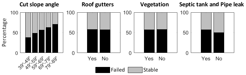
Figure 5Percentage of predicted stable and failed slopes per urban property. An urban property influences slope stability if the percentage of the predicted failures changes with the variation in that urban property.
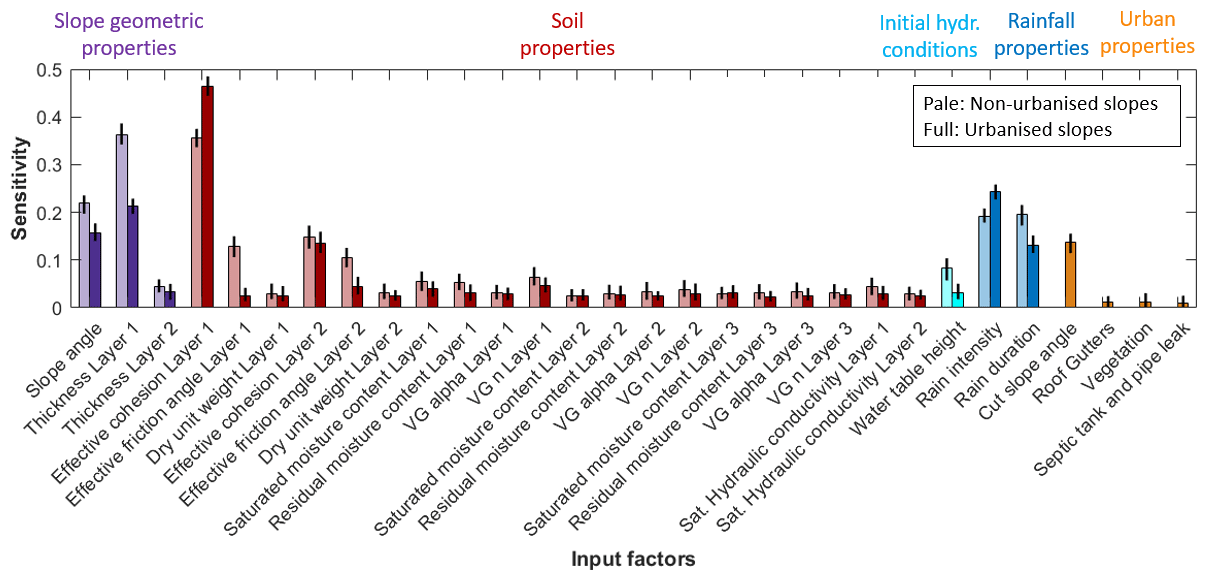
Figure 6Sensitivity index for each input factor in the urbanised (full colour) and non-urbanised (pale colour) cases. The bars correspond to the mean value of sensitivity for each input factor calculated with bootstrapping, while the vertical black lines at the top of the bars represent the confidence interval (number of bootstrap resampling N=100; significance level for the confidence intervals: 0.05).
3.1 Regional sensitivity analysis
We then perform RSA on both sets of urbanised and non-urbanised slope simulations, calculating the cumulative marginal distributions of the failed and stable simulations for each input factor. The maximum distance between the two distributions (KS statistic) is computed and used as a sensitivity index. A high value of the sensitivity index suggests that the variation in that input factor significantly influences slope stability. The results are shown in Fig. 6 for both urbanised and non-urbanised slopes. Figure 6 shows that slope stability is insensitive to many input factors and highly sensitive to few, namely effective cohesion and thickness of layer 1 (residual soil), slope angle, and rain intensity and duration. These sensitive input factors represent the main landslide drivers. The sensitivity indices of the urban properties (in orange) are consistent with the findings of Fig. 5, where only the variation in cut slope angle influences slope stability. When looking at the comparison between urbanised and non-urbanised slopes, it appears that the urban presence decreases the sensitivity indices of all the input factors, except for the effective cohesion of layer 1 and the rainfall intensity.
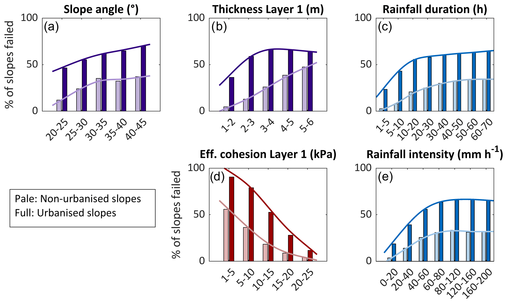
Figure 7Percentage of slope failures for urbanised and non-urbanised slopes for different categories of input factors. Throughout, urbanised slopes show higher failure rates than non-urbanised slopes. In (a–c) the distribution of failure rates for urbanised slopes is more uniform for variations in input factors than the non-urbanised case, while in (d, e) it is more pronounced. Panels (a–c) represent the input factors whose sensitivity indices are smaller when urbanisation is introduced in Fig. 6, while (d, e) show the input factors whose sensitivity gets larger when urbanisation is introduced in Fig. 6.
We further explore the change in sensitivity caused by urbanisation by plotting the percentage of failed slopes for the main landslide drivers (Fig. 7). The figure shows how this percentage varies for the urbanised (full colour bars and lines) and non-urbanised cases (pale colour bars and lines). In general, urbanised slopes produce more failures than non-urbanised slopes, though they both display similar trends: an increased percentage of predicted landslides when we would expect the slope to become more susceptible (e.g. when slope angles are higher) or the trigger more severe (when rainfall intensity and duration are larger). For example, in Fig. 7b the percentage of failed slopes in the non-urbanised case linearly increases from ∼5 % (for soil thickness 1–2 m) to ∼50 % (thickness of 5–6 m). In the same figure, urbanised slopes show higher failure rates for all values, though the greatest increase occurs for soil thicknesses less than 4 m (up to +46 % for the 2–3 m category). This means that the most significant increase in number of landslides occurs for thin soil thicknesses, i.e. on slopes less susceptible to failure when non-urbanised. The same can be said for slope angles less than 25∘ and rainfall duration less than 10 h, where percentages of slope failures pass from less than 15 % to more than 40 % when urbanisation is introduced (Fig. 7a and c). In the lower plots instead, more urban landslides are observed on slopes that show high percentage of failures also when urbanisation is not present (+43 % for low values of soil cohesion; Fig. 7d; +35 % for high rainfall intensities; Fig. 7e). The difference in failure rates with variations in input factors also explains the change in sensitivity found in Fig. 6: when urbanised, a slope's response varies less (less sensitive) to variations in the input factors in the upper plots (whose sensitivity indices get smaller) and more (more sensitive) to variations in the input factors of the lower plots (whose sensitivity indices get larger).
3.2 CART analysis
We use the CART analysis to formalise the critical thresholds of input factors above or below which slopes are most likely to be predicted as stable or failed. Figure 8 represents the two trees for the non-urbanised (Fig. 8a) and urbanised case (Fig. 8b). As expected, the best predictors selected in CART are the same input factors previously identified as most influential (Fig. 6). The boxes with double colour represent the auxiliary variables that combine correlated input factors: the ratio between effective cohesion and thickness of layer 1 to account for their counterbalancing effect on slope stability (i.e. slope with more cohesive soil can be thicker without experiencing failure); the negative ratio between the logarithm of rainfall intensity and rainfall duration, which represent the slope of the rainfall threshold for triggering landslides; and the weighted average of the natural and the cut slope angles to account for the fact that slope susceptibility can significantly increase for low natural slope angles but high cut slopes angles (see Sect. S2 for details about the auxiliary variables and the change in the model's performance when they are not considered). Using these few predictors, both trees correctly classify more than 85 % of the simulations as stable or failed (details about the pruning in Sect. S3). Each branch of the tree shows the paths and thresholds of input factors that lead to slopes most likely to fail (black branch) or most likely to not fail (grey branch). At the end of each branch the black and grey bar shows the fraction of failed and stable simulations, while the thickness of the branch is proportional to the number of simulations following that path. For example, in the tree resulting from non-urbanised slopes (left-hand side), the thickest grey line shows that more than 50 % of simulated slopes were stable 91.2 % of the time for cohesion ∕ thickness of layer 1 ratios greater than 2.5 kPa m−1. The thick black branch instead shows that the greatest proportion of simulations predicted as failed occurred for cohesion ∕ thickness of layer 1 ratios less than 2.5 kPa m−1, rainfall intensity duration ratios () greater than 0.9 m h−2, and slope angles greater than 25∘.
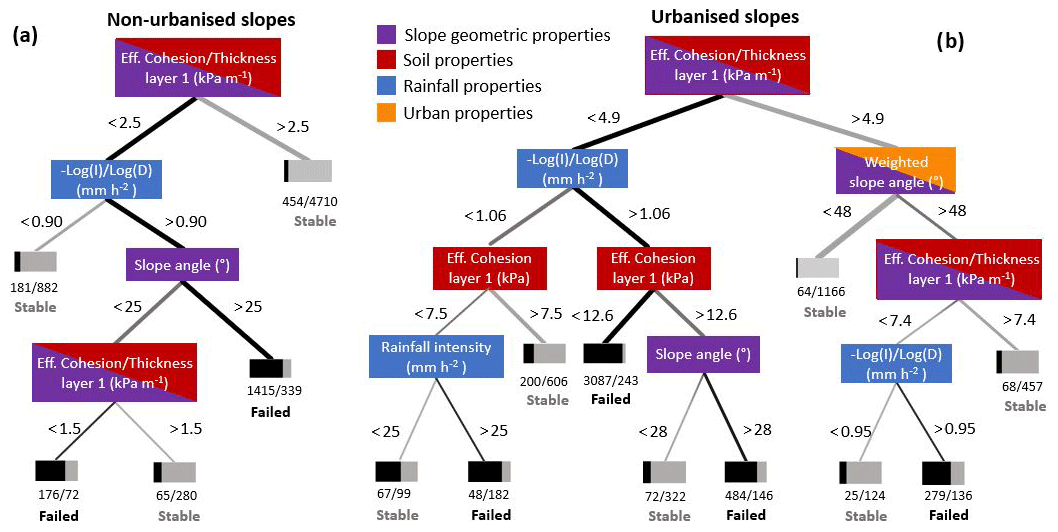
Figure 8Classification tree of slope response for non-urbanised slopes (a) and urbanised slopes (b). Black branches represent the paths that lead to simulations predicted as failed, while grey branches lead to simulations predicted as stable. The bar under each leaf shows the proportion of simulations that were failed (black) or stable (grey) for that leaf. The thickness of the branch is proportional to the number of simulations following that path. Note that 14 % and 22 % of the simulated slopes have been excluded, respectively, for the non-urbanised and urbanised case because they failed before the start of the precipitation.
In the trees resulting from non-urbanised slopes (right-hand side), the black branch leading to the majority of failures is similar to the non-urbanised tree, but it presents higher splitting thresholds: from the top, the split happens for cohesion ∕ thickness of layer 1 ratios less than 4.9 (instead of 2.5) and for a rainfall intensity ∕ duration ratio of 1.06 (instead of 0.9). The branch then leads to the majority of failures for values of effective cohesion of layer 1 less than 12.6 kPa, regardless of the natural slope angle. A higher threshold in cohesion ∕ thickness ratios indicates that when urbanisation is present, more failures occur on slopes with higher soil cohesion and/or thinner soil layers than non-urbanised slopes (compatible with Fig. 7b and d), while higher rainfall intensity duration ratios suggest that more failures occur for higher rainfall intensity and/or lower rainfall durations when compared to non-urbanised slopes (as shown in Fig. 7c and e). Finally, going back to the top and looking at the thick grey branch of the urbanised tree, it can be noted that a ratio between the effective cohesion and the thickness of layer 1 greater than 4.9 ensured 95 % of slope stability only when the weighted slope angle is less than 48∘.
4.1 Slope cutting is the urban construction activity most detrimental to slope stability
In this analysis, slope cutting is the urban construction activity with the strongest effect on slope stability's response (Figs. 5 and 6). Figure 7 indicates that when urbanisation is present, more slope failures are observed, mainly on slopes with relatively low slope angles and with low values of both soil (layer 1) thickness and cohesion (Fig. 7b and d; also reflected by higher effective cohesion ∕ thickness ratios in CART in Fig. 8b). This is interpreted as being caused by cut slopes: when cut slope angles are steep, a higher effective cohesion and thus a higher soil strength are required to maintain stability, regardless of the natural slope angles; when soil layers intersect the cuts, low soil strength is not sufficient to ensure slope stability even on thin – and therefore less landslide-prone – soil layers. The interaction between the depth of soil layer 1 and the cut slope geometry is deduced from Fig. 7b: almost 50 % more failures are observed for a thickness of layer 1 smaller than the slope's height (4 m), i.e. when the interface of soil (layer 1) and weathered material (layer 2) outcrops in the cut slope face (as illustrated in Fig. 4). For these slopes, visual inspection reveals that the slip surface is generally located between layer 1 (residual soil, weathering grade V–VI) and layer 2 (weathered material, grade III–IV). This is explained by the different soil strength of the two layers, which constrains the slip surface within the weaker layer 1, and the different hydraulic conductivities. As rainfall infiltrates, the lower hydraulic conductivity of the underlying weathered material leads to a progressive accumulation of water, promoting a perched water table. The raised pore water pressure decreases the effective soil strength and consequently the stability of the soil layer. Part of the increase in pore water pressure might be caused by the presence of water leakages at the top of the cut slope. However, the low sensitivity of the slope response to leakage (Fig. 6) does not allow for more considerations.
Slope cutting is therefore considered in this analysis to be the practice most detrimental to slope stability. This result is consistent with studies carried out in the humid tropics at regional scales, for which slope cutting was identified as one of the major causes of landslides (e.g. Brand et al., 1984; Froude and Petley, 2018; Holcombe et al., 2016). Cuts with slope angles greater than 60∘ are also considered to be at particularly high risk (e.g. Cheng, 2009), while excess of pore water pressure was shown to be a dominant process in triggering shallow failures on cut slopes (Anderson, 1983). CHASM+ therefore successfully captures these physical mechanisms, confirming, despite the uncertainties, the governing role of soil properties and soil thickness in determining slope equilibrium. The other urban construction activities considered seem to have a less significant role on landslide hazard. Previous studies found that vegetation can be both beneficial and detrimental to slope stability (Wu et al., 1979; Collison et al., 1995). Here we find that its effect is negligible, probably due to its limited presence in urbanised slopes (trees are left at the crest of each cut slope, where they add loading and may actually be detrimental to the local cut slope stability). Also, adding roof gutters does not seem to decrease the number of failed slopes. However, in the scenarios generated here we have only reached a maximum of 30 % slope coverage by houses, i.e. about 30 % of impervious surface (five to six households on 70 m slope) due to our inclusion of cut slopes for every house. Evidence shows that roof guttering effectiveness becomes evident only when the house coverage is above 50 %, and thus a considerable portion of rain does not infiltrate into the slope (Anderson and Holcombe, 2013). On the other hand, leaks from septic tanks and pipes lead to 10 % more failures despite the low house coverage. When higher house densities are considered, the lack of water management might become even more significant (Di Martire et al., 2012).
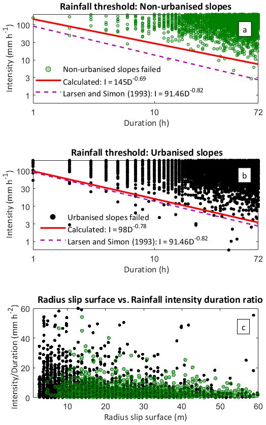
Figure 9In (a) and (b) the red line represents the minimum rainfall thresholds calculated from our stochastic sample (99.9 % of the failed slopes in the sample are above the thresholds). Panel (c) represents the radius of the slip surfaces of the recorded landslides plotted against the corresponding triggering rainfall intensity ∕ duration ratio. Note as in (a) and (b) the x and y axis are in logarithmic base 10 scale, but the notation is linear for easier readability.
4.2 The rainfall threshold for triggering landslides is lower when informal housing is included
We found that when slopes are urbanised, the most significant increase in the percentage of failed slopes occurs for rainstorm events with high intensity (>20 mm h−1) and low duration (<20 h; Fig. 7c and e). Accordingly, our CART analysis identifies a higher threshold of rainfall intensity ∕ duration ratio to divide the stable and failed slopes in the urbanised case (Fig. 8b). In landslide analysis, so-called minimum rainfall thresholds are defined as the combinations of rainfall intensity (I) and duration (D) above which we would expect landslides to start occurring. These thresholds are generally expressed by a power law relationship I=γDα (Guzzetti et al., 2007), and they are constructed based on inventories of observed landslides and the rainfall that triggered them (e.g. Caine, 1980; Larsen and Simon, 1993; Guzzetti et al., 2007). Many countries in the humid tropics have limited empirical data on landslides, and therefore it would be useful to be able to generate such thresholds from stochastic analyses of the type we performed here. To demonstrate how this could be done, we applied a multi-objective optimisation method to our sample of stochastically generated slopes (details about our approach in Sect. S4). We do not use the more commonly employed frequentist methods (Brunetti et al., 2010; Melillo et al., 2018) because the high frequency of failed slopes for high-intensity and long-duration events would strongly bias the position of the threshold. Figure 9a and b show the calculated thresholds on a log–log scale, respectively, for the non-urbanised and urbanised case (red lines). In both cases, 99.9 % of the failed simulations fall above them. The thresholds present the typical descending trend found in empirical analysis, for which lower rainfall intensities are needed to trigger a landslide when rainfall durations increase. The fact that this trend can be replicated by our synthetic simulations indicates that CHASM+ and our stochastic modelling framework are giving realistic hydrological and stability responses to the rainfall forcing.
The higher the intensity and/or the duration of the rainfall event is, the more slope failures will occur in both cases. However, when informal housing is present, more failures are observed for rainfall durations less than 10 h (short events; Larsen and Simon, 1993). This pushes down the intercept of the rainfall threshold, as reflected in the change in the coefficients of the power law equations (reported in each figure). The slope of the threshold line (i.e. the exponent of the power law) is also steeper in the urbanised case, implying the presence of more failures for lower rainfall intensities throughout the duration axis. These results are compatible with the increase in small-scale landslides previously commented (failure depths less than cut slope's height): to reach saturation at shallow depths, relatively low rainfall intensities and durations can be sufficient to initiate slope failure. Figure 9c confirms this assumption: when slopes are urbanised (black dots), failures tend to occur with smaller radius of slip surface and for higher values of intensity ∕ duration ratio. The findings reflect the empirical evidence in low-income communities which report a high frequency of small-scale landslides, particularly associated with cut slopes, for high-intensity and short-duration events (“the everyday disasters”; Bull-Kamanga et al., 2003). Finally, we compare our results with the empirical rainfall threshold proposed by Larsen and Simon (1993) for Puerto Rico, which is based on landslide inventories that also include failures observed on slopes modified by construction activities (mainly slope cuts for road network; see Larsen and Parks, 1997). When informal urbanisation is considered, the two thresholds are almost overlapping (Fig. 9b). This reinforces both the potential of using mechanistic models within a stochastic framework to generate synthetic thresholds in data-scarce locations and the possibility of using the resulting thresholds for regions of the humid tropics with similar geophysical, climatic, and urban properties.
4.3 Guidelines for landslide mitigation actions to tackle the main instability drivers
The identification of the main instability drivers and their thresholds can contribute to create objective rules to classify slopes as hazardous in a region with scarce data availability. For example, in Saint Lucia our analysis suggests that slopes with effective cohesion of layer 1 less than 12 kPa and thickness less than 2.5 m (effective cohesion ∕ thickness of layer 1<4.9) are particularly at risk for rainfall events with intensity ∕ duration ratios greater than 1.06 m h−2 (Fig. 8b). These rules can shape look-up tables or priority ranking to classify human-made slopes as dangerous (Anderson and Lloyd, 1991; Cheng, 2009). Figure 6 shows that only few input factors particularly influence slope stability with or without urbanisation. These are effective cohesion and thickness of the layer 1 (residual soil), natural slope angles, and rain intensity and duration. The crucial role of these factors in regulating slope stability is broadly recognised (Guzzetti et al., 2007; van Westen et al., 2006). The results presented here demonstrate how the influence of these instability drivers can be ranked and quantified. The other input factors might have a smaller direct or indirect effect, but they are not dominant. This is an expected finding in global sensitivity analysis (Wagener and Pianosi, 2019), even if different outputs (e.g. the timing of the failure) might be sensitive to different input factors (e.g. variations in the moisture suction curves, as demonstrated in Sect. S1.2). The identification of these main landslide drivers helps to address data acquisition efforts, while the comparison between urbanised and non-urbanised simulations quantifies the different relative role (e.g. weight) of preparatory factors in landslide susceptibility assessment when informal urbanisation is present. For example, a weighted average of natural and cut slope angle can be used to identify areas (not) at risk.
All the results presented are subjected to the assumptions made in our study. The large variation in some of the input factors can lead to overestimating the hazard. Almeida et al. (2017), for example, varied the slope angles between 27 and 30∘ (instead of between 20 and 45∘) and hence found a lower value of the cohesion ∕ thickness ratio to separate stable and failed slopes than we found (in the non-urbanised case). Data acquisition can help to reduce these uncertainties. However, when data are not available, our approach allows for the identification of so-called “low regrets” mitigation measures, i.e. actions that have a positive impact on slope stability regardless of the uncertain factors. According to our analysis, the most effective action would be avoiding slope cutting since it was shown to be the urban construction activity most detrimental to slope stability. However, this is of scarce utility since informal housing often outstrips urban regulations (Fekade, 2000). Better hazard awareness and construction practices should therefore be suggested. These include for example reducing surface water infiltration on slopes, especially when the topsoil layers intersect the cut slope, and the resulting perched water tables reduce shear strength in a critical location. Slope surface and subsurface drainage can be designed to reduce the infiltration of rainwater to a level that, in effect, reduces the total rainfall intensity below the rainfall threshold calculated. Another cost-effective landslide mitigation strategy can be the planting of deep-rooting grasses, shrubs, or small trees, which increases slope strength (e.g. soil cohesion) in the top couple of metres of soil and also reduces soil moisture content though root water uptake and evapotranspiration (Holcombe et al., 2016; Ng et al., 2011; Wilkinson et al., 2002a, b).
Finally, Fig. 9b shows that when slopes are urbanised, high-intensity, short-duration rainfall events lead to an increased number of small-scale landslides (failure depths less than 4 m; Fig. 7b; and radius of slip failure less than 10 m; Fig. 9c). Future climate change could potentially increase the frequency of intense precipitation events (e.g. O'Gorman and Schneider, 2009) and therefore the occurrence of these types of landslides in informal communities. However, if small-scale failures produced by anthropogenic factors are neglected in the calculation of rainfall thresholds, current rainstorms events could also be excluded as triggering factors (Crozier, 2010; Mendes et al., 2018). Small-scale, high-frequency landslide events might not lead to major disasters, but they are increasingly seen as indicators of risk accumulation, detrimental to disaster resilience and economic development (Bull-Kamanga et al., 2003). For this reason, these types of landslides deserve greater attention from the scientific community.
We include informal housing into slope stability analysis using a newly extended version of the mechanistic model CHASM in a Monte Carlo framework. In this way, we consider uncertainties due to both poorly known slope properties and potential future changes in urban and climate conditions. We demonstrate that informal housing increases landslide hazard and that slope cutting is the most detrimental construction activity when compared to vegetation removal, lack of roof gutters, and presence of water leaks. The presence of informal housing also modifies the relative role that natural slope angle, soil cohesion, and soil thickness have in maintaining stable slopes, with increased hazard occurrence for low values of these three main landslide drivers. CART analysis identifies the thresholds of input factors separating stable and unstable slopes. These thresholds can be used as objective criteria for guiding local engineers in identifying slopes at risk, deducing landslide mitigation actions, and targeting data acquisition to reduce model prediction uncertainty. Moreover, this analysis allows for the estimation of critical rainfall thresholds at which slope failure is predicted to occur. This rainfall threshold is lower when informal housing is present, with an increased number of small-scale landslides (+85 %, with failure depth less than 4 m and radius of slip surface less than 10 m) for high-intensity and short-duration events. The rainfall threshold resulting from the urbanised slopes is comparable to the one proposed by Larsen and Simon (1993) for the region of Puerto Rico, suggesting its potential validity also for other similar (data-scarce) regions of the humid tropics.
Future work will seek to vary the properties that were kept constant in this study, such as the degree of urbanisation and house dimensions, to evaluate their significance for slope stability. This might confirm the importance of household water management such as roof guttering and leaking water supply pipes and septic tanks when the number of households is increased. Analysis of slopes where slope cutting is replaced by other possible construction techniques (such as houses suspended on pile foundations) can identify whether the construction of future hillside settlements could be done in a manner less detrimental to slope stability. Different bioengineering techniques to mitigate hazard likelihood could also be modelled and their effectiveness evaluated. Finally, we seek to transfer the thresholds found in our CART analysis into spatial-scale susceptibility maps in order to identify slopes at higher risk within low-income urban settlements. This would confirm whether the areas suggested to be most hazardous correspond to areas where more landslides have been observed.
Datasets can be accessed by reviewing the data sources stated in Sects. 2.1 and 2.4.
The supplement related to this article is available online at: https://doi.org/10.5194/nhess-20-3161-2020-supplement.
EB performed background research, computations, and analysis and wrote the paper. EH, FP, and TW supervised the entire study in all stages, discussed the results, and contributed to the final paper.
The authors declare that they have no conflict of interest.
Existing MATLAB codes from Susana Almeida and Rose Hen-Jones have been adapted and extended for this analysis. We thank Dave Petley (University of Sheffield) for giving permission to use one of the pictures for Kalimpong, India (https://blogs.agu.org/landslideblog/2016/03/14/managing-urban-landslides-1/, last access: 21 November 2020).
The first author was supported by an EPSRC DTP studentship (grant no. EP/N509619/1). Partial support to Thorsten Wagener was provided by a Royal Society Wolfson Research Merit Award (WM170042). Francesca Pianosi is partially funded by the Engineering and Physical Sciences Research Council (EPSRC) “Living with Environmental Uncertainty” Fellowship (EP/R007330/1).
This paper was edited by Margreth Keiler and reviewed by two anonymous referees.
Almeida, S., Ann Holcombe, E., Pianosi, F., and Wagener, T.: Dealing with deep uncertainties in landslide modelling for disaster risk reduction under climate change, Nat. Hazards Earth Syst. Sci., 17, 225–241, https://doi.org/10.5194/nhess-17-225-2017, 2017.
Anderson, M., Holcombe, L., Flory, R., and Renaud, J. P.: Implementing low-cost landslide risk reduction: A pilot study in unplanned housing areas of the Caribbean, Nat. Hazards, 47, 297–315, https://doi.org/10.1007/s11069-008-9220-z, 2008.
Anderson, M. G.: Mid-Levels Study. Report on Geology, Hydrology and Soil Properties, Geotechnical Control Office, Civil Engineering Services Department, Hong Kong, 1982.
Anderson, M. G.: Road-cut slope topography and stability relationships in St Lucia, West Indies, Appl. Geogr., 3, 105–114, https://doi.org/10.1016/0143-6228(83)90033-4, 1983.
Anderson, M. G.: A feasibility study in mathematical modelling of slope hydrology and stability, Report, Geotechnical Control Office Civil Engineering Services Department, Hong Kong, 1990.
Anderson, M. G. and Holcombe, E.: Community-based landslide risk reduction: managing disasters in small steps, World Bank, Washington, D.C., available at: https://openknowledge.worldbank.org/handle/10986/12239 (last access: 24 November 2020), 2013.
Anderson, M. G. and Howes, S.: Development and application of a combined soil water-slope stability model, Q. J. Eng. Geol. Hydrogeol., 18, 225–236, 1985.
Anderson, M. G. and Kemp, M. J.: The prediction of pore water pressure conditions in road cut slopes, St Lucia, West Indies, Final Technical Report R3426, Overseas Development Agency, London, UK, 1985.
Anderson, M. G. and Lloyd, D. M.: Using A Combined Slope Hydrology–Stability Model To Develop Cut Slope Design Charts, Proc. Inst. Civ. Eng., 91, 705–718, 1991.
Anderson, M. G., Holcombe, E., Holm-Nielsen, N., and Della Monica, R.: What Are the Emerging Challenges for Community-Based Landslide Risk Reduction in Developing Countries?, Nat. Hazards Rev., 15, 128–139, https://doi.org/10.1061/(asce)nh.1527-6996.0000125, 2013.
Beven, K. J., Almeida, S., Aspinall, W. P., Bates, P. D., Blazkova, S., Borgomeo, E., Freer, J., Goda, K., Hall, J. W., Phillips, J. C., Simpson, M., Smith, P. J., Stephenson, D. B., Wagener, T., Watson, M., and Wilkins, K. L.: Epistemic uncertainties and natural hazard risk assessment – Part 1: A review of different natural hazard areas, Nat. Hazards Earth Syst. Sci., 18, 2741–2768, https://doi.org/10.5194/nhess-18-2741-2018, 2018a.
Bishop, A. W.: The use of the Slip Circle in the Stability Analysis of Slopes, Géotechnique, 5, 7–17, https://doi.org/10.1680/geot.1955.5.1.7, 1955.
Brand, E. W., Premchitt, J., and Phillipson, H. B.: Relationship between rainfall and landslides in Hong Kong, in: vol. 1, Proceedings of the 4th International Symposium on Landslides, September 1984, Canadian Geotechnical Society, Toronto, 377–384, 1984.
Breiman, L., Friedman, J., Stone, C. J., and Olshen, R. A.: Classification and regression trees, CRC Press, Wadsworth and Brooks/Cole Advanced Books and Software, Monterey, CA, 1984.
Brooks, S. M., Crozier, M. J., Glade, T. W., and Anderson, M. G.: Towards Establishing Climatic Thresholds for Slope Instability: Use of a Physically-based Combined Soil Hydrology-slope Stability Model, Pure Appl. Geophys., 161, 881–905, https://doi.org/10.1007/s00024-003-2477-y, 2004.
Brunetti, M. T., Peruccacci, S., Rossi, M., Luciani, S., Valigi, D., and Guzzetti, F.: Rainfall thresholds for the possible occurrence of landslides in Italy, Nat. Hazards Earth Syst. Sci., 10, 447–458, https://doi.org/10.5194/nhess-10-447-2010, 2010.
Bull-Kamanga, L., Diagne, K., Lavell, A., Leon, E., Lerise, F., MacGregor, H., Maskrey, A., Meshack, M., Pelling, M., Reid, H., Satterthwaite, D., Songsore, J., Westgate, K., and Yitambe, A.: From everyday hazards to disasters: the accumulation of risk in urban areas, Environ. Urban., 15, 193–204, 2003.
Caine, N.: The rainfall intensity-duration control of shallow landslides and debris flows, Geogr. Ann. A, 62, 23–27, 1980.
CHARIM: Caribbean Handbook on Risk Information Management, available at: http://www.charim.net/ (last access: 21 November 2020), 2015.
Cheng, P. F. K.: The New Priority Ranking Systems for Man-made Slopes and Retaining Walls, Special Project Report (SPR) 4/2009, Geotech. Eng. Off. (GEO), Hong Kong, 6–14, 2009.
Cho, S. E.: Effects of spatial variability of soil properties on slope stability, Eng. Geol., 92, 97–109, https://doi.org/10.1016/j.enggeo.2007.03.006, 2007.
Ciabatta, L., Camici, S., Brocca, L., Ponziani, F., Stelluti, M., Berni, N., and Moramarco, T.: Assessing the impact of climate-change scenarios on landslide occurrence in Umbria Region, Italy, J. Hydrol., 541, 285–295, https://doi.org/10.1016/j.jhydrol.2016.02.007, 2016.
Collison, A. J. C., Anderson, M. G., and Lloyd, D. M.: Impact of vegetation on slope stability in a humid tropical environment: A modelling approach, Proc. Inst. Civ. Eng. Water, Marit. Energ., 112, 168–175, https://doi.org/10.1680/iwtme.1995.27662, 1995.
Crozier, M. J.: Geomorphology Deciphering the effect of climate change on landslide activity: A review, Geomorphology, 124, 260–267, https://doi.org/10.1016/j.geomorph.2010.04.009, 2010.
Dalal, S., Han, B., Lempert, R., Jaycocks, A., and Hackbarth, A.: Improving scenario discovery using orthogonal rotations, Environ. Model. Softw., 48, 49–64, 2013.
DeGraff, J. F.: Landslide hazard on St. Lucia, West Indies, Final Report, Organization of American States, Washington, D. C., 1985.
Diaz, V. J.: Landslides in the squatter settlements of Caracas; towards a better understanding of causative factors, Environ. Urban., 4, 80–89, 1992.
Di Martire, D., De Rosa, M., Pesce, V., Santangelo, M. A., and Calcaterra, D.: Landslide hazard and land management in high-density urban areas of Campania region, Italy, Nat. Hazards Earth Syst. Sci., 12, 905–926, https://doi.org/10.5194/nhess-12-905-2012, 2012.
DIWI Consult: Materials Report, RDP-001 Soufriere-Choiseul, DIWI Consult International GmbH, Consulting Services for the Roads Development Programme, Ministry of Communications, Works, Transport & Public Utilities, Government of Saint Lucia, unpublished, 2002.
El-Ramly, H., Morgenstern, N. R., and Cruden, D. M.: Probabilistic assessment of stability of a cut slope in residual soil, Risk Var. Geotech. Eng. Inst. Civ. Eng., 1, 197–204, https://doi.org/10.1680/ravige.34860.0020, 2006.
Fekade, W.: Deficits of formal urban land management and informal responses under rapid urban growth, an international perspective, Habitat Int., 24, 127–150, https://doi.org/10.1016/S0197-3975(99)00034-X, 2000.
Formetta, G., Rago, V., Capparelli, G., Rigon, R., and Versace, P.: Integrated Physically based system for modeling landslide susceptibility, Proced. Earth Planet. Sci., 9, 74–82, https://doi.org/10.1016/j.proeps.2014.06.006, 2014.
Froude, M. J. and Petley, D. N.: Global fatal landslide occurrence from 2004 to 2016, Nat. Hazards Earth Syst. Sci., 18, 2161–2181, https://doi.org/10.5194/nhess-18-2161-2018, 2018.
GEO: Guide to Rock and Soil Descriptions. Geoguide 3, Civil Engineering and Development Department, The Government of the Hong Kong, Special Administrative Region, Hong Kong, PR China, 1988.
Gerrard, J. and Gardner, R.: Relationships Between Landsliding and Land Use in the Likhu Khola Drainage Basin, Middle Hills, Nepal, Mt. Res. Dev., 22, 48–55, https://doi.org/10.1659/0276-4741(2002)022[0048:rblalu]2.0.co;2, 2006.
Groves, D. G. and Lempert, R. J.: A new analytic method for finding policy-relevant scenarios, Global Environ. Change, 17, 73–85, https://doi.org/10.1016/j.gloenvcha.2006.11.006, 2007.
Guzzetti, F., Peruccacci, S., Rossi, M., and Stark, C. P.: Rainfall thresholds for the initiation of landslides in central and southern Europe, Meteorol. Atmos. Phys., 267, 239–267, https://doi.org/10.1007/s00703-007-0262-7, 2007.
Hodnett, M. G. and Tomasella, J.: Marked differences between van Genuchten soil water-retention parameters for temperate and tropical soils: a new water-retention pedo-transfer functions developed for tropical soils, Geoderma, 108, 155–180, 2002.
Holcombe, E. A.: Modelling Landslide Risk on Highway Cut Slopes in Developing Countries, PhD thesis, University of Bristol, Bristol, UK, 2006.
Holcombe, E. A., Beesley, M. E. W., Vardanega, P. J., and Sorbie, R.: Urbanisation and landslides: hazard drivers and better practices, Proc. Inst. Civ. Eng.-Civ. Eng., 169, 137–144, https://doi.org/10.1680/jcien.15.00044, 2016.
Hornberger, G. M. and Spear, R. C.: An approach to the preliminary analysis of environmental systems, J. Environ. Manage., 12, 7–18, 1981.
Kirschbaum, D., Stanley, T., and Zhou, Y.: Spatial and temporal analysis of a global landslide catalog, Geomorphology, 249, 4–15, https://doi.org/10.1016/j.geomorph.2015.03.016, 2015.
Klohn-Crippen: Roseau Dam and ancillary works, Tropical storm Debbie, final report on hydrology, Unpublished report held by WASCO, Saint Lucia, 1995.
Larsen, M. C.: Rainfall-triggered landslides, anthropogenic hazards, and mitigation strategies, Adv. Geosci., 14, 147–153, https://doi.org/10.5194/adgeo-14-147-2008, 2008.
Larsen, M. C. and Parks, J. E.: How wide is a road? The association of roads and mass-wasting in a forested montane environment, Earth Surf. Proc. Land., 22, 835–848, 1997.
Larsen, M. C. and Simon, A.: A rainfall intensity-duration threshold for landslides in a humid-tropical environment, Puerto Rico, Geogr. Ann. A, 75, 13–23, 1993.
Lloyd, D. M., Anderson, M. G., Hussein, A. N., Jamaludin, A., and Wilkinson, P. L.: Preventing landslides on roads and railways: A new risk-based approach, Proc. Inst. Civ. Eng.-Civ. Eng., 144, 129–134, https://doi.org/10.1680/cien.2001.144.3.129, 2001.
Lumb, P.: Slope failures in Hong Kong, Q. J. Eng. Geol. Hydrogeol., 8, 31–65, https://doi.org/10.1144/GSL.QJEG.1975.008.01.02, 1975.
Maes, J., Kervyn, M., de Hontheim, A., Dewitte, O., Jacobs, L., Mertens, K., Vanmaercke, M., Vranken, L., and Poesen, J.: Landslide risk reduction measures, Prog. Phys. Geogr., 41, 191–221, https://doi.org/10.1177/0309133316689344, 2017.
Mathworks: Matlab Statistics and Machine Learning Toolbox Release 2018a, Mathworks Inc., Natwick, MA, USA, 2018.
McKay, M. D., Beckman, R. J., and Conover, W. J.: Comparison of three methods for selecting values of input variables in the analysis of output from a computer code, Technometrics, 21, 239–245, https://doi.org/10.1080/00401706.1979.10489755, 1979.
Melillo, M., Brunetti, M. T., Peruccacci, S., Gariano, S. L., Roccati, A., and Guzzetti, F.: A tool for the automatic calculation of rainfall thresholds for landslide occurrence, Environ. Model. Softw., 105, 230–243, https://doi.org/10.1016/j.envsoft.2018.03.024, 2018.
Mendes, R. M., de Andrade, M. R. M., Graminha, C. A., Prieto, C. C., de Ávila, F. F., and Camarinha, P. I. M.: Stability analysis on urban slopes: case study of an anthropogenic-induced landslide in São José dos Campos, Brazil, Geotech. Geol. Eng., 36, 599–610, 2018.
Meusburger, K. and Alewell, C.: Impacts of anthropogenic and environmental factors on the occurrence of shallow landslides in an alpine catchment (Urseren Valley, Switzerland), Nat. Hazards Earth Syst. Sci., 8, 509–520, https://doi.org/10.5194/nhess-8-509-2008, 2008.
Mott MacDonald: Landslide Risk Assessment for Saint Lucia's Primary Road Network, Hurricane Tomas Rehabilitation and Reconstruction Final Feasibility Report, 258 pp., 2013.
Ng, S. L., Chu, L. M., Li, L., and Qin, J.: Performance assessment of slope greening techniques in Hong Kong, Asian Geogr., 28, 135–145, 2011.
O'Gorman, P. A. and Schneider, T.: The physical basis for increases in precipitation extremes in simulations of 21st-century climate change, P. Natl. Acad. Sci. USA, 106, 14773–14777, https://doi.org/10.1073/pnas.0907610106, 2009.
Petley, D.: Global patterns of loss of life from landslides, Geology, 40, 927–930, https://doi.org/10.1130/G33217.1, 2012.
Pianosi, F., Sarrazin, F., and Wagener, T.: Short communication A Matlab toolbox for Global Sensitivity Analysis, Environ. Model. Softw., 70, 80–85, https://doi.org/10.1016/j.envsoft.2015.04.009, 2015.
Preuth, T., Glade, T., and Demoulin, A.: Geomorphology Stability analysis of a human-in fl uenced landslide in eastern Belgium, Geomorphology, 120, 38–47, https://doi.org/10.1016/j.geomorph.2009.09.013, 2010.
SafeLand: Deliverable 1.6: Analysis of Landslides triggered by anthropogenic factors in Europe, in: SafeLand European Project Living with Landslide Risk in Europe: Assessment, Effects of Global Changes, and Risk Management Strategies, edited by: Nadim, F., Høydal, Ø., Haugland, H., and McLean, A., 2011.
Sidle, R. C. and Ziegler, A. D.: The dilemma of mountain roads, Nat. Geosci., 5, 437–438, https://doi.org/10.1038/ngeo1512, 2012.
Singh, R., Wagener, T. Crane, R. Mann, M. E., and Ning, L.: A vulnerability driven approach to identify adverse climate and land use change combinations for critical hydrologic indicator thresholds: Application to a watershed in Pennsylvania, USA, Water Resour. Res., 50, 3409–3427, https://doi.org/10.1002/2013WR014988, 2014.
Smyth, C. G. and Royle, S. A.: Urban landslide hazards: Incidence and causative factors in Niteroi, Rio de Janeiro state, Brazil, Appl. Geogr., 20, 95–118, https://doi.org/10.1016/S0143-6228(00)00004-7, 2000.
UN-Habitat: Habitat Iii Issue Papers 22 – Informal Settlements, United Nations Conf. Hous. Sustain. Urban Dev., 2015, 0–8, https://doi.org/10.3402/gha.v5i0.19065, 2015.
Vanacker, V., Vanderschaeghe, M., Govers, G., Willems, E., Poesen, J., Deckers, J., and De Bievre, B.: Linking hydrological, infinite slope stability and land-use change models through GIS for assessing the impact of deforestation on slope stability in high Andean watersheds, Geomorphology, 52, 299–315, https://doi.org/10.1016/S0169-555X(02)00263-5, 2003.
Van Westen, C. J.: National Scale Landslide Susceptibility Assessment for Saint Lucia, CHARIM Caribbean Handbook on Risk Information Management, World Bank GFDRR, ACP-EU Natural Disaster Risk Reduction Program, available at: http://www.charim.net/sites/default/files/handbook/maps/SAINT_LUCIA/SLULandslideReport.pdf (last access: 21 November 2020), 2016.
Wagener, T. and Pianosi, F.: What has Global Sensitivity Analysis ever done for us? A systematic review to support scientific advancement and to inform policy-making in earth system modelling, Earth-Sci. Rev., 194, 1–18, https://doi.org/10.1016/j.earscirev.2019.04.006, 2019.
Wilby, R. L. and Dessai, S.: Robust adaptation to climate change, Weather, 65, 180–185, https://doi.org/10.1002/Wea.543, 2010.
Wilkinson, P. L., Anderson, M. G., Lloyd, D. M., and Renaud, J. P.: Landslide hazard and bioengineering: Towards providing improved decision support through integrated numerical model development, Environ. Model. Softw., 17, 333–344, https://doi.org/10.1016/S1364-8152(01)00078-0, 2002a.
Wilkinson, P. L., Anderson, M. G., and Lloyd, D. M.: An Integrated Hydrological Model For Rain-Induced Landslide Prediction, Earth Surf. Proc. Land., 27, 1285–1297, https://doi.org/10.1002/esp.409, 2002b.
World Bank: Disaster risk management in Latin America and the Caribbean Region: GFDRR country notes (English), World Bank, Washington, D.C., 226–235, available at: http://documents.worldbank.org/curated/en/82681146801090 (last access: 21 November 2020), 2012.
Wu, T. H., McKinnell, W. P., and Swanston, D. N.: Strength of Tree Roots and Landslides on Price of Wales Island, Alaska, Can. Geotech. J., 16, 19–33, https://doi.org/10.1139/t79-003, 1979.
Zhang, F., Liu, G., Chen, W., Liang, S., Chen, R., and Han, W.: Human-induced landslide on a high cut slope: a case of repeated failures due to multi-excavation, J. Rock Mech. Geotech. Eng., 4, 367–374, https://doi.org/10.3724/SP.J.1235.2012.00367, 2012.
rulesare provided to recognise urbanised slopes most at risk. The methodology is suitable for regions with scarce field measurements and landslide inventories.