Extension of the WRF-Chem volcanic emission preprocessor to integrate complex source terms and evaluation for different emission scenarios of the Grimsvötn 2011 eruption

Volcanic eruptions may generate volcanic ash and sulfur dioxide (SO₂) plumes with strong temporal and vertical variations. When simulating these changing volcanic plumes and the afar dispersion of emissions, it is important to provide the best available information on the temporal and vertical emission distribution during the eruption. The volcanic emission preprocessor of the chemical transport model WRF-Chem has been extended to allow the integration of detailed temporally and vertically resolved input data from volcanic eruptions. The new emission preprocessor is tested and evaluated for the eruption of the Grimsvötn volcano in Iceland 2011. The initial ash plumes of the Grimsvötn eruption differed significantly from the SO₂ plumes, posing challenges to simulate plume dynamics within existing modelling environments: observations of the Grimsvötn plumes revealed strong vertical wind shear that led to different transport directions of the respective ash and SO₂ clouds. Three source terms, each of them based on different assumptions and observational data, are applied in the model simulations. The emission scenarios range from (i) a simple approach, which assumes constant emission fluxes and a predefined vertical emission profile, to (ii) a more complex approach, which integrates temporarily varying observed plume-top heights and estimated emissions based on them, to (iii) the most complex method that calculates temporal and vertical variability of the emission fluxes based on satellite observations and inversion techniques. Comparisons between model results and independent observations from satellites, lidar, and surface air quality measurements reveal the best performance of the most complex source term.

1 Introduction

In the past decades, there have been several eruptions with a significant impact on aviation (e.g. Albersheim and Guffanti, 2009; Guffanti et al., 2010; Bolić and Sivčev, 2011). Airspace closure or flight rerouting has been required since volcanic ash may cause significant damage to turbine engines when internal fans are exposed to elevated concentration levels over certain time periods (Clarkson et al., 2016). During the eruption of the Eyjafjallajökull volcano in 2010, wide areas of the European airspace were closed for days (Bolić and Sivčev, 2012). From 15 until 22 April 2010, 104 000 flights were cancelled (Alexander, 2013). In May 2011, the Grimsvötn eruption led to a cancellation of 1 % (∼900 of total ∼90 000) of planned flights in Europe during a period of 2 d (https://volcano.si.edu/volcano.cfm?vn=373010, last access: 20 November 2020).

Observational data, e.g. from radar, lidar, or satellite, are used to observe locations and extent of volcanic clouds. Numerical model simulations are performed by Volcanic Ash Advisory Centers (VAACs) to predict the dispersion of the volcanic ash and SO₂ clouds in support of emergency management. After the Eyjafjallajöküll 2010 eruption, harmonized thresholds were defined for aircraft alerting procedures and provided by the London and Toulouse VAACs to support the Volcanic Ash Contingency Plan (VACP, Edition 2.0.0 – July, 2016). Low-, medium-, and high-contamination regions were defined for volcanic ash mass concentrations: less than or equal to 2 mg/m³, greater than 2 mg/m³ and less than or equal to 4 mg/m³, and higher than 4 mg/m³, respectively.

Characterizations of emission source terms during volcanic events are typically extremely challenging to obtain, and best model results can only be achieved by integrating all available observational data. Volcanic source terms include the source strength, its vertical and temporal variations, and size, density, and shape of emitted particles. A realistic estimate of the source term is crucial to accurately predict the transport of ash and gases released during volcanic eruptions.

The Weather Research and Forecasting (WRF; Grell et al., 2005) model coupled with Chemistry (WRF-Chem) is able to realistically simulate the dispersion of ash clouds from volcanic eruptions (e.g. Webley et al., 2012; Stuefer et al., 2013; Hirtl et al., 2019). However, the standard volcanic emission preprocessor of WRF-Chem has some deficiencies degrading the model performance related to the dispersion of volcanic ash and SO₂ clouds. These deficiencies can be mainly attributed to limitations of the description of temporal and vertical variability of emission fluxes (Hirtl et al., 2019). In other words, the WRF-Chem volcanic emission application has been limited to using source terms based on “simple” mass eruption rate time series. This study presents the extension of the WRF-Chem volcanic emission preprocessor towards more complex source terms and evaluates the results for the eruption of the Grimsvötn volcano in Iceland in May 2011.

The Grimsvötn volcano is one of the most active and well-known volcanoes in Iceland (e.g. Gudmundsson and Björnsson, 1991; Vogfjörd et al., 2005; Witham et al., 2007; Moxnes et al., 2014). Over the past centuries, it has erupted about once per decade. During the most recent major eruption, which occurred from 21 until 25 May 2011, significant amounts of SO₂ and ash were injected into the atmosphere. The Grimsvötn plume development was observed by GOME-2 (Global Ozone Monitoring Experiment-2; Flemming and Inness, 2013), OMI (Ozone Monitoring Instrument; Sigmarsson et al., 2013), IASI (Infrared Atmospheric Sounding Interferometer; Moxnes et al., 2014; Carboni al., 2016), SEVIRI (Spinning Enhanced Visible Infra-Red Imager; Cooke et al., 2014), AIRS (Atmospheric Infrared Sounder; Chahine et al., 2006), AATSR (Advanced Along-Track Scanning Radiometer; Virtanen et al., 2014), and MODIS (Moderate Resolution Imaging Spectroradiometer; Tesche et al., 2012). This study uses observations from the IASI, SEVIRI, AATSR, and AIRS instruments. The IASI observations are used in the Bayesian inversion technique to calculate a volcanic ash and SO₂ source term and the SEVIRI, AIRS, and AATSR for evaluation purposes. Beside satellite observations lidar and ground station measurements from national air quality monitoring networks are used for model evaluation.

Figure 1 shows ash and SO₂ clouds observed by the IASI instrument for 23 May 2011. The comparison between ash and SO₂ observations clearly reveals different dispersion patterns. While SO₂ was first transported to the north of Iceland and then towards Greenland and the Canadian and US east coast, volcanic ash was transported to the south of Iceland and then towards the northern UK and eastern Scandinavia. The separation of the ash and SO₂ clouds was caused by different injection heights and vertical wind shear (Moxnes et al., 2014). Forecast models, which did not take into account the different release heights at the early stage of the eruption, produced unrealistic forecasts as shown by comparisons to satellite data (Tesche et al., 2012; Cooke et al., 2014). Prata et al. (2017) provided observational perspectives on the event and advised using separate source terms for ash and SO₂. The motivation to further develop the volcanic emission preprocessor of WRF-Chem was to improve the capabilities of the model to also simulate complex eruption cases.

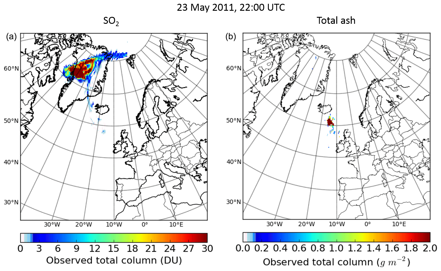
Figure 1 IASI SO₂ (a) and total ash (b) observations on 23 May 2011, 22:00 UTC.

For this study, three source terms, based on different assumptions and observational data, are applied in the model simulations. The emission scenarios range from (i) a simple approach, which assumes constant emission fluxes and a predefined vertical emission profile, to (ii) a more complex approach, which integrates temporarily varying observed plume heights and estimates emissions based on observed plume heights, to (iii) the most complex method that calculates temporal and vertical variability of the emission fluxes based on satellite observations and inversion techniques.

The remainder of this paper is divided into the following sections: Sect. 2 provides a technical description of the extension of the WRF-Chem volcanic emission preprocessor. Section 3 describes the WRF-Chem model setup and emission scenarios. The results and model evaluation with different observations (satellite, lidar, and surface air quality measurements) can be found in Sect. 4. Summary and conclusions are given in Sect. 5.

2 Extension of the volcanic preprocessor of the WRF-Chem model

The WRF-Chem model simulates emission, transport, mixing, and chemical transformation of trace gases and aerosols simultaneously with the meteorology. The model enables the use of various options for dynamic cores and physical parameterizations (Skamarock et al., 2008). The online approach (meteorology with air chemistry; see e.g. Baklanov et al., 2014) accounts for a numerically consistent air quality forecast.

In the official release of WRF-Chem v4.2 (code is available at https://github.com/wrf-model/WRF/releases, last access: 20 November 2020), volcanic emission sources can be considered only in a very simplified way. The model can simulate the dispersion of volcanic emissions specified by the initial plume height, erupted mass (ash and SO₂), duration of the eruption, and aerosol bin size distribution (up to 10 bin sizes).

If erupted mass is not known, it can be calculated applying the Mastin formula (Mastin et al., 2009), which relates plume height h_plume (in metres) to the emitted mass per time step m_emitted (kg/s).

$$\begin{array}{}\text{(1)}& m_{\mathrm{emitted}}=\mathrm{2600}\cdot (\mathrm{0.0005}\cdot h_{\mathrm{plume}}{)}^{\mathrm{4.1494}}\end{array}$$

For the vertical source term structure, a 75∕25 umbrella-shaped plume is applied: 25 % of the mass from vent height to a certain height (∼73 % of plume height) of the plume and then 75 % of the mass distributed to a parabolic distribution until plume-top height. For real-time applications, this is a straightforward approach, as the development of the volcanic emission cannot be predicted.

Stuefer et al. (2013) had extended the volcanic emission preprocessor with time-variant emissions, which can either be specified directly as mass fluxes or calculated with the Mastin equation based on temporarily varying plume heights (implemented in WRF-Chem version 3.4).

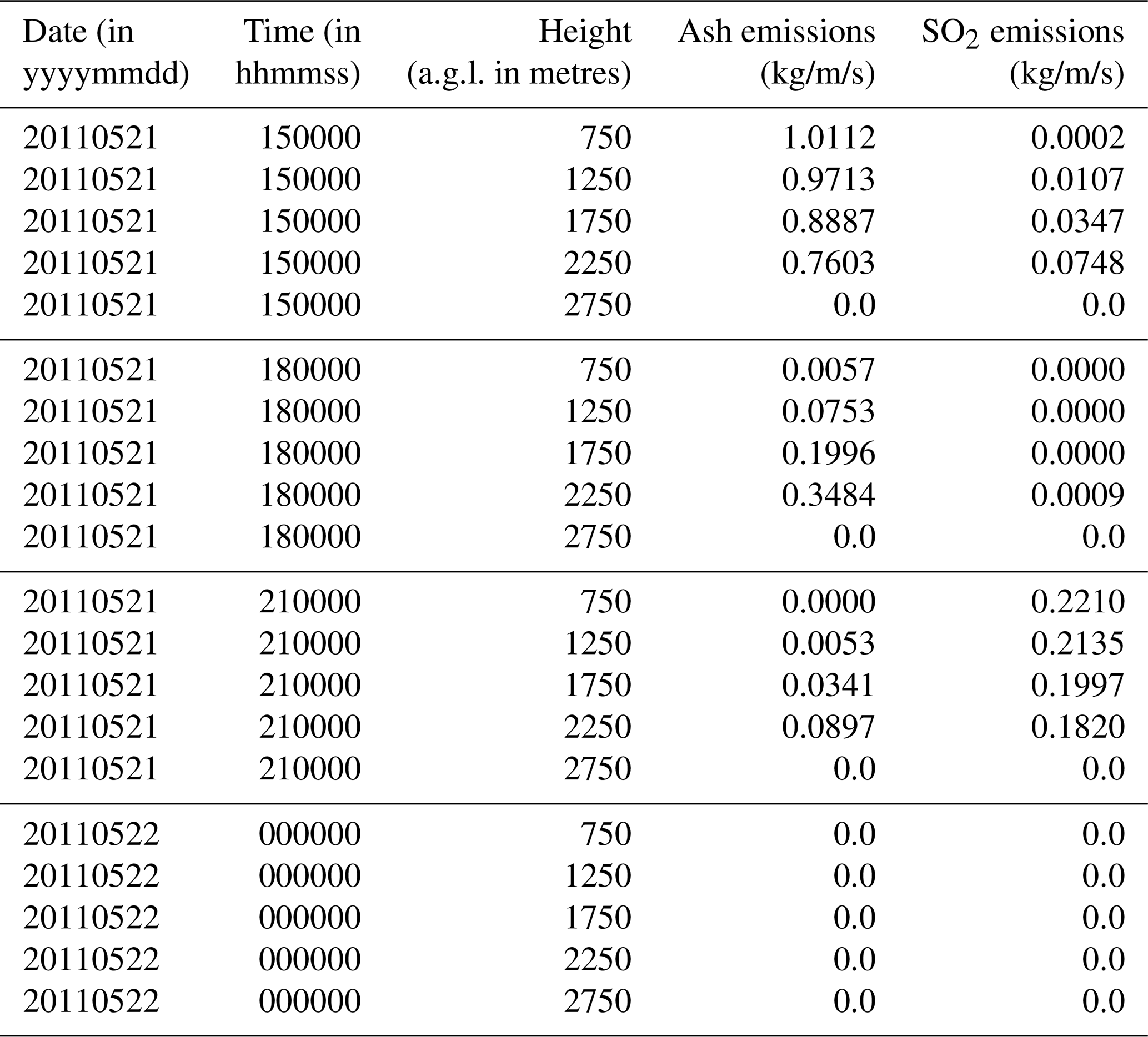
We extended the WRF-Chem capability towards user-defined volcanic source emission data that are read in through an external file. These emission fluxes (kg/m/s) comprise vertically resolved time series of ash and SO₂, as shown in Table 1. The date and time entries refer to the start of the emission interval, and the specified height (above ground level, AGL) refers to the lower limit of the height interval. Emissions of the last time step and the topmost level are the upper bounds of the highest sub-column and the last time step (therefore emissions are set to zero). The emission fluxes can be estimated by any suitable method. They can for example be produced with Bayesian inversion techniques, as included in the third emission scenario in this study.

Table 1 Example input data from the May 2011 Grimsvötn event for the new volcanic emission preprocessor.

As the emission fluxes have to be provided at heights above ground, the preprocessor (linearly) interpolates the input values for each column to the model levels of WRF-Chem (see Fig. 2). Depending on the difference between the model terrain height of the vent and the real vent height, an offset can be defined to account for deviations due to the limited model resolution. Finally, the resulting total volcanic emission, which is used for the WRF-Chem simulation is scaled in order to ensure mass conservation (can be violated due to interpolation effects). The routines have already been used in the frame of a volcanic eruption exercise for an artificial eruption of Etna (Hirtl et al., 2020).

Figure 2 Linear interpolation between input data (blue) and WRF-Chem model levels (green) of the emission flux (red, kg/m/s).

3 WRF-Chem model simulations

3.1 Model setup

WRF-Chem simulations were performed from 21 to 26 May 2011. The model domain extended from northern Africa to the north of Greenland and from eastern Newfoundland to western Russia. Model resolution was 12 km horizontally and 47 levels vertically from the surface up to 50 hPa. Meteorological fields used as initial and boundary conditions were derived from the European Centre for Medium-range Weather Forecasts (ECMWF). Parameterization of physical processes included the Mellor–Yamada–Nakanishi and Niino Level 2.5 planetary boundary layer (PBL) schemes (Hong et al., 2006), the Grell three-dimensional (3D) ensemble cumulus parameterization (Grell and Freitas, 2014), and the Rapid Radiative Transfer Model for Global (RRTMG) long-wave and short-wave radiation schemes (Iacono et al., 2008).

All simulations considered 10 volcanic ash bins and SO₂ (chem_opt =402). Total fine ash was assumed to be composed of the finest four bins (the other bins were set to zero): 12.7 % of particles within 0.01 to 3.9 µm in diameter, 18.2 % within 3.9 to 7.8 µm, 29.1 % within 7.8 to 15.6 µm, and 40.0 % within 15.6 to 31.0 µm. This is consistent with the FLEXPART (FLEXible PARTicle dispersion model; Stohl et al., 2005) model simulations that are used as input for the Bayesian inversion (emission scenario 3) to calculate an a posteriori source term (see Sect. 3.2). It uses the size distribution which represents the bin size range to which the IASI satellite observations are mainly sensitive to.

3.2 Volcanic emission scenarios

Three emission scenarios (further designated as S1, S2, and S3) were selected to test the sensitivity of ash and SO₂ dispersion to volcanic emissions. Underlying complexity of the source terms ranges from a very simple first guess to a sophisticated a posteriori source term, which was derived with satellite observations and inverse modelling.

Simple volcanic emission source terms can be derived from the eruption plume height (Mastin et al., 2009; see also Sect. 2). During the Grimsvötn eruption in 2011, plume height measurements were performed with weather radars (e.g. Petersen et al., 2012) and made available by the Icelandic Meteorological Office (IMO). The time series of observed plume heights AGL from the Keflavík radar is shown in Fig. 3.

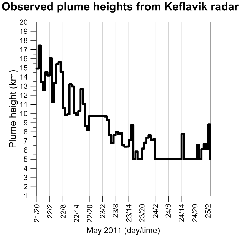
Figure 3 Observed plume heights (a.g.l.) from the Keflavík radar from 21 until 25 May 2011 during the eruption of the Grimsvötn volcano.

The first emission scenario (S1) used only the first observed plume height (15 km) and assumed constant emissions of ash and SO₂ for the eruption which was assumed to last 2 d. This is a very rough estimate, though a common approach to get a first idea of the dispersion of the volcanic plume. The associated uncertainties increase rapidly, in particular if eruption characteristics change. An ash emission rate of about 0.01 Tg/s was estimated with the Mastin formula (Eq. 1) for ash. For SO₂, the total emitted mass was assumed to be 1 Tg, yielding a constant emission rate of about 5787 kg/s for the 2 d. The vertical source term structure was modelled as a 75∕25 umbrella-shaped plume.

The second emission scenario (S2) was based on the entire observed plume height time series. The same plume heights were assumed for ash and SO₂ even though Prata et al. (2017) found that observed plume heights were more linked to SO₂ than to ash. Ash emission rates were computed with the Mastin equation for each time step. Based on the total amount of IASI ash and SO₂ measurements for the 4 d of the eruption, the hourly emission rates were further constrained with these satellite observations following Moxnes et al. (2014). The total emitted mass used in the simulations was scaled to 0.4 Tg for ash and to 0.36 Tg for SO₂. The magnitude of the SO₂ emission is reasonable, as shown by Flemming and Inness (2013), who estimated a total emitted mass of SO₂ of 0.32 Tg. After scaling, volcanic emission rates ranged from 67 to 12 080 kg/s for ash and from 60 to 10 872 kg/s for SO₂. The vertical structure of the source term was again modelled as a 75∕25 umbrella-shaped plume but considering different plume heights.

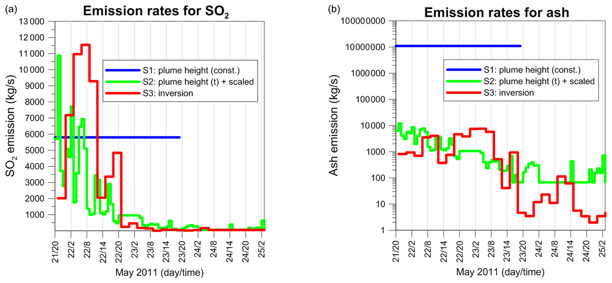
The third emission scenario (S3) uses the source terms produced with the Bayesian inversion technique, using FLEXPART runs and observations from the IASI instrument. The source term files were provided by Moxnes et al. (2014), who also described the method in detail. The source terms are shown in Fig. 4, with a vertical resolution of 1000 m. In contrast to S1 and S2, the vertical structure of these emissions does not follow an umbrella-shaped plume. While maximum SO₂ emissions (up to 11541 kg/s) were found at altitudes between about 5 and 12 km above sea level (a.s.l.) in the morning of 22 May, ash emissions were largest (7539 kg/s) at lower altitudes (below approximately 2 km a.s.l.) in the morning on 23 May.

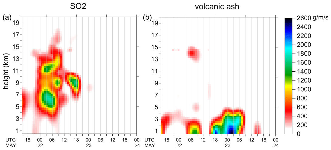
Figure 4 Temporal evolution of hourly-resolved vertical (height a.s.l.) SO₂ (a) and ash (b) emissions from FLEXPART inverse modelling based on IASI data. Data obtained from Moxnes et al. (2014).

According to Fig. 4, the highest ash emissions are below 5 km a.s.l., while the SO₂ emission peaks are located at altitudes between 5 and 13 km. Figure 5 summarizes the temporal evolution of the emission rates of all three scenarios. While SO₂ emissions are highest during the early phase of the eruption, the highest ash emissions occur after 22 May, 20:00 UTC, when SO₂ emissions are already low. The comparison of the three scenarios reveals average SO₂ emissions for the simple S1 source term but distinctively higher S1 ash emissions compared to S2 and S3 (note the logarithmic y axis).

Figure 5 Emission rates for all three emission scenarios for SO₂ (a) and ash (b).

3.3 Model inter-comparison of predicted ash considering aviation regulation aspects

To evaluate the performance of the three emission scenarios in a first step, the model runs are intercompared for the first 2 d of the eruption. Focus is set on ash concentration levels, which are important for aviation aspects. All regions with volcanic ash mass concentration greater than or equal to 4 mg/m³ are considered high-contamination areas (ICAO, 2016). Passenger aircraft are advised not to fly through regions of volcanic ash concentrations that exceed 4 mg/m³. This threshold is therefore most important for aviation aspects.

Figure 6 shows the 4 mg/m³ contour lines of maximum sub-column (between WRF-Chem model levels) volcanic ash for all emission scenarios for 22 and 23 May, 00:00 and 12:00 UTC. Since emission rates of scenario S1 are much higher than those of S2 and S3 (see Fig. 5), ash-rich regions are distinctively larger for S1 than for the other scenarios. This is most visible on 23 May, 12:00 UTC, when the S1 cloud spreads from Greenland and Iceland towards the UK. Neither the S2 nor the S3 scenario shows any significant area with an ash concentration exceeding 4 mg/m³. This illustrates how crucial it is to carefully estimate the emission rates. Comparison between scenarios S2 and S3 reveals a higher ash concentration on 22 May for S2 but lower ash contamination on the day after. This can be explained with corresponding emission rates (Fig. 5). An evaluation of the source-term performance and investigation of corresponding ash and SO₂ dispersion from all WRF-Chem simulations can be found in the next section, where model runs will be compared with independent observations.

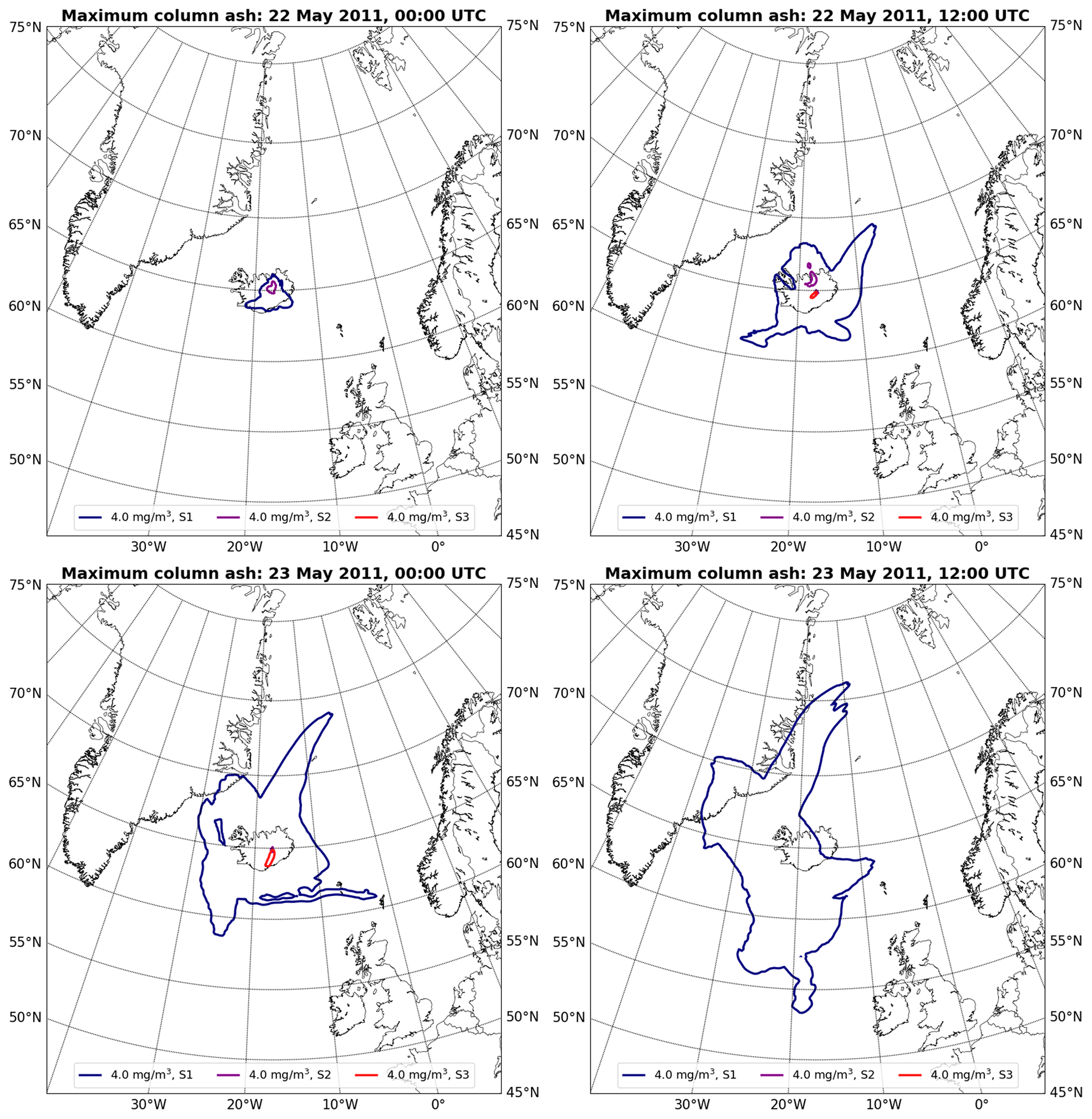
Figure 6 Maximum sub-column concentrations of total ash indicated via the 4 mg/m³ isoline for each grid cell predicted for the first 2 d (22 and 23 May 2011, 00:00 and 12:00 UTC) after the eruption start for the three emission scenarios simulated with WRF-Chem.

4 Evaluation of WRF-Chem simulations with observations

4.1 Comparison of volcanic ash and SO₂ with satellite data

In this section, the model simulations are compared to satellite observations of ash and SO₂ from different instruments. SEVIRI is an instrument on board the geostationary METEOSAT (Schmetz et al., 2002) satellite, which observes any point within its field of view every 15 min (over Europe every 5 min), AATSR was an instrument on board ENVISAT (mission ended in 2012), which was in a sun-synchronous orbit with an Equator crossing time of 10:00 local time. Several studies exist in which data of the two instruments have been used to analyse volcanic eruptions. Virtanen et al. (2014) have developed a (plume and cloud) height estimate algorithm for AATSR, which has been validated and compared to other satellite-based instruments and in situ data. The method was applied to the Eyjafjallajökull eruption in 2010 and performed reasonably well. Kylling et al. (2015) compared SEVIRI with IASI observations for the Grimsvötn eruption and found deviations in mass loadings of about a factor of 2 between the instruments, with the higher concentrations measured by SEVIRI, for the plume going northward.

Results from scenario S1 are not considered here because the model intercomparison already indicated a strong overestimation of ash simulated with S1 (Fig. 6). The model simulations for the scenarios S2 and S3 are compared to total column ash from SEVIRI and AATSR observations for 23 May 2011 in Fig. 7. The ash cloud was observed south of Iceland by both SEVIRI and aerosol optical thickness (AOT) from the AATSR, which were in good agreement. The simulation based on S3 performs well and reproduces the location of the cloud. The maximum total ash concentration based on S3 was higher than that of SEVIRI with 10.7 g/m² compared to 3.9 g/m², respectively. Based on S2, however, the highest ash concentrations (maximum 4.5 g/m²) are simulated in the northwest of Iceland due to wrong assumptions of the emitted ash-plume-top heights. On the next day (24 May; see Fig. A1) the scenarios S2 and S3 further drift apart, again with S3 being in better agreement with the observations. While most of the observed cloud moves towards the east (to the UK and Scandinavia), SEVIRI also detected some ash north of Iceland, which is assumed to be noise in the data, not present in AATSR and in the model. Ash mass loading of the cloud northeast of Scotland is as high as 3.7 g/m² in SEVIRI data and 0.8 g/m² in the S3 model run.

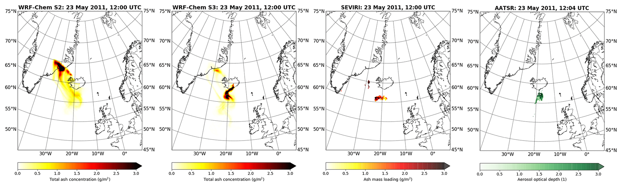
Figure 7 Total ash columns from WRF-Chem simulations (S2 and S3), SEVIRI ash mass loading and AOT from AATSR on 23 May 2011 12:00.

Observations from the AIRS instrument, a hyperspectral imager on the polar-orbiting EOS Aqua satellite, are used for comparison of SO₂. AIRS has a spatial resolution of 13.5 km and has already been used to study other volcanic eruptions, such as the Etna eruption in 2002, published by Carn et al. (2005). They showed that comparisons with MODIS observations indicated that AIRS is likely to underestimate SO₂ in the vicinity of the volcano due to the presence of dense ash.

Simulated SO₂ concentrations from all WRF-Chem runs and SO₂ observed by AIRS are shown in Fig. 8 for 23 May 2011. A total of 2 d after the eruption the SO₂ cloud was transported towards the north. All model scenarios reproduce this pattern in general but show differences in plume width and in the distance of the plume from the vent. AIRS data also showed SO₂, which was transported towards the east, but this could not be reproduced by the model simulations. The maximum observed SO₂ concentration was about 95 DU, which was detected northwest of Iceland. The highest SO₂ concentrations from model simulations range from about 60 DU in S2 to 910 DU in S1. During the next days (Fig. A2) differences between the model and the observations increase.

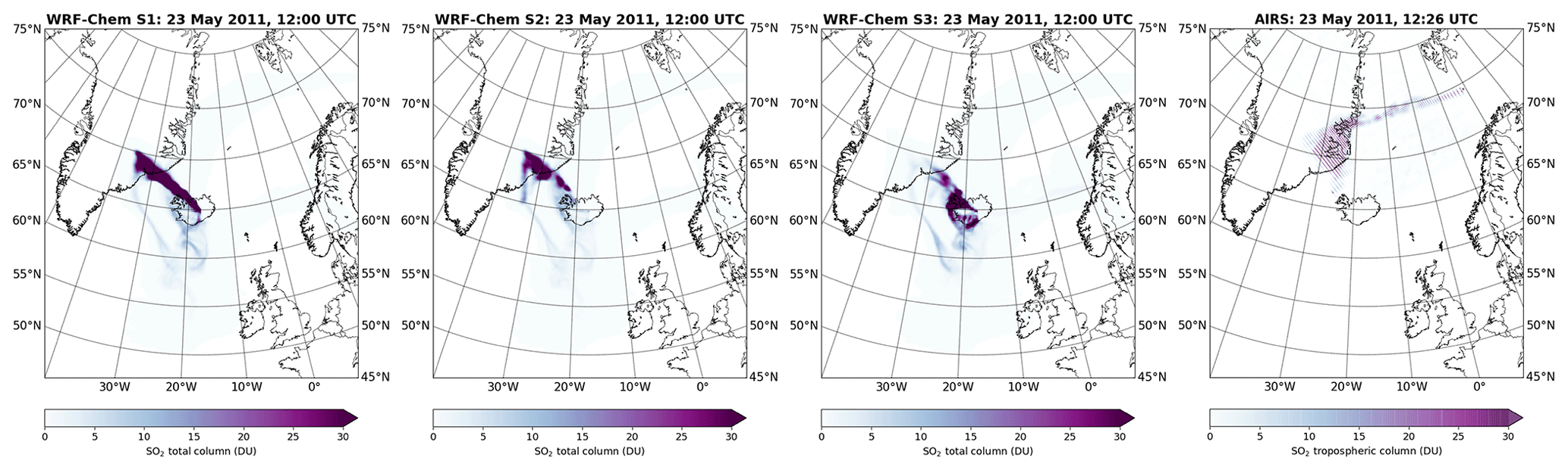
Figure 8 SO₂ total columns (DU) from WRF-Chem simulations (S1, S2, and S3) compared to the AIRS observations on 23 May 12:00.

The comparison of the WRF-Chem simulations with satellite observations revealed that the proper prediction of the location of the ash and SO₂ plumes for the Grimsvötn 2011 eruption is only possible when the source terms are treated separately.

4.2 Comparison with ground-based observations

Measurements from two lidar stations and several ground-based in situ observations are used to further evaluate the S3 model simulation. Both S1- and S2-based simulations did not show relevant ash concentrations at these locations.

4.2.1 Lidar profiles at selected stations

Vertical profiles of volcanic ash are compared with measurements from lidars (pink dots in Fig. 9) in Stockholm (Tesche et al., 2007; Althausen et al., 2009; Tesche et al., 2012) and Cabauw. On 24 May, the model simulates that a narrow, elongated band of ash was transported over the northern European mainland. The cloud ranged from the Netherlands up to northern Scandinavia (Fig. 9). It slowly approached Stockholm (Fig. 9 northern pink dot), where maximum ash column concentrations were found at about 23:00 UTC.

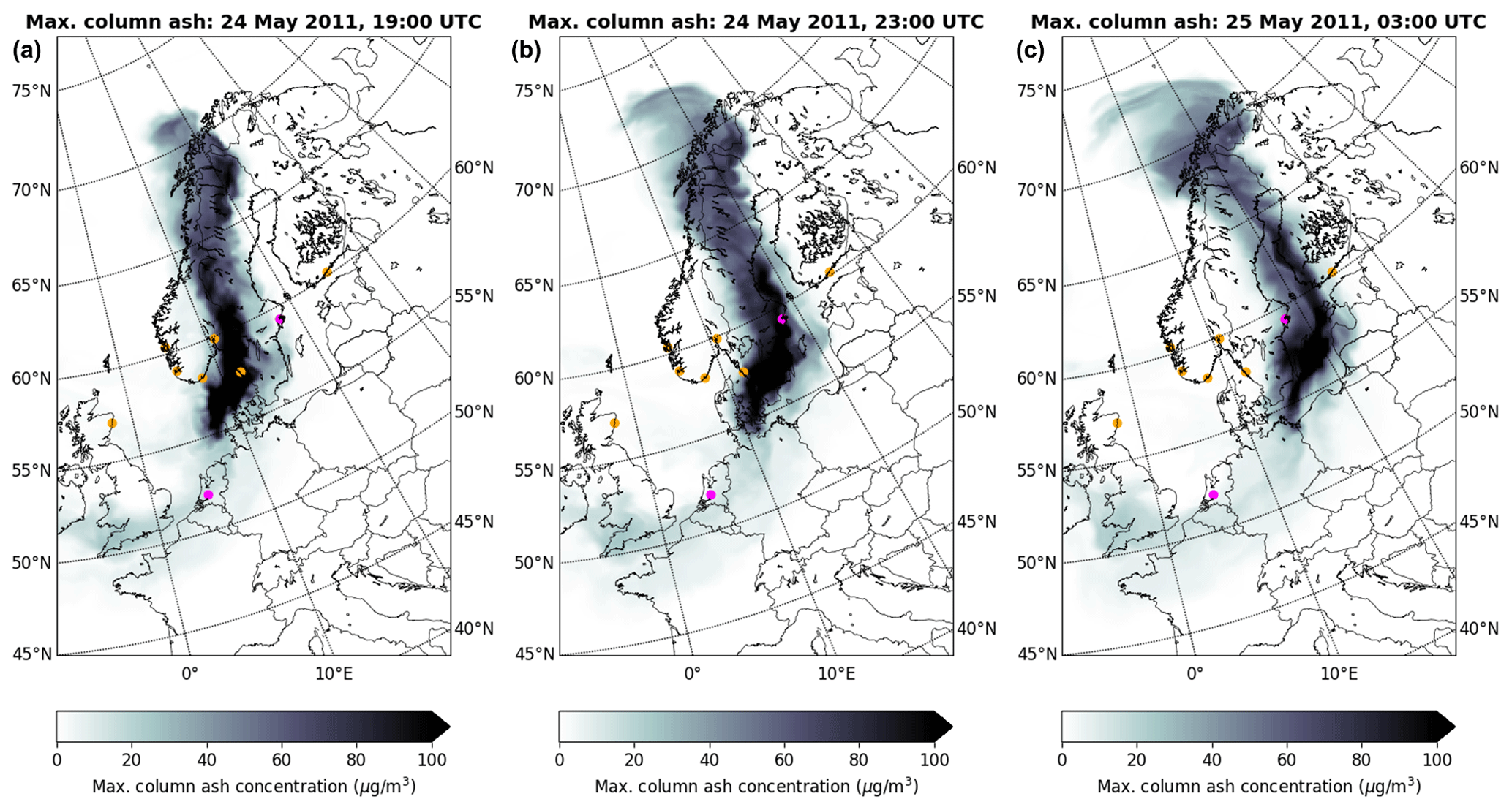
Figure 9 Simulated maximum total ash column for each grid cell on 24 May at 19:00 (a), 23:00 (b), and 25 May 03:00 UTC (c). The pink dots indicate the locations of the lidar in Stockholm and Cabauw, and the orange dots indicate the location of the ground stations.

The lidar measurements in Stockholm (Fig. 10) revealed ash arrival a few hours later, on 25 May between 03:00 and 04:00 UTC. The temporal offset is, however, relatively small, considering that Stockholm is far away from the source region and that the ash cloud has already been transported for a couple of days.

Figure 10 Min–max observed ash concentrations values at the lidar Stockholm (25 May 02:00 until 08:00) compared to the WRF-Chem maximum ash concentrations (24 May 19:00 until 25 May 03:00 UTC) for each vertical level.

The vertical profile of modelled maximum ash concentration (average from 24 May 19:00 UTC until 25 May 03:00 UTC) based on S3 over Stockholm is below the ash mass concentration estimates from Tesche et al. (2012) that were based on lidar measurements between 02:00 and 08:00 UTC. While the model predicts maximum ash concentrations (<100 µg/m³) within a thick vertical layer between 500 and 2500 m, the lidar observations revealed a sharp peak at about 1000 m with values between 50 µg/m³ (lower estimate) and 450 µg/m³ (upper estimate). The maximum (as well as the minimum) curve is based on different assumptions when calculating the mass from the extinction coefficient. According to Tesche et al. (2012), the minimum curve is more likely to represent the real observed ash concentrations.

Volcanic ash was also detected by the lidar at Cabauw on 25 May, 16:30 UTC. Figure 11 shows a qualitative comparison of the observed backscattering coefficient profile and the S3-based modelled ash concentration profile, both normalized to 1. Both data sets clearly show enhanced aerosol concentrations between about 500 and 2000 m with the peaks at 1250 and 1500 m in the lidar and model data, respectively. The predicted vertical extension of the ash layer shows a very good agreement with the observation at the Cabauw station.

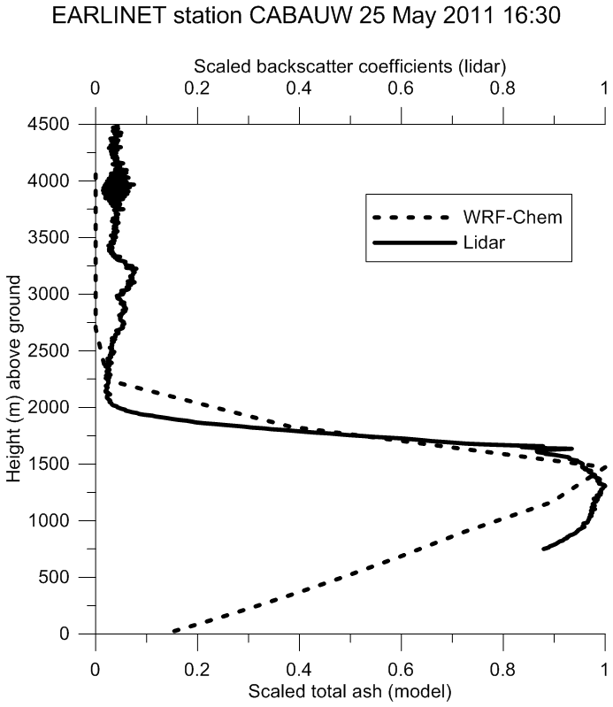
Figure 11 Vertical (scaled) profiles of WRF-Chem S3-based total ash and backscattering coefficients from the EARLINET lidar at Cabauw on 25 May 2011, 16:30 UTC.

4.2.2 Comparison with PM₁₀ observations at selected ground stations

For the days of the Grimsvötn eruption, surface measurements of PM₁₀ are available from several stations in northern Europe (orange dots in Fig. 9). These data have already been used by others to investigate the eruption and to evaluate dispersion models (e.g. Prata and Prata, 2012; Tesche et al., 2012; Moxnes et al., 2014). The WRF-Chem output (the finest three ash bins corresponding to the size range of PM₁₀) from scenario S3 was interpolated to the station locations and compared for the 2 d of the volcanic ash cloud overpass on 24 and 25 May. Figure 12 shows the time series of the observed hourly data for the stations.

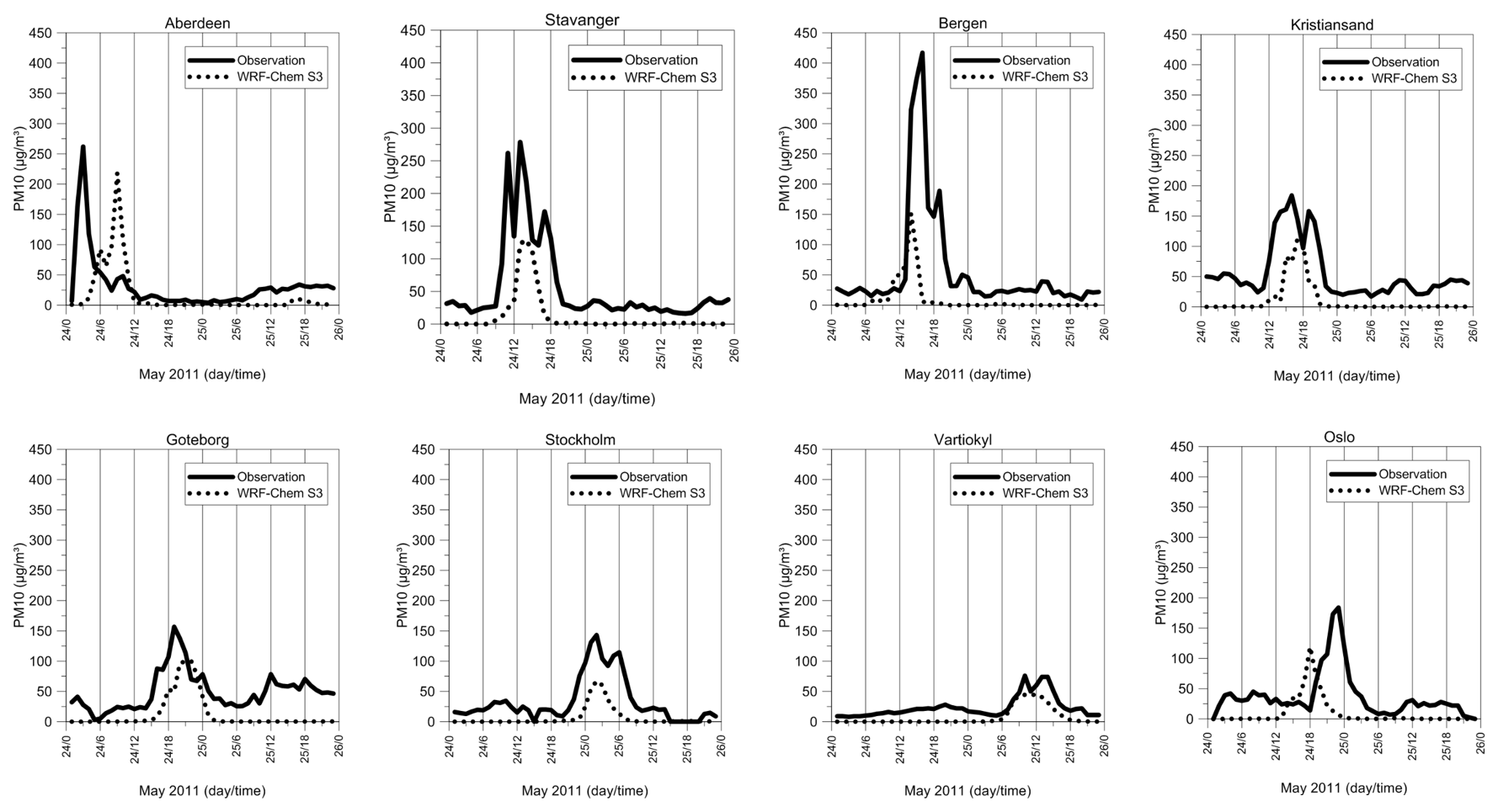
Figure 12 Time series of observed PM₁₀ (µg/m³) ground concentrations (solid line) and WRF-Chem (S3) simulations (dotted line) for 24 and 25 May 2011.

In general, the observed PM₁₀ concentrations are slightly higher than the model prediction. This is not only true for PM₁₀ peaks, when a large portion of PM₁₀ can be attributed to volcanic ash, but also for the entire time period. This model bias is caused by missing anthropogenic and biogenic aerosol emissions as well as secondary aerosol formation yielding zero PM concentrations before and after the volcanic ash overpass. These contributions were not considered in the simulations as the emphasis of this study was on the ash and SO₂ emitted by the volcano.

For most of the ground stations, the plume arrival is simulated well by the model, although the model underestimates the observations. In Aberdeen, a temporal shift of about 6 h is observed. At this station the modelled peak is later compared to the observed peak. This is in contrast to the station in Oslo where the simulated peak arrives about 6 h earlier. The ground observations in Stockholm reveal that the time of the plume arrival is captured by the model very well in contrast to the lidar observation, which indicates a temporal shift of about 4 h.

Note that the simulation of the dispersion of ash and SO₂ over long distances is subject to large uncertainties. Uncertainty in the emission and the meteorology (e.g. vertical mixing) has a strong impact on the dispersion and causes deviations between model and observations, especially for this complex case.

5 Conclusions

The developments presented in this paper permit the integration of complex source profiles into the emission preprocessor of the WRF-Chem model. Such temporarily and vertically resolved emissions of ash and SO₂ can be obtained, e.g. by inverse modelling exploiting satellite observations. The simple structure of the input data format allows integration of source term characteristics from any suitable method.

Model runs with three emission scenarios were conducted and evaluated for the eruption of the Grimsvötn volcano in 2011. This eruption was unique because ash and SO₂ injection heights were separated and a vertical wind shear led to different transport directions of the respective clouds after the eruption. Model performance for ash and SO₂ dispersion was therefore highly sensitive to the source geometry.

The first model scenario neglected different emission geometries of ash and SO₂. It used the first observed plume height (15 km) as plume-top height for ash and SO₂ and assumed constant emission fluxes for the entire eruption period which was estimated to last for 2 d. Emission fluxes were calculated empirically (Mastin et al., 2009) and distributed vertically in a 75∕25 umbrella-shaped plume (Stuefer et al., 2013). The second scenario was based on the entire observed plume-top-height time series, which was, again, assumed to be the same for ash and SO₂. After scaling empirically derived emission fluxes (Moxnes et al., 2014), emitted mass was distributed again in a 75∕25 umbrella-shaped plume while considering different plume heights. The third scenario was based on emission fluxes obtained by the inversion of volcanic ash and SO₂ column observations from the IASI instrument applying the FLEXPART model to link an a priori source term and satellite total column observations. This source term includes different emission characteristics of ash and SO₂, both in the temporal and in the vertical dimensions.

Evaluation of the model simulations revealed the best performance of the most complex third emission scenario (S3). Improper emission heights of scenario 1 (S1) resulted in overestimated emission fluxes and produced too high ash concentrations. Furthermore, the ash cloud dispersed into the wrong direction. For the second emission scenario (S2), the simulated magnitudes of the concentrations of ash and SO₂ were in good agreement with the satellite observations, although the location of the ash cloud was wrong due to incorrect ash plume-top heights, which were in reality lower than those of SO₂. This underpins the utility of separate ash and SO₂ source terms with reasonable temporal and vertical variability as used in S3. This simulation did not only reproduce the location of ash and SO₂ clouds correctly, but also ash concentration values close to the surface.

Validation of simulated vertical ash concentration profiles also revealed a good agreement with observations, although the ash cloud was dispersed already for a few days on the way to the measurement locations. The PM₁₀ fraction of the ash was compared to ground stations in northern Europe. The model underestimates the observations because no other PM₁₀ sources (anthropogenic, biogenic, sea salt, etc.) were considered in the simulations. The prediction of the cloud overpass time was well accomplished for most of the stations by the model run using the complex emission source term S3.

Our analysis showed that volcanic ash can also have an impact on air quality when the cloud touches the ground. Especially for volcanic events which significantly affect surface air pollution, forecast models can support authorities to warn the public.

Fast access to on-site measurements, e.g. from volcano observatories, is important to constrain dispersion models during an emergency crisis. Decisions must be based on the best available information. Updated source term estimates and model hindcasts can help to better understand and predict the transport of ash and gases. Volcanic ash observations from satellite instruments are sometimes limited in accuracy; thus models may help to interpret satellite retrievals. This is crucial for the aviation sector, which is highly vulnerable to “airborne” hazards. Accurate model predictions are not only important to ensure aircraft safety, but can also avoid air space closures or flight reroutings, which can save millions of dollars.

Appendix A

Figure A1 Total ash columns from WRF-Chem simulations (S2 and S3), SEVIRI ash mass loading, and AOT from AATSR on 22 to 24 May 2011 12:00.

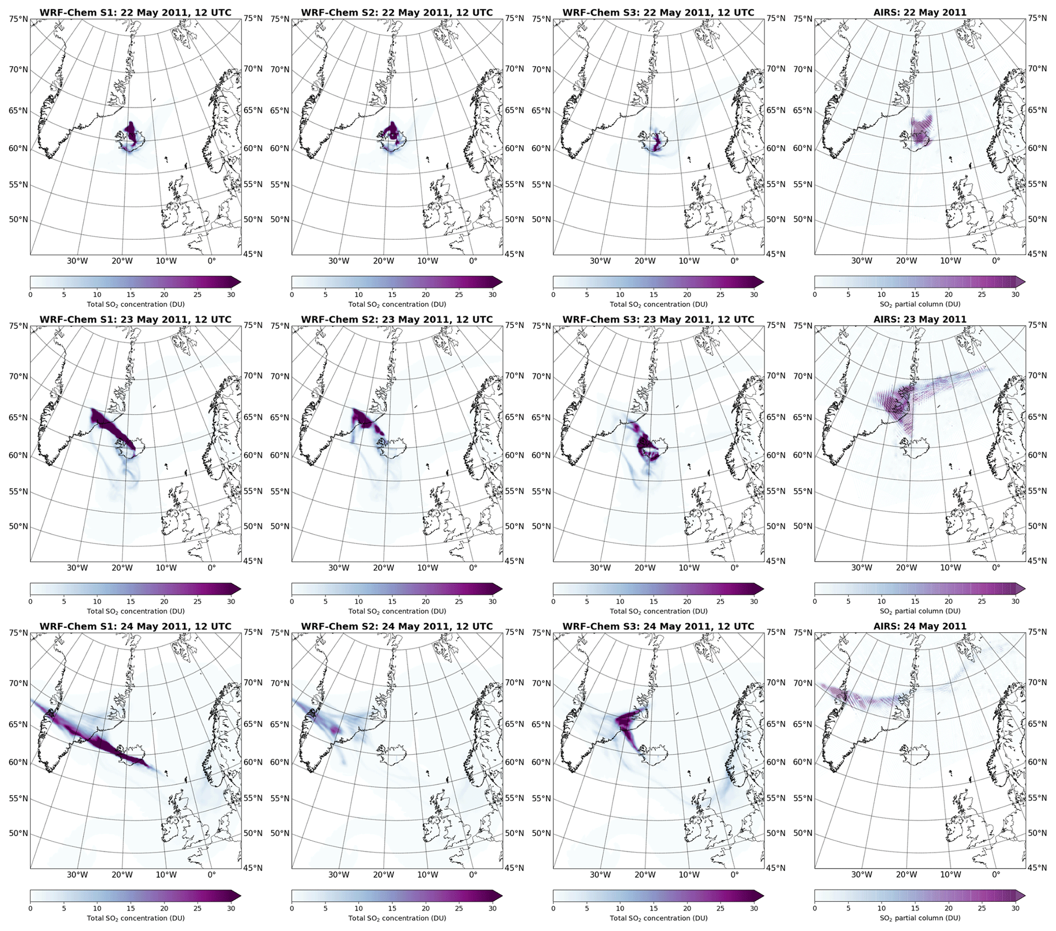
Figure A2 SO₂ total columns (DU) from WRF-Chem simulations (S1, S2, and S3) compared to the AIRS observations on 22 to 24 May 12:00.

Appendix B: Glossary

AATSR	Advanced Along-Track Scanning Radiometer
a.g.l.	Above ground level
a.s.l.	Above surface level
AIRS	Atmospheric Infrared Sounder
AOT	Aerosol optical thickness
DU	Dobson units
ECMWF	European Centre for Medium-Range Weather Forecasts
EARLINET	European Aerosol Research Lidar Network
ENVISAT	Environmental Satellite
EOS	Earth Observing System
EUNADICS-AV	European Natural Airborne Disaster Information and Coordination System for Aviation
FLEXPART	FLEXible PARTicle dispersion model
GOME-2	Global Ozone Monitoring Experiment
IASI	Infrared Atmospheric Sounding Interferometer
ICAO	International Civil Aviation Organization
IMO	Icelandic Meteorological Office
Lidar	Light detection and ranging
METEOSAT	Meteorological satellite
MODIS	Moderate Resolution Imaging Spectroradiometer
NOAA	National Oceanic and Atmospheric Administration
OMI	Ozone Monitoring Instrument
PBL	Planetary boundary layer
PM	Particulate matter
RRTMG	Rapid Radiative Transfer Model for Global radiation schemes
SEVIRI	Spinning Enhanced Visible Infra-Red Imager
UTC	Coordinated universal time
VAACs	Volcanic Ash Advisory Centres
VACP	Volcanic Ash Contingency Plan
VAST	Volcanic Ash Strategic initiative Team
WRF-Chem	Weather Research and Forecasting (WRF) model coupled with Chemistry