the Creative Commons Attribution 4.0 License.
the Creative Commons Attribution 4.0 License.
 | 06 Nov 2020
Measuring the seismic risk along the Nazca–South American subduction front: Shannon entropy and mutability
Eugenio E. Vogel
Felipe G. Brevis
Denisse Pastén
Víctor Muñoz
Rodrigo A. Miranda
Abraham C.-L. Chian
Four geographical zones are defined along the trench that is formed due to the subduction of the Nazca plate underneath the South American plate; they are denoted A, B, C and D from north to south; zones A, B and D had a major earthquake after 2010 (magnitude over 8.0), while zone C has not, thus offering a contrast for comparison. For each zone, a sequence of intervals between consecutive seisms with magnitudes greater than or equal to 3.0 is set up and then characterized by Shannon entropy and mutability. These methods show a correlation after a major earthquake in what is known as the aftershock regime but show independence otherwise. Exponential adjustments to these parameters reveal that mutability offers a wider range for the parameters to characterize the recovery compared to the values of the parameters defining the background activity for each zone before a large earthquake. It is found that the background activity is particularly high for zone A, still recovering for zone B, reaching values similar to those of zone A in the case of zone C (without recent major earthquake) and oscillating around moderate values for zone D. It is discussed how this can be an indication of more risk of an important future seism in the cases of zones A and C. The similarities and differences between Shannon entropy and mutability are discussed and explained.
- Article
(4982 KB) - Full-text XML
- BibTeX
- EndNote


A recent advance in information theory techniques, with the introduction of the concept of mutability (Vogel et al., 2017a), opens new ways of looking at the tectonic dynamics in subduction zones. The main goals of the present paper are five-fold: (1) to establish the similarities and differences between mutability and the well-known Shannon entropy to deal with seismic data distributions; (2) to find out which of the aforementioned parameters gives an advantageous description of the subduction dynamics in order to discern different behaviors along the subduction trench; (3) to apply this description to characterize the recovery regime after a major earthquake; (4) to use this approach to establish background activity levels prior to major earthquakes; and (5) to apply all of the above to different geographical zones to look for possible indications of regions with indicators pointing to possible future major earthquakes.
Several statistical and numeric techniques have been proposed to analyze seismic events. For a recent review, we refer the interested reader to the paper by de Arcangelis et al. (2016) and references therein. We shall concentrate here on the use of Shannon entropy and mutability, which are introduced and discussed in the next paragraphs; they will be applied to the intervals between consecutive seisms in each region.
Data may come from a variety of techniques used to record variations in some earth parameters like infrared spectrum recorded by satellites (Zhang and Meng, 2019), earth surface displacements measured by Global Positioning System (GPS) (Klein et al., 2018), variations of the earth's magnetic field (Cordaro et al., 2018; Venegas-Aravena et al., 2019) and changes in the seismic electric signals (Varotsos and Alexopoulos, 1984a; Varotsos and Lazaridou, 1991; Varotsos, 2005; Varotsos et al. 1986, 1993, 2001, 2011c, 2019; Sarlis et al., 2018c), among others. In the present work, we make use of the seismic sequence itself like in natural time analysis (see, e.g., Varotsos et al., 2001, 2002, 2011a, b) to analyze the time intervals between filtered consecutive seisms.
Shannon entropy is a useful quantifier for assessing the information content of a complex system (Shannon, 1948). It has been applied to study a variety of nonlinear dynamic phenomena such as magnetic systems, the Rayleigh–Bénard convection, the 3D magnetohydrodynamics (MHD) model of plasmas, and turbulence or seismic time series, among others (Crisanti et al., 1994; Xi and Gunton, 1995; Cakmur et al., 1997; Chian et al., 2010; Miranda et al., 2015; Manshour et al., 2009).
Analysis of the statistical mechanics of earthquakes can provide a physical rationale for the complex properties of seismic data frequently observed (Vallianatos et al., 2016). A number of studies have shown that the complexity in the content information of earthquakes can be elucidated by Shannon entropy. Telesca et al. (2004) applied Shannon entropy to study the 1983–2003 seismicity of central Italy by comparing the full and the aftershock-depleted catalogues and found clear anomalous behavior in stronger events, which is more evident in the full catalogue than in the aftershock-depleted one. De Santis et al. (2011) used Shannon entropy to interpret the physical meaning of parameter b of the Gutenberg–Richter law that provides a cumulative frequency–magnitude relation for the statistics of the earthquake occurrence. Telesca et al. (2012) studied the interevent time and interevent distance series of seismic events in Egypt from 2004 to 2010 by varying the depth and the magnitude thresholds.
Telesca et al. (2013) combined the measures of the Shannon entropy power and the Fisher information measure to distinguish tsunamigenic and non-tsunamigenic earthquakes in a sample of major earthquakes. Telesca et al. (2014) applied the Fisher–Shannon method to confirm the correlation between the properties of the geoelectrical signals and crust deformation at three sites in Taiwan. Nicolis and Mateu (2015) adopted a combined Shannon entropy and wavelet-based approach to measure the spatial heterogeneity and complexity of spatial point patterns for a catalogue of earthquake events in Chile. Bressan et al. (2017) used Shannon entropy and fractal dimensions to analyze seismic time series before and after eight moderate earthquakes in northern Italy and western Slovenia.
In the last 2 decades, the concept of “natural time” for the study of earthquakes has been introduced by Varotsos et al. (1984b), Varotsos and Lazaridou (1991), and Varotsos et al. (1993, 2011a, b, c). This method proposes a scaling of the time in a time series by using the index , where k indicates the occurrence of the kth event and N is the total number of the events in a time series. For example, for seismic time series, the evolution of the pair (χk,M0k) is followed, where M0k is proportional to the energy released in an earthquake, finding interesting results in the seismic electric signal prior to an earthquake's occurrence (Sarlis et al., 2013, 2015, 2018a, b; Rundle et al., 2018). An entropy has been defined in natural time (Varotsos et al., 2011b) – being dynamic and not static (Varotsos et al., 2003, 2007) – by , and it has been very useful in the analysis of global seismicity (Rundle et al., 2019).
On the other hand, the method based on information theory (Luenberg, 2006; Cover and Thomas 2006; Roederer, 2005) was introduced a decade ago when it was successfully used to detect phase transitions in magnetism (Vogel et al., 2009, 2012; Cortez et al., 2014). A new data compressor was then designed to recognize compatible data, namely, data based on specific properties of the system. This method required comparing strings of fixed length and starting always at the same position within the digits defining the stored record. For this reason, it was named “word length zipper” (wlzip for short) (Vogel et al., 2012). The successful application of wlzip to the 3D Edwards–Anderson model came immediately afterwards, in which one highlight was the confirmation of a reentrant transition that is elusive for some of the other methods (Cortez et al., 2014). Another successful application of critical phenomena was for the disorder to nematic transition that occurs for the depositions of rods of length k (in lattice units) on square lattices: for k≥7, one specific direction for depositions dominates when the deposition concentration overcomes a critical minimum value (Vogel et al., 2017b).
Furthermore, wlzip proved to be useful not only for the case of phase transitions. It has been used in less drastic data evolution revealing different regimes or behaviors of a variety of systems. The first of such applications was in econophysics dealing with stock markets (Vogel and Saravia, 2014) and pension systems (Vogel et al., 2015). The alteration of blood pressure parameters was also investigated using wlzip (Contreras et al., 2016). At a completely different timescale, the time series involved in wind energy production in Germany was investigated by wlzip, which yielded recognition of favorable periods for wind energy (Vogel et al., 2018).
The first application of wlzip to seismology came recently using data from a Chilean catalogue that found that wlzip results clearly increase several months prior to large earthquakes (Vogel et al., 2017a), thus being in accordance with natural time analysis which reveals (Varotsos et al., 2011b) that before major earthquakes, there is a crucial timescale of around a few to several months in which changes in the correlation properties of physical quantities like seismicity or crustal deformation are observed. This early application of wlzip intended to establish the method without attempting further analyses or comparison with other methods or comparing possible seismic risk among regions, which are among the aims of the present paper.
In the present paper, we make a new analysis comparing results from mutability and Shannon entropy applied to seismic data along the subduction front parallel to the Chilean coast. The complete tectonic context shows an active and complex seismic region for all the coast driven by the convergence of the Nazca plate and the South American plate at a rate of 68 mm yr−1 (Altamimi et al., 2007) approximately. In the last 100 years, many large earthquakes have been localized in the shock between these two plates, such as Valparaíso 1906 (Mw=8.2), Valdivia 1960 (Mw=9.6), Cobquecura 2010 (Mw=8.8), Iquique 2014 (Mw=8.2) and Illapel 2015 (Mw=8.4). So this zone is an attractive source for studying seismic activity associated with large earthquakes. Although the dynamics along the Chilean coast may be dominated by the interaction between these two plates, various works have pointed out variations along the coast which may yield information about the details of that interaction. For instance, the coupling between these two plates has been studied by Métois et al. (2012, 2013) in recent years, concluding that the subduction area has alternating zones of high and low coupling (Métois et al., 2012, 2013). This suggests that it is interesting to apply novel nonlinear techniques to study such variability. Here, we propose new ways to characterize some of the various dynamics that may be present along the subduction zone in this trench. In order to do that, we will consider four regions along the coast of Chile characterizing them mainly by their latitudes.
The paper is organized in the following way. The next section is about the methodology dealing with the data and parameters to be measured. Section 3 presents the results, discusses them and compares the alternative methods. Section 4 is devoted to conclusions.
2.1 Data organization
Earthquakes originating in the subduction zone of the Nazca plate underneath the South American plate have been recorded, interpreted and stored in several seismic data banks. In the present study, we shall use the data collected by the Chilean National Seismic Center (CNS; Centro Sismológico Nacional) (web site of Servicio Sismológico Nacional, 2019), which are very accurate regarding the location of the epicenters. In particular, we have used a seismic dataset collected from March 2005 until March 2017, containing 22 697 events distributed along the coast of Chile from Arica in the far north down to Temuco in the south of Chile. These data are freely available through CNS (http://www.sismologia.cl).
In order to analyze the spatial evolution of the mutability and Shannon entropy along this part of the subduction zone, we have focused our attention on four regions defined below. For each region, we have corroborated that the Gutenberg–Richter law holds, finding a common completeness magnitude of Mw=3.0. Thus, all the following analysis will be made using only the seismic events with magnitudes of at least Mw=3.0. We have considered seismic data sequences for four specific geographical zones: three of them include one earthquake over 8.0 occurring after 2010, and we have added for comparison a neighboring area with no such large earthquake for several recent years.
Starting from the north, the zones are the following: (A) around the earthquake near Iquique (2014; Mw=8.2) comprising 6891 events, (B) around the earthquake near Illapel (2015; Mw=8.4) comprising 6626 events, (C) a quieter geographical region (calm zone) in the center of Chile (where the greatest seismic event is Mw=6.5) comprising 2824 events, and (D) around the earthquake in Cobquecura (2010; Mw=8.8) comprising 6356 events. The observation time is from 1 January 2011 to 23 March 2017 for zones A, B and C, while it is from 1 January 2009 to 23 March 2017 for zone D (no special reason for this last date). We extended the analysis in the case of zone D to include the regime prior to the big earthquake of 2010. Since the analysis is either relative to the size of the sample or dynamic along the series, this difference should not affect the discussion below.
All zones have a similar geographical extension with some singularities that we explain here. Regions A, B and D have latitudes centered at the epicenter of the largest earthquake of each zone; the span in longitude is the same for these zones. Zone A misses the 4.0∘ spans in latitude of zones B and D since the Chilean catalogue ends at , which is the northern limit for this zone (for homogeneity of the data, we do not mix catalogues). The largest span for the zones under study is 4∘ in each direction; it was chosen as a mean to consider enough data within each zone in order to have good statistics. On the other hand, zone C was chosen to include a populated area of the country but with no earthquake over 8.0 and to show less important activity than previous ones. Details are given in Table 1 and are illustrated in Fig. 1. As can be seen in this map, zone C overlaps with both B and D; to avoid getting close to the epicenter of the main earthquake in zone D, zone C was shortened in its southward extension. So the data catalogues have been filtered by latitude, longitude and magnitude. At this point, we do not filter by depth which should not greatly influence the comparison among zones since it is a common criteria for all of them.
Table 1Geographical definition of the four zones considered in this study. The strongest seismic event in each zone is identified at the end. Zone C lacks a very strong seism during recent years which is indicated by the use of parenthesis for the strongest seism here. The geographical coordinates and time windows are explained and defined in the text.

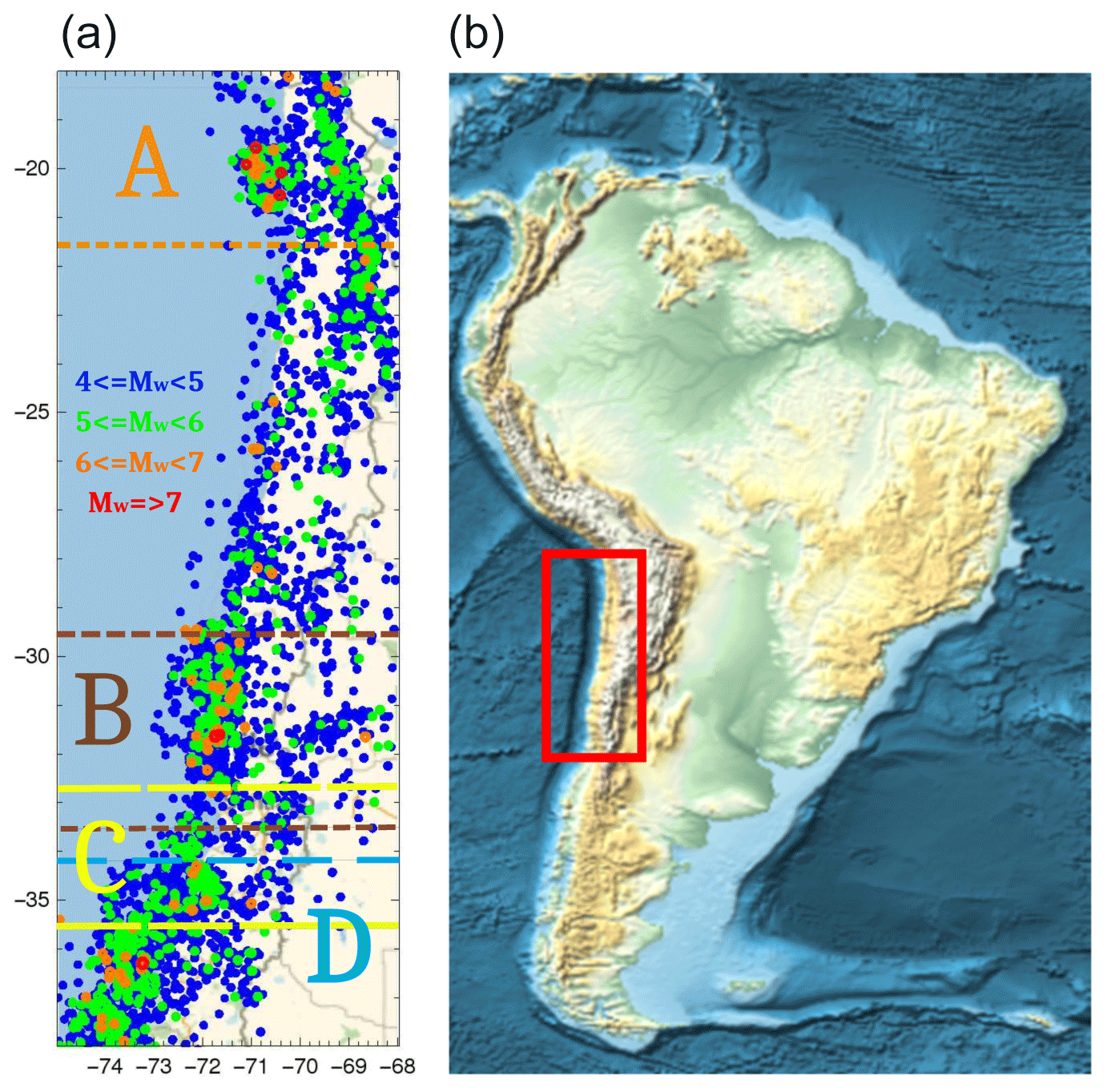
Figure 1(a) Map showing the seismic events with magnitudes greater than Mw 4.0 and the division in four geographical zones A, B, C and D defined in Table 1. The seismic events are shown by circles using the following color code according to magnitude: between 4.0 and 4.9 in blue, between 5.0 and 5.9 in green, between 6.0 and 6.9 in orange, and for a magnitude equal to or greater than Mw 7.0 in red. (b) Map of South America showing with a red rectangle the area displayed in the figure to the left. The trench between the South American plate and the Nazca plate appears in dark blue.
Originally, the study considered zones A, B and D only by concentrating on the main three earthquakes of the decade. Despite the main purposes of this work being accomplished by looking at zones A, B and D only, we decided to broaden the geographical coverage a bit. The area in between zones B and D could be unstable as subductions took place both south and north of it. Eventually, the subduction here is stuck, and it could be interesting to find out the behavior of this densely populated zone. We paid the price of overlapping with the neighboring zones, but special care has been taken to avoid in zone C the epicenters and immediate vicinity of the major earthquakes and to initiate the analysis in 2011, several months after the largest earthquake included in this study.
For all seismic events characterized above, we calculate the interval in minutes (rounding off seconds) between consecutive events. Then a vector file is produced storing the consecutive intervals between theses seisms within each zone. These are the files to be analyzed by Shannon entropy and mutability. Notice that there is a close similarity between this and the “natural time” analysis discussed in the Introduction since the resulting vector is indexed by the event number. In our case, the value of each vector component is the interevent time itself, which has also been used in the natural time analysis of electrocardiograms by considering the interevent time between consecutive heartbeats (Varotsos et al., 2007). Registers in the vector storing the information in our analysis are the interevent intervals; thus, temporal information is still kept in the time series.
Let us consider histograms for interval distributions for each zone with consecutive bins of 60 min each. The percentage of abundance GK,i of intervals are obtained for the ith bin for the different zones Z: A, B, C or D. Figure 2 shows the histograms corresponding to the distribution functions GZ,i. It can be immediately seen that shorter intervals have been more frequent in zones D and B, while they are less frequent in zone C. Zone A presents an intermediate presence of small intervals. This different frequency for small seisms is explained by in the presence of large earthquakes in B and D followed by large aftershock periods, while in zone A the aftershock period (and the number of short intervals) was very short, as we will see in detail below. Zone C does not include any aftershock period, so short intervals are less frequent here.
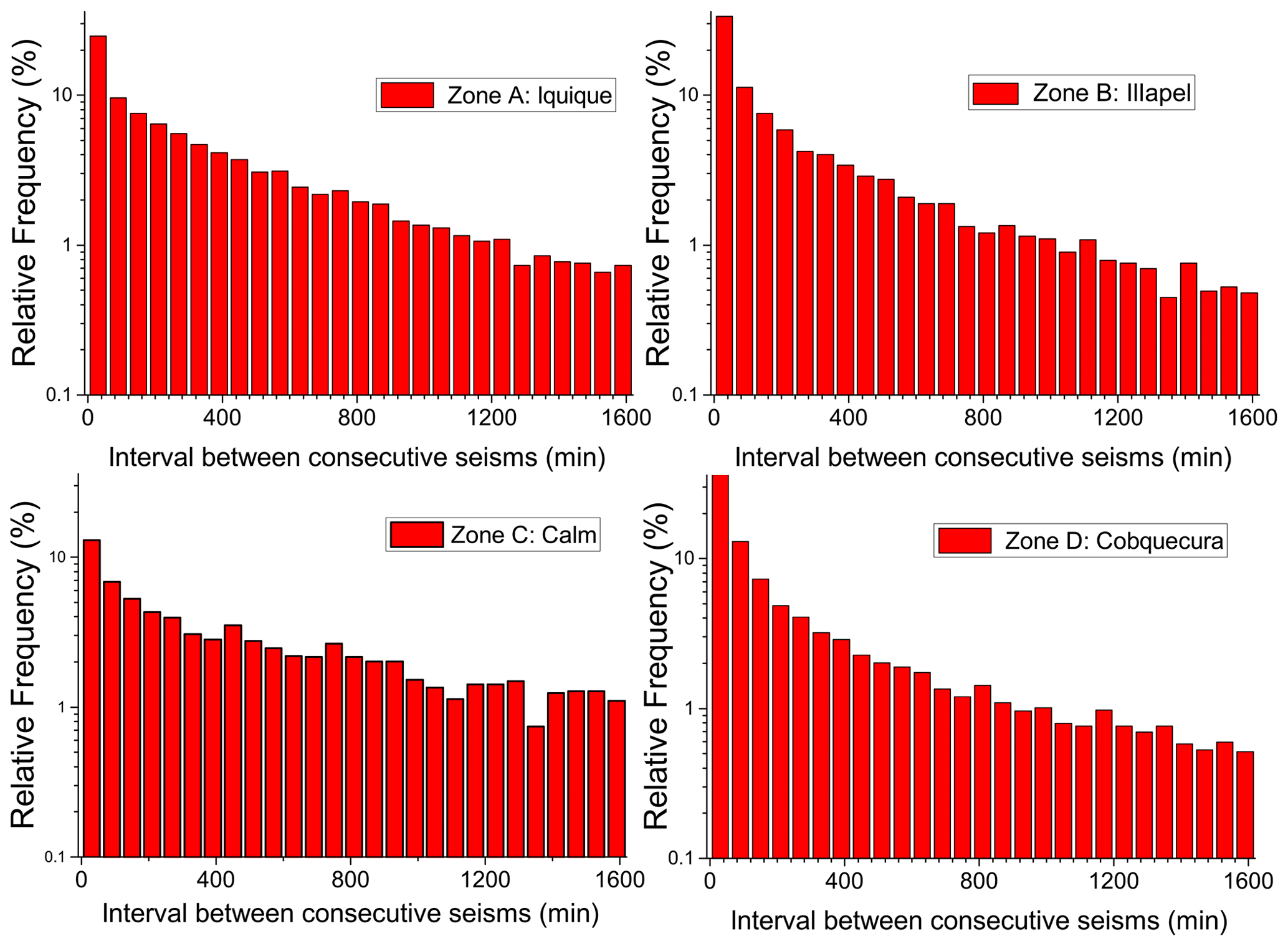
Figure 2Distribution functions GZ,i (Z = {A, B, C, D}) for intervals between two consecutive seismic events.
To better establish the role of the aftershocks, we compared the number of seisms (3.0+) in the month prior to the largest earthquake in the zone and the number of seisms in the same zone during the month after it. For zone B, these numbers are 49 and 1439, respectively; for zone D, these numbers are 11 and 1006, respectively. This comparison with the background assures the large production of aftershock seisms. This comparison is not possible for zone A since the main earthquake came during the aftershock period of a large precursor, as discussed below. In addition, we did a restricted geographical analysis for the month after each main earthquake comparing the number of seisms in the full zone to the number of seisms in a smaller zone of 2∘ in each direction around the epicenter of the main seism. For zone A, we have 939 and 736, for zone B, 1439 and 1147, and for zone D, 1006 and 787. It is clear that the largest amount of seisms occurred in the vicinity and in the days after the largest earthquakes in each zone.
These plots are presented in a semilog scale to better appreciate any possible decay law. However, no general behavior is found providing evidence of the different dynamics among the zones. Zone A presents a linear decay in this scale, while zone C is the more irregular one. On the other hand, zone D departs quite clearly from a linear dependence, providing evidence of the lack of saturation several years after the huge earthquake of 2010. Scaling algorithms have been suggested to deal with the time series on the interevent sequence (Lippiello et al., 2012), but in the present study, we leave the series with the natural interevent intervals to analyze them by means of information theory as proposed below.
We can increase the precision of the data treatment below by the use of a database providing more positions for the numeric recognition (Vogel et al., 2017a). This was achieved by choosing a numerical basis to provide more positions to be matched. So the data files used both for Shannon entropy and for mutability used digits corresponding to a quaternary numerical basis.
2.2 Shannon entropy
Let Δi, be the full sequence of time intervals between consecutive seisms in any of the already defined zones. The time that the ith event occurred can be obtained by , where t0 is the start time of the dataset. The Shannon entropy for Δi within a sliding window of size ν events can be calculated as follows:
where pj is the probability distribution function of the time intervals within the time window, which can be determined by constructing a normalized histogram:
where gj is the number of times Δj occurs within the sliding window. The appropriate value for ν depends on the kind of data under consideration. Thus, for instance, the application of this method to the minute variations of the stock market yielded ν=30 (half an hour) as a significant time window to establish tendencies in this economical activity (Vogel and Saravia, 2014). In the case of seismic sequences ordered by real time, time windows between ν=24 and ν=96 were investigated finding that ν=24 is appropriate to deal with seismic activity (Vogel et al., 2017a). More details about the choice of ν can be found in these references and in particular in Fig. 3 of the last reference. So, for all applications below, we use ν=24.
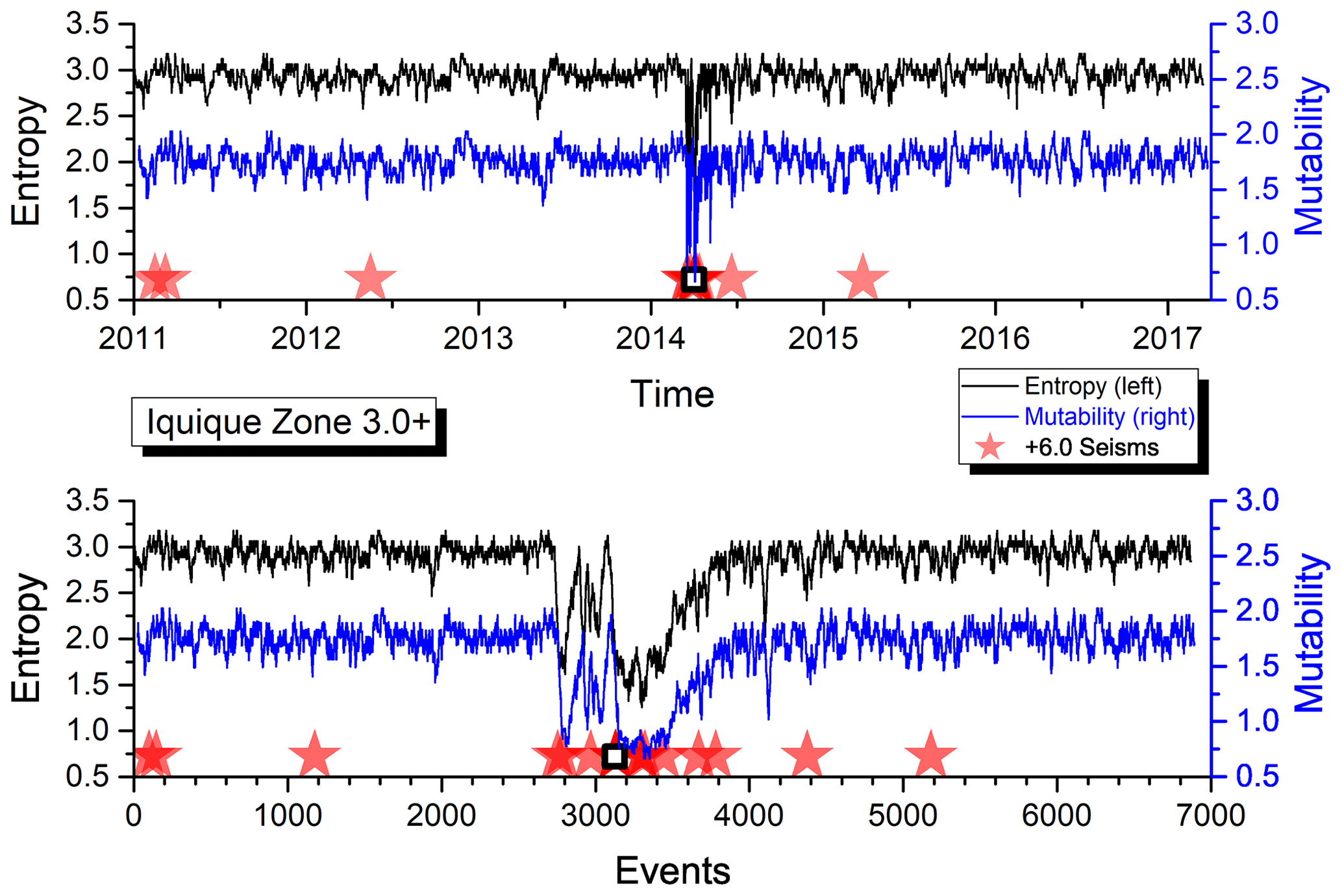
Figure 3Shannon entropy and mutability as functions of time for the seismic activity of zone A. The open star marks the position of the earthquake identified in Table 1. The abscissa in the upper panel corresponds to real time ti, while in the lower panel it represents the natural time of successive events (filtered seisms) denoted by the order label i (Figs. 4–6 use the same procedure).
2.3 Data recognizer
We use here the same dynamic data window of ν events used for the calculation of Shannon entropy. The weight in bytes of the sequence of ν events beginning at natural time i will be denoted by w(ti,ν). This partial sequence is processed by wlzip producing a new sequence that needs bytes of storage. The relative dynamic information content of this time series of seismic events is known as mutability, which is defined as follows:
where w* is the size in bytes of the compressed dataset associated with the time intervals Δj within the time window of ν events.
As already pointed out, ν equals 24 for all mutability calculations below. The typical value of w(ti,ν) for the files measured here is 144 bytes, while the values of vary roughly between 100 and 400 bytes, thus leading to variations in mutability. Mutability is a relative measure of the information content present in a file; monotonic sequences give low mutability values, and chaotic sequences (like those emanating from phase transitions) give high mutability values. Its dynamic response is advantageous in detecting information content even when other methods fail; an example of this is the Edwards–Anderson model in which spin glass transitions are revealed by mutability despite magnetization measurements failing (Cortez et al., 2014). To better illustrate this concept, we include an Appendix calculating the mutability of four different sequences of 24 events.
Two comments are in order. First, wlzip uses compressor algorithms to recognize information, but this does not mean that should be less than w(ti,ν). Second, the value of wlzip depends both on the interval distribution but also on the time sequence of the intervals, which has also been used in the natural time analysis of consecutive heartbeat intervals, while Shannon entropy depends only on the distribution (Varotsos et al., 2007). Thus, the sooner a value in the sequence is repeated, the lower the value of μ(ti,ν) is (Vogel et al., 2012; Cortez et al., 2014). This fact marks a difference between these two parameters, as we will see below.
Figures 3–6 present the Shannon entropy (top) and mutability (bottom) for data corresponding to geographical areas A, B, C and D, respectively, according to Table 1 and Fig. 1. The numeric recognition was done for the data files (intervals in minutes between successive seisms) in quaternary basis both for Shannon entropy and mutability. All registers have the same number of digits, filling with zeroes all empty positions prior to the first significant digit. The matching to recognize the same data register started at position four and was done for three digits including the fourth position (Vogel et al., 2017a). All zones were treated with the same precision.
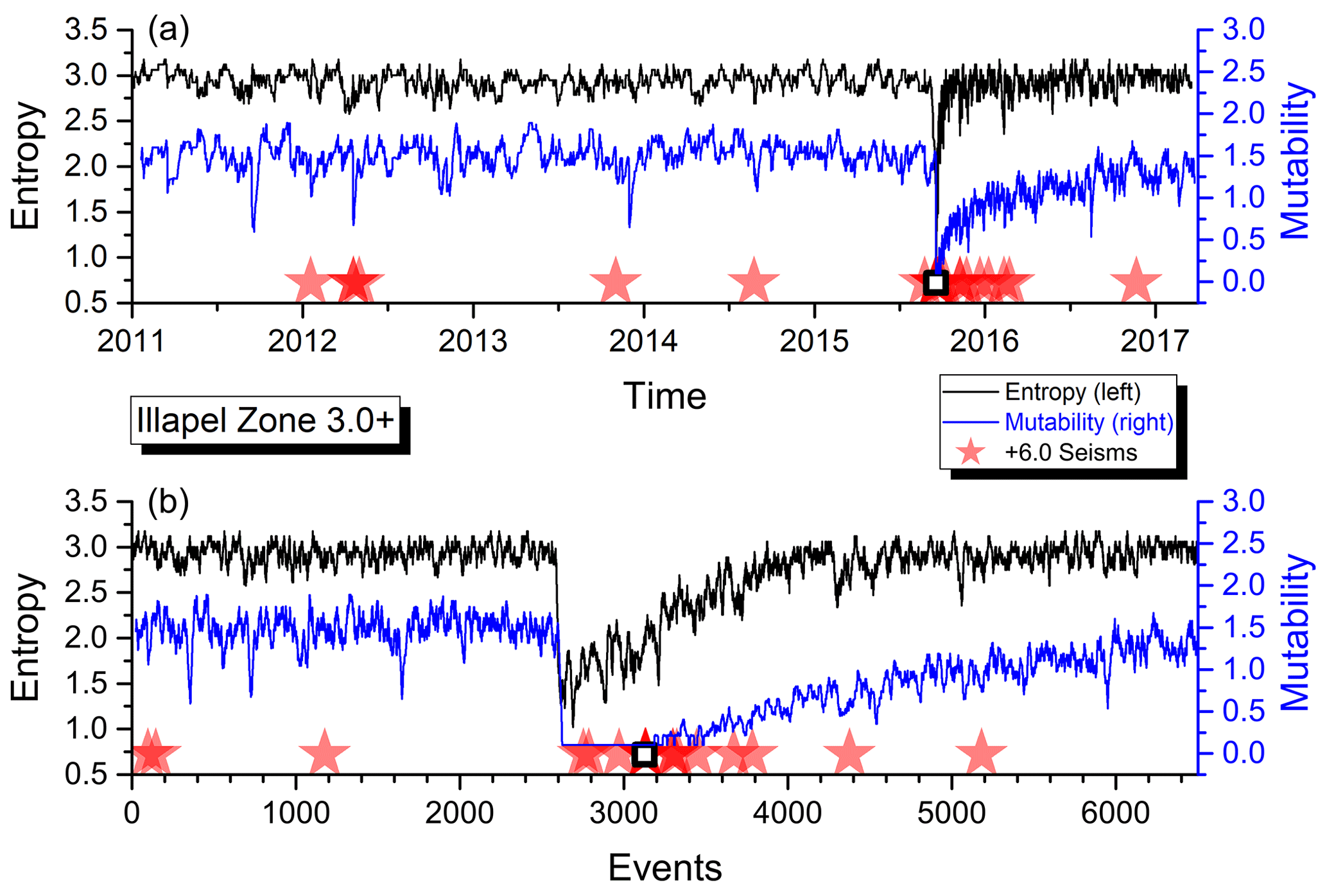
Figure 4Shannon entropy and mutability as functions of real time (a) and natural time (or sequence of events, b) for the seismic activity of zone B. The open star marks the position of the earthquake identified in Table 1.

Figure 5Shannon entropy and mutability as functions of real time (a) and natural time (or sequence of events, b) for the seismic activity of zone C.
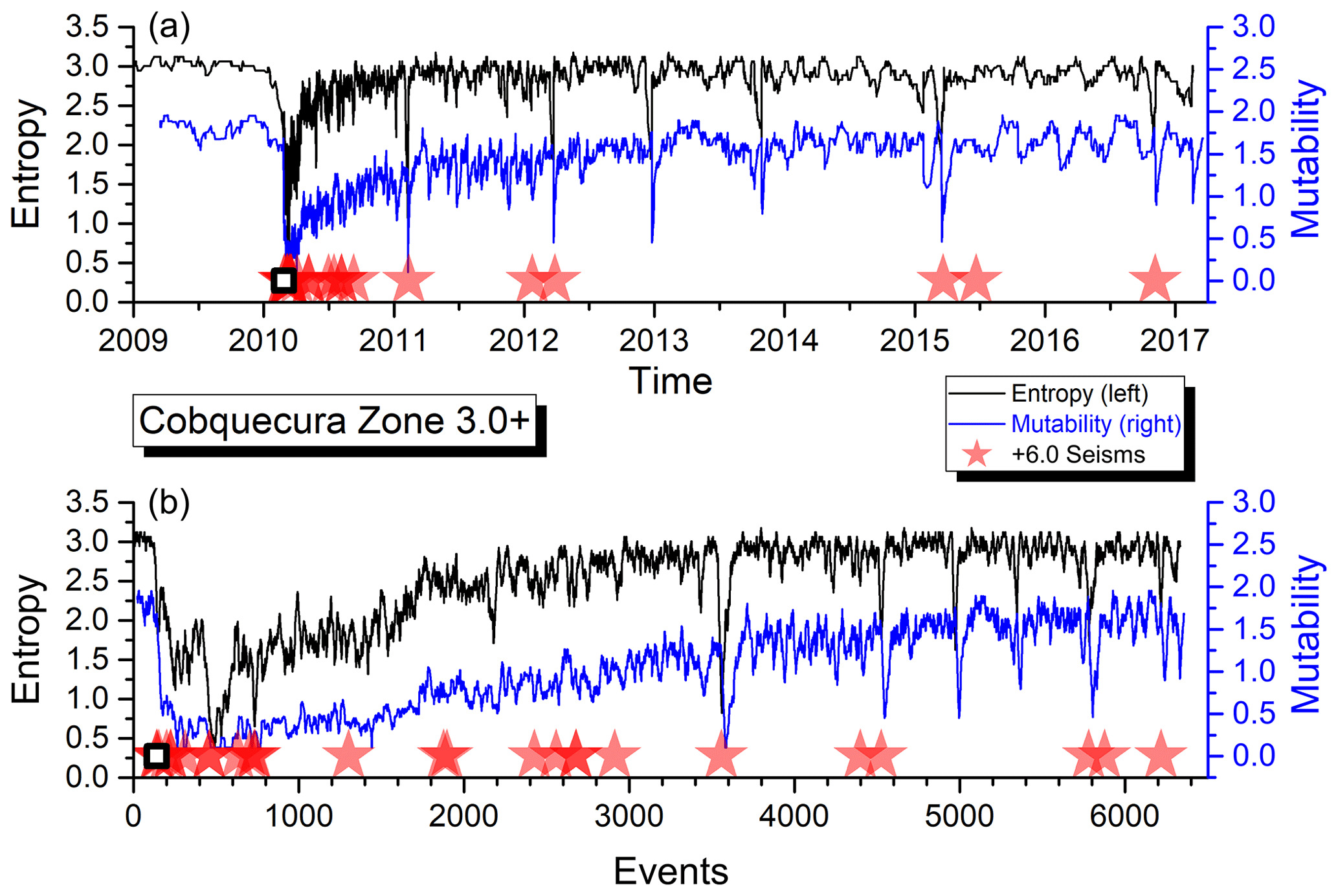
Figure 6Shannon entropy and mutability as functions of real time (a) and natural time (or sequence of events, b) for the seismic activity of zone D. The open star marks the position of the earthquake identified in Table 1.
In the upper panel, the abscissa “Time” corresponds to real time ti (as defined in Sect. 2.2) beginning on 1 January 2011 for zones A, B and C and on 1 January 2009 for zone D. In the lower panel, the abscissa labeled “Events” now corresponds to the succession of filtered seisms identified by the same label i used to define ti. The ordinates are the same in both panels.
In the upper panel, the aftershock behavior is concealed by the large activity in the short time after a large quake, while in the lower panel, it is easier to see the aftershock sequence, although the large quiet periods now look more compressed. Earthquakes over a certain magnitude (as given in the inset for each zone) are marked by a star. The empty square (A, B and D only) identifies the largest earthquake with a magnitude greater than Mw=8.0 within that area as listed in Table 1.
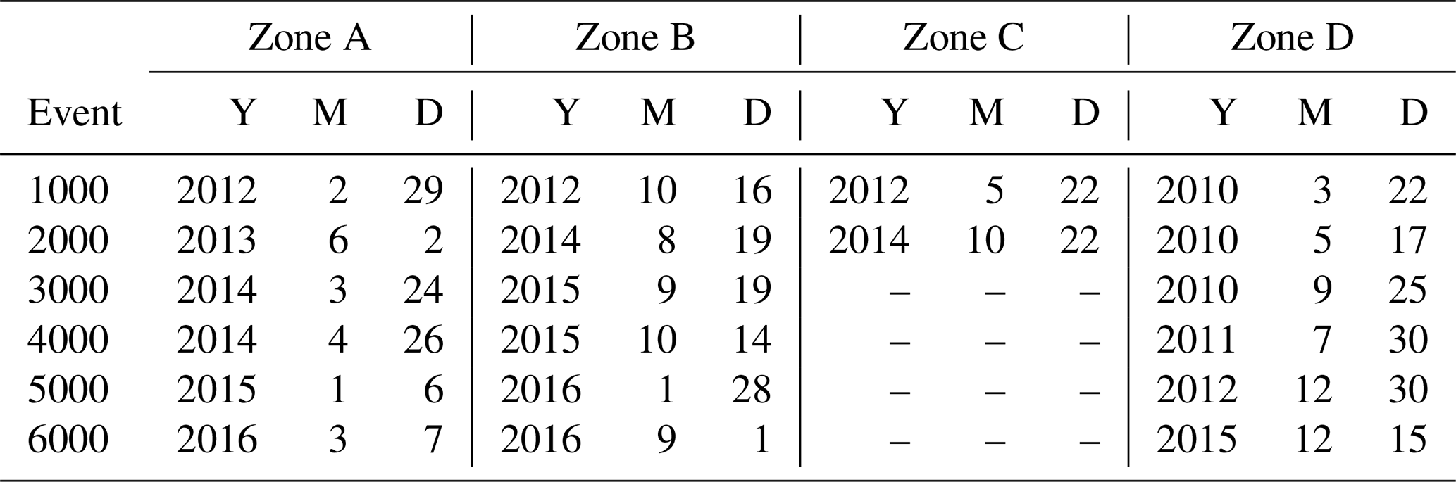
To facilitate the interpretation of these figures and the interrelation between both abscissa axes in each figure, Table 2 interprets the actual real time for the milestone events for the four zones. The date is given by year (Y), month (M) and day (D).
Table 2Equivalence of the milestones for natural time in thousands of events in terms of real date: year (Y), month (M) and day (D) for Figs. 3–6.
As can be observed, both H and μ present a similar behavior for the data in the four areas. Immediately after a large shock, both indicators sharply decrease due to the short intervals between consecutive aftershock quakes thereafter.
The average activity level is relatively constant before a major earthquake and later on after the aftershocks have disappeared. However, such an activity level is not the same for all the areas, which is an indication of different responses to similar phenomena which deserves particular attention, and it will be further investigated below.
To better appreciate the correlation between H and μ, we study the out-of-phase correlations defined as follows:
where ℓ is the phase difference measured in terms of the number of events separating the measurement of one parameter with respect to the other, and m=50 is the range or maximum phase difference in either sense considered here. This value is entirely empirical and looks for flat behavior of previously defined correlations. From Fig. 7, it may appear that m=30 could be enough, but we decided to explore a bit further to make sure curves are already tending to a flat behavior. Previous equations represent the average over the possible equivalent ranges within the series of N registers. In addition, σH and σμ represent the standard deviations of H and μ through the N events, respectively.
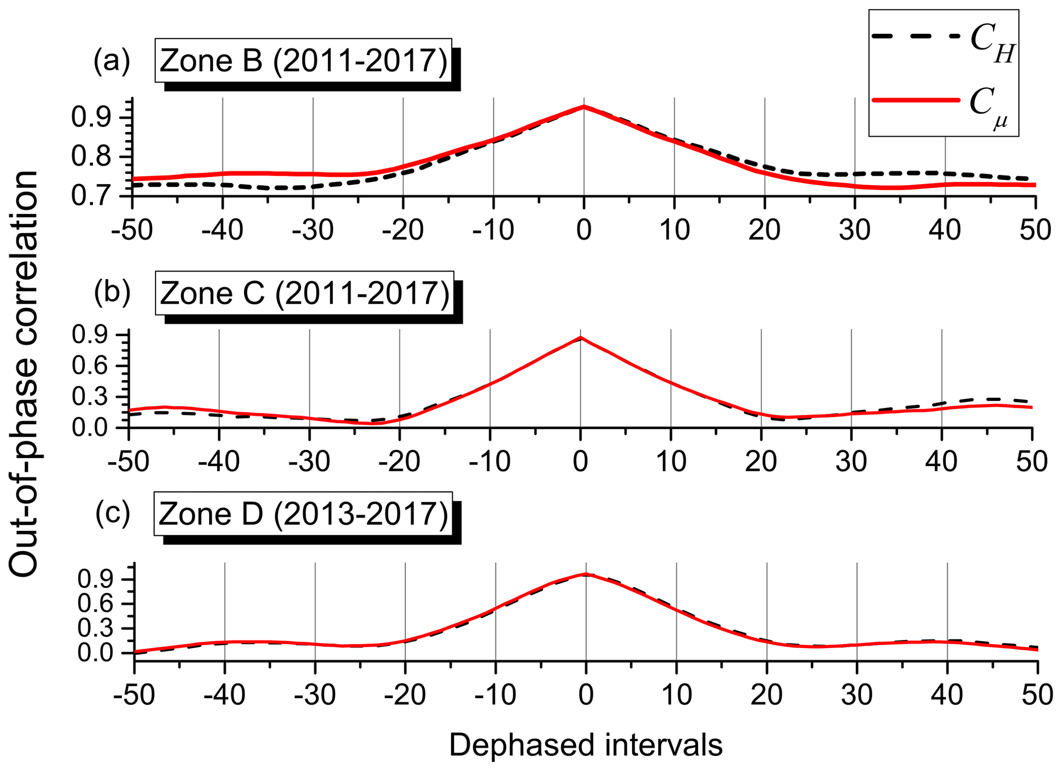
Figure 7Out-of-phase correlations. (a) Zone B data including the aftershock regime (similar ones are obtained for zones A and D with aftershock regimes). (b) Zone C data that does not present an aftershock regime. (c) Truncated zone D data excluding the aftershock regime.
The out-of-phase correlation between Shannon entropy and mutability is presented in Fig. 7. It was found that in general the full correlation is lost after about 20 events. A general prevalence is observed in the form of a tendency towards a constant behavior far from the maximum: a value around 0.75 in the wings of zone B (Fig. 7a) and towards 0.15 for zone C (Fig. 7b). Similar figures were analyzed for zones A and D with prevalence values near 0.75 and 0.57, respectively. To test if these prevalence correlations are due to the aftershock regimes, a reevaluation of the out-of-phase correlation was done for zone D that was restricted to results of Shannon entropy and mutability obtained after 1 January 2013, thus diminishing the effect of the aftershock regime; these results are also shown in Fig. 7c. So the main correlation between Shannon entropy and mutability is obtained during the aftershock period. On the other hand, the out-of-phase correlations tend to be completely lost during periods without the influence of this regime. This is a first indication of partial independence between Shannon entropy and mutability.
The recovery of the activity level after a major earthquake is faster for the Shannon entropy than for the mutability. Namely, the slope in the recovery for μ is better defined after a large quake. It is interesting to notice from Figs. 3 through 6 that zone A recovered its foreshock activity level sooner than any of the other zones. This observation will be put in a quantitative way concentrating on the recovery dynamics in real time to compare the behavior of the different zones.
Figure 8 presents the mutability results for zone D starting at the point of minimum mutability occurring immediately after the major earthquake on 27 February 2010. The dotted (red) curve corresponds to an exponential fit to be discussed next. The inset shows the same data and exponential adjustment for the first 2 years of the time span. A power law can be seen at the onset of the aftershock regime resembling Omori's law.

Figure 8Exponential fit for the Cobquecura dataset after 27 February 2010. This dataset starts at the point of minimum mutability after the big earthquake of magnitude Mw=8.8.
For zones A, B and D, we assume an exponential adjustment of the mutability function after the largest earthquake. A possibility of such a function is the following:
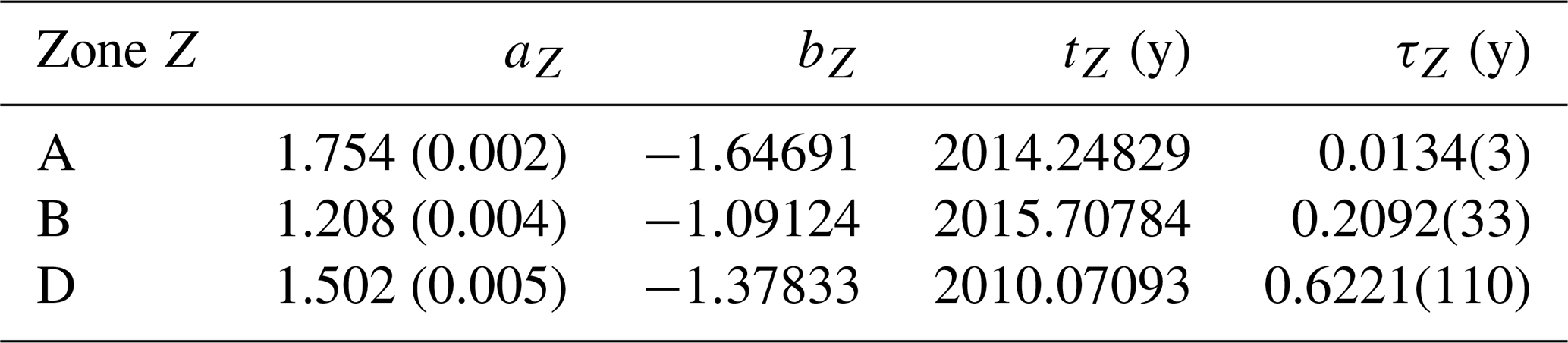
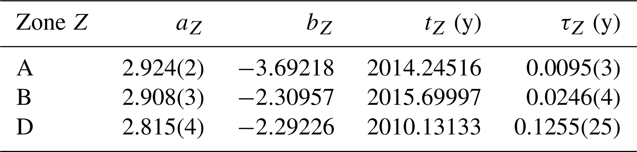
where aZ measures the “asymptotic” activity of zone Z (reached after the aftershocks regime), tZ corresponds to the time of minimum mutability after the largest earthquake (Table 1) and serves as initial time for this recovery analysis, τZ is the characteristic time for activity recovery in zone Z, and bZ is just a shape adjustment parameter without a direct meaning for this analysis.
For zone D (Fig. 8), the best least square fit for the mutability is obtained for aD=1.502(2) and τD=0.62212 years. The results of this treatment for all the zones with major earthquakes are summarized in Table 3. Figure 8 includes an inset with a semilog scale to appreciate the recovery process from a different perspective. A linear behavior in this scale is apparent at the beginning of the plot, but then it is rapidly lost. The sudden decrease in mutability values during February 2011 is better resolved in the timescale of the inset; this is due to the short aftershock activity produced by the earthquake of magnitude 6.1 occurring on 14 February 2011. Due to their sharp appearance, we propose the name “needles” for these sudden and short decreases in mutability associated with the brief aftershock period produced by seisms of Mw=5.0 to Mw=6.0 approximately. Other needles can be easily spotted in Figs. 3–6 and 8.
Table 3Best fit parameters for the mutability of zones A, B and D after the main earthquake using the exponential trial function given by Eq. (6).
A similar analysis was made for the Shannon entropy results using the same exponential fit, and the corresponding parameters are given in Table 4.
Table 4Best fit parameters for Shannon entropy of zones A, B and D after the main earthquake using the exponential trial function of Eq. (6).
Figures similar to Fig. 8 were made for the mutability of zones A and B using the best fit parameters listed in Table 3. The same analysis was also done for the results obtained by Shannon entropy, and the corresponding parameters are given in Table 4. The figures backing such fittings are not included here since they are very similar to Fig. 8 and the procedure is the same to the one already established in the presentation of this figure.
Let us now discuss the results given in Tables 3 and 4, which list the parameters defined in Eq. (6). The first striking difference between Shannon entropy and mutability is in the value of the background parameter aZ. In the case of the adjustment for Shannon entropy, this parameter does not discriminate significantly among zones with values close to 2.9 for all of them; the same parameter in the case of the mutability data spans a range of [1.208,1.754], thus indicating differences in the dynamics of these three regions. In particular, mutability indicates that in zone B, there are more seismic events at regular intervals than in the other zones. Given the underlying plate subduction mechanism, this could mean that plates are sliding more regularly or even fluently in zone B, whereas the relative motion of the Nazca plate under the South American plate is more difficult in zone A, thus leading to more disperse set of intervals between consecutive seisms.
After a large earthquake, the zones tend to recover their characteristic activity level aZ, but this is done rather abruptly for Shannon entropy, while it is more gradual for mutability. This is measured by the recovery time τZ in Tables 3 and 4. In the case of the Shannon entropy for zone A, the recovery is very fast, namely 0.00947 years ≈3.5 d. In the case of zones B and D, the recovery times for the Shannon entropy are 9 and 45 d, respectively. However, when the analysis is done using the recovery time for mutability (Table 3), the recovery times are 5 d, 2.5 months and 7.5 months for zones A, B and D, respectively.
Tables 3 and 4 also show that recovery times τZ are different, being shorter for Shannon entropy and longer for mutability, but the tendencies are the same. So eventually both methods can be used to characterize this aspect of the aftershock regime. In terms of the human perception experienced after any large earthquake, it seems that τZ values obtained for the mutability results are more representative of the aftershock times experienced in each zone. Thus, for instance, seisms of magnitudes around 4.0 were frequent in zone D for several months after 10 February 2010, but this was not the case for zone A where people could not perceive the aftershock regime after a week or so of the last earthquake in this area.
The main difference between Shannon entropy and mutability is that the former analyzes the distribution of registers in a sequence regardless of the order in which these entries were obtained, while the latter gives a lower result for sequences including frequently repeated registers (Cortez et al., 2014). Shannon entropy considers the visit to a state without considering the order in which these visits take place, which is of paramount importance for the entropy in natural time being dynamic entropy and not static (Varotsos, 2005; Varotsos et al., 2007), so it pays exclusive attention to the probability of visiting a state at some instance during the observation time. Mutability also considers the trajectory in which these visits take place, giving lower results when the system stays long periods in the same state or states directly connected to this state; in contrast, during agitated periods (chaotic dynamics would be at the apex here), mutability gives higher results. In other words, a given sequence has just one result for Shannon entropy, but the permutations of the order of the registers lead to different results for mutability; in the present case, the mutability results reported here correspond to the natural sequence of the recorded seisms.
We now focus on the analysis of the background activity obtained for the four zones described in this work by taking semestral averages of the values of mutability in Figs. 9–12 in order to study trends in timescales longer than the one of previous figures. We have chosen a semester as the time for averages, so we have a few hundred registers in each partial sequence minimizing error, but still we have some 13 points in the overall period to appreciate tendencies and differences. In doing so, we also evaluate semestral averages of intervals between consecutive seisms, which show similar trends to the mutability results for the same period.

Figure 9Semestral average of mutability values (upper symbols; black) and intervals in minutes between consecutive seisms (lower symbols; blue) for zone A (Iquique). Odd semesters are labeled on the abscissa axis (1–13; first semester of 2013), while even semesters are only marked. A star identifies a semester with an earthquake with a magnitude over 8.0.
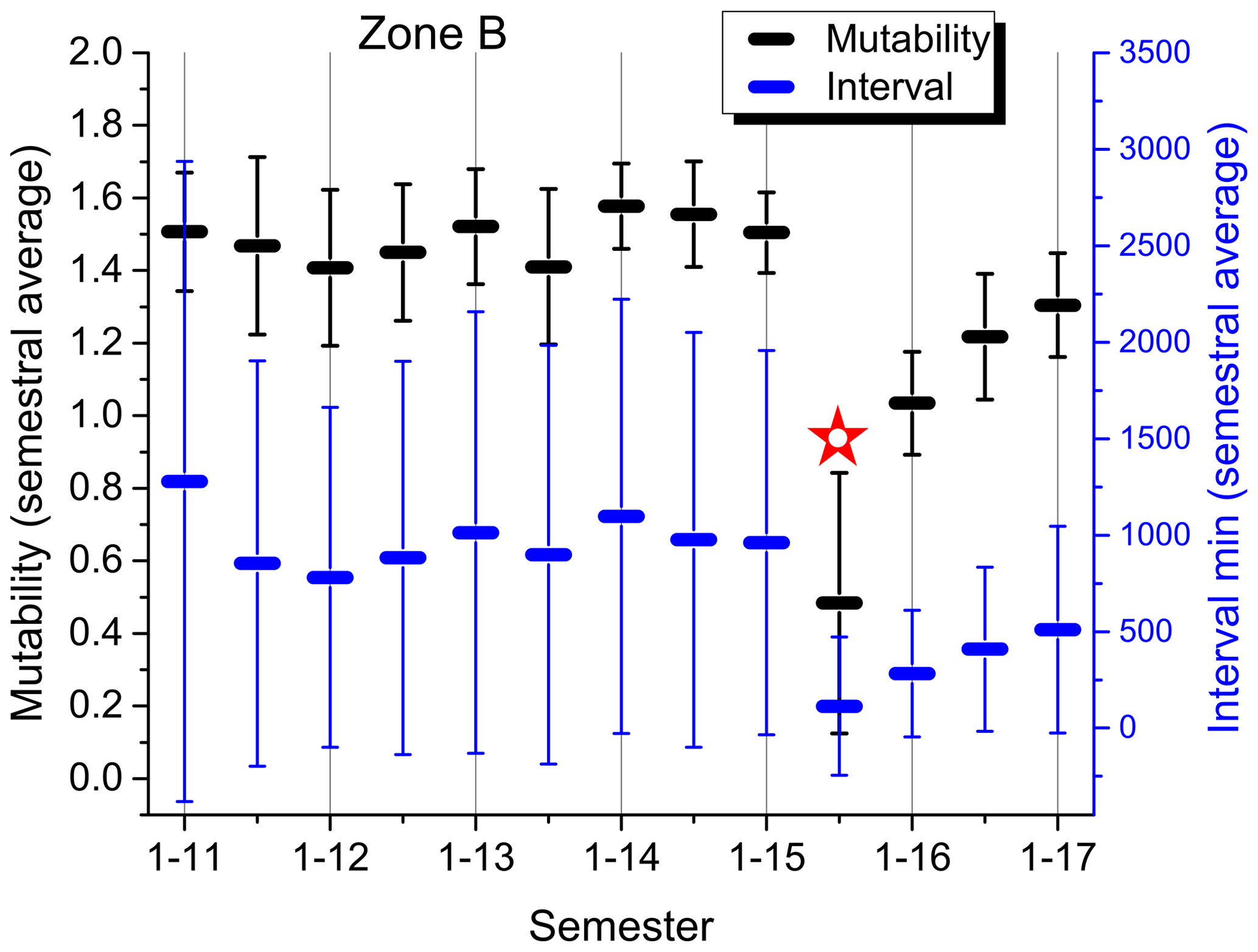
Figure 10Semestral average of mutability values (upper symbols; black) and intervals in minutes between consecutive seisms (lower symbols; blue) for zone B (Illapel). Odd semesters are labeled on the abscissa axis (1–13; first semester of 2013), while even semesters are only marked. A star identifies a semester with an earthquake with a magnitude over 8.0.
The semestral analyses for zones A, B, C and D are shown in Figs. 9–12, respectively; they are all presented under the same scale to allow a direct comparison. The mutability values run on the upper part (black), while the intervals tend to occupy the lower part (blue) of the plot. The first comment here is evident: these four regions present different responses to the evaluation of their sequences of time intervals between consecutive seisms of magnitude 3.0+ as measured both by mutability and Shannon entropy. These two measures are not equivalent either, although some general similarity between them can be noticed. The only effective common feature is that an earthquake with a magnitude over 8.0 produces an absolute minimum for each variable during the semester containing this seism and its aftershock sequence.
For didactic reasons, we shall perform this discussion beginning with zone D, where the long recovery period already noted in Fig. 12 and in Table 3 is more enhanced. It is interesting to observe that the average semestral mutability presents recent relaxations like in the first semester of 2015 and the first semester of 2017. Generally speaking these results do not approach each other, yet the values are near 1.8 for the average semestral mutability in the foreshock period preceding the large earthquake of 2010. Interval semestral averages tend to follow the variations of mutability, but some differences are noticed. The present average interval of about 2000 min (about 33 h) is far from the almost 6000 min interval before the large earthquake.
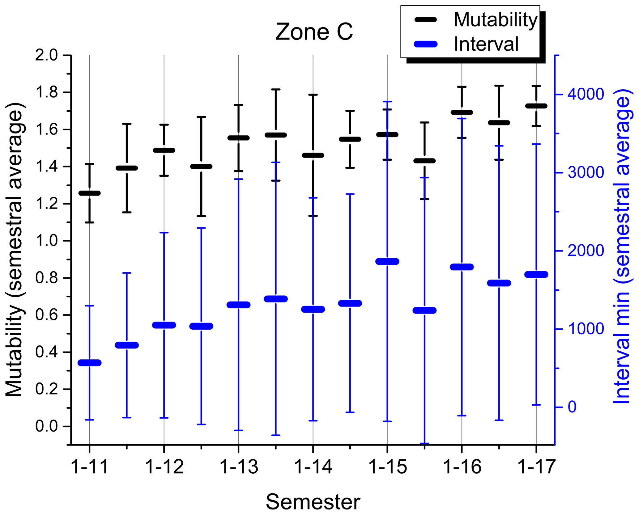
Figure 11Semestral average of mutability values (upper symbols; black) and intervals in minutes between consecutive seisms (lower symbols; blue) for zone C (calm). Odd semesters are labeled on the abscissa axis (1–13; first semester of 2013), while even semesters are only marked.
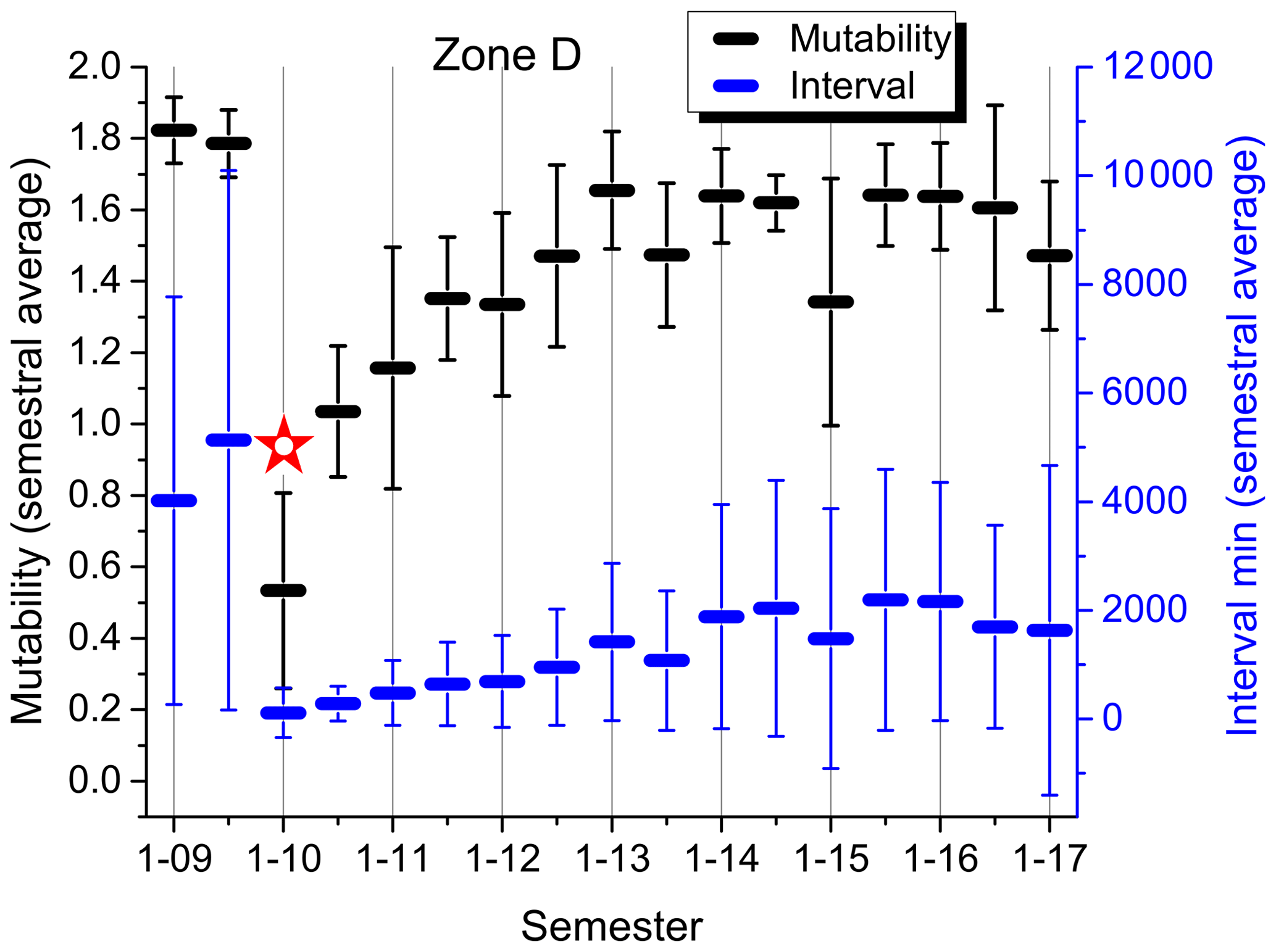
Figure 12Semestral average of mutability values (upper symbols; black) and intervals in minutes between consecutive seisms (lower symbols; blue) for zone D (Cobquecura). Odd semesters are labeled on the abscissa axis (1–13; first semester of 2013), while even semesters are only marked. A star identifies a semester with an earthquake with a magnitude over 8.0.
Figure 11 is completely different to the others. There is no major earthquake included here, but it is obvious that there was one prior to 2011 from which this activity is slowly recovering. The general tendency is to slowly increase the mutability values to levels similar to those constantly presented by zone A and those presented by zone D prior to the large earthquake. Interval averages also increase reaching just under 2000 min. If this is an announcement for a future major earthquake in zone C or nearby, it is still too early to tell, but this zone should be monitored closely.
Figure 10 shows the foreshock mutability averages for zone B, which present a nearly flat behavior around 1.6 before the major earthquake of 2015. Then, after the aftershock regime, the average semestral mutability begins to recover faster than in zone D but still not reaching the level shown here prior to the large earthquake. The observation is similar for the interval semestral average whose value is still small compared to the activity before 2016.
Figure 9 shows the almost constant results (near 1.8) for the average semestral mutability of zone A with just one semester reaching a moderate low value (1.4 with a large error bar). The semestral average for intervals between seisms is also rather flat around 10 h. The only exception is the first semester of 2014 coinciding with the large earthquake there.
Error bars deserve a separate discussion. They are obtained from the standard deviations calculated for the distributions of each semester within each zone. So the number of events differs from one semester to another even within each zone. In the case of intervals, the largest semestral error is 4966 min for zone D during the second semester of 2009, just prior to the large earthquake of 2010. The smallest error is 280 min obtained for the first semester of 2014, which includes the large earthquake and related activity in zone A. In the case of mutability, its largest semestral error is for zone A during the first semester of 2014, while the smallest one is during the second semester of 2013 for this same zone. So error bars are subject to some fluctuations also, but still they are a general indication of the homogeneity of the data.
Mutability error bars are rather small for zone A, meaning that the intervals are rather similar along the data sequence. This is reinforced by the average interval error bars which are the smallest among the four zones (spanning only about 1200 min), indicating that intervals are not so different among themselves. The largest error bars both for mutability and intervals are to be found in zone D; moreover, they are irregular in recent years. The average of the error bars increased in zone D during 2009 just prior to the huge quake of 2010. However, for this same zone, the corresponding error bars for the average semestral mutability are among the smallest to be found prior to this large earthquake. Once again, it is difficult to say something about the present status of zone B since it is clearly under recovery. However, the calm zone C clearly shows a tendency: error bars for mutability averages are shrinking, while error bars for intervals are growing, spanning about 60 h. These two symptoms were present in zones A, B and D prior to their large respective earthquakes. In the case of zone A, the error bars for the average intervals are not so large, but here is where we find the highest values for mutability and the smallest error bars for this variable.
If we look for common features just before a large earthquake, they are relatively high mutability values (“high” needs to be defined for each zone) and very small error bars associated with semestral mutability averages. The particular values of these indicators for zone A could be interpreted here as an irregular subduction with no short time accommodations or lack of fluency, leading to seismic risk of some sort, although it is not possible to specify any possible time for a large seism in the future. From this point of view, the earthquake of 2014 near Iquique was just a small accommodation of the plates, but the subduction process could be somewhat stuck to the similar levels presented before the large quake.
Seismic activity is different for the four zones defined here along the Nazca–South American subduction trench (Figs. 1 and 2, Table 1). Nevertheless, some general behaviors are common to the seismicity of the tectonic activity present in this region. Both Shannon entropy and mutability show a sudden decrease after an earthquake of a magnitude around or over 7.0 (Figs. 3–6). Additionally, Shannon entropy and mutability reach “high” values before a major earthquake; the scale to define high needs to be tuned to each geographical region and observation time window.
A short time correlation exists between Shannon entropy and mutability during the aftershock regime. However, this correlation is lost far from this regime, thus providing independent tests to characterize the seismic activity (Fig. 7).
The aftershock regime is characterized by successions of low and medium intensity seisms at short intervals producing low values of both Shannon entropy and mutability. After some recovery time, the intervals tend to go back to the kind of intervals present before the large quake. This recovery behavior can be described by exponential adjustments (Fig. 8) which indicate that the characteristic times are longer for mutability than for Shannon entropy (Tables 3 and 4); eventually this speaks in favor of the former to continue the analysis. Another advantage of mutability is that the parameter reflecting the background activity spans larger ranges than the one presented by the adjustment of Shannon entropy (Tables 3 and 4). From these results, the mutability recovery time τZ for zone A lasted a few days, while the same parameters for zone D lasted several months, which is close to the human perception in these zones.
The differences between Shannon entropy and mutability evident after the recovery time are due to the handling of a static distribution by the former, while the latter considers the order in which registers entered in the distribution in accordance with the concept of natural time. The differences between Shannon entropy and mutability evident after the recovery time are due to the handling of a static distribution by the former, while the latter considers exact or approximate repetitions in the data chain. From this point of view, mutability carries more information than Shannon entropy despite both being obtained from the same sequences.
The background activity based on mutability aZ (Tables 3 and 4) is quite different for each zone (Figs. 9 and 10). This means that the subduction process finds different difficulties in each zone. However, some general features describing the motion of the Nazca plate under the South American plate should be present along the trench. To investigate this possibility, we considered semestral averages of mutability values.
Semestral averages for mutability recovered quickly for zone A after the 8.2 earthquake, which indicates that the short intervals after a major earthquake were mostly absent here. Soon, the regime with longer and different intervals reappeared, raising the values of mutability and narrowing the corresponding error bars; this could be interpreted as a warning for a possible earthquake in this zone sometime in the near future. On the opposite side is zone D where the semestral averages still have not recovered to the levels prior to the large 8.8 earthquake of 2010; moreover, there have been instances lowering the semestral averages for mutability with large error bars in recent times, providing evidence of short intervals that indicate activity in a rather continuous way. In the case of zone B, the recovery is still under way, so it is too soon to say anything at this time. Generally speaking, we can observe that mutability values were high and their error bars were small just before a major earthquake in zones A, B and D.
Semestral averages for intervals between consecutive seisms and their corresponding error bars are very different among the different regions. Both values decrease during the aftershock regime, but no clear trend could be found prior to a large earthquake.
As for the calm zone C, the mutability semestral averages are clearly increasing and reaching 1.8 with narrowing error bars. Although each zone can have different thresholds for the triggering of a major event, such a value or slightly lower ones have been present just before large earthquakes in the other zones. Zone C is showing a behavior that should be further studied in the expectation of future large quakes.
Let us close by answering the five points raised in the Introduction, thus summarizing previous discussions and conclusions. (1) Both Shannon entropy and mutability give similar responses to a major earthquake and its immediate aftershock period; however, they are independent and non-correlated during the quieter periods. (2) Shannon entropy deals with the distribution as a whole, while mutability and the entropy defined in natural time (which is dynamic and not static; Varotsos et al., 2007) deal with a sequential distribution of intervals of natural time; this allows the latter to be more effective in providing larger contrasts of the values of the characteristic parameters. (3) The recovery time and background activity are very well characterized by mutability allowing us to discriminate among different zones. (4) The mutability semestral averages reflect the seismic activity of the different zones, indicating where the subduction is relatively fluent or where the process could be stuck. (5) A combined analysis points to zone A as having been stuck for many years and zone C's slowly decreasing fluency in the subduction process, which can be an indication of the accumulation of energy in this zone.
This paper deals with the analysis of an important, but particular, seismic zone, namely the Nazca–South American subduction front. Our results show that the use of mutability and Shannon entropy may distinguish the different dynamics within this trench and, especially, the fact that mutability may give a clue to the recovery time in a given region between major earthquakes. Certainly, further studies should be made in order to establish the general applicability of this approach, by studying both other seismic zones and artificial catalogs, such as those given by the epidemic-type aftershock sequence (ETAS) model. We expect to develop this in future publications.
In this Appendix, we provide examples of the way mutability is calculated following Eq. (3) for time sequences similar to those found in this problem using ν=24, as done dynamically in previous presentations. Each column in Table A1 lists one of these sequences, representing intervals between consecutive seisms in minutes. The first column, called “even”, is monotonic, assigning 1 h intervals evenly. The second column, called “converging”, is constructed by means of two intercalated sequences, one ascending and the other descending, so correlations are diluted. The third column, called “random”, is formed by a randomly generated sequence. The fourth column, called “sequential”, is formed by a monotonic increase in the intervals, so it is highly correlated. As can be readily seen, all columns average around 60 min between consecutive registers.
Results of the mutability of each column are given in the last row. As it could have been anticipated, the even sequence has the least information leading to the lowest mutability value. Next is sequential which reflects a monotonic increase in the time intervals. Markedly higher is converging, for which correlations are poor. The highest mutability value is for the random sequence despite a few values being repeated; if no repetitions are present and/or the interval span is higher, the mutability value would be even larger.
It can be noticed that even in a sequence of 24 events, mutability values can span an order of magnitude, This is even more so for real interevent sequences in which intervals can reach several hours (1000 min or more), thus differentiating behaviors of seismic activity.
Table A1Example of four time sequences (second to fifth columns) averaging 60 min between consecutive events. Mutability values for each column are given in the last row. The first column lists the sequence.

The seismic datasets are freely available to the public and can be downloaded from the website of the Centro Sismológico Nacional http://csn.uchile.cl (University of Chile, 2019).
FB did the main numerical analysis and was involved in editing the paper and in scientific discussions for the whole text. VM and DP were involved in writing and editing the paper and in scientific discussions for the whole text. AC and RM were involved in preparing the background material, editing the paper and participating in the scientific discussions for the whole text. EV was involved in the creation of the numerical code, in editing the paper, and in coordinating the scientific discussions for the whole text. All authors read and commented on the text of the paper at all stages.
The authors declare that they have no conflict of interest.
Eugenio E. Vogel is grateful for partial support from FONDECYT (Chile) under contract 1190036 and the Center for the Development of Nanoscience and Nanotechnology (CEDENNA) funded by CONICYT (Chile) under contract AFB180001. Denisse Pastén thanks the Advanced Mining Technology Center (AMTC) and acknowledges support from FONDECYT grant 11160452. Víctor Muñoz is thankful for support from Fondecyt projects 1161711 and 1201967. Rodrigo A. Miranda acknowledges support from FAPDF (Brazil).
This research has been supported by the FONDECYT (Chile) (grant no. 1190036) and the CEDENNA (Chile) (grant no. AFB180001).
This paper was edited by Oded Katz and reviewed by two anonymous referees.
Altamimi, Z., Collilieux, X., Legrand, J., Garayt, B., and Boucher, C.: A new release of the International Terrestrial Reference Frame based on time series of station positions and Earth Orientation Parameters, J. Geophys. Res., 112, B09401, https://doi.org/10.1029/2007JB004949, 2007.
Bressan, G., Barnaba, C., Gentili, S., and Rossi, G.: Information entropy of earthquake populations in northeastern Italy and western Slovenia, Phys. Earth Planet. In., 271, 29–46, 2017.
Cakmur, R. V., Egolf, D. A., Plapp, B. B., and Bodenschatz, E.: Bistability and competition of spatiotemporal chaotic and fixed point attractors in Rayleigh-Bénard convection, Phys. Rev. Lett., 79, 1853–1856, 1997.
Chian, A. C.-L., Miranda, R. A., Rempel, E. L., Saiki, Y., and Yamada, M.: Amplitude-phase synchronization at the onset of permanent spatiotemporal chaos, Phys. Rev. Lett., 104, 254102, https://doi.org/10.1103/PhysRevLett.104.254102, 2010.
Contreras, D. J., Vogel, E. E., Saravia, G., and Stockins, B.: Derivation of a Measure of Systolic Blood Pressure Mutability: A Novel Information Theory-Based Metric from Ambulatory Blood Pressure Tests, J. Am. Soc. Hypertens., 10, 217–223, 2016.
Cordaro, E. G., Venegas, P., and Laroze, D.: Latitudinal variation rate of geomagnetic cutoff rigidity in the active Chilean convergent margin, Ann. Geophys., 36, 275–285, https://doi.org/10.5194/angeo-36-275-2018, 2018.
Cortez, V., Saravia, G., and Vogel, E. E.: Phase diagram and reentrance for the 3D Edwards-Anderson model using information theory, J. Magn. Magn. Mater., 372, 173–180, 2014.
Cover, T. M. and Thomas, J. A.: Elements of Information Theory, 2nd edn., John Wiley and Sons, New York, 2006.
Crisanti, A., Falcioni, M., Paladin, G., Serva, M., and Vulpiani, A.: Complexity in quantum systems, Phys. Rev. E, 50, 1959–1967, 1994.
de Arcangelis, L., Godano, C., Grasso, J. R., and Lippiello, E.: Statistical physics approach to earthquake occurrence and forecasting, Phys. Rep., 628, 1–91, 2016.
De Santis, A., Cianchini, G., Favali, P., Beranzoli, L., and Boschi, E.: The Gutenberg–Richter law and entropy of earthquakes: Two case studies in central Italy, B. Seismol. Soc. Am., 101, 1386–1395, 2011.
Klein, E., Duputel, Z., Zigioni, D., Vigny, C., Boy, J. P., Doubre, C., and Meneses, G.: Deep Transient Slow Slip Detected by Survey GPS in the Region of Atacama, Chile, Geophys. Res. Lett., 45, 12263–12273, 2018.
Lippiello, E., Corral, A., Bottiglieri, M., Godano, C., and de Arcangelis, L.: Scaling behavior of the intertime distribution: Influence of large shocks and time scale in the Omori law, Phys. Rev. E, 86, 086119, https://doi.org/10.1103/PhysRevE.86.066119, 2012.
Luenberg, D. G.: Information Science, 2nd edn., Princeton University Press, Princeton NJ, 2006.
Manshour, P., Saberi, S., Sahimi, M., Peinke, J., Pacheco, A. F., and Tabar, M. R. M.: Turbulencelike behavior of seismic time series, Phys. Rev. Lett., 102, 014101, https://doi.org/10.1103/PhysRevLett.102.014101, 2009.
Métois, M., Socquet, A., and Vigny, C.: Interseismic coupling, segmentation and mechanical behavior of the central Chile subduction zone, J. Geophys. Res., 117, B03406, https://doi.org/10.1029/2011JB008736, 2012.
Métois, M., Socquet, A., Vigny, C., Carrizo, D., S. Peyrat, S., Delorme, A., Maureira, E., Valderas-Bermejo, M.-C., and Ortega, I.: Revisiting the North Chile seismic gap segmentation using GPS-derived interseismic coupling, Geophys. J. Int., 194, 1283–1294, 2013.
Miranda, R. A., Rempel, E. L., and Chian, A. C.-L.: On-off intermittency and amplitude-phase synchronization in Keplerian shear flows, Mon. Not. R. Astron. Soc., 448, 804–813, 2015.
Nicolis, O. and Mateu, J.: 2D Anisotropic wavelet entropy with an application to earthquakes in Chile, Entropy, 17, 4155–4172, 2015.
Roederer, J. G.: Information and its role in Nature, 2nd edn., Springer, Heidelberg, 2005.
Rundle, J. B., Luginbuhl, M., Giguere, A., and Turcotte, D. L.: Natural Time, Nowcasting and the Physics of Earthquakes: Estimation of Seismic Risk to Global Megacities, Pure Appl. Geophys., 175, 647–660, 2018.
Rundle, J. B., Giguere, A., Turcotte, D. L., Crutchfield, J. P., and Donnellan, A.: Global SeismicNowcasting With Shannon Information Entropy, Earth Space Sci., 6, 191–197, 2019.
Sarlis, N. V., Skordas, E. S., Varotsos, P. A., Nagao, T., Kamogawa, M., Tanaka, H., and Uyeda, S.: Minimum of the order parameter fluctuations of seismicity before majorearthquakes in Japan, P. Natl. Acad. Sci. USA, 110, 13734–13738, 2013.
Sarlis, N. V., Skordas, E. S., Varotsos, P. A., Nagao, T., Kamogawa, M., and Uyeda, S.: Spatiotemporal variations of seismicity before major earthquakes in the Japanese area and their relation with the epicentral locations, P. Natl. Acad. Sci. USA, 112, 986–989, 2015.
Sarlis, N. V., Skordas, E. S., Mintzelas, A., and Papadopoulou, K. A.: Micro-scale, mid-scale, and macro-scale in global seismicity identified by empirical mode decomposi-tion and their multifractal characteristics, Sci. Rep., 8, 9206, https://doi.org/10.1038/s41598-018-27567-y, 2018a.
Sarlis, N. V., Skordas, E. S., and Varotsos, P. A.: A remarkable change of the entropyof seismicity in natural time under time reversal before the super-giant M9 Tohoku earthquake on 11 March 2011, EPL-Europys. Lett., 124, 29001, https://doi.org/10.1209/0295-5075/124/29001, 2018b.
Sarlis, N. V., Varotsos, P. A., Skordas, E. S., Uyeda, S., Zlotnicki, J., Nagao, T., Rybin, A., Lazaridou-Varotsos, M. S., and Papadopoulou, K. A.: Seismic Electric Signals in seismicprone areas, Earthquake Sci., 31, 44–51, https://doi.org/10.29382/eqs-2018-0005-5, 2018c.
Shannon, C. E.: A mathematical theory of communication, Bell. Syst. Tech. J., 27, 379–423, 1948.
Telesca, L., Lapenna, V., and Lovallo, M.: Information entropy analysis of seismicity of Umbria-Marche region (Central Italy), Nat. Hazards Earth Syst. Sci., 4, 691–695, https://doi.org/10.5194/nhess-4-691-2004, 2004.
Telesca, L., Lovallo, M., Mohamed, A. E. A., ElGabry, M., El-hady, S., Abou Elenean, K. M., and ElBary, R. E. F.: Informational analysis of seismic sequences by applying the Fisher Information Measure and the Shannon entropy: An application to the 2004–2010 seismicity of Aswan area (Egypt), Physica A, 391, 2889–2897, 2012.
Telesca, L., Lovallo, M., Chamoli, A., Dimri, V. P., and Srivastava, K.: Fisher-Shannon analysis of seismograms of tsunamigenic and non-tsunamigenic earthquakes, Physica A, 392, 3424–3429, 2013.
Telesca, L., Lovallo, M., Romano, G., Konstantinou, K. I., Hsu, H.-L., and Chen, C.-C.: Using the informational Fisher-Shannon method to investigate the influence of long-term deformation processes on geoelectrical signals: An example from the Taiwan orogeny, Physica A, 414, 340–351, 2014.
Vallianatos, F., Papadakis, G., and Michas, G.: Generalized statistical mechanics approaches to earthquakes and tectonics, P. R. Soc. A, 472, 20160497, https://doi.org/10.1098/rspa.2016.0497, 2016.
Varotsos, P. and Alexopoulos, K.: Physical properties of the variations of the electricfield of the earth preceding earthquakes, I. Tectonophysics, 110, 73–98, 1984a.
Varotsos, P. and Alexopoulos, K.: Physical properties of the variations of the electricfield of the earth preceding earthquakes, II. Determination of epicenter and magnitude, Tectonophysics, 110, 99–125, 1984b.
Varotsos, P., Alexopoulos, K., Nomicos, K. and Lazaridou, M.: Earthquake prediction andelectric signals, Nature, 322, 120, https://doi.org/10.1038/322120a0, 1986.
Varotsos, P. and Lazaridou, M.: Latest aspects of earthquake Prediction in Greecebased on Seismic Electric Signals. I, Tectonophysics, 188, 321–347, 1991.
Varotsos, P., Alexopoulos, K., and Lazaridou, M.: Latest aspects of earthquake predictionin Greece based on Seismic Electric Signals II, Tectonophysics, 224, 1–37 1993.
Varotsos, P. A., Sarlis, N., and Skordas, E.: Spatiotemporal complexity aspects on the Interrelation between Seismic Electric Signals and seismicity, Practica of Athens Academy, 76, 294–321, 2001.
Varotsos, P. A., Sarlis, N. V., and Skordas, E. S.: Long-range correlations in the electric signals that precede rupture, Phys. Rev. E, 66, 011902, https://doi.org/10.1103/PhysRevE.66.011902, 2002.
Varotsos, P. A., Sarlis, N. V., and Skordas, E. S.: Attempt to distinguish electric signals of a dichotomous nature, Phys. Rev. E 68, 031106, https://doi.org/10.1103/PhysRevE.68.031106, 2003.
Varotsos, P.: The Physics of Seismic Electric Signals, TerraPub, Tokyo, 338 pp., 2005.
Varotsos, P. A., Sarlis, N. V., Skordas, E. S., and Lazaridou, M. S.: Identifying sudden cardiac death risk and specifying its occurrence time by analyzing electrocardiograms in natural time, Appl. Phys. Lett., 91, 064106, https://doi.org/10.1063/1.2768928, 2007.
Varotsos, P. A., Sarlis, N. V., and Skordas, E. S.: Natural Time Analysis: The new view of time. Precursory Seismic Electric Signals, Earthquakes and other Complex Time Series, Springer-Verlag, Berlin Heidelberg, 2011a.
Varotsos, P. A., Sarlis, N. V., and Skordas, E. S.: Scale-specific order parameter fluctuations of seismicity in natural time before mainshocks, EPL-Europhys. Lett., 96, 59002, https://doi.org/10.1209/0295-5075/96/59002, 2011b.
Varotsos, P. A., Sarlis, N.V, Skordas, E. S., Uyeda, S., and Kamogawa, M.: Natural time analysis of critical phenomena, P. Natl. Acad. Sci. USA, 108, 11361–11364, 2011c.
Varotsos, P. A., Sarlis, N. V., and Skordas, E. S.: Phenomena preceding major earthquakes interconnected through a physical model, Ann. Geophys., 37, 315–324, https://doi.org/10.5194/angeo-37-315-2019, 2019.
Venegas-Aravena, P., Cordaro, E. G., and Laroze, D.: A review and upgrade of the lithospheric dynamics in context of the seismo-electromagnetic theory, Nat. Hazards Earth Syst. Sci., 19, 1639–1651, https://doi.org/10.5194/nhess-19-1639-2019, 2019.
Vogel, E. E. and Saravia, G.: Information Theory Applied to Econophysics: Stock Market Behaviors, European, J. Phys. B, 87, 1–15, 2014.
Vogel, E. E., Saravia, G., Bachmann, F., Fierro, B., and Fischer, J.: Phase Transitions in Edwards-Anderson Model by Means of Information Theory, Physica A, 388, 4075–4082, 2009.
Vogel, E. E., Saravia, G., and Cortez, L. V.: Data Compressor Designed to Improve Recognition of Magnetic Phases, Physica A, 391, 1591–1601, 2012.
Vogel, E. E., Saravia, G., Astete, J., Díaz, J., and Riadi, F.: Information Theory as a Tool to Improve Individual Pensions: The Chilean Case, Physica A, 424, 372–382, 2015.
Vogel, E. E., Saravia, G., Pasten, D., and Munoz, V.: Time-series analysis of earthquake sequences by means of information recognizer, Tectonophysics, 712, 723–728, 2017a.
Vogel, E. E., Saravia, G., and Ramirez-Pastor, A. J.: Phase diagrams in a system of long rods on two-dimensional lattices by means of information theory, Phys. Rev. E, 96, 062133, https://doi.org/10.1103/PhysRevE.96.062133, 2017b.
Vogel, E. E., Saravia, G., Kobe, S., Schumann, R., and Schuster, R.: A Novel Method to Optimize Electricity Generation from Wind Energy, Renew. Energ., 126, 724–735, 2018.
University of Chile: Web site of Servicio Sismológico Nacional (Chile), available at: http://csn.uchile.cl (last access: 31 October 2020), 2019.
Xi, H. and Gunton, J. D.: Spatiotemporal chaos in a model of Rayleigh-Bénard convection, Phys. Rev. E, 52, 4963–4975, 1995.
Zhang, Y. and Meng, Q.: A statistical analysis of TIR anomalies extracted by RSTs in relation to an earthquake in the Sichuan area using MODIS LST data, Nat. Hazards Earth Syst. Sci., 19, 535–549, https://doi.org/10.5194/nhess-19-535-2019, 2019.