the Creative Commons Attribution 4.0 License.
the Creative Commons Attribution 4.0 License.
 | 29 Oct 2020
Predictive modeling of hourly probabilities for weather-related road accidents
Henning W. Rust
Uwe Ulbrich
Impacts of weather on road accidents have been identified in several studies with a focus mainly on monthly or daily accident counts. This study investigates hourly probabilities of road accidents caused by adverse weather conditions in Germany on the spatial scale of administrative districts using logistic regression models. Including meteorological predictor variables from radar-based precipitation estimates, high-resolution reanalysis and weather forecasts improves the prediction of accident probability compared to models without weather information. For example, the percentage of correctly predicted accidents (hit rate) is increased from 30 % to 70 %, while keeping the percentage of wrongly predicted accidents (false-alarm rate) constant at 20 %. When using ensemble weather forecasts up to 21 h instead of radar and reanalysis data, the decline in model performance is negligible. Accident probability has a nonlinear relationship with precipitation. Given an hourly precipitation sum of 1 mm, accident probabilities are approximately 5 times larger at negative temperatures compared to positive temperatures. The findings are relevant in the context of impact-based warnings for road users, road maintenance, traffic management and rescue forces.
- Article
(3570 KB) - Full-text XML
-
Supplement
(158 KB) - BibTeX
- EndNote


The road transport system is one of the most complex and dangerous systems that people have to deal with on a daily basis (Peden et al., 2004). In Germany, for example, road accidents led to around 396 600 injuries and 3200 fatalities per year in 2016 (BASt, 2017). Causes for road accidents can be of a technical, behavioral or environmental nature. According to a recent review paper on spatial approaches in road safety studies (Ziakopoulos and Yannis, 2020), variables like traffic volume, speed limit or the number of lanes are frequently considered in accident analyses. Theofilatos and Yannis (2014) show that the impact of weather on road accidents has also been addressed in several studies covering various temporal and spatial scales, focusing on different weather parameters and applying different methods. They find that the effect of precipitation is quite consistent and generally leads to an increased accident frequency. On the other hand, the impact of other weather parameters on road safety is covered by fewer studies and is less consistent.
Two types of studies can be distinguished regarding the temporal scales. One type of study aims to relate road accidents to weather on a monthly or seasonal timescale (e.g., Fridstrøm et al., 1995; Shankar et al., 1995; Eisenberg, 2004; Bergel-Hayat and Depireb, 2004; Stipdonk and Berends, 2008). The aim of these studies is to gain insight into potential policy measures against the effects of adverse weather on road transport (Shankar et al., 1995). Due to the temporal variability of weather on monthly timescales, such studies can only account for aggregated effects by considering for example the number of days with precipitation or the number of days with temperatures below the point of freezing (e.g., Fridstrøm et al., 1995). Other studies focus on daily timescales (e.g., Eisenberg, 2004; Keay and Simmonds, 2005; Caliendo et al., 2007; Brijs et al., 2008). On such timescales, the link between accident counts and the actual weather conditions on a specific day can be established. However, the largest variability of traffic volume and accident rates is observed on subdaily timescales, with peaks during rush hours and low values during night time (Martin, 2002). Weather conditions may also change dramatically within hours. To take into account the combined effect of weather and traffic volume, a subdaily timescale is necessary. Nevertheless, only few studies focus on subdaily timescales (e.g., Hermans et al., 2006a), possibly due to the lack of appropriate data sources. To establish robust relationships between accidents and weather parameters on an hourly timescale, a sufficient number of data are required at a high spatial resolution. However, the analysis of highly resolved accident data is often subject to restrictions due to data protection directives. The spatial scales covered by the different studies vary from the national or state level (Hermans et al., 2006a) down to the level of individual cities (Yannis and Karlaftis, 2010) or specific roads or road segments (Ahmed et al., 2012).
Meteorological data used in accident studies are often derived from measurement stations. Stations are either used individually (e.g., Knapp et al., 2000) or spatially aggregated for the area of interest (e.g., Eisenberg, 2004). In both cases, it is possible that not all relevant weather events are captured because they do not hit a station. Recent studies use radar data to estimate the impact of precipitation on accidents (e.g., Mills et al., 2019). Jaroszweski and McNamara (2014) argue that radar data offer significant advantages over traditional station-based analyses, namely a better representation of rainfall due to a high spatial and temporal resolution.
Different weather parameters with a significant impact on road accidents have been identified. Depending on the study's modeling strategy and the specific formulation of variables characterizing weather, magnitude and even the sign of the weather impact can vary between different studies. The most important weather parameter considered in most studies is precipitation. On wet roads the tire contact force is reduced (Hays and Browne, 1974), which increases the braking distance starting at 100 km h−1 by about 20 % compared to dry roads (Cho et al., 2007). Also glare caused by wet shining surfaces can lead to reduced visibility and increase accident probabilities (Brodsky and Hakkert, 1988). Hermans et al. (2006a) studied hourly accident counts in the Netherlands within a 1-year period and found precipitation to be the most important factor among 17 different variables characterizing weather.
On a monthly basis, snowfall can lead to the reduction in accident numbers, possibly due to indirect effects like reduced traffic volume or the adaption of driving habits (Fridstrøm and Ingebrigtsen, 1991). On the other hand, on a daily basis, the direct effect of snowfall was found to increase the accident risk. For example, Knapp et al. (2000) find that freeway accident rates increase by a factor of 13 in the case of extreme snowstorms. Mills et al. (2019) find that injury and noninjury collisions increase by 66 % and 137 %, respectively, during winter storm events that were characterized by factors like precipitation and low visibility. The winter storm events were identified by using radar- and station-based observations. Malin et al. (2019) observe a sharp increase in relative accident risk if road surface temperatures drop below the freezing point.
Since the first weather impact models for road accidents (Scott, 1986), various types of models have been used in this context. Most popular are generalized linear models (GLMs), e.g., Poisson regression for accident counts or logistic regression for accident probabilities (e.g., Fridstrøm et al., 1995; Caliendo et al., 2007; Keay and Simmonds, 2006), but other methods like state-space (Hermans et al., 2006b) or autoregressive models (Brijs et al., 2008; Scott, 1986; Bergel-Hayat and Depireb, 2004) have also been applied. Mostly, statistical models for weather impact on road accidents are used in an inferential way; they test hypotheses for variable relations by means of statistical hypothesis testing for parameter significance of prescribed predictor variables, also referred to as explanatory modeling (Shmueli, 2010). This contrasts with predictive modeling, where statistical models are used for prediction of yet unobserved instances of the target variable (e.g., accident counts or probabilities). In practice, predictive models are built and assessed using cross-validation.
This study follows the predictive modeling approach: we build and assess the skill of logistic regression models for hourly probabilities of weather-related road accidents at the scale of administrative districts in Germany. The aim is to assess model performance at small spatial and temporal scales as well as identify relevant meteorological predictor variables for optimizing the predictive skill. We thus seek an adequate functional relationship between hourly precipitation and accident probability under different temperature conditions and district characteristics. Instead of station-based observations, we use a gridded radar-based precipitation product and a new high-resolution regional reanalysis. Additionally, using ensemble weather forecasts, we assess the predictive skill of the accident model for lead times of up to 21 h.
Section 2 describes data and preprocessing approaches. Statistical models and associated verification methods are described in Sect. 3. Results of model verification and the application of the models in a case study of a snowfall event are presented in Sect. 4, which is followed by a discussion and conclusions in Sect. 5.
2.1 Accident data
A data set with anonymized information from police reports of all heavy road accidents in Germany from 2007 until 2012 is used (source: Research Data Centre of the Federal Statistical Office and Statistical Offices of the Länder, Statistik der Straßenverkehrsunfälle, 2007–2012, own calculations). Heavy road accidents include all accidents with injuries, fatalities or write-offs. Minor accidents are not included in the data set. In total 2 392 329 accidents were reported during the 6-year period under investigation. Most accidents were indicated by the police as being caused by driver behavior. However, 7.7 % (184 201) of the accidents were indicated as being caused by adverse road conditions, which includes a wet, snowy or icy road but also mud or dirt on the road. This class of accidents, which we refer to as weather-related accidents, is selected to generate the response variable used in the logistic regression models. The location of the individual accidents is available on the level of administrative districts (Landkreise). Because of several territorial reforms during the study period, all accidents are assigned to boundaries of the 401 administrative districts as they existed in 2017. For each district an hourly time series is created, which is one if at least one accident happened within an hour and zero otherwise. In total this results in 21 076 961 data points, of which 0.80 % (168 404) contain at least one weather-related accident.
2.2 Radar-based precipitation data
Gridded hourly precipitation sums derived from the RADOLAN (Radar-Online-Aneichung) data set (Bartels et al., 2004) are available from the German Meteorological Service (DWD) at a spatial resolution of 1 km×1 km. The RADOLAN combines radar reflectivity, measured by the 16 C-band Doppler radars of the German weather radar network, and ground-based precipitation gauge measurements. Because we cannot directly infer the precipitation amount at the ground from radar reflectivity but only the amount of reflection in the lower troposphere, observations from rain gauges are used to calibrate the precipitation amounts estimated from the radar reflectivity in an online procedure typically used for nowcasting. Before calibration, a statistical clutter filtering is applied, and orographic shadowing effects are corrected for. The RADOLAN project aims to combine the benefits of high spatial resolution of the radar network with the accuracy of gauge-based measurements.
2.3 Reanalysis data
A reanalysis produced by a novel convective-scale regional reanalysis system for central Europe (COSMO-REA2; Wahl et al., 2017) is used to generate meteorological predictor variables for the logistic regression models. The reanalysis results from the integration of COSMO-REA2 (a physical model for the atmosphere) with various heterogeneous observational data assimilated. COSMO-REA2 was developed within the framework of the Hans-Ertel-Centre for Weather Research (https://www.hans-ertel-zentrum.de, last access: 28 October 2020). It contains different gridded atmospheric and surface variables for central Europe at a spatial resolution of 2 km and at hourly time steps. Deep convection is explicitly resolved by the model, while shallow convection is parameterized using the Tiedke scheme (Tiedtke, 1989). In addition to conventional station-based observations, radar-derived rain rates are assimilated using latent heat nudging. On hourly to daily timescales, the assimilation of radar information substantially improves the parameterized precipitation compared to other reanalysis data sets (Wahl et al., 2017).
2.4 Ensemble weather forecasts
Weather forecasts are used to study the predictability of accident probabilities based on weather forecasts with an ensemble prediction system (EPS). We use the regional high-resolution ensemble forecasting system COSMO-DE-EPS, which runs operationally at the DWD before May 2018 with a spatial resolution of 2.8 km for the area of Germany. The COSMO-DE-EPS is initiated every 3 h, with a lead time τ of up to 21 h. τ is the difference between the time the model simulation is initialized and the time the forecast is valid for. For example, if the model simulation is initialized at 00:00 UTC, τ=21 h corresponds to the forecast for 21:00 UTC. For each initialization time 20 ensemble members are available, generated using different global model forecasts as initial and lateral boundary conditions and variations in parameterizations for unresolved processes as described in detail in Gebhardt et al. (2011) and Peralta et al. (2012). The spread of the ensemble members allows an estimation of the forecast uncertainty. Similar to COSMO-REA2, precipitation rates derived from radar observations are assimilated at forecast initialization using latent heat nudging (Stephan et al., 2008).
For our study, a postprocessed product of the archived COSMO-DE-EPS forecasts for the years 2011 and 2017 was provided by the DWD. Instead of archiving the forecast data on the original model grid, area averages of 21×21 grid boxes (56 km×56 km) around 758 DWD-owned gauge stations are stored. This drastically reduces the large number of data, which facilitates their processing.
3.1 Data preparation
We aggregate the different meteorological variables to the level of administrative districts. For the station-based COSMO-DE-EPS forecasts a weighted mean of all available stations in the vicinity of the districts was calculated using the probability density function of a bivariate circular symmetric normal distribution as the weighting function. A standard deviation of 25 km proved to be most appropriate as it corresponds well to the average district area.
For a fair comparison of RADOLAN and COSMO-REA2 with COSMO-DE-EPS forecasts, the same aggregation is applied to the gridded RADOLAN and COSMO-REA2 products: the areal averages around the 758 gauge stations are computed as described in Sect. 2.4, and the data are aggregated to the district level by applying the weighting function, as described above.
3.2 Logistic regression
Logistic regression models are used to model the probability of a certain event based on independent predictor variables (e.g., Menard, 2002). Here, we model hourly accident probabilities. If Pt is the probability that an accident occurs in a 1 h time interval , the logistic model equation is
where α is the intercept term, is the set of n predictor variables, and are the corresponding parameters. α and βi are estimated using maximum likelihood. If the effects of the two predictor variables Xti and Xtj are not additive (i.e., the effect of Xti on Pt depends on the state of Xtj), interaction terms can be added to the model equation. If Xti and Xtj are continuous variables, for example, this can be achieved by adding βij Xti Xtj to the linear term in Eq. (1), with βij quantifying the combined effect of Xti and Xtj. For a more detailed description of interactions, see Wood (2017).
The parameters of the logistic regression model can be easily converted to the odds ratio OR=exp βi. The odds ratio for a given term Xti describes the change in the odds that the event will occur in the case of a unit change in Xti.
3.3 Assessing model performance
Parameter estimates associated with individual predictor variables Xti can be tested for being significantly different from 0 using the p values of a two-tailed z test (Dobson and Barnett, 2008).
Different logistic models are compared with information criteria. The most popular is the Akaike information criterion (AIC; Akaike, 1974), defined as
where k is the number of parameters used in the model, and is value of the likelihood at its maximum. Fitted to the same data the model with a lower AIC is to be preferred. The AIC penalizes models with more parameters to prevent overfitting.
The Brier score (BS) is a proper score to measure accuracy of probabilistic forecasts for binary events as they result from a logistic regression model. Based on Brier (1950) the BS can be defined as
where ft is the forecast probability, ot is the observed outcome of the event (), t labels the events, and N is the total number of events. However, Benedetti (2010) has shown that the Brier score may not be suitable when forecasting very rare (or very frequent) events. He suggests the use of the logarithmic score (LS; or absolute score)
where is simply a scaling factor, making LS comparable in size to BS. The LS is frequently used in the field of statistical mechanics and information theory and fulfills three basic desiderata (i.e., additivity, exclusive dependence on physical observations and strictly proper behavior).
By defining a threshold u, a probabilistic forecast () can be transformed into a binary forecast, which is either positive (accident) or negative (no accident) if the forecast probability falls above (f≥u) or below the threshold (f<u), respectively. The true positive rate (TPR, or hit rate) is the number of correctly predicted positive events divided by the total number of positive events. The false positive rate (FPR, or false-alarm rate) is the number of incorrectly predicted negative events divided by the total number of negative events. The receiver operating characteristic (ROC) curve is a common way to illustrate the performance of a logistic regression model as a binary classifier by plotting the TPR against the FPR for various thresholds (Hanley and McNeil, 1982). The area under the ROC curve (AUC) is frequently used for measuring the ability of a model to discriminate between positive and negative events. The AUC ranges between 0.5 and 1, which compares to random guessing and perfect discrimination, respectively. For a given FPR the corresponding TPR can be identified based on the ROC curve. In this study, we compare the TPR of different models while selecting u so that the FPR is kept constant at 0.2.
A skill score SS is a relative measure of how much a forecast Sf outperforms a reference forecast Sr, defined as
where Sp is the score of a perfect forecast. In this study we use the BS to compute the Brier skill score (BSS; ), the LS to compute the logarithmic skill score (LSS; ) and the AUC to compute a skill score based on the ROC curve (AUCSS; ).
Cross-validation is a technique where the performance of a statistical model is tested using independent data that have not been used for estimating the model coefficients. Here, we use a yearly cross-validation approach. Model parameters are estimated on a data set with 1 year of data left out, and scores are calculated for this respective year. This is repeated several times until a score has been estimated for all years. The score is then averaged over all years and used for model comparison.
To understand the behavior of the model, the predicted accident probabilities of the regression models can be compared to nonparametric estimates for accident frequencies within bins of specific parameter ranges. For example, a predicted accident probability for negative temperatures and a precipitation amount of 1 mm h−1 at 07:00 local time can be compared to the relative accident frequency for all time steps that showed negative temperatures and precipitation amounts in an interval of 1±0.1 mm at 07:00. The uncertainty of model probability forecasts is estimated by computing the 95 % confidence interval based on asymptotic standard errors. The uncertainty related to the nonparametric estimates of the accident frequency is estimated by using a bootstrapping approach. The observed accident frequency is computed 10 000 times after drawing random samples with replacement from the available data. The range between the 0.025 and 0.975 quantile of the resulting distribution of values can be used to construct a 95 % confidence interval around the average observed accident frequency.
3.4 Model description
3.4.1 Models without weather information
The models NULL and HOUR predict the accident probabilities for each district without using weather information (see Tables 1 and 2 for a detailed description of predictor variables and models, respectively). The simplest model is the NULL model, using only the intercept and the time average accident probability for each district as a predictor. is transformed into using the inverse logistic function. By using in the logistic regression equation, a linear relationship between and the hourly accident probability is established. By introducing we can distinguish between different districts using a single model parameter. Alternatively, we could include an individual intercept parameter for each district. However, this would require the estimation of 401 parameters. By adding interaction terms, the number of parameters would increase even more, making the model inapplicable.
Table 1Descriptions of predictor variables used in different logistic regression models for hourly probabilities of weather-related road accidents in German administrative districts.
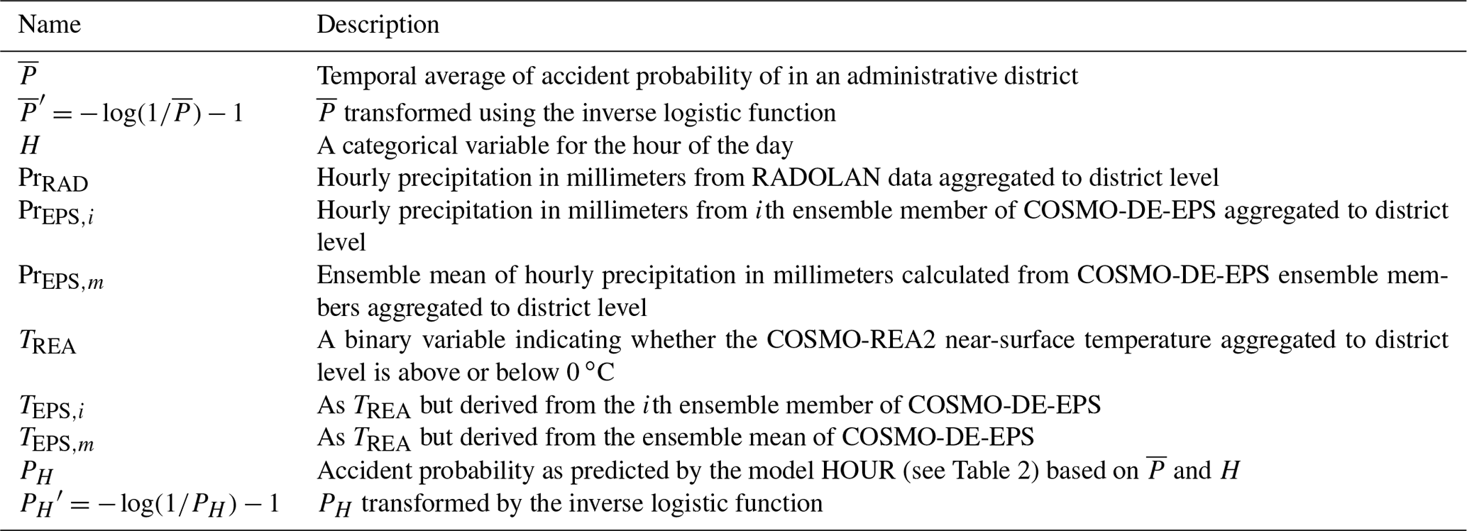
Table 2Description of different logistic regression models for hourly probabilities of weather-related road accidents in German administrative districts and their degrees of freedom (Df). Formulas are written using the statistical formula notation system as used in programming languages like R and Python, with colons indicating interaction terms. See Table 1 for a definition of variables.

The model HOUR includes an additional categorical variable H specifying the time of day in hours (local time), which describes the diurnal cycle additionally to the average accident probability of each district. These two models are used as reference models to assess the benefit of adding weather information.
3.4.2 Models using radar and reanalysis data
Accident, radar and reanalysis data overlap in time for the years from 2007 to 2012. For this time period, a binary predictor variable with hourly resolution for the near-surface temperature TREA (temperature at 2 m height) is derived from COSMO-REA2, which distinguishes between temperatures above and below 0 ∘C. Furthermore, a continuous variable PrRAD with the hourly precipitation sum in millimeters per hour is used. In the model RAD the model HOUR is extended by adding TREA and (PrRAD)0.2 as direct effects. Different combinations of exponents have been tested to transform the precipitation, but 0.2 leads to the best results in terms of model skill. In the model RAD_INT the two-point interaction terms between , H, TREA and (PrRAD)0.2 are added to the model equation. Model parameter estimates result from using data from all districts simultaneously. However, the skill scores are calculated for each district individually within the cross-validation procedure. This allows us to compare the performance of the model in different districts.
Additionally, we fit the models to the individual districts, yielding models RAD_IND and RAD_INT_IND1, respectively. On the one hand, these models capture the district-specific characteristics; on the other hand, the number of available data points for each model is strongly reduced, which complicates the estimation of model parameters, in particular for districts with low accident numbers. These models are used to quantify the benefit of having one model for all districts.
3.4.3 Models using weather forecast data
The overlapping time period of accident data and COSMO-DE-EPS data are the years 2011 and 2012. For this time period temperature and precipitation are aggregated to the district level as before for all 20 ensemble members. This is done separately for all forecast lead times τ, ranging between 1 h after forecast initialization and 21 h after initialization.
The COSMO-DE-EPS provides hourly forecast data but is initialized only every 3 h. Therefore, not all hours are available for all lead times. For example, a lead time of 6 h is only available at 00:00, 03:00, 06:00, 09:00, 12:00, 15:00, 18:00 and 21:00 UTC, while a lead time of 7 h is only available at 01:00, 04:00, 07:00, 10:00, 13:00, 16:00, 19:00 and 22:00 UTC. Furthermore, the logistic regression model uses local time, which has to take into account daylight savings time. Both effects complicate an explicit use of the hour as a predictor variable in combination with COSMO-DE-EPS data. Therefore, to facilitate the incorporation of a diurnal cycle in the model, a two-step procedure is applied. First, the model HOUR is used to forecast the average diurnal cycle of accident probabilities PH for each district. Second, PH is transformed into using the inverse logistic function. Then, is used to replace the terms (compare HOUR and EPS_HOUR in Table 2, for example).
Three different ways to incorporate the ensemble information in the models are used.
-
Deterministic forecasts: in the case of the model EPS_MEMi_INT, an individual set of parameters is estimated for each ensemble member and each lead time. Skill scores are calculated for each of the resulting sets of parameters separately, thus treating the ensemble members as single deterministic forecasts.
-
Meteorology-averaged ensemble: in the case of the model EPS_MEAN_INT, the parameters are estimated using the ensemble mean of the meteorological variables, which results in a single set of parameters for each lead time.
-
Probability-averaged ensemble: in the case of the model EPS_PMEAN_INT, accident probabilities are predicted using the models EPS_MEMi_INT for the individual ensemble members, but the ensemble mean of the predicted probabilities is calculated before using it to compute the scores in the cross-validation procedure.
The models EPS_HOUR and EPS_RAD_INT correspond to the models HOUR and RAD_INT but are fitted separately to the data available for each lead time to allow a direct comparison to the models using COSMO-DE-EPS data.
4.1 Models using radar and reanalysis data
The time-averaged hourly probability that at least one weather-related accident occurs in an administrative district is referred to as . It ranges from less than 0.001 for smaller districts with few inhabitants to more than 0.05 for densely populated cities. The NULL model simply gives for each district and serves as a reference model. As expected, the AUC is 0.5, indicating that the model is not able to distinguish between accident and nonaccident cases (Table 3).
Table 3Verification measures for models using radar and reanalysis data. Akaike information criterion (AIC), area under receiver operating characteristic curve (AUC), true positive rate (TPR), logarithmic score (LS) and Brier score (BS). Scores computed in a yearly cross-validation approach for each administrative district are shown as an average of all districts. Skill scores of AUC, LS and BS are computed with the model HOUR as reference (see Table 2). The best value of each score is written in bold.

In the model HOUR all parameters of the categorical variables H are significantly different from 0, with p values below 0.001, indicating that the diurnal cycle is an important aspect of the accident characteristics. The average AUC of all districts is 0.62, indicating that the introduction of the hour as a predictor improves the model.
The introduction of temperature and precipitation as direct effects in the model RAD leads to a further improvement of the scores compared to NULL and HOUR. With an AUC of about 0.81 and an AUCSS of 0.49 (HOUR as reference), temperature and precipitation can be considered useful in terms of binary classification of accident events. The TPR increases from 0.3 for HOUR to 0.7 for RAD. The interaction terms in RAD_INT slightly improve all scores except for the TPR.
Figure 1 shows that the variability of the AUCSS values of the different districts is relatively large compared to the differences between the models. However, there is no evident systematic relationship between the skill of the model and the geographic location of the district or the district-specific topography (not shown).

Figure 1Distribution of the cross-validated area under receiver operating characteristic curve skill score (AUCSS) of 401 administrative districts is shown for different logistic regression models for weather-related accident probabilities. The probability density is smoothed by a kernel density estimator (shading). The median is indicated by vertical dashed lines.
Figure 2 shows the modeled accident probabilities (solid lines) predicted by the RAD (panels a, c, e) and RAD_INT (panels b, d, f) versus precipitation (panels a and b), hour (panels c and d) and (panels e and f) together with the 95 % confidence intervals estimated from the standard errors (shaded). Additionally, the accident probabilities estimated nonparametrically (number of time steps with accidents divided by total number of time steps) are shown (markers) together with the 95 % confidence intervals estimated using a bootstrapping approach (vertical lines). Model and nonparametric probabilities are shown for positive (red) and negative (blue) temperatures.
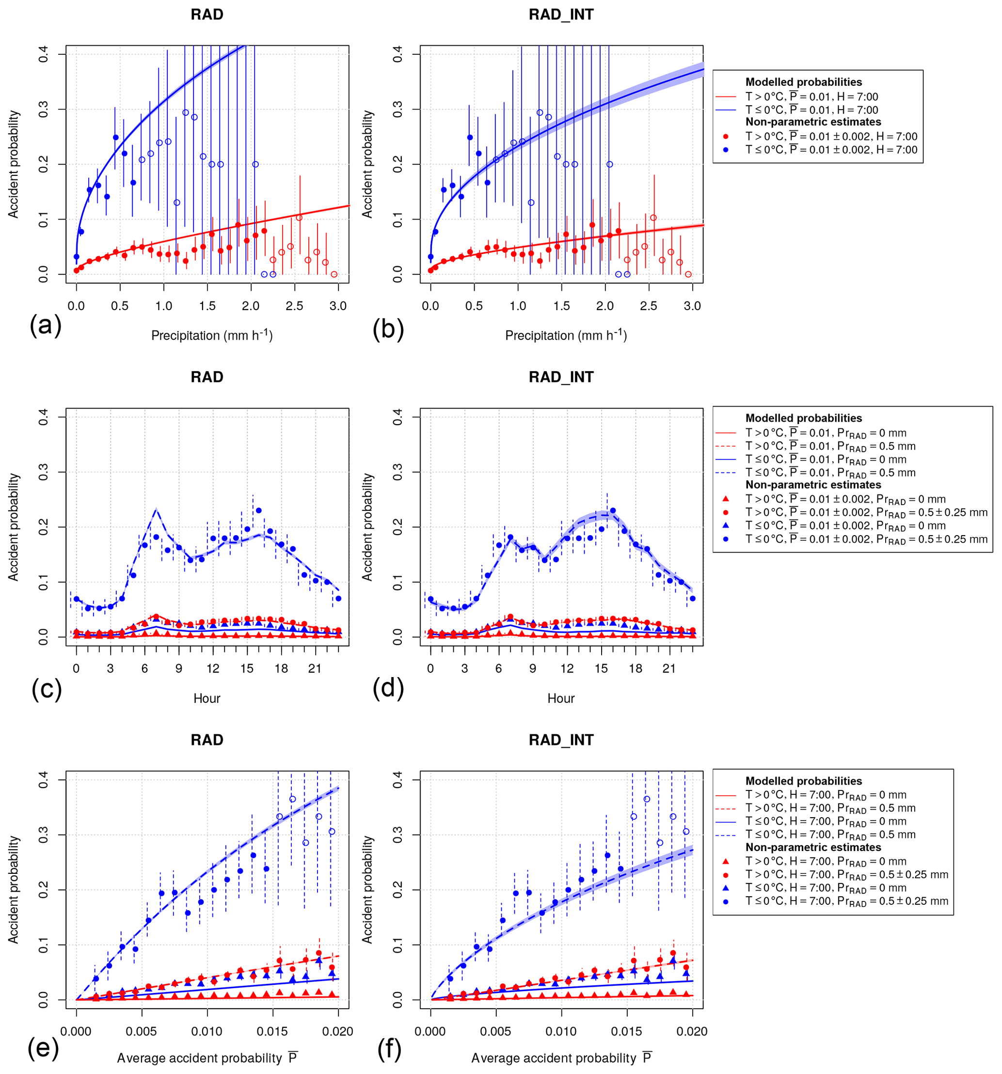
Figure 2Comparison of modeled probabilities of weather-related road accidents with nonparametric probability estimates. Probabilities (lines) and 95 % confidence intervals based on standard errors (shading) of the model RAD (a, c, e) and RAD_INT (b, d, f) are displayed as a function of hourly precipitation (a, b), hour of the day (c, d) and the temporal average accident probability of the administrative district (e, f) for different parameter settings (see legends for details). Nonparametric estimates of probabilities (markers) and 95 % confidence intervals based on bootstrapping (vertical lines) are shown for corresponding parameter ranges.
The modeled accident probabilities as a function of PrRAD are shown for 07:00 local time for a district with an average probability for weather-related accidents of (Fig. 2a and b). Nonparametric probability estimates are calculated for precipitation bins with a width of 0.1 mm h−1 including only districts with . In general, accident probabilities are lowest at PrRAD=0 and show a steep increase with increasing precipitation and a decreasing slope at higher precipitation rates. Probabilities are higher at temperatures below 0 ∘C. At PrRAD=1 mm h−1, probabilities are about 5 times higher if temperatures are below 0 ∘C. For RAD the modeled probabilities fit well to the nonparametric probability estimates at PrRAD<0.5 mm h−1 but overestimate probabilities at higher precipitation rates. In contrast, the model RAD_INT shows reduced probabilities, which fit much better to the nonparametric probability estimates. The curved shape of the functional relationship between precipitation and probability is realized by taking precipitation to the power of 0.2. The value 0.2 was found to be the best choice after testing a series of different exponents; other functional relationships, for example log (1+Pr); and categories of precipitation.
The modeled probabilities as a function of H are shown for PrRAD=0 mm h−1 (solid lines) and PrRAD=0.5 mm h−1 (dashed lines) for (Fig. 2c and d). Nonparametric probability estimates are calculated using time steps with PrRAD=0 mm h−1 (circles) and mm h−1 (triangles) including only districts with . In general, accident probabilities show a pronounced diurnal cycle with maximum probabilities during morning and afternoon rush hours. RAD overestimates the observed probabilities in particular during the morning hours with precipitation at negative temperatures. The model RAD_INT is able to capture the observed diurnal cycle more precisely.
The modeled probabilities as function of are shown for PrRAD=0 mm h−1 (solid lines) and PrRAD=0.5 mm h−1 (dashed lines) at H=7 h (Fig. 2e and f). Nonparametric probability estimates are calculated using time steps with PrRAD=0 mm h−1 (circles) and mm h−1 (triangles) including districts with . In general, the probabilities show a monotonic increase with , which justifies the introduction of as a predictor to distinguish between different districts. The predictions of RAD and RAD_INT are relatively similar and lie mostly within the confidence intervals of the observed probabilities.
For more detailed insight into the modeling results, we provide the full model coefficients, standard errors and p values of the models NULL, HOUR, RAD and RAD_INT in the Supplement. In the case of RAD, which has 27 coefficients, almost all model coefficients have p values below 0.001, and we can reject the null hypothesis that the coefficients are 0. Only 1 of the 23 coefficients of the categorical variable HOUR is not significant. In the case of RAD_INT, which has 99 coefficients due to the introduction of interaction terms, 34 coefficients have p values below 0.001; 29 have p values greater than 0.1 and are thus not significantly different from 0. These nonsignificant coefficients all belong to the categorical variable HOUR or are included in an interaction term with this variable. This might indicate that the diurnal cycle could be modeled sufficiently with fewer than the 23 coefficients used here. However, we do not expect a large impact of such a reduction on the metrics that have been discussed earlier.
Next, we compare the models RAD and RAD_INT, which are fitted to all districts simultaneously, to the models RAD_IND and RAD_INT_IND, which are fitted to all districts individually. Figure 3 shows the difference of the AUCSS between RAD and RAD_IND (red) and between RAD_INT and RAD_INT_IND (black) as a function of . provides direct information about how many accident cases were available in the time series used for training the models. In general, the AUCSS differences are mostly negative, indicating that the models fitted to each district individually perform poorer than the models including all districts. The AUCSS differences decrease with increasing , i.e., increasing accident numbers. Furthermore, the AUCSS differences are larger for the more complex models with interaction terms. The results are similar for the LSS (not shown).
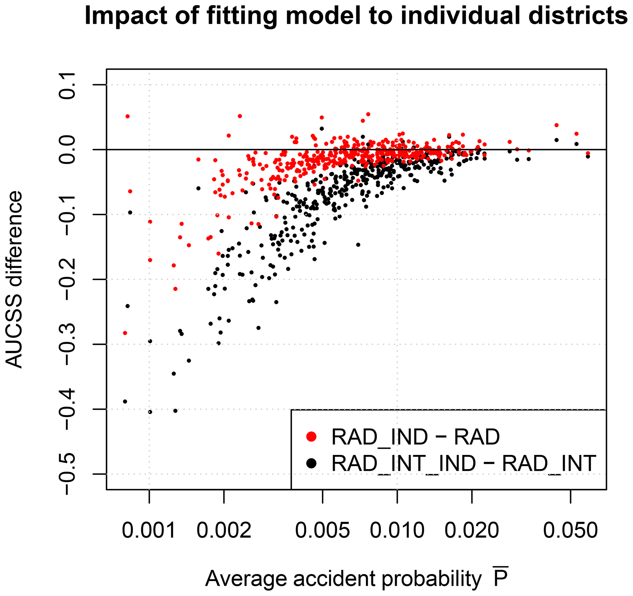
Figure 3Differences in area under receiver operating characteristic curve skill score (AUCSS) values between the models RAD_IND and RAD (red) and RAD_INT_IND and RAD_INT (black). AUCSS differences are shown for each of the 401 administrative districts vs. the average accident probability of the respective districts (dots).
Based on the results of this section, we can conclude that RAD_INT should be preferred over RAD since it achieves the best scores and better represents the functional relationship between probability and precipitation as well as the diurnal cycle. Furthermore, RAD_INT preforms better than RAD_INT_IND, which is fitted to each district individually.
4.2 Models using weather forecast data
The model RAD_INT showed the best performance among the models predicting accident probability using radar and reanalysis data (Sect. 4.1). In this section the model formulation of RAD_INT is modified to allow the use of COSMO-DE-EPS ensemble weather forecasts. To facilitate the modeling procedure, the variables H and are combined into a single variable by using the model HOUR, which effectively results in a district-specific diurnal cycle of accident probabilities (see Sect. 3.4.3 for details). , precipitation and temperature are used as predictor variables, including their interaction terms. For each lead time from 1 to 21 h, a new set of model parameters is estimated using only those time steps where COSMO-DE-EPS data are available for the specific lead time. For a small number of forecasts the COSMO-DE-EPS data are missing or incomplete.
The model EPS_RAD_INT uses TREA and PrRAD and serves as a reference, representing the best available model based on reanalysis and radar data. The AUCSS of EPS_RAD_INT as a function of lead time shows a 3-hourly cyclic pattern with maximum values of around 0.5 at lead times 1, 4, 7, etc. and 0.47 in between (Fig. 4, orange line). This cyclic pattern occurs because hourly data are used in the statistical models, but COSMO-DE-EPS is only initialized every 3 h (00:00, 03:00, 06:00 UTC, etc.). Consequently, EPS_RAD_INT for lead times of 1, 4, 7 h, etc. includes only data at 01:00, 04:00, 07:00 UTC, etc.; the lead times 2, 5, 8 h, etc. include only 02:00, 05:00, 08:00 UTC, etc.; and the lead times 3, 6, 9 h, etc. include only 00:00, 03:00, 06:00 UTC, etc. As a consequence, there are three sets of lead times that are associated with different sets of hours of the day, which correspond to the repetitive 3-hourly pattern in the AUCSS. Apparently, the model performs differently for these three sets of hours, possibly due to different traffic characteristics during the specific hours.

Figure 4Area under receiver operating characteristic curve skill score (AUCSS) values of different models for hourly probabilities of weather-related road accidents using radar, reanalysis and weather forecast data from 2011 to 2012 as a function of lead time.
The model EPS_MEMi_INT is estimated for each of the 20 ensemble members individually, which therefore results in 20 deterministic forecasts with 20 individual AUCSS values per lead time. The AUCSS drops from 0.48 at lead time 1 h to below 0.45 at lead time 21 h (gray lines). The spread between the AUCSS of the different ensemble members increases with increasing lead time. The model EPS_MEAN_INT is based on the ensemble mean of the meteorological variables (meteorology-averaged ensemble) and shows a slightly higher AUCSS (solid black line) than all the deterministic forecasts.
The model EPS_PMEAN_INT, which is based on the ensemble mean of the accident probabilities of the 20 versions of EPS_MEMi_INT (probability-averaged ensemble), shows again a slightly higher AUCSS (dashed black line) than the meteorology-averaged ensemble. As expected, the AUCSS values of all models based on weather forecast data are lower than the AUCSS of EPS_RAD_INT based on radar and reanalysis data. However, the differences are relatively small. The LSS shows a similar behavior regarding the lead time dependence as the AUCSS (not shown).
4.3 Case study
The models RAD_INT and EPS_PMEAN_INT are used in a case study with adverse winter weather conditions on 3 December 2012. At temperatures below the freezing point the fronts of a low-pressure system lead to snowfall in large parts of Germany. These weather conditions lead to a total number of 280 accidents classified by the police as caused by road condition. The majority of the accidents occurred in southern and western Germany.2
For the district of Stuttgart, which was located within the affected area, the RADOLAN data show low precipitation amounts in the early morning and higher precipitation amounts of up to 0.3 mm h−1 in the afternoon (Fig. 5a). The COSMO-DE-EPS forecast, which was initialized on 3 December 2012 at 00:00 UTC (02:00 LT, local time), shows ensemble mean precipitation amounts of more than 0.6 mm h−1 in the afternoon and a large spread between the ensemble members.
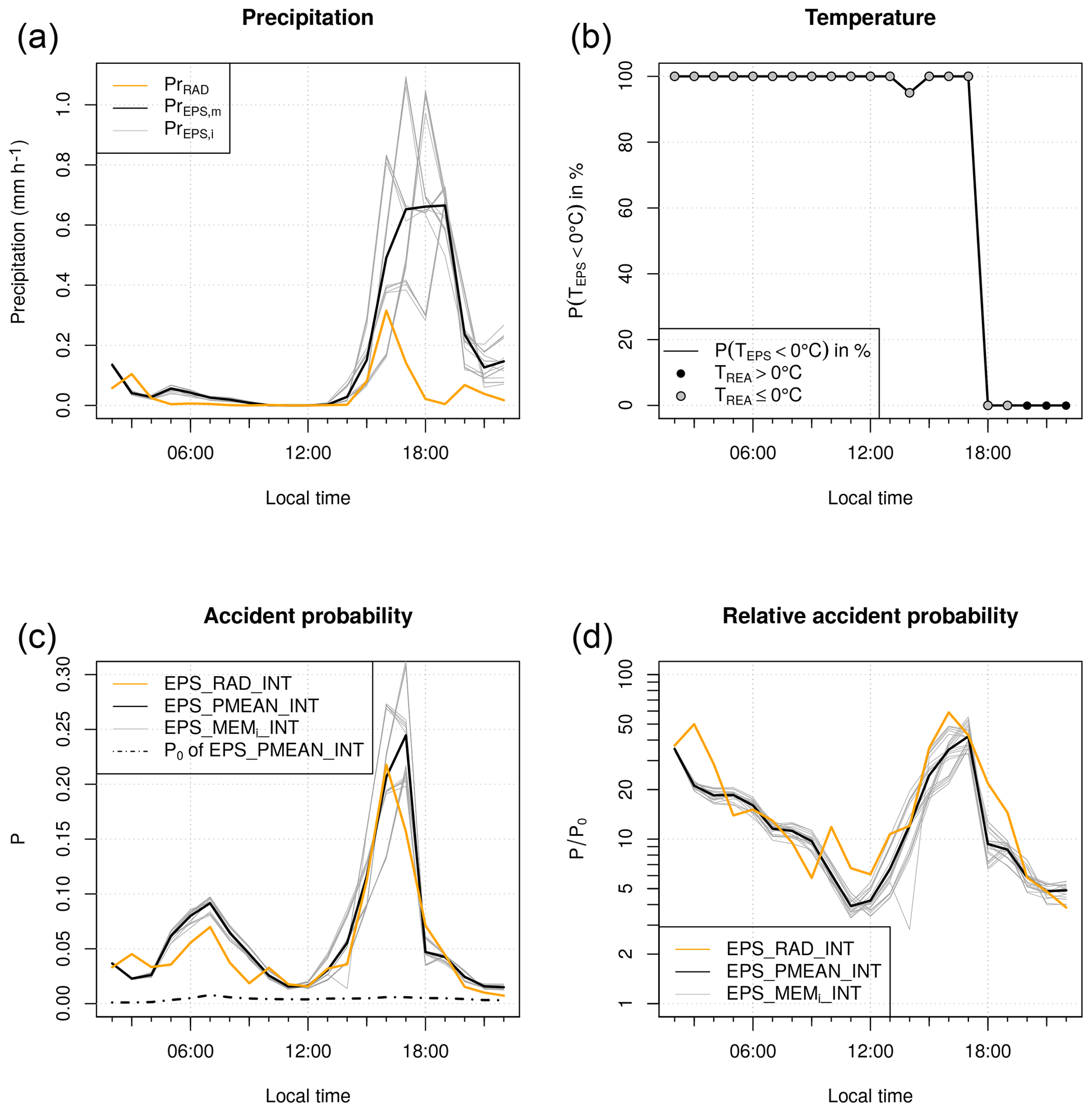
Figure 5Application of the models EPS_RAD_INT and EPS_PMEAN_INT to an adverse winter weather event on 3 December 2012. Time series are shown for the district of Stuttgart using the COSMO-DE-EPS forecast initialized at 00:00 UTC. (a) Hourly precipitation aggregated to district level, (b) percentage of ensemble members with temperatures below 0 ∘C, (c) probability of weather-related road accidents and (d) relative accident probability.
The temperature in COSMO-REA2 is below 0 ∘C until 19:00 LT and then changes to warmer conditions (Fig. 5b). All ensemble members of COSMO-DE-EPS predict the change to positive temperatures 2 h earlier than observed.
The accident probability of EPS_RAD_INT shows the combined effect of the average diurnal cycle, RADOLAN precipitation and COSMO-REA2 temperature (Fig. 5c). It shows a peak of 0.07 in the morning during rush hour at low precipitation amounts at freezing temperatures; a drop to 0.02 at noon, when RADOLAN shows no precipitation; and a maximum peak of 0.22 in the afternoon, when precipitation is strongest. In general, the accident probability of EPS_PMEAN_INT matches well with EPS_RAD_INT. However, it slightly overestimates the morning peak and overestimates the afternoon peak due to the too intense and persistent precipitation.
The hourly accident probability P is useful for authorities to assess how likely the occurrence of an accident is in a certain district at a certain point in time. However, it does not reflect the risk of an individual road user as it does not distinguish whether P changes due to weather-related effects, due to a change in traffic density along the diurnal cycle or due to the district characteristics. For example, a road user traveling from a district with a high average accident probability to a district with a low would observe a decrease in P even if the weather conditions remain the same. Therefore, to estimate the impact on an individual road user, we compare P to P0, the probability under conditions without precipitation and with positive temperatures (Fig. 5c, dotted line). The fraction P∕P0 gives the amplification of the actual predicted probability P compared to warm and dry conditions (Fig. 5d). In the case of the forecast for 3 December 2012, the amplification factor ranges between 50 in the afternoon, when the precipitation amount is high, and 5 around noon, when the precipitation amount is low. This factor could be a potential weather impact forecast product.
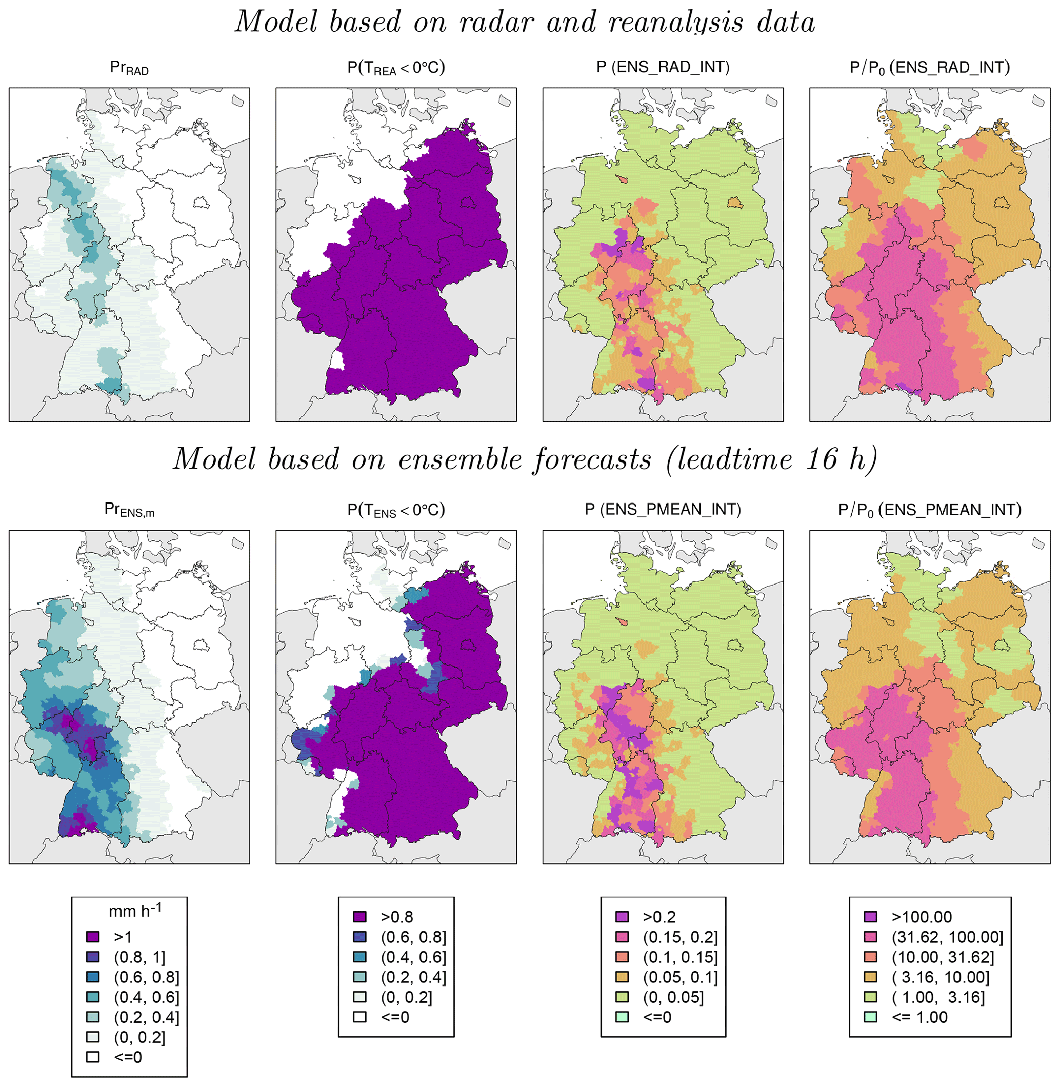
Figure 6Model results for adverse winter weather conditions on 3 December 2012 at 17:00 LT based on models EPS_RAD_INT (top) and EPS_PMEAN_INT using the COSMO-DE-EPS forecast with a lead time of 16 h initialized at 00:00 UTC (bottom). From left to right: hourly precipitation at district level, fraction of ensemble members with temperatures below 0 ∘C, probability of weather-related road accidents and relative accident probability.
On 3 December 2012 at 17:00 LT, the COSMO-DE-EPS overestimates the precipitation amount in large parts of western and southern Germany compared to RADOLAN (Fig. 6). The area with temperatures below 0 ∘C is captured relatively well compared to COSMO-REA2. The accident probability P is largest where high precipitation amounts and freezing temperatures occur. Spatially, P is relatively inhomogeneous, which reflects the large differences in average accident probability between the individual districts. P∕P0, representing the increase in accident probability of individual drivers, is spatially more homogeneous.
Police reports of heavy road accidents in Germany were used to construct hourly time series based on weather-related accidents caused by adverse road conditions for German administrative districts. Different meteorological data sets aggregated to the district level were used in logistic regression models to predict hourly accident probabilities. Models of different complexity were compared after calculating different skill scores using a yearly cross-validation approach. The best model with respect to these scores included district-specific average accident probability, the hour of the day, hourly precipitation and temperature, and their interaction terms. The model reached a hit rate (TPR) of 0.7 when the false-alarm rate (FPR) was fixed at 0.2. With the same false-alarm rate, a model without meteorological parameters only reached a hit rate of 0.3. It was shown that the probability of weather-related accidents increases nonlinearly with increasing hourly precipitation. Given an hourly precipitation of 1 mm, the accident probability is approximately 5 times higher at negative temperatures compared to positive temperatures. In a case study it was shown that the model is able to reasonably capture the spatial and temporal development of accident probabilities during adverse winter weather conditions. When using ensemble weather forecasts to predict accident probabilities, the skill of the logistic regression model remains almost constant for a forecast lead time of up to 21 h. Furthermore, the use of ensemble forecasts leads to a higher skill compared to a setting where ensemble members are treated as individual deterministic forecasts. These findings are in line with the results of Pardowitz et al. (2016), who show that the use of ensemble information improves predictions of storm damage probabilities.
The target variable of this study was weather-related road accidents. The accidents included in the analysis were indicated by the police as being caused by adverse road conditions, which includes a wet, snowy or icy road but also mud or dirt on the road. Thus, the categorization of the accident cause is based on the subjective decision of the police at the location of the accident. This might introduce a bias to the results whose direction or extent is hard to estimate. For example, a large number of accidents that occur during adverse weather conditions are likely to be unrelated to the weather but are caused only by inattention of the driver. Police officers might still categorize these accidents as being weather-related in unclear situations. It should be kept in mind that this could lead to an overestimation of weather-related accident probabilities in the models developed in this study.
It is known that the main parameters affecting accident probability are traffic flow and density. In an optimal case one would use measurements of these variables as a model predictor for accident probability. However, traffic measurements are not continuously available for all administrative districts. Additionally, measurements of traffic flow are mainly available for highways and federal roads and might not be representative for municipal roads, where the majority of the accidents occur. Furthermore, in an operational setting, where the model is applied for predicting future accident probabilities, traffic measurements are not available. Therefore, we decided not to directly include traffic measurements in the models. Instead, the hour of the day was used as a categorical predictor variable to capture the average diurnal cycle of accident probability. It was shown that this approach is able to reasonably represent the inner-day variability of accident probability. The introduction of additional factors like on weekends or holidays did not lead to a significant improvement of the model.
It is a challenging task to combine accident data, which are available for the area of administrative districts, with meteorological data, which are usually available in the form of point observations or gridded data. Different ways of aggregating meteorological data to the district level were tested, and the approach based on distance-weighted averaging, which is presented in this study, showed the best results.
The temperature at 2 m height was used in this study to include the effect of negative temperatures in the statistical model in a relatively simple approach. It has the benefit that the temperature at 2 m height is a well-established meteorological parameter, which is measured at most stations and available in all weather forecasting models. However, it might not reflect the conditions at the road surface, which can deviate from the conditions at 2 m height. Also, the choice of 0 ∘C as a fixed threshold is a simplified approach since ground frost or snowfall could also occur at higher 2 m temperatures. By using nonlinear approaches like generalized additive models (Wood, 2017) a smooth transition between positive and negative temperatures could be established in future studies. Furthermore, it might be detrimental that area averaged temperatures are used, which does not fully represent topographic variations within the area of a certain district. A more complex approach could make use of a road surface model, which includes the combined effects of precipitation, evaporation, and road surface temperatures in a more sophisticated way (e.g., Juga et al., 2013).
In addition to the weather parameters presented in this study, other parameters like snow fall amount or combined measures of cloud cover and sun angle to describe the impact of sun glare were tested as potential predictor variables. Furthermore, advanced predictor selection techniques like genetic algorithms (Calcagno and de Mazancourt, 2010) and the least absolute shrinkage and selection operator (Tibshirani, 1996) were applied to find optimal combinations of parameters. However, none of the results were able to significantly improve the skill of the best models presented in this study, as measured by the cross-validation approach.
We found that the probability of weather-related accidents depends on hourly precipitation to the power of 0.2. This exponent should not be understood as a universal relationship. Instead, it is likely to depend on different aspects of the road system (e.g., how fast the water is able to leave the road surface) or the average car characteristics (e.g., the share of cars equipped with assistance systems or the type of tires). It may even change in time as road and car qualities improve.
In this work we showed two ways of modeling probabilities in different districts: first, by creating a model that distinguishes between different districts based on their average accident probability and, second, by creating a model for each district individually. We found that the first approach leads to higher skill scores, particularly for districts with low accident numbers. Including additional district-specific parameters describing the characteristics of the road network or topographic conditions could help to further refine the model.
This study shows that a skillful relationship between meteorological parameters and weather-related road accidents can be established. Forecasts of probabilities of weather-related road accidents, as presented in this study, might be useful for authorities (traffic management, police or emergency services) on the one hand and road users on the other hand. However, it is reasonable to provide the information about accident risk in different, user-specific formats, which are introduced in Sect. 4.3. Authorities might be primarily interested in aggregated risk information for their region of interest, e.g., the occurrence probability of accidents in an administrative district. On the other hand, road users are rather interested in their individual risk. The individual risk is better reflected through an amplification of risk compared to certain reference conditions (e.g., warm and dry weather).
It was shown that impact-based warning can lead to better actions of the recipients (Weyrich et al., 2018). Furthermore, Hemingway and Robbins (2019) state that information about weather impacts can be helpful for operational meteorologists when issuing weather warnings. This was found using a prototype impact model for predicting the risk of road disruption due to the wind-induced overturning of vehicles. In this context, the accident model presented in this study can be considered a useful tool for reduction in road traffic risk.
The accident data for Germany were obtained from the Research Data Centre of the Federal Statistical Office and Statistical Offices of the Länder. The RADOLAN data set (Bartels et al., 2004) is available at https://www.dwd.de/DE/leistungen/radolan/radolan.html (last access: 28 October 2020). The COSMO-REA2 data set (Wahl et al., 2017) is available at https://reanalysis.meteo.uni-bonn.de/?Download_Data___COSMO-REA2 (last access: 28 October 2020). The COSMO-DE-EPS data were provided by the Deutscher Wetterdienst upon request.
The supplement related to this article is available online at: https://doi.org/10.5194/nhess-20-2857-2020-supplement.
Data analysis and visualization were done by NB; all authors contributed to writing the manuscript.
The authors declare that they have no conflict of interest.
This research was carried out within the framework of the Hans-Ertel-Centre for Weather Research. This research network of universities, research institutes and the Deutscher Wetterdienst is funded by the Bundesministerium für Verkehr und Digitale Infrastruktur.
This research has been supported by the Bundesministerium für Verkehr und Digitale Infrastruktur (grant no. 4818DWDP3A).
We acknowledge support from the Open Access Publication
Initiative of Freie Universität Berlin.
This paper was edited by Joaquim G. Pinto and reviewed by three anonymous referees.
Ahmed, M. M., Abdel-Aty, M., and Yu, R.: Assessment of interaction of crash occurrence, mountainous freeway geometry, real-time weather, and traffic data, Transp. Res. Record, 2280, 51–59, https://doi.org/10.3141/2280-06, 2012. a
Akaike, H.: A new look at the statistical model identification, IEEE Trans. Automat. Contr., 19, 716–723, https://doi.org/10.1007/978-1-4612-1694-0_16, 1974. a
Bartels, H., Weigl, E., Reich, T., Lang, P., Wagner, A., Kohler, O., and Gerlach, N.: Projekt RADOLAN – Routineverfahren zur Online-Aneichung der Radarniederschlagsdaten mit Hilfe von automatischen Bodenniederschlagsstationen (Ombrometer), Deutscher Wetterdienst, Hydrometeorologie, available at: https://www.dwd.de/DE/leistungen/radolan/radolan.html (last access: 28 October 2020), 2004. a, b
BASt: Verkehrs- und Unfalldaten – Kurzzusammenstellung der Entwicklung in Deutschland, Tech. rep., Bundesanstalt für Straßenwesen, Bergisch Gladbach, Germany, 2017. a
Benedetti, R.: Scoring rules for forecast verification, Mon. Weather Rev., 138, 203–211, https://doi.org/10.1175/2009MWR2945.1, 2010. a
Bergel-Hayat, R. and Depireb, A.: Climate, Road Traffic and Road Risk: An Aggregate Approach, in: 10th World Conference on Transport Research, availab 28 October 2020), 2004. a, b
Brier, G. W.: Verification of forecasts expressed in terms of probability, Mon. Weather Rev., 78, 1–3, https://doi.org/10.1175/1520-0493(1950)078<0001:VOFEIT>2.0.CO;2, 1950. a
Brijs, T., Karlis, D., and Wets, G.: Studying the effect of weather conditions on daily crash counts using a discrete time-series model, Accident Anal. Prev., 40, 1180–1190, https://doi.org/10.1016/j.aap.2008.01.001, 2008. a, b
Brodsky, H. and Hakkert, A. S.: Risk of a road accident in rainy weather, Accident Anal. Prev., 20, 161–176, https://doi.org/10.1016/0001-4575(88)90001-2, 1988. a
Calcagno, V. and de Mazancourt, C.: glmulti: an R package for easy automated model selection with (generalized) linear models, J. Stat. Softw., 34, 1–29, https://doi.org/10.18637/jss.v034.i12, 2010. a
Caliendo, C., Guida, M., and Parisi, A.: A crash-prediction model for multilane roads, Accident Anal. Prev., 39, 657–670, https://doi.org/10.1016/j.aap.2006.10.012, 2007. a, b
Cho, J., Lee, H., and Yoo, W.: A wet-road braking distance estimate utilizing the hydroplaning analysis of patterned tire, Int. J. Numer. Meth. Eng., 69, 1423–1445, https://doi.org/10.1002/nme.1813, 2007. a
Dobson, A. J. and Barnett, A. G.: An introduction to generalized linear models, Chapman and Hall/CRC, Boca Raton, United States, 2008. a
Eisenberg, D.: The mixed effects of precipitation on traffic crashes, Accident Anal. Prev., 36, 637–647, https://doi.org/10.1016/S0001-4575(03)00085-X, 2004. a, b, c
Fridstrøm, L. and Ingebrigtsen, S.: An aggregate accident model based on pooled, regional time-series data, Accident Anal. Prev., 23, 363–378, https://doi.org/10.1016/0001-4575(91)90057-C, 1991. a
Fridstrøm, L., Ifver, J., Ingebrigtsen, S., Kulmala, R., and Thomsen, L. K.: Measuring the contribution of randomness, exposure, weather, and daylight to the variation in road accident counts, Accident Anal. Prev., 27, 1–20, https://doi.org/10.1016/0001-4575(94)E0023-E, 1995. a, b, c
Gebhardt, C., Theis, S., Paulat, M., and Bouallègue, Z. B.: Uncertainties in COSMO-DE precipitation forecasts introduced by model perturbations and variation of lateral boundaries, Atmos. Res., 100, 168–177, https://doi.org/10.1016/j.atmosres.2010.12.008, 2011. a
Hanley, J. A. and McNeil, B. J.: The meaning and use of the area under a receiver operating characteristic (ROC) curve, Radiology, 143, 29–36, https://doi.org/10.1148/radiology.143.1.7063747, 1982. a
Hays, D. and Browne, A. L.: The physics of tire traction: theory and experiment, Springer Science & Business Media, New York, United States, 1974. a
Hemingway, R. and Robbins, J.: Developing a hazard impact model to support impact-based forecasts and warnings: The Vehicle OverTurning Model, Meteorol. Appl., 27, e1819, https://doi.org/10.1002/met.1819, 2019. a
Hermans, E., Brijs, T., Stiers, T., and Offermans, C.: The impact of weather conditions on road safety investigated on an hourly basis, in: TRB 85th Annual Meeting Compendium of Papers, 1–16, Transportation Research Board, available at: http://hdl.handle.net/1942/1365 (last access: 28 October 2020), 2006a. a, b, c
Hermans, E., Wets, G., and Van den Bossche, F.: Frequency and severity of Belgian road traffic accidents studied by state-space methods, J. Transp. Stat., 9, 63–76, 2006b. a
Jaroszweski, D. and McNamara, T.: The influence of rainfall on road accidents in urban areas: A weather radar approach, Travel. Behav. Soc., 1, 15–21, https://doi.org/10.1016/j.tbs.2013.10.005, 2014. a
Juga, I., Nurmi, P., and Hippi, M.: Statistical modelling of wintertime road surface friction, Meteorol. Appl., 20, 318–329, https://doi.org/10.1002/met.1285, 2013. a
Keay, K. and Simmonds, I.: The association of rainfall and other weather variables with road traffic volume in Melbourne, Australia, Accident Anal. Prev., 37, 109–124, https://doi.org/10.1016/j.aap.2004.07.005, 2005. a
Keay, K. and Simmonds, I.: Road accidents and rainfall in a large Australian city, Accident Anal. Prev., 38, 445–454, https://doi.org/10.1016/j.aap.2005.06.025, 2006. a
Knapp, K. K., Smithson, L. D., and Khattak, A. J.: Mobility and safety impacts of winter storm events in a freeway environment, Tech. rep., Center for Transportation Research and Education, Iowa State University, available at: https://rosap.ntl.bts.gov/view/dot/23579 (last access: 28 October 2020), 2000. a, b
Malin, F., Norros, I., and Innamaa, S.: Accident risk of road and weather conditions on different road types, Accident Anal. Prev., 122, 181–188, https://doi.org/10.1016/j.aap.2018.10.014, 2019. a
Martin, J.-L.: Relationship between crash rate and hourly traffic flow on interurban motorways, Accident Anal. Prev., 34, 619–629, https://doi.org/10.1016/S0001-4575(01)00061-6, 2002. a
Menard, S.: Applied logistic regression analysis, Vol. 106 of Quantitative Applications in the Social Sciences, SAGE Publications, Thousand Oaks, United States, 2002. a
Mills, B., Andrey, J., Doberstein, B., Doherty, S., and Yessis, J.: Changing patterns of motor vehicle collision risk during winter storms: A new look at a pervasive problem, Accident Anal. Prev., 127, 186–197, https://doi.org/10.1016/j.aap.2019.02.027, 2019. a, b
Pardowitz, T., Osinski, R., Kruschke, T., and Ulbrich, U.: An analysis of uncertainties and skill in forecasts of winter storm losses, Nat. Hazards Earth Syst. Sci., 16, 2391–2402, https://doi.org/10.5194/nhess-16-2391-2016, 2016. a
Peden, M., Scurfield, R., Sleet, D., Mohan, D., Hyder, A. A., Jarawan, E., and Mathers, C. D.: World report on road traffic injury prevention, 2004. a
Peralta, C., Ben Bouallègue, Z., Theis, S., Gebhardt, C., and Buchhold, M.: Accounting for initial condition uncertainties in COSMO-DE-EPS, J. Geophys. Res.-Atmos., 117, D07108, https://doi.org/10.1029/2011JD016581, 2012. a
Scott, P.: Modelling time-series of British road accident data, Accident Anal. Prev., 18, 109–117, https://doi.org/10.1016/0001-4575(86)90055-2, 1986. a, b
Shankar, V., Mannering, F., and Barfield, W.: Effect of roadway geometrics and environmental factors on rural freeway accident frequencies, Accident Anal. Prev., 27, 371–389, https://doi.org/10.1016/0001-4575(94)00078-Z, 1995. a, b
Shmueli, G.: To explain or to predict?, Stat. Sci., 25, 289–310, https://doi.org/10.1214/10-STS330, 2010. a
Stephan, K., Klink, S., and Schraff, C.: Assimilation of radar-derived rain rates into the convective-scale model COSMO-DE at DWD, Q. J. Roy. Meteor. Soc., 134, 1315–1326, https://doi.org/10.1002/qj.269, 2008. a
Stipdonk, H. and Berends, E.: Distinguishing traffic modes in analysing road safety development, Accident Anal. Prev., 40, 1383–1393, https://doi.org/10.1016/j.aap.2008.03.001, 2008. a
Theofilatos, A. and Yannis, G.: A review of the effect of traffic and weather characteristics on road safety, Accident Anal. Prev., 72, 244–256, https://doi.org/10.1016/j.aap.2014.06.017, 2014. a
Tibshirani, R.: Regression shrinkage and selection via the lasso, J. R. Stat. Soc., 58, 267–288, https://doi.org/10.1111/j.2517-6161.1996.tb02080.x, 1996. a
Tiedtke, M.: A comprehensive mass flux scheme for cumulus parameterization in large-scale models, Mon. Weather Rev., 117, 1779–1800, https://doi.org/10.1175/1520-0493(1989)117<1779:ACMFSF>2.0.CO;2, 1989. a
Wahl, S., Bollmeyer, C., Crewell, S., Figura, C., Friederichs, P., Hense, A., Keller, J. D., and Ohlwein, C.: A novel convective-scale regional reanalyses COSMO-REA2: Improving the representation of precipitation, Meteorol. Z., 26, 345–361, https://doi.org/10.1127/metz/2017/0824, 2017 (data available at: https://reanalysis.meteo.uni-bonn.de/?Download_Data___COSMO-REA2, last access: 28 October 2020). a, b, c
Weyrich, P., Scolobig, A., Bresch, D. N., and Patt, A.: Effects of impact-based warnings and behavioral recommendations for extreme weather events, Weather Clim. Soc., 10, 781–796, https://doi.org/10.1175/WCAS-D-18-0038.1, 2018. a
Wood, S. N.: Generalized additive models: an introduction with R, Chapman and Hall/CRC, Boca Raton, United States, 2017. a, b
Yannis, G. and Karlaftis, M. G.: Weather effects on daily traffic accidents and fatalities: a time series count data approach, in: Proceedings of the 89th Annual Meeting of the Transportation Research Board, The National Academies of Sciences, Engineering, and Medicine, Washington, United States, 10–14, 2010. a
Ziakopoulos, A. and Yannis, G.: A review of spatial approaches in road safety, Accident Anal. Prev., 135, 105323, https://doi.org/10.1016/j.aap.2019.105323, 2020. a
INT refers to the use of interaction terms in the model equation, while IND refers to estimating model parameters for each district individually.
Due to regulations regarding anonymization and data protection we are not allowed to show accident counts less than three, which prevents us from showing accident counts for single hours or days at the district level.