the Creative Commons Attribution 4.0 License.
the Creative Commons Attribution 4.0 License.
Simulation of extreme rainfall and streamflow events in small Mediterranean watersheds with a one-way-coupled atmospheric–hydrologic modelling system
Adriana Bruggeman
George Zittis
Ioannis Sofokleous
Joël Arnault
Coupled atmospheric–hydrologic systems are increasingly used as instruments for flood forecasting and water management purposes, making the performance of the hydrologic routines a key indicator of the model functionality. This study's objectives were (i) to calibrate the one-way-coupled WRF-Hydro model for simulating extreme events in Cyprus with observed precipitation and (ii) to evaluate the model performance when forced with WRF-downscaled (1×1 km2) re-analysis precipitation data (ERA-Interim). This set-up resembles a realistic modelling chain for forecasting applications and climate projections. Streamflow was modelled during extreme rainfall events that occurred in January 1989 (calibration) and November 1994 (validation) over 22 mountain watersheds. In six watersheds, Nash–Sutcliffe efficiencies (NSEs) larger than 0.5 were obtained for both events. The WRF-modelled rainfall showed an average NSE of 0.83 for January 1989 and 0.49 for November 1994. Nevertheless, hydrologic simulations of the two events with the WRF-modelled rainfall and the calibrated WRF-Hydro returned negative streamflow NSE for 13 watersheds in January 1989 and for 18 watersheds in November 1994. These results indicate that small differences in amounts or shifts in time or space of modelled rainfall, in comparison with observed precipitation, can strongly modify the hydrologic response of small watersheds to extreme events. Thus, the calibration of WRF-Hydro for small watersheds depends on the availability of observed rainfall with high temporal and spatial resolution. However, the use of modelled precipitation input data will remain important for studying the effect of future extremes on flooding and water resources.
- Article
(5843 KB) - Full-text XML
-
Supplement
(2819 KB) - BibTeX
- EndNote
Atmospheric and hydrologic processes are strictly related, since they share the land surface as a common interface for moisture and heat fluxes. Precipitation is the primary cause of all surface hydrologic processes, such as overland, subsurface and river flow. Conversely, soil moisture and surface water distributions affect near-surface atmospheric conditions and processes, such as the temperature distribution, the structure of the atmospheric boundary layer, the formation of shallow clouds and precipitation amounts (Lin and Cheng, 2016; Zittis et al., 2014, and references therein). In recent years, the scientific community has made ever-increasing efforts to improve the simulation skills of both atmospheric and hydrologic models, leading also to the development of coupled modelling systems. Since the beginning of the 21st century, the main research interest in developing such models has been the evaluation of the feedbacks between the hydrologic cycle and the atmospheric processes, to get a deeper understanding of regional climate change and its impacts (Ning et al., 2019). However, recently authors have started to see these systems as instruments for flood forecasting, making the performance of the hydrologic routines a key indicator of the model quality (Givati et al., 2016; Maidment, 2017).
The Weather Research and Forecasting hydrologic modelling system WRF-Hydro (Gochis et al., 2015) is an example of such a modelling system. It consists of a set of routines extending the hydrologic physics options in the Noah Land Surface Model (Noah LSM; Ek et al., 2003) and Noah with Multi-Parameterization Land Surface Model (Noah-MP LSM; Niu et al., 2011), which are the most commonly used land surface schemes of WRF (Constantinidou et al., 2019; Skamarock and Klemp, 2008). In relation to WRF, WRF-Hydro can be run in an uncoupled (one-way coupled) mode or in a fully coupled (two-way coupled) mode. In the first case, WRF-Hydro is run with the user's specified atmospheric forcing, which can be observations, reanalyses, previously calculated model outputs or a mixture of the three (e.g. observed precipitation and WRF-derived temperature, wind speed, humidity, radiation). As a result, hydrologic outputs are influenced by the atmospheric variables but not vice versa. In the second case, WRF-Hydro enhanced hydrologic routines update the land surface states and fluxes in the LSM grid, which are then used by the atmospheric component of the model.
As summarized by Rummler et al. (2019), WRF-Hydro is mainly used in its uncoupled mode for model calibration and flood forecasting (e.g. Lahmers et al., 2019; Maidment, 2017; Silver et al., 2017; Verri et al., 2017; Givati et al., 2016; Yucel et al., 2015). Conversely, the fully coupled mode is usually adopted to investigate land–atmosphere feedbacks (Arnault et al., 2016, 2019; Rummler et al., 2019; Senatore et al., 2015; Wehbe et al., 2019; Zhang et al., 2019).
Focusing on the use of the model for the simulation of flood events, Yucel et al. (2015) calibrated WRF-Hydro over one watershed and two heavy rainfall events in northern Turkey, using 4 km WRF rainfall as input. The calibrated model parameters were then applied to three other watersheds and 10 heavy rainfall events. Their main aim was to quantify the performance improvement of the calibrated WRF-Hydro model against its use with default parameterization and test parameter transferability. In addition, they tested the model with WRF, WRF with data assimilation and EUMETSAT precipitation-derived input. They obtained the best results with the calibrated model, forced by WRF with data assimilation precipitation. They suggest that this model configuration allows parameter transferability to ungauged catchments.
Givati et al. (2016) calibrated uncoupled WRF-Hydro based on gridded observations of two high-intensity rainfall events that occurred in 2013 over the Ayalon basin in Israel. The calibrated model was subsequently run with WRF-derived precipitation resulting from both uncoupled and fully coupled simulations. The study demonstrated that both precipitation and streamflow as derived from the fully coupled model were superior to one-way-coupled results, suggesting a possible application of fully coupled systems for early flood warning applications. Still, the authors suggested further research with a similar study set-up but over areas characterized by different precipitation and hydrologic regimes.
Silver et al. (2017) focused on five extreme events occurring over seven watersheds located in Israel and Jordan. They proposed a procedure for parameterizing the model scaling coefficients related to infiltration partitioning and soil hydraulic conductivity, as well as for defining topographic categories. The procedure was based on soil physical properties and terrain characteristics only. They demonstrated that their method leads to better streamflow predictions than trial-and-error calibration and is as good as expert knowledge parameterization.
Verri et al. (2017) calibrated an uncoupled WRF and WRF-Hydro modelling system over the Ofanto river basin, in southern Italy. Focus was on two 3-month periods, each characterized by a heavy rainfall event and covering different seasons. WRF was run with 16 km horizontal resolution and 6 h fields forced by ECMWF-IFS (European Centre for Medium-Range Weather Forecasts – Integrated Forecasting System) as initial and boundary conditions. In addition, they presented a WRF rainfall correction approach based on rainfall observations, an objective analysis and a least-square melding scheme, and they demonstrated that it improved river discharge simulation. The study also showed that optimal, calibrated values of infiltration partitioning and baseflow coefficients differ in the two events, suggesting a seasonal dependence.
Today, uncoupled WRF-Hydro is the core of the National Water Model (NWM, https://ral.ucar.edu/projects/supporting-the-noaa-national-water-model), running over the conterminous United States and furnishing streamflow forecasts for 2.7 million river reaches. The NWM flood forecasting skills have been strengthened within the framework of the National Flood Interoperability Experiment (Maidment, 2017). The NWM and WRF-Hydro remain under constant development. An example is the study of Lahmers et al. (2019), who added channel infiltration processes to the modelling system to improve streamflow simulations in the arid southwestern United States.
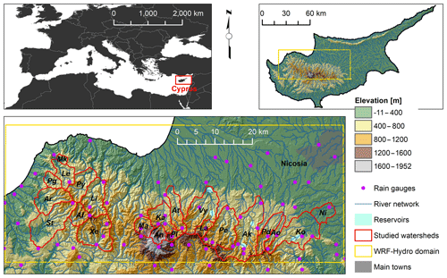
Figure 1Geographical setting of the island of Cyprus and WRF-Hydro study area with the 22 target watersheds. For watershed abbreviations refer to Table 1.
From this review, it appears that few studies focus on the evaluation of the hydrologic output of WRF-Hydro when forced with observed rainfall and just a few more when forced with modelled rainfall. Model performance loss due to differences between observed and modelled rainfall is rarely discussed. Also, little attention has been given to small watersheds (area below 100 km2), which are often ungauged and prone to flash floods. This study aims to address this gap. The focus is on two extreme events that occurred over 22 small watersheds, located in the Troodos Mountains of Cyprus, between 8–10 January 1989 and 20–22 November 1994. The main objectives are (i) to calibrate the uncoupled WRF-Hydro model for simulating extreme events in Cyprus with observed precipitation and (ii) to evaluate the model performance when forced with WRF-downscaled (1 km × 1 km) re-analysis precipitation data (ERA-Interim). The model runs covered two 15 d periods (1–16 January and 11–26 November) to include a short spin-up of the WRF-Hydro routines and the simulation and evaluation of the receding limb of the hydrograph.
This study focuses on 22 watersheds located on the northern slope of the Troodos Mountains, Cyprus (Fig. 1). The bedrock geology of the region is characterized by an ophiolitic complex. The highest peak of Troodos is Mt. Olympus (1952 m a.s.l.). At high elevations (above 1400 m a.s.l.), ultramafic rocks are the dominant lithology (harzburgite, serpentinite, pyroxenite, wehrlite and dunite). Moving downhill, dominant rock types show a transition from gabbro to diabase, pillow lavas and sedimentary formations, therefore stratigraphically from the lower to the higher lithotype. Between gabbro and pillow lavas, diabase is present in the form of sheeted dykes, and it constitutes the largest area of Troodos outcrop. Often, pillow lavas and sheeted dykes do not present a net geological limit, but the oldest lavas host the youngest dykes (Cleintaur et al., 1977). This transitional zone between pillow lavas and dykes takes the name of basal group. Throughout the ophiolitic complex, bedrock is usually found at shallow depths. According to the digital soil map of Cyprus (Camera et al., 2017), most of the soils over Troodos are Lithic Leptosols with a stony gravelly texture and a predominant very shallow depth (0–10 cm), which can sometimes reach up to 100 cm. These characteristics highlight why rock fractures can be considered the main controlling factor for the region's subsurface hydrology.
Due to its characteristic Mediterranean climate, more than 90 % of a hydrologic year's (October–September) runoff from Troodos is produced between December and April. During the summer months, most rivers are completely dry (Le Coz et al., 2016). Due to their small areas and steep slopes, all watersheds have quite short times of concentration. Therefore, intense rainfall events lasting few hours can easily cause floods in the downstream plains.
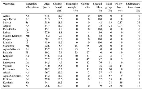
Table 1 lists the 22 watersheds, their area and the total modelled stream length, and it summarizes their geology, as obtained from the geological map of Cyprus (Cyprus Geological Survey Department, 1995). Agios Nikolaos and Platania are sub-watersheds of Kargiotis; Lagoudera is a sub-watershed of Vyzakia; Kotsiati is a sub-watershed of Nisou.
3.1 Streamflow data
For the 22 watersheds, daily discharge data (m3 s−1) from streamflow stations of the Cyprus Water Development Department for the period 1980–2010 were analysed. In addition, the original continuous hydrograph charts (water levels) of 16 of the 22 streamflow stations, for the January 1989 and November 1994 events, were scanned and manually digitized through the GetData Graph Digitizer software (http://getdata-graph-digitizer.com, last access: 21 October 2020). The digitized water levels were interpolated to obtain values precisely every 15 min (00.00, 00.15, 00.30, 00.45, 01.00 …) and converted to discharge with the appropriate rating curve of the station. The streamflow stations and rating curves are maintained by the Water Development Department through frequent observations. Both interpolation and conversion were carried out by R scripts (https://www.r-project.org/, last access: 21 October 2020). The 15 min data were aggregated into hourly discharge values. Both hourly and daily values were used for model performance analysis.
3.2 Meteorological data
An hourly gridded dataset with a resolution of 1 km × 1 km was developed using hourly and daily rainfall data from the Cyprus Department of Meteorology stations and the daily gridded rainfall dataset of Camera et al. (2014). Data were extracted for two extreme events, with 42 rain gauges available over the island for January 1989 and 37 rain gauges available for November 1994. The temporal disaggregation from daily to hourly gridded rainfall was developed through a FORTRAN code based on the method of hourly fractions (Di Luzio et al., 2008), which preserves the original daily values. The main steps of the disaggregation method are
- a.
The hourly rainfall observations (ph) are summed in 24 h totals (phs). The 24 h period ranges from 08:00 UTC+2 of the previous day until 08:00 UTC+2 of the attribution day, coherently with the daily gridded dataset.
- b.
The fractions of the hourly rainfall data to the daily total rainfall are calculated as
- c.
The nearest gauge to each rainfall gridded dataset cell (ng) is found.
- d.
The hourly rainfall at each grid cell (phc) is calculated by multiplying each gridded daily (d) rainfall value (pdc) with the hourly (h) fraction (hfrac) of the nearest valid gauge (ng).
4.1 WRF-Hydro model description
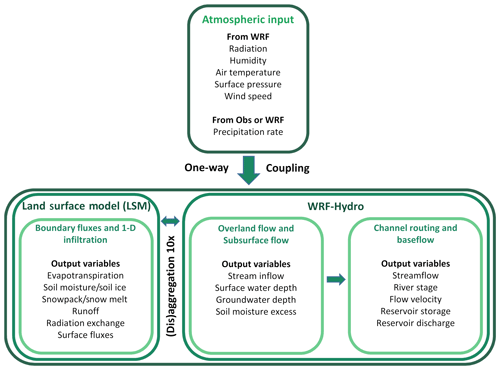
The WRF-Hydro model is an extension package of the 1-D Noah LSM and Noah-MP LSMs, which are commonly coupled to WRF. In this study, the Noah LSM 2.7.1 version and the WRF-Hydro 3.0 version, as modified by Rummler et al. (2019), were used. WRF-Hydro, in comparison to the traditional 1-D LSM, enhances the physical description and mathematical resolution of surface and near-surface hydrologic processes. It includes physics options for quasi 3-D saturated subsurface flow, 1-D or 2-D surface overland flow, 1-D channel routing, lake/reservoir routing, and baseflow processes. WRF-Hydro uses a disaggregation–aggregation procedure to resolve the hydrologic processes at a finer resolution than the LSM. Below, a brief description of the main modelled processes and characteristics is presented. For a detailed description of the model components the reader can refer to Gochis et al. (2015). A schematic representation of the model structure, as used in this study, is presented in Fig. 2.
One of the major advances of WRF-Hydro is the lateral subsurface flow component, which is calculated following the approach proposed by Wigmosta et al. (1994) and Wigmosta and Lettenmaier (1999). When precipitation reaches the surface, it can either infiltrate or run off. The partitioning between infiltration and runoff is controlled, besides the antecedent soil moisture conditions, by soil properties. In the Noah-LSM, the infiltration capacity (DDT) is defined as a function of the soil moisture deficit (DD) and an exponential scaled adjustment (VAL), which is a function of the parameter KDT. It follows the approach of Schaake et al. (1996), with the difference that KDT is not directly calibrated but is expressed as a function of the saturated hydraulic conductivity and two scaling coefficients:
where DT is the time step duration (d), Ks (m s−1) is the saturated hydraulic conductivity, REFDK is the reference (silty clay loam) saturated hydraulic conductivity (default 2×10⁶ m s−1) and REFKDT is the infiltration partitioning scaling coefficient, which needs to be calibrated to empirically correct KDT for natural variability. As was demonstrated by previous studies (e.g. Naabil et al., 2017; Verri et al., 2017; Givati et al., 2016; Senatore et al., 2015), the model is sensitive to REFKDT. Once the water enters the soil, it moves vertically, through a four-layer soil column, until it reaches the saturated level and then laterally, according to the local gradient. In case the moisture content at the top of the soil column is larger than its water holding capacity (saturation), exfiltration occurs. The exfiltration amount is added to the infiltration excess and is routed over the surface. At the bottom of the soil column a vertical flux is calculated, using the Richards equation (Richards, 1931). Drainage from the soil column is computed by multiplying the vertical flux with the SLOPE parameter, which can vary between 0 and 1, where 0 represents an impermeable boundary between the soil column and the underlying formations. The SLOPE parameter is assigned based on terrain slope classes through a table; however in an implicit way it expresses bedrock properties too (the higher the slope, the higher the SLOPE coefficient in order to scale the projected map area over which deep drainage occurs). Drained water can be considered a loss or added to streamflow within the channel network through a conceptual baseflow module, if this is activated.
Regarding overland flow, WRF-Hydro allows water to pond on the earth's surface. A water retention depth is defined based on land use and vegetation cover. This parameter can be adjusted through a scaling factor (RTDPT), which can be specified for each model cell and can vary between 1 and 10 (Yucel et al., 2015). The fraction of ponded water exceeding the retention depth is available to overland flow routing. The routing is performed based on the diffusive wave formulation of Julien et al. (1995) and it can be resolved in both 1-D (Steepest Descent) and 2-D (x–y directions). Overland roughness is defined through the same tables as the retention depth, and it can be adjusted through the overland-roughness routing factor (OVRGH), which can vary between 0 and 1 (Yucel et al., 2015). Overland flow can re-infiltrate, evaporate or enter the channel network.
Water entering the channel network, which the user defines through a digital elevation model, is routed based on a streamflow algorithm that uses an implicit, one-dimensional, variable time-stepping diffusive wave formulation. Such a formulation is a simplification of the St. Venant equations for shallow water flow. The algorithm does not allow overbank flow and therefore the 2-D modelling of floods (Rummler et al., 2019). Channels are considered trapezoidal in section. Their geometrical properties, including roughness, are defined based on stream order. These model parameters are entered through a table and they can be set by expert knowledge or adjusted during calibration. Along the channel network, reservoirs can be added. Water can flow into reservoirs through the channel network or when overland flow intersects them. Water can flow out of the reservoir through weir overflow and gate-controlled flow. These fluxes are governed by the reservoir parametrization (reservoir area, maximum water level in the reservoir, weir length, gate area, gate elevation, gate aperture coefficient). No exchanges occur between the reservoir, the atmosphere, and the soil column around the reservoir (i.e. evaporation and subsurface lateral flow from the reservoir are not accounted for).
When deep drainage from the soil column is not considered as a loss, WRF-Hydro allows two simple mathematical solutions to account for baseflow. For both solutions, baseflow is calculated within sub-watersheds. The first solution consists of a simple pass-through model, meaning that the cumulated deep drainage occurring in a time step is equally redistributed to all channel segments within the sub-watershed. The second solution consists of calculating a baseflow discharge (m3 s−1) (Qbf) by means of an exponential bucket model, described by the following equation:
where C is the bucket coefficient (m3 s−1), a is the bucket model exponent (–), Zmax is the maximum bucket level (m) and Z (m) is the bucket level at a certain time step. The user defines the C, a and Zmax parameters for each sub-watershed, together with a Zini (m) parameter to initialize the water storage in the bucket groundwater reservoir. At each time step the Z value is updated first, adding the deep-drainage contribution (Perc) and subsequently subtracting Qbf:
where A is the area of the sub-watershed (m2), DT the model time step (d), n the index for the sub-watershed cells and ncells the number of cells of the sub-watershed. Similar to the first solution, Qbf is equally redistributed to channel segments. If Z equals or exceeds Zmax, all deep drainage is transferred to the channel network.
4.2 WRF-Hydro model parameterization
The Noah LSM was parameterized over a 1 km × 1 km grid, while WRF-Hydro was run over a 100 m × 100 m grid. All simulations were performed in an uncoupled mode, resolving the steepest descent formulation of the overland flow routine, with channel flow, baseflow and reservoir routines activated.
To run WRF-Hydro in the uncoupled mode, the meteorological forcings needed are precipitation rate (mm s−1), downward shortwave and longwave radiation (W m−2), specific humidity (kg kg−1), air temperature (K), surface pressure (Pa), and near-surface wind components (m s−1). For the calibration and validation runs, all variables except precipitation were taken from the WRF ERA-Interim downscaling experiments presented in Zittis et al. (2017). These simulations incorporated the Grell–Freitas ensemble convection and the Ferrier microphysics parameterization schemes, which were found to outperform the other tested configurations for the selected events. For precipitation, hourly observed gridded data were used (see Sect. 3.2 – Meteorological data). For the simulation runs with WRF-modelled rainfall, all variables including precipitation were taken from the WRF experiments (Zittis et al., 2017). To derive soil moisture initial conditions, 15 d WRF spin-up runs were performed for both events. For January 89, the 15 d rainfall during spin-up was 99 mm, and average soil moisture at the end of the simulation was 0.32 m3 m−3. The November 1994 event followed the dry summer, and only a few scattered rain days occurred between the end of October and the beginning of November. The 15 d rainfall during spin-up was 18.4 mm, and average soil moisture at the end of the simulation was 0.26 m3 m−3. Experimental data (Camera et al., 2018) show that in these conditions soil moisture for a gravelly sandy loam at 1300 m a.s.l. in the Troodos Mountains can vary between 0.10 and 0.15 m3 m−3. Therefore, the WRF-derived initial soil moisture values for November were halved.
Land use and vegetation cover data were derived from the MODIS dataset through the WRF Pre-Processing System. According to the MODIS dataset, the Troodos Mountains have a uniform clay loam texture. However, field observations at higher elevation in the mountains, where the predominant lithologies consist of gabbro and ultramafic rocks, showed a gravelly sandy loam texture (Djuma et al., 2020; Camera et al., 2018; Cyprus Geological Survey Department, 1995). In addition, it is known that the Troodos gabbro is very weathered and therefore permeable (Christofi et al., 2020). Therefore, a sandy loam soil type was assigned to these areas. The related properties were attributed through the default table values implemented in WRF-Hydro (see Gochis et al., 2015). The hydrologic input layers (latitude, longitude, topography, flow direction, channel grid, lake grid, stream order, watersheds) were all calculated in ArcGIS® 10.2.2 starting from a 25 m × 25 m digital elevation model (see Camera et al., 2017), resampled on the 100 m × 100 m grid and the known locations of stream gauges and lakes. For the channel grid, a flow accumulation threshold of 250 cells (2.5 km2) was adopted.
For the definition of the deep-drainage-related parameter, two approaches were tested. First, nine slope terrain classes were derived following Silver et al. (2017). In the second case, for cells where the bedrock consists of gabbro or ultramafic rocks (Cyprus Geological Survey Department, 1995), the slope terrain class (3) that maximizes drainage (representing a highly fractured system) was assigned. In both cases, for each slope terrain class, the related default SLOPE value listed in the WRF-Hydro general parameter table was given. These changes in soil type and deep drainage based on geology affected mainly watersheds Ma, An, Pl, Ka and At, where 70 % or more of the surface bedrock is made up of gabbro and ultramafic rocks (Table 1).
Other general parameters are REFKDT and soil depth (SD), which were calibrated. REFDK was left to its default value ( m s−1). The WRF-Hydro parameter OVRGH was tested and values were assigned based on the sensitivity analysis, whereas RTDPT was kept constant all over the study area, and a value of 1, consistent with a steep mountainous terrain, was assigned.
Channel geometrical parameters were attributed based on the study area knowledge of the authors (Table 2). The initial channel water depth was set to the default value for dry conditions. Six reservoirs were characterized in the model set-up (Table 3) according to data from the Cyprus Water Development Department (2009). At all reservoirs, outflow occurs for overflow only; the structures do not have a gate. Vyzakia reservoir was completed in early 1994; therefore it was not included in the January 1989 simulation.
Table 2WRF-Hydro channel parameter values used in this study (Bw is the channel bottom width, HLINK is the initial depth of water in the channel, ChSSlp is the channel side slope and MannN is the Manning's roughness coefficient).
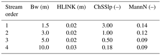
Table 3Characteristics of the reservoirs included in the WRF-Hydro simulations; Long and Lat are longitude and latitude, respectively.

Regarding baseflow, the parameter C was set equal to the long-term baseflow index, calculated from the 1980–2010 data series with the program PART (Rutledge, 1988). The initial level of the conceptual reservoir (Zini) was set as a fraction of the maximum level (Zmax), based on the saturation degree of the deepest soil layer at the end of the 15 d WRF spin-up period. The exponents a and Zmax were adjusted during calibration.
4.3 WRF-Hydro sensitivity analysis
A sensitivity analysis of the LSM parameters REFKDT, SLOPE, and soil depth (SD), which have been identified as sensitive parameters in previous studies (e.g. Fersch et al., 2019; Senatore et al., 2015), was performed for the January 1989 event. In addition, sensitivity runs for the OVRGH parameter and the saturated hydraulic conductivity (Ks) were performed, too. For these simulations, the baseflow routine was switched off. A reference scenario was set, with REFKDT and OVRGH equal to 1, SD equal to 1.0 m, Ks equal to m s−1 (value attributed to clay loam soils in the soil parameter table) and the deep-drainage parameter (SLOPE) assigned based on terrain slope, as in Silver et al. (2017). Parameters were changed one at a time. Eight values were tested for REFKDT (0.3, 0.5, 3.0, 5.0, 8.0, 10.0, 100.0, 1000.0) and two for SD (0.5 and 2.0 m), two for OVRGH (0.1, 0.5), three for Ks ( m s−1 as for loam, m s−1 as for sandy loam, m s−1 as for loamy sand), and a different set of SLOPE values was assigned based on terrain slope and geology. Also, to demonstrate the equifinality of calibrating REFDK and REFKDT, as suggested by Eq. (5), two extra runs were performed for REFDK values of and m s−1. The relative sensitivity (S) was computed according to the following formula:
where Vtot is the total volume discharged during the simulation period, ref refers to the reference scenario, and i is the perturbed value.
4.4 WRF-Hydro calibration and validation with observed precipitation
Calibration runs were evaluated for each watershed against January 1989 daily observed streamflow, based on five performance indices. The selected set of indices contains both absolute error and goodness-of-fit measures, as suggested by Legates and McCabe (1999). They are percent bias (PBIAS), mean absolute error (MAE), Nash–Sutcliffe efficiency (NSE – Nash and Sutcliffe, 1970), modified Nash–Sutcliffe efficiency (mNSE; Krause et al., 2005) and Kling–Gupta efficiency (KGE; Kling et al., 2012).
Soil depth is constant throughout the domain; therefore it was fixed at the value that returned the best performance indices in the majority of the watersheds, following an evaluation of the sensitivity analysis runs. Similarly, SLOPE parameters were assigned using the slope terrain class map allowing the best performance during sensitivity. REFKDT and OVRGH were initialized, in each watershed, based on the evaluation of the sensitivity runs through performance indices, as for SD. For the baseflow bucket routine, initial values of α and Zmax were set to the default. Next, the initialized parameters were fine-tuned based on a trial-and-error procedure for all watersheds. Modifications were applied to a single parameter at the time, and if changes could not improve the model performance according to three indices out of five after five attempts, the parameters were retained. Commonly applied changes were ±1 for REFKDT, ±0.1 for OVRGH, ±0.5 for α and ±10 % of the actual value for Zmax. Smaller (larger) changes were applied only in watersheds where the response of streamflow was (not) particularly sensitive to specific parameters. The parameterization of Zmax was aimed at filling the reservoir after the rainfall peak, between 10 January at midnight and 11 January at noon, to simulate the observed recession of the hydrograph. For those watersheds that highly overestimated the baseflow due to spilling out of the groundwater reservoir, Zmax was further increased. A good fit between observed and simulated flow before the peak was the target for the calibration of the exponent α. The calibrated model was subsequently applied to the November 1994 event for validation. The same five model performance indices were used for the evaluation.
4.5 WRF-Hydro simulations with WRF-modelled precipitation
The WRF-modelled precipitation (Zittis et al., 2017) was averaged over each of the 22 watersheds, and the daily values were compared to observed data by means of BIAS, MAE and NSE. To evaluate how deviations from the observed rainfall pattern affected the hydrologic model performance in these small mountain watersheds, the calibrated version of the WRF-Hydro model was run with the WRF-modelled hourly precipitation forcing. Modelled streamflow was evaluated with observed data, similar to in the calibration phase.
4.6 WRF-Hydro evaluation with observed and modelled precipitation at an hourly scale
For watersheds presenting daily NSE equal to or larger than 0.50 for both the calibration and the validation event, model performance was also investigated at hourly resolution. The NSE, KGE and MAE were computed for the hourly streamflow values simulated with both observed and modelled precipitation.
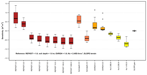
Figure 3Boxplots of the sensitivity of the modelled streamflow to perturbations (x axis) in REFKDT (infiltration partitioning scaling coefficient), soil depth, OVRGH (overland roughness factor), Ks (saturated hydraulic conductivity) and SLOPE geo (deep-drainage parameter defined based on slope terrain and geology) relative to a defined reference scenario (SLOPE terrain represents the slope parameter defined based on slope terrain only, as in Silver et al., 2017).
5.1 Sensitivity analysis
The results of the sensitivity analysis are presented in Fig. 3 as boxplots. Each boxplot represents the sensitivity of the modelled total discharge volume, over the 22 watersheds, for the perturbation applied, in comparison to the reference simulation. The boxplots show that in the suggested calibration range (0.5–5.0; Gochis et al., 2015) REFKDT is very sensitive. Although the sensitivity decreases for REFKDT values larger than 5.0, variations in the discharged volume can be observed up to REFKDT values equal to 100.0. Further increases in REFKDT (see REFKDT 1000.0) do not cause any variations in discharge, suggesting that the model already infiltrates at its maximum capacity. The variability over the watersheds is related to local conditions (e.g. soil moisture distribution, area, topography, type of vegetation). Precipitation, which is not homogeneous throughout the study area, can play a role in causing different responses as well.
The two simulations run with REFDK values of and m s−1 returned discharged volumes equal to those obtained with REFKDT values of 0.5 and 3.0, respectively. These results confirm the equifinality of the two parameters and make it clear that REFDK calibration should be avoided. As shown in Eqs. (3)–(5), REFDK automatically adjusts the infiltration capacity for the effect of soil texture, whereas any other effects on the partitioning of rainfall into surface runoff and infiltration can and should be calibrated through REFKDT.
The sensitivity analysis also shows an important role played by soil depth. Especially in mountainous areas, soils are usually thin. This limited soil thickness affects the total amount of water retained by the soil, favouring a partitioning of the available water between infiltration and surface runoff towards the latter. Similar observations are reported by Fersch et al. (2019), while commenting on the offset between modelled and observed soil moisture content in mountainous catchments in Bavaria (Germany). To overcome the issue, in other land surface models (e.g. Brunke et al., 2016) variable soil thickness has been implemented and tested.
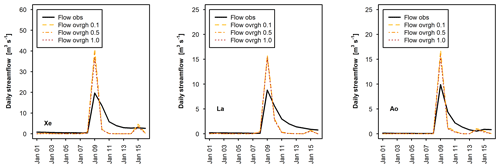
Regarding OVRGH, results show that it has a slight control on the total volume discharge, as also presented in Yucel et al. (2015), while it has almost no effect on delaying the peak (Fig. 4). More sensitive than OVRGH is Ks, suggesting a possible important impact of the soil type and property definitions on the model output. Senatore et al. (2015) presented one of the few WRF-Hydro studies that calibrated a hydraulic-conductivity-related parameter, although they focused on the saturated soil lateral conductivity. SLOPE appeared to have a low sensitivity, although in the mountain watersheds, where it changed, a small reduction in the total discharged volume was observed.
5.2 WRF-Hydro calibration and validation with observed precipitation
The calibrated parameters are listed in Table 4. Soil depth was set equal to 1 m for all watersheds, because it was the value returning the best performance indices (Fig. 4) in 16 out of 22 catchments (average NSE improvement equal to 0.14). SLOPE attributed based on both terrain slope and geology resulted in slightly better performance indices in the mountain watersheds than SLOPE attributed through terrain slope only. Therefore, it was selected for the final parameterization. Also, for all watersheds OVRGH was set equal to 1 because it was the value returning the best performance indices in 19 out of 22 watersheds. Furthermore, considering that OVRGH affects total discharge volume and not hydrograph shape, its calibration would have been equifinal to REFKDT. Twelve watersheds have a REFKDT coefficient larger than 5.0, which is outside the 0.5–5.0 range suggested by Gochis et al. (2015), but none have a REFKDT lower than 0.5. The hydrographs of all watersheds are shown in the Supplement. Figures S1 and S2 show hydrographs, including the baseflow component, related to responses to observed rainfall for the January 1989 event and the November 1994 event, respectively.
Table 4Calibrated parameters (REFKDT, infiltration partitioning scaling coefficient; C, baseflow bucket coefficient; α, bucket exponent; Zmax, maximum bucket level) for the 22 watersheds with their maximum (Max Q) and average (Ave Q) discharges for the two analysed events; for watershed abbreviations refer to Table 1.
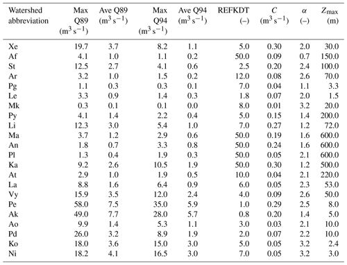
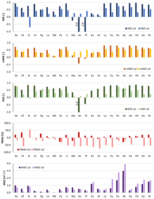
Figure 5Performance indices (NSE, Nash–Sutcliffe efficiency; mNSE, modified Nash–Sutcliffe efficiency; KGE, Kling–Gupta efficiency; BIAS; MAE, mean absolute error) calculated on daily streamflow resulting from observed rainfall for the 22 watersheds using the calibrated set of parameters for both January 1989 (cal) and November 1994 (val). For watershed abbreviations refer to Table 1.
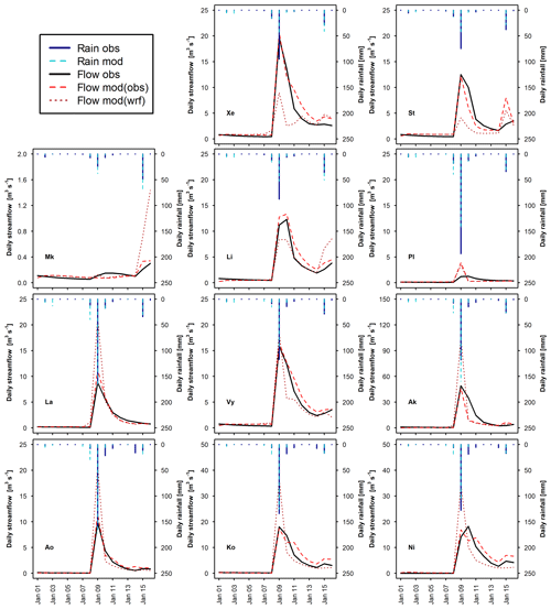
Figure 6Observed daily hydrographs (Flow obs) and hydrographs obtained with the calibrated WRF-Hydro model (Flow mod) forced with observed rainfall (Rain obs) and with WRF-modelled rainfall (Rain wrf) for the January 1989 calibration event, for 11 representative watersheds (see Table 1 for watershed abbreviations).
The parameterization of watersheds Ma, An, Pl, Ka and At is peculiar. These watersheds are mainly characterized by sandy loam texture (i.e. higher Ks than the other watersheds), maximum deep drainage obtained by using the SLOPE parameters based on slope terrain and geology, very high REFKDT values, and very large groundwater storage. However, poor model fit indices (for some watersheds even negative) were obtained for the calibration period (Fig. 5). Conversely, the same watersheds show positive NSE values and negative PBIAS (i.e. slight underestimation of the peak discharge), for the validation event. Overestimation of runoff in January 1989 could have been related to the modelling of snow and snowmelt in the LSM. Both observed and modelled temperature values for the upstream areas of these watersheds showed negative values, indicating that part of the precipitation was snow. In Fig. 6, the comparison between the observed and simulated daily hydrographs for the January 1989 event is shown. The subdued response of the streamflow to the extreme precipitation is clear for watershed Pl, which is considered representative of the behaviour of all five watersheds mentioned above, and it is clear that the simulated hydrograph overestimates the observed peak flow of the event. Different bottom boundary conditions and snow process modelling, as those implemented in the Noah Multi-Physics LSM, could improve the simulation results.
Overall, in all other watersheds the model behaves satisfactorily, with goodness-of-fit scores (NSE, mNSE and KGE, Fig. 5) usually higher than 0.5 for the calibration run and larger than 0.0 for the validation event. Exceptions are watershed Mk for the calibration run and watershed St for the validation run. Looking at the hydrographs (Figs. 6 and 7), it is observed that Mk presents a very low discharge due to its limited area (Table 4). Therefore, small biases between observed and modelled streamflow produce poor goodness-of-fit indices. Also, Mk is the only watershed showing higher rainfall and flow peaks towards the end of the January 1989 event rather than in the middle. The model slightly underestimates the flow peak that occurred on 9 January and overestimates the flow at the end of the simulation period. For St, the model reacts sharply to precipitation input, simulating the flow peak that occurred on 9 January well but overestimating the flow at the end of the simulation period of the January 1989 event and above all the peak of the November 1994 event, therefore affecting the performance scores.
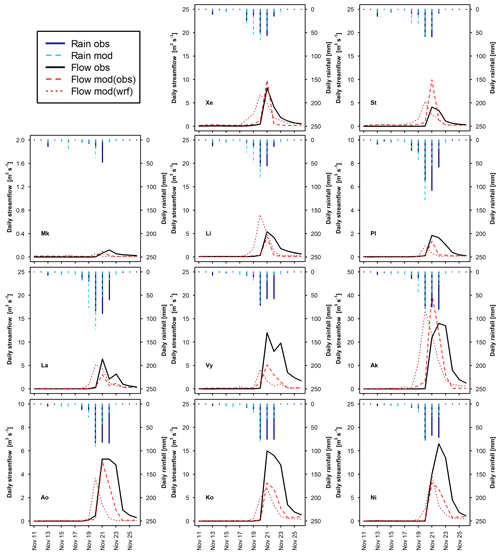
Figure 7Observed daily hydrographs (Flow obs) and hydrographs obtained with the calibrated WRF-Hydro model (Flow mod) forced with observed rainfall (Rain obs) and with WRF-modelled rainfall (Rain wrf) for the November 1994 validation event, for 11 representative watersheds (see Table 1 for watershed abbreviations).
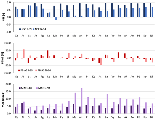
Figure 8Performance indices (NSE, Nash–Sutcliffe efficiency; BIAS; MAE, mean absolute error) of daily WRF-modelled rainfall over the 22 watersheds for both January 1989 (J-89) and November 1994 (N-94) events. For watershed abbreviations refer to Table 1.
In the eastern part of the modelling domain (La to Ni), for the calibration event both initial baseflow and the discharge peak are well modelled in all watersheds (Fig. 6). Differences between observed and simulated hydrographs can be observed in the post-peak, for watersheds Ak, Pe (Fig. S1), Ko and Ni. Ak and Pe present a very high peak flow (>50 m3 s−1) and an underestimation of the receding limb of the hydrograph in the following days, which causes the negative PBIAS and high MAE values visible in Fig. 5. In the case of Ko and Ni, the receding limb shows a little overestimation. For the validation event (Fig. 7), the peak is well simulated in Pe and Ao, slightly overestimated in Ak and Pd, and underestimated in La, Vy, Ko, and Ni (Pe and Pd, Fig. S2). In the post peak phase, the simulated hydrographs show negative biases in comparison to the observed ones in all watersheds. As is visible in Figs. S1 and S2 in the Supplement, flow in the receding limb of the hydrograph is mainly made up of baseflow. For the January 1989 event, in all these watersheds the groundwater reservoir fills up on 10 January and baseflow consists of the water spilling out from it. This water volume, redistributed along the channel network, is generally able to reproduce the hydrograph shape, except in Ak. In November 1994, no groundwater spilling is observed during the simulation and the receding limb is underestimated. Therefore, this could be partly due to a non-perfect reproduction of the model initial conditions and partly related to an underestimation of interflow and baseflow.
5.3 WRF-Hydro simulations with modelled precipitation
Figure 8 presents the performance indices of the WRF-modelled rainfall. Figures S3 and S4 show hydrographs, including the baseflow component, related to responses to modelled rainfall for all watersheds for the January 1989 event and the November 1994 event, respectively. The modelled rainfall is generally closer to observations for the January 1989 event than for the November 1994 event, as testified by the higher NSE (except for Le) and lower MAE values (Fig. 8). As can be seen in Fig. 6, the January 1989 event appears as a single day of intense precipitation, followed by a few scattered low-rainfall days that can show a moderate intensity towards the end of the simulation period. During January 1989, WRF-modelled rainfall is usually able to fit the observed daily precipitation trend over all watersheds, with slight variations in the calculated daily amounts as suggested by the generally low bias (Fig. 8). In percentage, over the 22 watersheds rainfall PBIAS varies between −35 % and 53 %, with an average of absolute values equal to 17 %. Average NSE and MAE of the WRF-modelled rainfall are 0.83 and 4.5 mm d−1, respectively.
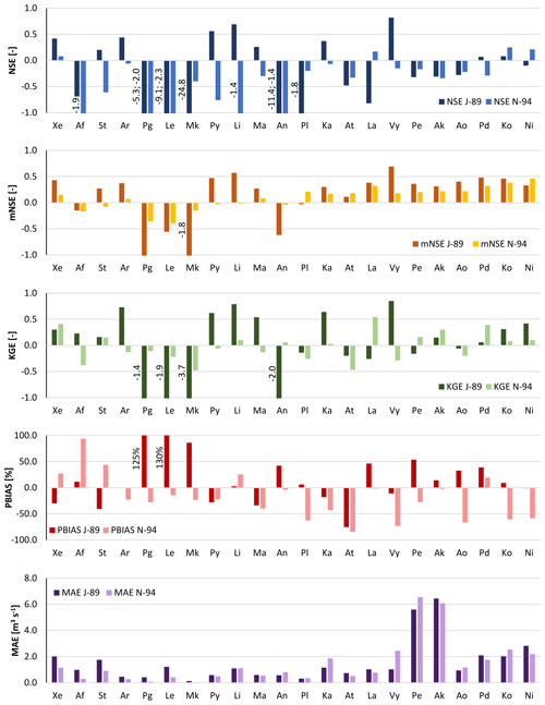
Figure 9Performance indices (NSE, Nash–Sutcliffe efficiency; mNSE, modified Nash–Sutcliffe efficiency; KGE, Kling–Gupta efficiency; BIAS; MAE, mean absolute error) calculated on daily streamflow resulting from WRF-modelled rainfall for the 22 watersheds using the calibrated set of parameters for both the January 1989 (J-89) and November 1994 (N-94) events. For watershed abbreviations refer to Table 1.
Figure 7 shows that the November 1994 event is constituted of 2 d of moderately low precipitation, followed by 3 d of intense precipitation. The simulated event shows higher rainfall amounts in the preceding days and a loss of intensity after the first of the three high-precipitation days. Over the 22 watersheds, average NSE, absolute PBIAS and MAE are 0.48, 20 % and 8.9 mm d−1, respectively.
The modelled rainfall in January 1989 results in hydrograph shapes similar to the observed ones but still in goodness-of-fit indices that are often negative. With observed rainfall forcing, the simulated daily hydrograph returned negative NSE, mNSE and KGE values (Fig. 5) in three, two and two watersheds, respectively. With WRF-modelled rainfall forcing, the number of watersheds with negative indices (Fig. 9) increases up to 12, 6 and 9, respectively. Moving from observed to WRF-modelled rainfall, both streamflow NSE and MAE indicate a loss in model performance in all watersheds except three (Ma, Pl, Ka), which are those characterized by very negative goodness-of-fit indices in the calibration run. The average streamflow MAE almost doubled, and ranged between 0.09 m3 s−1 in Mk and 3.89 m3 s−1 in Pe. The absolute value of flow PBIAS decreased in seven watersheds (Af, Li, Pl, Vy, Ak, Ko, Ni) but on average increased by 21.5 % (96.6 % in Pg and 120.3 % in Le).
Regarding streamflow for the November 1994 event, the peak discharge is simulated to occur 1 d earlier than observed in most watersheds. This caused negative streamflow performance indices in 18 watersheds for NSE, in eight watersheds for mNSE and in 11 watersheds for KGE (Fig. 9), while with the forcing of observed rainfall, negative indices were found in one, zero and three watersheds, respectively (Fig. 5).
These results indicate that a small shift in time or space of modelled rainfall, in comparison to observed precipitation, can strongly modify the hydrologic response of small watersheds to extreme events. This is particularly evident in watersheds Pg and Mk, which are among the smallest and those characterized by the lowest average discharge in both events (Figs. 6, 7, S3 and S4). Although their rainfall performance indices (Fig. 8) do not show particularly large errors (except a negative NSE for Mk in November 1994), streamflow fit indices present very negative values and streamflow PBIAS is very high as well (Fig. 9).The implementation of rainfall data correction or assimilation schemes could improve the forecasts of the atmospheric–hydrologic modelling chain, as demonstrated and discussed by previous studies (e.g. Avolio et al., 2019; Verri et al., 2017; Yucel et al., 2015). Recently, increasing efforts have been made to implement two-way-coupled modelling systems, which were found to improve the overall skills of the modelling system (e.g. Senatore et al., 2015). However, the hydrologic component calibration is still usually performed based on observed precipitation data (e.g. Fersch et al., 2019; Givati et al., 2016).
The rainfall fields modelled by Zittis et al. (2017) and used in this study were downscaled from the ERA-Interim re-analysis dataset. The decision to use these modelled data was driven by the fact that ERA-Interim presents a resolution closer to that of existing forecasting, decadal prediction and global climate models; therefore it resembles a modelling chain for forecasting applications and climate change projections (e.g. Reyers et al., 2019; Saha et al., 2014). For future studies, ERA5, thanks to its finer resolution and the availability of ensemble members for uncertainty estimates, will be a valuable data source for improving the modelling chain over small (<100 km2) catchments.
5.4 WRF-Hydro with observed and modelled precipitation evaluation at an hourly scale
Figure 10 shows the comparison between observed and modelled hourly hydrographs for three out of the seven watersheds that had modelled daily streamflow NSE larger than 0.5 in both calibration and validation events. The four watersheds that are not shown are Pg (hourly streamflow data not available), Pe, Ko and Ni (rating curve not available for peak flow). Looking at the streamflow modelled with observed rainfall as forcing, hourly peaks are generally overestimated and the modelled streamflow response to rainfall appears more immediate (pulse-like) than the observed streamflow. The overestimation is more evident for the November 1994 validation event than for the January 1989 calibration event. In addition, the receding hydrograph is well modelled for the calibration event but not so well for the validation event. This result is similar to what was observed for daily streamflow and was attributed to the possible non-perfect reproduction of the model initial conditions and underestimation of interflow. The fairly good post-peak simulations lead to reasonable hourly performance indices for the January 1989 event. However, even with an NSE of 0.80 and a KGE of 0.72 for watershed Ao, the 17.9 m3 s−1 hourly peak flow was overestimated by 18 %.
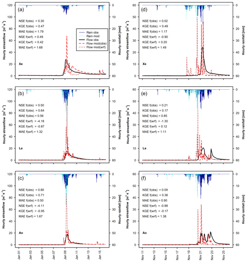
Figure 10Observed hourly hydrographs (Flow obs) and hydrographs obtained with the calibrated WRF-Hydro model (Flow mod) forced with observed rainfall (Rain obs) and with WRF-modelled rainfall (Rain wrf) for both January 1989 (a–c) and November 1994 (d–f), for three watersheds (see Table 1 for watershed abbreviations); modelled flow performance indices (NSE, Nash–Sutcliffe efficiency; KGE, Kling–Gupta efficiency; BIAS) are shown as well.
The response of hourly streamflow to WRF-modelled rainfall shows similar behaviour. The shape of the hydrographs is defined by rainfall pulses, in terms of both time of response and size of peaks. Even more than for daily outputs, it is evident that small differences in rainfall distribution and amount can cause large differences between observed and modelled streamflow (see performance indices).
A possible improvement may be obtained by an increase in channel roughness coefficients. This would allow slower flow and a smoothing of the peaks. Especially in dry Mediterranean areas, characterized by streams with seasonal flow, the vegetation (and consequently the roughness conditions) can be very different at the end of the dry period (vegetation grown within the stream, dry understoreys and bushes, and bare cropland overland) and in the middle of wet winter (water within the riverbed, green vegetation cover overland). This could be described with the inclusion of a seasonal variation in channel and overland roughness coefficients in the model. However, rainfall data with high spatial and temporal resolution would be essential to test this model modification.
This study evaluates streamflow simulations of the one-way-coupled atmospheric–hydrologic model WRF-Hydro, forced with observed and WRF-modelled rainfall, during two extreme events, over 22 small mountain watersheds in Cyprus (area below 100 km2). Following model calibration and validation with observed rain, the model was run with WRF-downscaled (1 km × 1 km) re-analysis precipitation data (ERA-Interim). These forcing data represent best-performing hindcasts of two extreme rainfall events, i.e. a model product that is as similar as possible to reality and considered sub-optimal.
Overall, the selected four calibration parameters (REFKDT, soil depth, the baseflow bucket exponent and the maximum baseflow bucket capacity) were sufficient to obtain good model performance during model calibration in these steeply sloping and geologically complex watersheds. Sensitivity analysis showed that REFKDT can be calibrated beyond the suggested 0.5–5.0 range, having an effect on infiltration till a value of approximately 100.0. A soil depth of 1.0 m, representative of the thin soils characterizing the study area, rather than the default value of 2.0 m, resulted in an average increase in NSE values of 0.14. Modifications of deep-drainage coefficients and MODIS soil types based on geology reduced the peak flow overestimation by up to 40 % in watersheds characterized by a fractured and very permeable bedrock. The overland roughness routing factor reduced the streamflow but showed a very limited effect on delaying flow. A straightforward calibration of the baseflow reservoir based on low flow fitting (exponent) and reservoir filling time (maximum capacity) was a good mean for obtaining a reasonable simulation of the hydrograph recession in most watersheds. Calculated daily NSE values were higher than 0.5 in 16 out of the 22 modelled watersheds in January 1989 (calibration) and in eight watersheds in November 1994 (validation). Negative NSE values were found in three watersheds located at high elevation where an underestimation of the snow fraction, computed by the LSM, may have occurred. Modelled snow height, and possible improvements deriving from the use of alternative routines (e.g. Noah MP), should be checked with observed snow depth data, which were not available for this study.
The comparison of modelled and observed hourly streamflow showed that almost all peak flows were overestimated by the calibrated model. Modelled hourly streamflow fit the January 1989 hydrographs relatively well, but much less so the November 1994 discharges. This performance loss in November 1994 was due to a pulse-like behaviour of the modelled streamflow related to an immediate response to rainfall, which could be attenuated by higher channel roughness coefficients.
Streamflow obtained with WRF-modelled rainfall forcing showed high discrepancies with observations, despite the good agreement between modelled and observed precipitation (average NSE of 0.83 and 0.49 for January 1989 and November 1994, respectively). However, the relatively small errors in total precipitation (average relative difference over the 22 watersheds of 17 % and 20 % for the January 1989 and November 1994 events, respectively) and simulated daily maxima (average relative difference over the 22 watersheds of 22 % and 18 % for the January 1989 and November 1994 events, respectively) indicate that modelled rainfall data could be suitable for investigating the effect of climate change on extreme rainfall and flood events. From the results presented and discussed, it emerges that future studies could focus on various aspects of the modelling system to improve the simulation results of both precipitation and streamflow. Soil properties could be specifically calibrated for the study area. For a continuous, long-term streamflow analysis, an evaluation of the sensitivity of the baseflow reservoir parameters could be carried out. Also, the model could be improved by incorporating an option for time-dependent roughness coefficients to represent vegetation growth in ephemeral and intermittent streams in semi-arid environments. A model configuration with variable soil depths could also improve model performance, especially in mountain environments.
WRF-Hydro is an open-source community model (https://ral.ucar.edu/projects/wrf_hydro/overview, last access: 21 October 2020) (UCAR, 2020). WRF-Hydro-simulated streamflow at the watershed outlets, for the two events (January 1989 and November 1994) and the two forcings (observed and modelled precipitation), is available online at https://doi.org/10.5281/zenodo.3952420 (Camera et al., 2020).
The supplement related to this article is available online at: https://doi.org/10.5194/nhess-20-2791-2020-supplement.
CC, AB and GZ conceptualized the study. CC and AB developed the methodology. CC conducted the WRF-Hydro simulations with support from IS and the supervision of JA. GZ, CC and IS pre-processed the modelled and observed atmospheric input. CC, IS and AB digitalized the streamflow data. CC processed and analysed the model outputs with support from IS. CC prepared the original draft with contributions from all authors. AB was responsible for funding acquisition and supervised the project.
The authors declare that they have no conflict of interest.
This article is part of the special issue “Integrated assessment of climate change impacts at selected European research sites – from climate and hydrological hazards to risk analysis and measures”. It is not associated with a conference.
For computation, this work was supported by the Cy-Tera Project (NEA ΥΠOΔOMH/ΣTPATH/0308/31), which is co-funded by the European Regional Development Fund and the Republic of Cyprus through the Research Promotion Foundation. Authors would also like to thank the Water Development Department of Cyprus for data sharing and support.
This research has been supported by the BINGO project (Bringing INnovation to onGOing water management) and European Union's Horizon 2020 Research and Innovation programme (grant no. 641739).
This paper was edited by Beniamino Russo and reviewed by two anonymous referees.
Arnault, J., Wagner, S., Rummler, T., Fersch, B., Bliefernicht, J., Andresen, S., and Kunstmann, H.: Role of runoff–infiltration partitioning and resolved overland flow on land–atmosphere feedbacks: A case study with the WRF-hydro coupled modeling system for West Africa, J. Hydrometeorol., 17, 1489–1516, https://doi.org/10.1175/JHM-D-15-0089.1, 2016.
Arnault, J., Wei, J., Rummler, T., Fersch, B., Zhang, Z., Jung, G., Wagner, S., and Kunstmann, H.: A joint soil-vegetation-atmospheric water tagging procedure with WRF-Hydro: Implementation and application to the case of precipitation partitioning in the upper Danube river basin, Water Resour. Res., 55, 6217–6243, https://doi.org/10.1029/2019WR024780, 2019.
Avolio, E., Cavalcanti, O., Furnari, L., Senatore, A., and Mendicino, G.: Brief communication: Preliminary hydro-meteorological analysis of the flash flood of 20 August 2018 in Raganello Gorge, southern Italy, Nat. Hazards Earth Syst. Sci., 19, 1619–1627, https://doi.org/10.5194/nhess-19-1619-2019, 2019.
Brunke, M. A., Broxton, P., Pelletier, J., Gochis, D., Hazenberg, P., Lawrence, D. M., Leung, L. R., Niu, G.-Y., Troch, P. A., and Zeng, X.: Implementing and evaluating variable soil thickness in the community land model, Version 4.5 (CLM4.5), J. Climate, 29, 3441–3461, https://doi.org/10.1175/JCLI-D-15-0307.1, 2016.
Camera, C., Bruggeman, A., Hadjinicolaou, P., Pashiardis, S., and Lange, M. A.: Evaluation of interpolation techniques for thecreation of gridded daily precipitation (1×1 km2); Cyprus, 1980–2010, J. Geophys. Res.-Atmos., 119, 693–712, https://doi.org/10.1002/2013JD020611, 2014.
Camera, C., Zomeni, Z., Noller, J. S., Zissimos, A. M., Christoforou, I. C., and Bruggeman, A.: A high resolution map of soil types and physical properties for Cyprus: A digital soil mapping optimization, Geoderma, 285, 35–49, https://doi.org/10.1016/j.geoderma.2016.09.019, 2017.
Camera, C., Djuma, H., Bruggeman, A., Zoumides, C., Eliades, M., Charalambous, K., Abate, D., and Faka, M.: Quantifying the effectiveness of mountain terraces on soil erosion protection with sediment traps and dry-stone wall laser scans, Catena, 171, 251–264, https://doi.org/10.1016/j.catena.2018.07.017, 2018.
Camera, C., Bruggeman, A., Zittis, G., Sofokleous, I., and Arnault, J.: WRF-Hydro simulated hydrographs for Jan-1989 and Nov-1994 extreme events (Cyprus), Zenodo, https://doi.org/10.5281/zenodo.3952420, 2020.
Christofi, C., Bruggeman, A., Kuells, C., and Constantinou, C.: Hydrochemical evolution of groundwater in gabbro of the Troodos Fractured Aquifer. A comprehensive approach, Appl. Geochem., 114, 104524, https://doi.org/10.1016/j.apgeochem.2020.104524, 2020.
Cleintaur, M. R., Knox, G. J., and Ealey, P. J.: The geology of Cyprus and its place in the eastern Mediterranean framework, Geol. Mijnbouw, 56, 66–82, 1977.
Constantinidou, K., Zittis, G., and Hadjinicolaou, P.: Variations in the simulation of climate change impact indices due to different land surface schemes over the Mediterranean, Middle East and Northern Africa, Atmosphere, 10, 26, https://doi.org/10.3390/atmos10010026, 2019.
Cyprus Geological Survey Department: Geological map of Cyprus (1:250,000), available at: http://www.moa.gov.cy/moa/gsd/gsd.nsf/page32_en/page32 en?OpenDocument (last access: 28 January 2020), 1995.
Di Luzio, M., Johnson, G. L., Daly, C., Eischeid, J. K., and Arnold, J. G.: Constructing retrospective gridded daily precipitation and temperature datasets for the conterminous United States, J. Appl. Meteorol. Clim., 47, 475–497, https://doi.org/10.1175/2007JAMC1356.1, 2008.
Djuma, H., Bruggeman, A., Zissimos, A., Christoforou, I., Eliades, M., and Zoumides, C.: The effect of agricultural abandonment and mountain terrace degradation on soil organic carbon in a Mediterranean landscape, Catena, 195, 104741, https://doi.org/10.1016/j.catena.2020.104741, 2020.
Ek, M. B., Mitchell, K. E., Lin, Y., Rogers, E., Grunmann, P., Koren, V., Gayno, G., and Tarpley, J. D.: Implementation of Noah land surface model advances in the National Centers for Environmental Prediction operational mesoscale Eta model, J. Geophys. Res.-Atmos., 108, 8851, https://doi.org/10.1029/2002JD003296, 2003.
Fersch, B., Senatore, A., Adler, B., Arnault, J., Mauder, M., Schneider, K., Völksch, I., and Kunstmann, H.: High-resolution fully coupled atmospheric-hydrological modeling: a cross-compartment regional water and energy cycle evaluation, Hydrol. Earth Syst. Sci., 24, 2457–2481, https://doi.org/10.5194/hess-24-2457-2020, 2020.
Givati, A., Gochis, D., Rummler, T., and Kunstmann, H.: Comparing one-way and two-way coupled hydrometeorological forecasting systems for flood forecasting in the Mediterranean region, Hydrology, 3, 19, https://doi.org/10.3390/hydrology3020019, 2016.
Gochis, D. J., Yu, W., and Yates, D. N.: The WRF-Hydro model technical description and user;s guide, version 3.0, NCAR Technical Document, 120 pp., available at: http://www.ral.ucar.edu/projects/wrf_hydro/ (last access: 21 October 2020), 2015.
Julien, P. Y., Saghafian, B., and Ogden, F. L.: Raster-based hydrologic modeling of spatially-varied surface runoff, J. Am. Water Resour. Assoc., 31, 523–536, https://doi.org/10.1111/j.1752-1688.1995.tb04039.x, 1995.
Kling, H., Fuchs, M., and Paulin, M.: Runoff conditions in the upper Danube basin under an ensemble of climate change scenarios, J. Hydrol., 424–425, 264–277, https://doi.org/10.1016/j.jhydrol.2012.01.011, 2012.
Krause, P., Boyle, D. P., and Bäse, F.: Comparison of different efficiency criteria for hydrological model assessment, Adv. Geosci., 5, 89–97, https://doi.org/10.5194/adgeo-5-89-2005, 2005.
Lahmers, T. M., Gupta, H., Castro, C. L., Gochis, D. J., Yates, D., Dugger, A., Goodrich, D., and Hazenberg, P.: Enhancing the Structure of the WRF-Hydro Hydrologic Model for Semiarid Environments, J. Hydrometeorol., 20, 691–714, https://doi.org/10.1175/JHM-D-18-0064.1, 2019.
Le Coz, M., Bruggeman, A., Camera, C., and Lange, M. A.: Impact of precipitation variability on the performance of a rainfall–runoff model in Mediterranean mountain catchments, Hydrolog. Sci. J., 61, 507–518, https://doi.org/10.1080/02626667.2015.1051983, 2016.
Legates, D. R., and McCabe, G. J.: Evaluating the use of “goodness-of-fit” Measures in hydrologic and hydroclimatic model validation, Water Resour. Res., 35, 233–241, https://doi.org/10.1029/1998WR900018, 1999.
Lin, T.-S., and Cheng, F.-Y.: Impact of soil moisture initialization and soil texture on simulated land–atmosphere interaction in Taiwan, J. Hydrometeorol., 17, 1337–1355, https://doi.org/10.1175/JHM-D-15-0024.1, 2016.
Maidment, D. R.: Conceptual framework for the National Flood Interoperability Experiment, J. Am. Water Resour. As., 53, 245–257, https://doi.org/10.1111/1752-1688.12474, 2017.
Naabil, E., Lamptey, B. L., Arnault, J., Olufayo, A., and Kunstmann, H.: Water resources management using the WRF-Hydro modelling system: Case-study of the Tono dam in West Africa, J. Hydrol. Reg. Stud., 12, 196–209, https://doi.org/10.1016/j.ejrh.2017.05.010, 2017.
Nash, J. E. and Sutcliffe, J. V.: River flow forecasting through conceptual models part I – A discussion of principles, J. Hydrol., 10, 282–290, https://doi.org/10.1016/0022-1694(70)90255-6, 1970.
Ning, L., Zhan, C., Luo, Y., Wang, Y. and Liu, L.: A review of fully coupled atmosphere-hydrology simulations, J. Geogr. Sci., 29, 465–479, https://doi.org/10.1007/s11442-019-1610-5, 2019.
Niu, G.-Y., Yang, Z.-L., Mitchell, K. E., Chen, F., Ek, M. B., Barlage, M., Kumar, A., Manning, K., Niyogi, D., Rosero, E., Tewari, M., and Xia, Y.: The community Noah land surface model with multiparameterization options (Noah-MP): 1. Model description and evaluation with local-scale measurements, J. Geophys. Res.-Atmos., 116, D12109, https://doi.org/10.1029/2010JD015139, 2011.
Reyers, M., Feldmann, H., Mieruch, S., Pinto, J. G., Uhlig, M., Ahrens, B., Früh, B., Modali, K., Laube, N., Moemken, J., Müller, W., Schädler, G., and Kottmeier, C.: Development and prospects of the regional MiKlip decadal prediction system over Europe: predictive skill, added value of regionalization, and ensemble size dependency, Earth Syst. Dynam., 10, 171–187, https://doi.org/10.5194/esd-10-171-2019, 2019.
Richards, L. A.: Capillary conduction of liquids through porous mediums, J. Appl. Phys., 1, 318–333, https://doi.org/10.1063/1.1745010, 1931.
Rummler, T., Arnault, J., Gochis, D., and Kunstmann, H.: Role of lateral terrestrial water flow on the regional water cycle in a complex terrain region: investigation with a fully coupled model system, J. Geophys. Res.-Atmos., 124, 507–529, 2019.
Rutledge, A. T.: Computer programs for describing the recession of ground-water discharge and for estimating mean ground-water recharge and discharge from Streamflow Records – Update, available at: https://water.usgs.gov/ogw/part/ (last access: 28 January 2020), 1988.
Saha, S., Moorthi, S., Wu, X., Wang, J., Nadiga, S., Tripp, P., Behringer, D., Hou, Y.-T., Chuang, H., Iredell, M., Ek, M., Meng, J., Yang, R., Mendez, M. P., van den Dool, H., Zhang, Q., Wang, W., Chen, M., and Becker, E.: The NCEP Climate Forecast System Version 2, J. Climate, 27, 2185–2208, https://doi.org/10.1175/JCLI-D-12-00823.1, 2014.
Schaake, J. C., Koren, V. I., Duan, Q.-Y., Mitchell, K., and Chen, F.: Simple water balance model for estimating runoff at different spatial and temporal scales, J. Geophys. Res.-Atmos., 101, 7461–7475, https://doi.org/10.1029/95JD02892, 1996.
Senatore, A., Mendicino, G., Gochis, D. J., Yu, W., Yates, D. N., and Kunstmann, H.: Fully coupled atmosphere-hydrology simulations for the central M editerranean: Impact of enhanced hydrological parameterization for short and long time scales, J. Adv. Model. Earth Syst., 7, 1693–1715, https://doi.org/10.1002/2015MS000510, 2015.
Silver, M., Karnieli, A., Ginat, H., Meiri, E., and Fredj, E.: An innovative method for determining hydrological calibration parameters for the WRF-Hydro model in arid regions, Environ. Model. Softw., 91, 47–69, https://doi.org/10.1016/j.envsoft.2017.01.010, 2017.
Skamarock, W. C. and Klemp, J. B.: A time-split nonhydrostatic atmospheric model for weather research and forecasting applications, J. Comput. Phys., 227, 3465–3485, https://doi.org/10.1016/j.jcp.2007.01.037, 2008.
UCAR: WRF-Hydro Modeling System overview, available at: https://ral.ucar.edu/projects/wrf_hydro/overview, last access: 21 October 2020.
Verri, G., Pinardi, N., Gochis, D., Tribbia, J., Navarra, A., Coppini, G., and Vukicevic, T.: A meteo-hydrological modelling system for the reconstruction of river runoff: the case of the Ofanto river catchment, Nat. Hazards Earth Syst. Sci., 17, 1741–1761, https://doi.org/10.5194/nhess-17-1741-2017, 2017.
Water Development Department: Dams of Cyprus, Ministry of Agriculture, Natural Resources and Environment, Nicosia, Cyprus, 2009.
Wehbe, Y., Temimi, M., Weston, M., Chaouch, N., Branch, O., Schwitalla, T., Wulfmeyer, V., Zhan, X., Liu, J., and Al Mandous, A.: Analysis of an extreme weather event in a hyper-arid region using WRF-Hydro coupling, station, and satellite data, Nat. Hazards Earth Syst. Sci., 19, 1129–1149, https://doi.org/10.5194/nhess-19-1129-2019, 2019.
Wigmosta, M. S. and Lettenmaier, D. P.: A comparison of simplified methods for routing topographically driven subsurface flow, Water Resour. Res., 35, 255–264, https://doi.org/10.1029/1998WR900017, 1999.
Wigmosta, M. S., Vail, L. W., and Lettenmaier, D. P.: A distributed hydrology-vegetation model for complex terrain, Water Resour. Res., 30, 1665–1679, https://doi.org/10.1029/94WR00436, 1994.
Yucel, I., Onen, A., Yilmaz, K. K., and Gochis, D. J.: Calibration and evaluation of a flood forecasting system: Utility of numerical weather prediction model, data assimilation and satellite-based rainfall, J. Hydrol., 523, 49–66, https://doi.org/10.1016/j.jhydrol.2015.01.042, 2015.
Zhang, Z., Arnault, J., Wagner, S., Laux, P., and Kunstmann, H.: Impact of lateral terrestrial water flow on land-atmosphere interactions in the Heihe river basin in China: fully coupled modeling and precipitation recycling analysis, J. Geophys. Res.-Atmos., 124, 8401–8423, https://doi.org/10.1029/2018JD030174, 2019.
Zittis, G., Hadjinicolaou, P., and Lelieveld, J.: Role of soil moisture in the amplification of climate warming in the eastern Mediterranean and the Middle East, Clim. Res., 59, 27–37, https://doi.org/10.3354/cr01205, 2014.
Zittis, G., Bruggeman, A., Camera, C., Hadjinicolaou, P., and Lelieveld, J.: The added value of convection permitting simulations of extreme precipitation events over the eastern Mediterranean, Atmos. Res., 191, 20–33, https://doi.org/10.1016/j.atmosres.2017.03.002, 2017.


