the Creative Commons Attribution 4.0 License.
the Creative Commons Attribution 4.0 License.
 | 25 Sep 2020
Meteotsunami occurrence in the Gulf of Finland over the past century
Terhi K. Laurila
Hanna Boman
Anu Karjalainen
Jan-Victor Björkqvist
Kimmo K. Kahma
We analyse changes in meteotsunami occurrence over the past century (1922–2014) in the Gulf of Finland, Baltic Sea. A major challenge for studying these short-lived and local events is the limited temporal and spatial resolution of digital sea level and meteorological data. To overcome this challenge, we examine archived paper recordings from two tide gauges, Hanko for 1922–1989 and Hamina for 1928–1989, from the summer months of May–October. We visually inspect the recordings to detect rapid sea level variations, which are then digitised and compared to air pressure observations from nearby stations. The data set is complemented with events detected from digital sea level data 1990–2014 by an automated algorithm. In total, we identify 121 potential meteotsunami events. Over 70 % of the events could be confirmed to have a rapid change in air pressure occurring shortly before or simultaneously with the sea level oscillations. The occurrence of meteotsunamis is strongly connected with lightning over the region: the number of cloud-to-ground (CG) flashes over the Gulf of Finland were on average over 10 times higher during the days when a meteotsunami was recorded compared to days with no meteotsunamis in May–October. On a monthly level, statistically significant differences between meteotsunami months and other months were found in the number of CG flashes, convective available potential energy (CAPE), and temperature. Meteotsunami occurrence over the past century shows a statistically significant increasing trend in Hamina, but not in Hanko.
- Article
(2112 KB) - Full-text XML
- BibTeX
- EndNote


On 29 July 2010, in Pellinki, in the Porvoo archipelago, Gulf of Finland (Fig. 1), a summer resident witnessed an exceptional event:
I have spent all my summers in Pellinki, now for the 50th time, and from 1989 in this place. During that time I have of course seen the water rise, fall and flow in various ways, but what I saw on 29 July was something totally new. When I stepped out of the door on that beautiful and calm morning I heard an exceptional sound, like a foaming torrent. The sound came from the nearby strait, which is rather shallow, perhaps 20 cm at normal water level, and about 80 m long. The water was indeed flowing as if in a small rapids and formed clear waterfalls when it ran out at both ends of the strait. From the waterline on the rocks and rocky shores, I saw that the water had gone down about 40 cm in a very short time. I decided to photograph the events because they felt really exceptional. … My impression is that during that time (40 min) the water rose and fell about 40 cm 3–4 times. In particular, the waves rose very rapidly, in 2–3 min (Eyewitness report, translated from Finnish).
Similar observations were reported from three different locations along the Finnish coastline on the same day, and more reports followed on 8 August 2010 and 4 June 2011. Data from coastal observation stations confirmed the eyewitness observations: tide gauges recorded rapid sea level oscillations, coinciding with sudden jumps in air pressure. Radar imagery revealed that the oscillations were small meteotsunamis caused by squall lines or gust fronts propagating above the sea at a speed close to the long-wave speed in the sea (Pellikka et al., 2014).

Figure 1Bathymetric map of the study area, the Gulf of Finland in the Baltic Sea. Locations of the Finnish tide gauges are marked with diamonds. Meteorological stations, which provided the data used in this study, are marked with triangles. The star denotes the site of the eyewitness observation quoted in the Introduction.
Meteotsunamis, or meteorological tsunamis, are long waves created through air–sea interaction (Monserrat et al., 2006). They occur on shallow sea areas all around the world and can be several metres high in extreme cases, with periods ranging from a few minutes to a few hours. The formation of a notable meteotsunami requires several coinciding factors: first, an air pressure disturbance travels above a water body, creating a small initial wave. The wave is amplified by air–sea interaction, e.g. through the Proudman resonance: the speed of the disturbance matches the long-wave speed in the sea, which depends on water depth (, where g is acceleration due to gravity and h is water depth). When the wave arrives at the coast, its height is further amplified by the coastal topography through shoaling, refraction, and/or eigenoscillations in a semi-enclosed bay or harbour.
Meteotsunamis are subject to a recent upsurge in research activity worldwide, especially in the Mediterranean (e.g. Vilibić and Šepić, 2009, 2017; Vilibić et al., 2014; Bechle et al., 2015; Pattiaratchi and Wijeratne, 2015). Several studies have examined meteotsunami occurrence in different parts of the world ocean and developed methods to recognise meteotsunamis in past sea level observations (e.g. Pattiaratchi and Wijeratne, 2014; Šepić et al., 2015; Masina et al., 2017; Olabarrieta et al., 2017; Dusek et al., 2019). However, sea level time series of a sufficiently high resolution (preferably 1 min; Leonard, 2006) are typically rather short, i.e. 5–10 years.
The occurrence of meteotsunamis depends on the speed, direction, and intensity of certain atmospheric phenomena, which in turn can be affected by regional climate variability and long-term changes in climate. For example, Olabarrieta et al. (2017) examined 20 years of tide gauge observations from the northeastern Gulf of Mexico and found a correlation between ENSO (El Niño–Southern Oscillation) and meteotsunami activity in the region. Typical atmospheric disturbances that create meteotsunamis under specific conditions include passing fronts, squalls, storms, and atmospheric gravity waves (Monserrat et al., 2006). The three meteotsunami events observed in Finland in 2010–2011 were created by a squall line, a gust front, and a cold front passage (Pellikka et al., 2014).
In the Baltic Sea, knowledge on meteotsunamis is mostly restricted to old scientific literature (e.g. Doss, 1906; Meissner, 1924; Renqvist, 1926) and descriptions from coastal residents and seafarers of encounters with such waves. In the German-speaking regions of the southern Baltic Sea the phenomenon is known as Seebär, and on the Swedish-speaking coasts it is known as sjösprång. Doss (1906) lists 25 Seebär events from the southern and southeastern Baltic Sea from the 18th and 19th centuries, some of which caused mild damage. Even fewer studies are available on the sjösprång of the northern Baltic coasts, but Renqvist (1926) presents a case study of one such event in the Gulf of Finland on 15 May 1924. In Finland, the phenomenon aroused renewed interest after the meteotsunami observations of 2010–2011. The speed and height of the reported oscillations (up to 1 m in 5–15 min) clearly exceed normal sea level variations on the Finnish coast. While the phenomenon is not unprecedented in Finland, the eyewitness observations in 2010 and 2011 came after several decades of no reported occurrences.
In this paper, we study changes in meteotsunami occurrence over the past century in the Gulf of Finland, the easternmost sub-basin of the Baltic Sea (Fig. 1). Short-term sea level variations in the nearly landlocked Baltic Sea are dominated by meteorological factors, as the tidal range is very small, typically only a few centimetres. Phenomena that cause sea level variations of several tens of centimetres on a regular basis include variations in water volume in the Baltic Sea basin (mainly regulated by water exchange between the North Sea and the Baltic Sea), wind-induced internal redistribution of water within the basin, air pressure variations, and seiches. These sea level variations have a longer period than meteotsunamis, however. For example, seiches in the Gulf of Finland have characteristic periods of 23 and 27 h (Jönsson et al., 2008). The highest sea level maxima occur when several factors causing above-average sea levels coincide. Maximum recorded storm surge heights are 1.3–2 m above the mean on the Finnish coast of the Gulf of Finland, and even higher at the end of the elongated gulf.
Recent scientific literature lacks a systematic study of meteotsunami occurrence in the Baltic Sea, and, to our knowledge, changes in meteotsunami occurrence on a century timescale have not been previously studied anywhere in the world. Traditionally, the sampling interval of tide gauge observations has been 1 h or longer, which is too coarse for detecting variations in the tsunami frequency range. To overcome this limitation, we must turn to the original tide gauge charts, where sea level variations have been recorded as a continuous curve on paper. As the processing of the charts involves a lot of manual work, the study area is restricted to the Gulf of Finland, where most known meteotsunami cases on the Finnish coast have been observed.
Our research is motivated by coastal safety: while the events observed in Finland in 2010–2011 did not cause notable damage, strong oscillations in sea level may endanger coastal traffic and infrastructure in extreme cases. Understanding the frequency and intensity of meteotsunamis on the Finnish coast is crucial for estimating the probability of such events.
We aim to answer the following questions. (i) Is it possible to detect past meteotsunami events based on the available sea level and meteorological data sets? (ii) How typical and how strong are meteotsunamis in the Gulf of Finland? (iii) Are there temporal trends or variations in the frequency of meteotsunamis? (iv) Is the occurrence of meteotsunamis correlated with some atmospheric variables?
2.1 Sea level observations
Sea level data used in this study comes from three tide gauges on the southern coast of Finland (Fig. 1): Hanko (founded in 1887), Helsinki (1904), and Hamina (1928). The quality-controlled digital sea level database from these tide gauges contains values for every 4 h before 1970 and hourly values after that. Hence, the temporal resolution of this database does not allow the study of meteotsunami waves that typically have much shorter periods. A digital data set, sampled every 15 min, is available from 1980 onwards (Fig. 2). From 2004 onwards, there is digital data sampled every minute; however, the longer 15 min data set was used in this study as we are interested in long-term changes in meteotsunami occurrence.
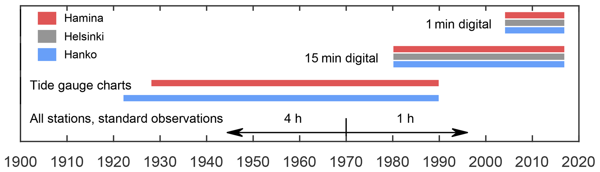
Figure 2Sea level data available from the tide gauges of Hanko, Helsinki, and Hamina in the Gulf of Finland. Only selected events have been manually digitised from the tide gauge charts.
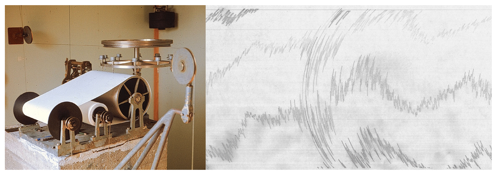
Figure 3The Renqvist–Witting recording device used at most Finnish tide gauges from the 1920s to the early 1990s and an example of the paper charts recorded by the device at Hanko, showing a meteotsunami event on 9–10 May 1969.
High-resolution sea level data before the 1980s are available only on the original tide gauge charts, which are currently stored in the archives of the Finnish Meteorological Institute (FMI). From the 1920s to the 1990s, most Finnish tide gauges were equipped with a Renqvist–Witting recording device (Fig. 3). The device recorded the movements of the float swimming in the tide gauge well by transferring the motion to a wheel (circumference 1 m), on which 10 pens of different colours were fastened. As the wheel turned, the pens plotted the motion on a paper roll in real size (scale 1:1) so that each colour corresponds to a certain decimetre of sea level height (Stenij, 1932). The 4-hourly and hourly values in the digital sea level database have been sampled manually from these paper charts.
The principal data set used in this study consists of the original paper charts from the Hanko and Hamina tide gauges from the periods 1922–1989 and 1928–1989, respectively (Fig. 2). The Helsinki tide gauge was the only Finnish tide gauge not equipped with a Renqvist–Witting device. Instead, a Reitz recorder was used. The glass plate used to read sea level values from Reitz paper charts has not been preserved, and the data are arduous to use. In addition, the small scale of variation in Reitz paper charts hinders the recognition of meteotsunamis. For these reasons, paper charts from the Helsinki tide gauge have been excluded from the study. Digital 15 min sea level data from 1980 onwards is used from all three tide gauges. The 15 min data directly captures oscillations longer than 30 min, and 16–30 min waves are aliased to periods shorter than 4 h. For example, a 20 min oscillation shows up as a 60 min oscillation, which is still inside the meteotsunami frequency range. Possible very fast oscillations, with periods of a few minutes, are lost in the 15 min data.
Analysing the charts includes a lot of manual work. To restrict the amount of data, only the ice-free summer months from May to October were considered. Even though the possibility of meteotsunamis occurring in winter cannot be ruled out, such cases are expected to be very rare on the Finnish coast (see Sect. 5 for discussion).
A notable meteotsunami with a height of up to 1.2 m was observed in the western part of the Gulf of Finland and in the Archipelago Sea on 15 May 1924 (Renqvist, 1926). After this event, the Finnish Institute of Marine Research started to collect observations of sudden sea level changes by preparing a specific form for the purpose and distributing it to pilot stations and lighthouses in Finland. Approximately 60 such forms from 1924 to 1938 are stored in the archives of FMI. Among these, 14 forms contain information of possible meteotsunamis in addition to the well-documented case of 15 May 1924. We use these eyewitness observations as an additional source of information on meteotsunami occurrence in the 1920s and 1930s.
2.2 Atmospheric data
We use air pressure observations from coastal stations to confirm the meteorological origin of the possible meteotsunamis discovered in the sea level data. The stations nearest to the tide gauges are Russarö (Hanko), Harmaja (Helsinki), and Rankki (Kotka, about 24 km southwest from Hamina; Fig. 1). Original paper barograms from these stations exist in the archives of FMI and have been used when available. Digital 10 min data are available from 2001–2006 onwards depending on the station and was used to confirm some of the recent events.
To study the connections between meteotsunami occurrence and climatological factors, meteotsunami observations are compared to monthly climatological data and lightning observations. The North Atlantic Oscillation (NAO) indices are obtained from a data set by Cropper et al. (2014), which includes daily NAO indices since 1850. From this data set, we calculated monthly mean values. The NAO index is calculated from the sea level pressure difference between the Azores and Iceland. It describes large-scale atmospheric conditions in the region, controlling the strength and direction of westerlies and storm tracks.
The atmospheric parameters of mean sea level pressure, 10 m wind speed, 2 m temperature and dew point temperature, and convective available potential energy (CAPE) are obtained from reanalysis data. Two different data sets were used: ERA-20C (covering the years 1922–2010) and ERA-Interim (1979–2014), both produced by the European Centre for Medium-Range Weather Forecasts. ERA-20C has a horizontal resolution of around 125 km or 1.125∘ (Poli et al., 2013) whereas in ERA-Interim, it is around 80 km or 0.75∘ (Dee et al., 2011). We have interpolated the ERA-Interim data to match the resolution of ERA-20C so that the grid points are compatible. The reanalysis data were averaged spatially over the Gulf of Finland region (20.25–30.375∘ E, 59.0625–61.3125∘ N). Finally, daily and monthly mean values were calculated.
We also compare the meteotsunami occurrence to lightning observations. From 1887, thunderstorm days in Finland have been observed by humans, and in 1960–1998 they were observed with an automatic flash counter network. From 1998 onwards, in addition to the number of flashes, the location information of the flash has also been obtained via a modern lightning locating system (Mäkelä et al., 2014). In this study, we compared the meteotsunami data set to the yearly number of thunder days (1922–2014) and the yearly number of cloud-to-ground (CG) flashes over the whole continent of Finland (1960–2014). In addition, from 1998–2014, we calculated daily and monthly CG flash numbers in the Gulf of Finland region (20–30∘ E, 58–62∘ N).
2.3 Data quality
The 15 min digital sea level data (1980–2014) are raw data that has not been subject to thorough processing and quality control. However, the data were browsed through visually, and clearly erroneous spikes and shifts were removed before further analysis. Possible problems in the data are documented and relatively easy to trace. In Hanko and Hamina, the 15 min observations were digitised by a human-assisted computer program over the period 1980–1987. When comparing these observations to the data that was digitised from the tide gauge charts for this study, it was noted that some high-frequency oscillations that were recorded by the instruments on the paper charts are not accurately reproduced in the 15 min data during this period. This problem in the quality of the digitisation does not affect the time series after 1987.
On some occasions, sea level variations recorded at the tide gauges have been suppressed due to blockages or damage in the underwater pipe connecting the tide gauge well to the sea. When the pipe is partially blocked, the water level in the well adjusts slowly to sea level changes, and there is a time lag and attenuation in the recorded sea level fluctuations. We refer to this attenuation as damping. In the worst case, damping is so heavy that all sea level variations have been levelled out. Damping particularly hinders the study of high-frequency sea level variations such as meteotsunamis.
To determine the periods when the high-frequency oscillations were damped in the digital 15 min tide gauge records (1980–2014), a spectral analysis was performed. The variance of oscillations with a frequency higher than 0.25 h−1 (period shorter than 4 h) was integrated from the variance density spectra calculated from 7 d time series. The high spatial and temporal variability in the recorded shorter oscillations was evident already from a visual inspection of the high-frequency variance. However, to quantify the results, a value that was exceeded 95 % of the time (i.e. the 5th percentile) was determined from the Hamina tide gauge records, which were the visually least disturbed. This value was found to be 0.016 m2. The same value was then used in the analysis of all tide gauges. The results were not very sensitive to the exact choice of this cut-off value but produced the same main findings regardless.
The time series was then divided into blocks of four consecutive values, thus representing a time period of 4 weeks. If the variance was below the 5th percentile over half of the time, the 4-week period was flagged as a “damped period”. While this definition is somewhat arbitrary, a couple of results are evident: (i) the records from Hanko are clearly damped during 1985–1989, and (ii) none of the three tide gauges have suffered from significant damping since the beginning of the 2000s. The maintenance of the tide gauges was considerably improved when automatically registering devices were installed. Before that time, reacting to problems was slow because the tide gauge charts were collected once a month and it took almost 1 month to read and analyse them.
It was not possible to perform a similar spectral analysis for the data before the 1980s (i.e. the tide gauge charts). However, an experienced person can estimate the degree of damping visually by comparing the behaviour of the sea level curve to normal variations. The degree of damping in the paper charts was roughly estimated as percentages from no damping (0 %) to total damping (100 %) per each month. For the overlapping period 1980–1989 for which there are both digital and chart data available, the two independent methods of estimating the degree of damping (spectral and visual) produced comparable results.
In the tide gauge charts of Hanko (1922–1989), 3.2 % of the data were missing and 17.3 % damped, while in Hamina (1928–1989), 2.0 % of data were missing and 12.4 % damped. Thus, about 20 % of the Hanko tide gauge charts and 14 % of the Hamina charts were either missing or so heavily damped that they were unusable for meteotsunami detection. In the 15 min data from 1990–2014, the proportion of missing or damped data was small: 6 % in Hanko, 0 % in Helsinki, and 1 % in Hamina.
There is no universal definition or criteria for what qualifies as a meteotsunami, as nearly all sea level variations in the tsunami frequency range are of atmospheric origin. In this study, the metrics used for detecting meteotsunamis are the period and height of the sea level oscillations and the occurrence of a rapid change in air pressure simultaneously with the sea level event. For the tide gauge charts, possible cases were selected visually and digitised manually. High-frequency events in the 15 min data were detected with an algorithm that resulted in a manageable amount of possible events to be confirmed or rejected through a visual inspection of air pressure data. A detailed description of the procedures is given in the sections below.
The periods of meteotsunami waves are in the tsunami frequency range spanning from a few minutes to a few hours (Monserrat et al., 2006). The heights of the events were determined from high-pass filtered time series because slower variations influence the water level also during the meteotsunamis. The filter removed the information below a cut-off frequency of 0.25 h−1 in Fourier space and was implemented using the Fast Fourier Transform (FFT).
For each potential meteotsunami event identified in the data, we defined three different height metrics after high-pass filtering the sea level data.
-
hmax. The height (top to bottom) of the largest individual wave.
-
htot. The total range of sea level variation during the event.
-
ηmax. The rise above zero in the filtered signal.
3.1 Detecting meteotsunamis in tide gauge charts
Rapid sea level variations appear as dense oscillations on the Renqvist–Witting tide gauge charts and are easy to locate by visual inspection (see Fig. 3, for an example). To find all possible meteotsunami events, we carried out a three-phase inspection.
-
The tide gauge charts were browsed visually. Exceptionally rapid sea level changes were selected for further inspection and photographed. Loose criteria were applied at this stage in order not to miss any potential meteotsunamis.
-
From the cases selected in the visual browsing, we digitised those where the sea level behaviour clearly differs from surrounding variations. The digitisation was carried out manually with a glass plate designed for reading values from tide gauge charts. The timescale printed on the plate has markings every 1 h, meaning that times between the full hours needed to be estimated.
-
From the digitised cases, we excluded those that were too slow (period longer than 2–3 h) or too small (hmax<12 cm in Hanko and <20 cm in Hamina).
The criterion for wave height was set as follows. First, we determined hmax. Second, we plotted a histogram of all events at the tide gauge in question (not shown) and set the height threshold at the peak of the distribution. It was assumed that the frequency of occurrence should decrease towards higher values and that the peak in the distribution was an artefact resulting from some of the smaller events being included in the visual browsing and some of them being omitted. Therefore, the peak represents the wave height that is clearly visually distinguishable from other sea level variations.
The height criterion applied was different for each tide gauge, because there is large spatial variability in the high-frequency part of the sea level spectrum depending on the location and structure of the tide gauge. In particular, the height of a meteotsunami depends on the bathymetry of the coastal waters and varies strongly from point to point on the coastline. The highest oscillations are observed in bays and inlets whose resonant properties amplify the arriving wave (Monserrat et al., 2006).
Finally, the atmospheric origin of the sea level oscillations was confirmed by examining barograms from nearby coastal stations. The events were interpreted as meteotsunamis if there was evidence of a rapid change in air pressure within a few hours of the sea level oscillations – usually a small, sudden jump or drop that stands out from normal variations based on visual inspection. A small proportion of the events were excluded because there was no indication of air pressure changes. The pressure changes accompanying meteotsunamis are small (typically only 1–3 hPa, Monserrat et al., 2006; Pellikka et al., 2014) and not always easy to distinguish, especially if the quality of the air pressure curve is poor. Therefore, and because of missing air pressure data, a notable portion of the potential meteotsunami events was left unconfirmed.
3.2 Detecting meteotsunamis in digital sea level data
Potential meteotsunami events were searched automatically from the 15 min sea level data (1980–2014) of all three tide gauges. It is possible to detect rapid variations in the tsunami frequency range even in 15 min data, but the heights of the events will be somewhat underestimated because of the temporal resolution. First, we calculated the heights of all individual waves (hmax) from the high-pass filtered time series, using the differences of adjacent data points to locate wave tops and bottoms (where the derivative of the signal changes sign). From this wave height data set we picked the waves that exceed the height threshold determined in the tide gauge chart analysis: 12 cm for Hanko and 20 cm for Hamina. For Helsinki, no charts were analysed, so we applied a threshold of 10 cm. The spectra of the filtered 15 min data from Helsinki and Hanko are rather similar, while in Hamina there is clearly more variability in the sea level signal in the tsunami frequency range (standard deviations of the filtered signal are 4.5 mm for Hanko, 4.1 mm for Helsinki, and 9.2 mm for Hamina). To remove multiple occurrences of the same event in the data set, we selected the events that have a time difference of at least 12 h.
As with the chart events, we examined the air pressure data and categorised the events as confirmed, not confirmed, or uncertain depending on whether there was evidence of rapid changes in air pressure. Two examples of the detected meteotsunamis are given in Fig. 4. The first one was digitised from the Hanko tide gauge charts (the original chart is shown in Fig. 3). The second was detected from the 15 min sea level data from Hamina. Both cases have been confirmed from air pressure data.
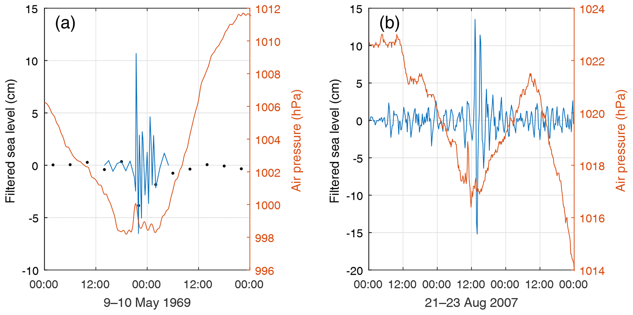
Figure 4(a) A meteotsunami in Hanko on 9–10 May 1969, visually identified and digitised from the tide gauge charts. Black dots show the standard 4 h sea level observations. Air pressure observations from Hanko Russarö, digitised from a paper barogram, are plotted in red. (b) A meteotsunami in Hamina on 22 August 2007, automatically detected from the high-pass filtered 15 min sea level data. Air pressure observations from Kotka Rankki are plotted in red.
4.1 Meteotsunami occurrence in the Gulf of Finland
For Hanko and Hamina, the methods described above result in two time series of meteotsunamis: one based on original tide gauge charts (1922/1928–1989) and the other on 15 min sea level data (1980–2014). A small number of events (4 from Hanko and 6 from Hamina) were excluded from the data set because there was no evidence of rapid changes in air pressure during the event despite air pressure data being available.
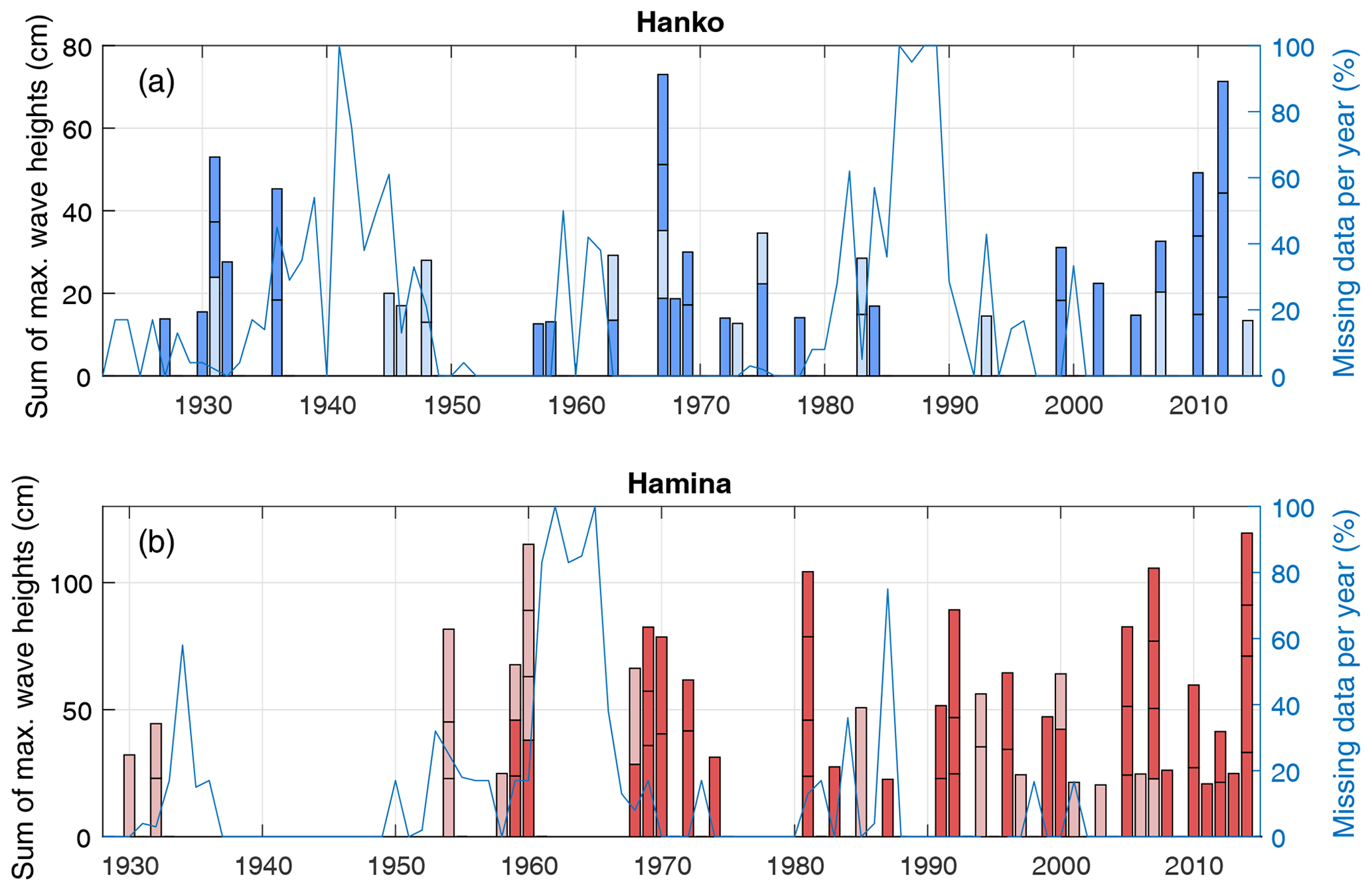
Figure 5Meteotsunamis identified in the sea level data from the 1920s to 2014 for (a) Hanko and (b) Hamina. The events of each year are stacked so that the height of the column corresponds to the sum of maximum wave heights of the events during a given year. Dark-coloured events have been confirmed from air pressure data; the light-coloured events are potential meteotsunamis whose atmospheric origin is uncertain. The blue curves show the proportion of missing or damped data per year.
As there is a 10-year overlap (1980–1989) in the time series, we can compare the performance of the different methods of identifying meteotsunamis in the data. For Hamina, the results are nearly identical: both the visual viewing and the automatic detection identify seven events over the decade, of which six are given by both methods. For Hanko, data from the 1980s is largely missing (Fig. 5) and there are only three possible events found in the tide gauge charts, of which one is detected in the 15 min data. The other two are not properly recorded in the 15 min observations because of quality problems in the digitised data (see Sect. 2.3). Because of these problems, we use the results from the tide gauge charts in the final data set for the 1980s. Nevertheless, the good agreement between the two data sets in Hamina indicates that both the visual viewing and the automatic detection of rapid variations are effective methods of identifying meteotsunamis in the data and the results can be combined with reasonable confidence.
The detection algorithm successfully identifies the known meteotsunami events from the Gulf of Finland on 29 July 2010 and on 8 August 2010 (Pellikka et al., 2014). The event on 15 May 1924 reported by Renqvist (1926) is also detected from the Hanko tide gauge charts, but the maximum wave height is only 8.3 cm, falling below the height threshold. This highlights the limitations imposed by the sparse observation network: even during strong meteotsunami events, when eyewitnesses have observed exceptional sea level oscillations over a large area (exceeding 1 m in some places), the wave heights observed at the tide gauges can be small (Renqvist, 1926; Pellikka et al., 2014).
Only one of the events detected from the tide gauge charts (24 May 1926 in Hanko) was mentioned in old eyewitness reports collected by the Finnish Institute of Marine Research (Sect. 2.1). According to the report from the lighthouse of Seivästö (currently in Pionerskoye, Russia), in the easternmost part of the Gulf of Finland, sea level oscillations of ca. 40 cm occurred within a few minutes in the morning after a nightly thunderstorm. Rapid oscillations were recorded at the Hanko tide gauge during the night, but their height did not exceed the threshold and this event is thus not included in the final data set.
Table 1Number of potential and confirmed meteotsunami events identified in the different data sets. The first column shows the number of events found on the tide gauge charts based on visual inspection. The second column gives the size of the final data set, which are events exceeding a station-specific height threshold ht. Confirmed events have a rapid change in air pressure occurring simultaneously with the sea level oscillations. The rest could not be confirmed because of missing or inconclusive air pressure data.
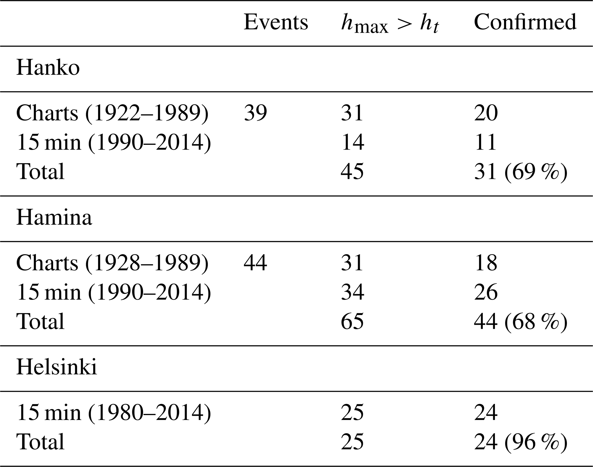
The number of detected events in the different data sets is given in Table 1. In total, 45 potential meteotsunamis were detected from Hanko (1922–2014) and 65 from Hamina (1928–2014). In addition, 25 events were detected in the 15 min observations from Helsinki (1980–2014). When we take into account that 14 of the events were detected at more than one station, we get a total number of 121 separate events. Over 70 % of the events were confirmed from air pressure observations: typically, there is an abrupt change of 1–3 hPa occurring simultaneously with the sea level oscillations or shortly before. The remaining events were left unconfirmed because air pressure data of sufficiently high resolution is not available.
Figure 5 shows all detected and potential meteotsunamis together with the amount of missing data per year. Missing data includes also the data which is so heavily damped that rapid variations in sea level have not been recorded correctly. Detecting trends in the time series is hampered by gaps in the high-frequency data, most notably in the 1940s and 1980s in Hanko and in the 1960s in Hamina.
While the time series from Hanko shows no apparent trend, meteotsunamis in Hamina seem to be more common over the latter half of the century than over the first half. Excluding the years with over 80 % of missing data, the slope of a least-squares fit for Hamina is 4.4 times larger than for Hanko. The positive slope at Hamina is also statistically significant at a level of (at least) p=0.01, while the weaker positive slope at Hanko is statistically significant only at p=0.15.
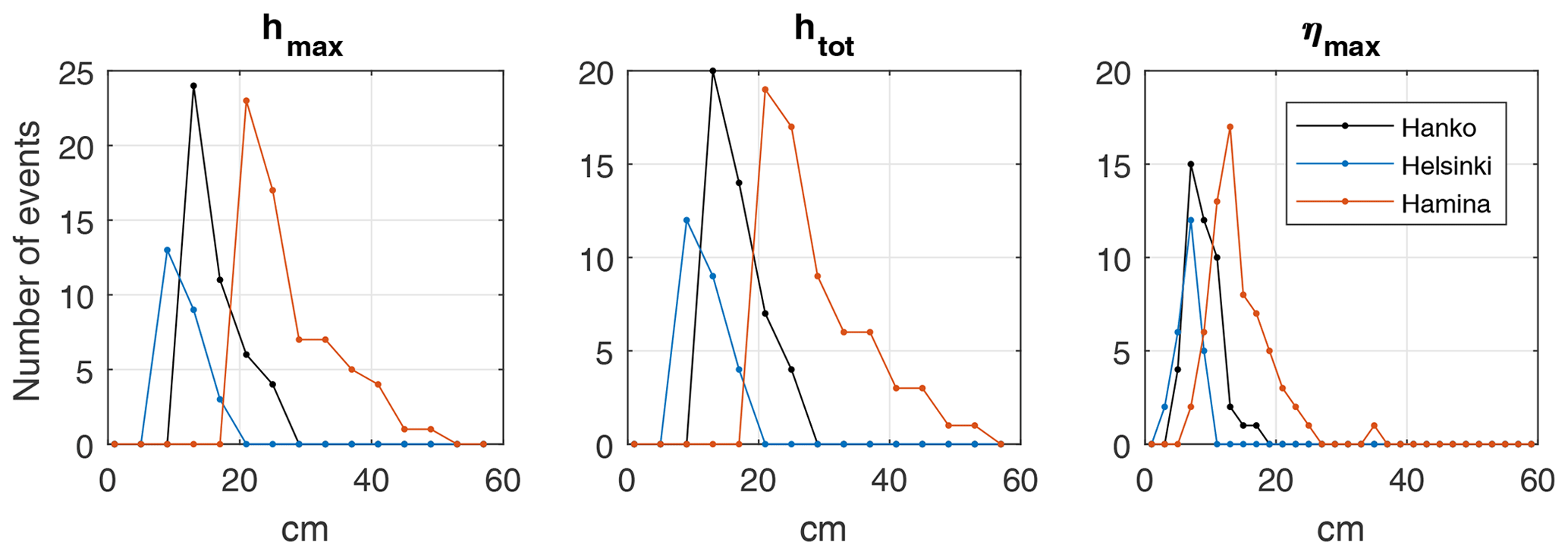
Figure 6Histograms of meteotsunami heights, including both confirmed and potential events from all three stations: the maximum height of a single wave hmax, the total range of variation htot, and the maximum elevation ηmax.
Typical heights of the detected meteotsunamis (hmax) range between 10–30 cm (Fig. 6). The largest meteotsunami heights were found in Hamina, where the highest event was 51 cm (hmax), and the smallest were in Helsinki, where the highest event was 17 cm. The maximum variations during the events (htot) are only slightly higher than the height of the maximum single wave. The maximum water level elevation above zero during the event (ηmax) is typically roughly half of the height of the maximum variation. This indicates that the high-frequency variations during the meteotsunamis are usually quite symmetrical with respect to the still water level determined by the slower changes (that have here been filtered out). There is no statistically significant linear trend for the magnitude of the meteotsunamis (hmax).
4.2 Comparison with atmospheric data
To study the connections between meteotsunami occurrence and the meteorological conditions, we calculated the number of meteotsunamis occurring during each summer month (May–October) from 1922 to 2014. Of the 558 months over this time period, 91 months (16 %) have at least one potential meteotsunami occurrence. The number of events in different calendar months is as follows: 26 events in May, 20 in June, 37 in July, 18 in August, 10 in September, and 10 in October.
We then calculated the mean values of certain atmospheric parameters in the two sets of months: those that have at least one meteotsunami occurrence and those that have none (Table 2). The null hypothesis that the means of these two sets are equal was tested with the two-sample t test, using Satterthwaite's approximation in order not to assume equal variances. The main conclusions remain unchanged even if the potential (uncertain) meteotsunamis are excluded from the data set.
Table 2Means of certain atmospheric variables on the years, months, or days when there is at least one meteotsunami occurrence and when there are none. The statistical significance of the difference is shown at 5 % level. CG flash is cloud-to-ground flash, MSLP is mean sea level pressure, T2 m is temperature at 2 m, D2 m is dew point temperature (at 2 m), U10 m is wind speed at 10 m, CAPE is the convective available potential energy, NAO is the North Atlantic Oscillation, and GoF is Gulf of Finland.
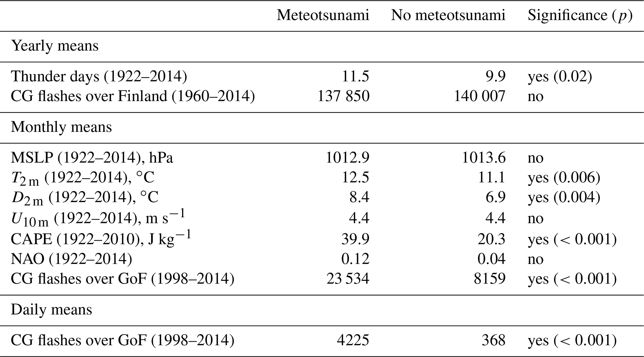
Statistically highly significant (p<0.001) differences were found in the number of CG flashes in the Gulf of Finland area as well as CAPE, which is a measure of convective instability in the atmosphere and often used as an indicator of thunderstorm potential. The mean values of both the temperature and dew point temperature also show a statistically significant (p<0.01) difference, the temperatures being higher during months when meteotsunamis have been registered. Mean sea level pressure, wind speed, and the NAO index did not show a statistically significant difference.
Similarly, we divided the years 1922–2014 in two categories – with meteotsunamis and with no meteotsunamis – and tested the difference in the yearly number of thunder days over Finland. The difference was significant at 5 % level but not at 1 % level. However, there was no significant difference in the number of CG flashes recorded over the whole continent of Finland on a yearly timescale. Finally, the summer days (May–October) over the period May 1998–October 2014 were divided in two categories. The daily number of CG flashes was clearly and statistically significantly (p<0.001) larger during the days of meteotsunami occurrence than during normal conditions.
The lightning observations have a strong connection with meteotsunami occurrence. In the summers of 1998–2014, from which there is daily lightning data available from the Gulf of Finland, there were 42 d on which a potential meteotsunami has occurred in the area. CG flashes have been observed on all of these days except one (30 July 2010), and even on that date, the meteotsunami in Hamina was recorded just after midnight after an active thunder day (5378 CG flashes observed on 29 July 2010). On average, the number of flashes during a meteotsunami day was roughly 10 times that of an average summer day in the region.
We detected 121 potential meteotsunami events at the tide gauges of Hanko, Helsinki, and Hamina in the Gulf of Finland over the past century (1922–2014). Over 70 % of the events were confirmed to coincide with a sudden change in air pressure. Typical wave height registered at the tide gauges was 10–30 cm. However, higher oscillations have probably occurred in bays, harbours, and straits where the coastal bathymetry has amplified the waves. The events detected in the tide gauge data are comparable with the observed meteotsunami events in 2010 and 2011, during which eyewitnesses reported oscillations of up to over 1 m.
Both the number and height of the detected meteotsunamis were largest in Hamina, the easternmost tide gauge. This is probably related to differences in tide gauge locations: disturbances travelling from west to east propagate a longer distance before they hit Hamina compared to Hanko and Helsinki. Moreover, there are differences in local coastal geometry: the tide gauge of Hanko is located on a relatively open coast, while the tide gauge of Hamina is inside a narrow bay that is 5 km long and 1 km wide. In Helsinki, the tide gauge is sheltered by the archipelago but not inside a bay or harbour.
The results are based on 15 min sea level data after 1989, when continuous recordings of sea level variations are no longer available on paper charts. As noted in Sect. 2.1, the 15 min resolution is not ideal for studying meteotsunamis. Oscillations with a period shorter than 30 min are distorted by aliasing, and very short period oscillations cannot be captured. This does not seem to create a significant bias in the results, however. Otherwise, the number of detected meteotsunamis would drop after 1989, which is not the case. Our method also captures the recent meteotsunami events reported by eyewitnesses in 2010 and 2011.
Before the recent eyewitness observations of meteotsunamis in Finland (Pellikka et al., 2014), Finnish sea level researchers did not receive such reports from the general public for at least 30 years. It remains unclear why, as the data show that meteotsunamis occur almost yearly on the Finnish coast and that there is no significant trend in the height of these waves. A lower reporting threshold in the era of the internet and mobile phones is one possible explanation for the upsurge in eyewitness reports. However, data from Hamina give a statistically significant increasing trend in the number of meteotsunamis over the past century. Further research is needed to explain this increase and the fact that no such trend is observed at Hanko. As we note above, the location of the Hamina tide gauge is potentially more vulnerable to meteotsunami amplification. Also, as the height of a meteotsunami is sensitive to the interplay of the arriving wave and coastal bathymetry, it may well be that changes in the propagation direction of atmospheric disturbances result in differing trends at different locations.
There is an identifiable difference between typical heights at the three locations, with Hamina having the largest meteotsunamis and Helsinki having the smallest. However, different degrees of damping due to the blockage of the pipe connecting the tide gauge to the sea were found at all stations. It cannot be conclusively determined to which degree this damping may have affected the amplitude of rapid variations even for data that was not discarded as erroneous. The use of 15 min observations is also expected to introduce a slight negative bias, as the maximum values of 15 min observations are smaller compared to denser data. That said, the finding placing the highest variations in Hamina is expected based on its geographical location furthest in to the Gulf of Finland and inside a small, narrow bay.
Statistically highly significant differences between months when meteotsunamis have been registered compared to normal conditions were found in the number of lightnings over the Gulf of Finland as well as CAPE, which is an indicator of summertime thunderstorm potential. Monthly mean temperatures also show a statistically significant difference. These differences may be partially connected to meteotsunamis being more prevalent during the hottest summer months of June–August and less common in September–October, but the results do demonstrate a strong connection between thunderstorms and meteotsunami occurrence. On a daily level, the cloud-to-ground flash numbers were over 10 times larger during days when meteotsunamis have been registered than otherwise. It can be concluded that meteotsunamis in the Gulf of Finland are practically always connected with thunderstorms.
The study was restricted to summer months (May–October) to keep the amount of data archaeology manageable. Meteotsunamis are expected to be rare in winter, as thunderstorms in Finland are predominantly a summertime phenomenon (Punkka and Bister, 2015). Furthermore, ice cover in the sea reduces the effect of atmospheric disturbances on the sea surface and attenuates especially high-frequency sea level variations. The highest sea levels usually occur in the wintertime on the Finnish coast, and thus meteotsunamis do not generally coincide with annual sea level maxima. This lowers the probability of an extremely high sea level occurring as a combination of a storm surge and a meteotsunami, but quantifying this probability is a topic for future work. Considering coastal safety, an important question is whether meteotsunamis are included in distributions of maximum sea levels. As meteotsunamis are relatively rare, it may be that none have contributed to the monthly maxima, which are often used to estimate coastal flooding risks.
The results show that meteotsunamis as a phenomenon are far more common in the Baltic Sea than previously thought, even though few events are strong enough to be widely noticed or potentially harmful. Many open questions remain regarding Baltic meteotsunamis. An essential topic for future work is to better establish the connections between meteotsunamis and weather patterns. After that, atmospheric parameters could be used to estimate the probability of meteotsunami occurrence and eventually to predict the events. Other suggestions for future research include quantifying potential changes in the propagation direction of atmospheric disturbances and using numerical models to study the resonance phenomena and the effect of local bathymetry on the amplification of the waves.
The data that support the findings of this study are available on request from the corresponding author. Data usage is subject to conditions determined by the data policy of the Finnish Meteorological Institute.
KK and HP designed the study. HP analysed the digital sea level data, and JVB performed the spectral analyses. AK and HB analysed the tide gauge charts, and HP compiled the meteotsunami database. TL calculated the climatological parameters, and HP analysed their connection to meteotsunami occurrence. HP wrote the manuscript with contributions from all coauthors.
The authors declare no competing interests.
We wish to thank the numerous individuals who, over the decades, have worked to maintain the Finnish tide gauge network and sea level database and with their dedication ensured the high quality and preservation of the data. We are grateful to Pentti Pirinen and Achim Drebs for their help with tracking air pressure data from the archives and Simo Siiriä for technical help. We also wish to thank Jadranka Šepić and Milla Johansson for providing valuable ideas and comments. The study has utilised research infrastructure facilities provided by FINMARI (Finnish Marine Research Infrastructure network).
This work was supported financially by VYR (State Nuclear Waste Management Fund) through the SAFIR2014 and SAFIR2018 programs (The Finnish Research Programme on Nuclear Power Plant Safety 2010–2014 and 2015–2018).
This paper was edited by Maria Ana Baptista and reviewed by Agusti Jansa and one anonymous referee.
Bechle, A. J., Kristovich, D. A., and Wu, C. H.: Meteotsunami occurrences and causes in Lake Michigan, J. Geophys. Res.-Oceans, 120, 8422–8438, 2015. a
Cropper, T. E., Hanna, E., Valente, M. A., and Jónsson, T.: A Daily Azores–Iceland North Atlantic Oscillation Index back to 1850, https://doi.org/10.5281/zenodo.9979, 2014. a
Dee, D. P., Uppala, S. M., Simmons, A. J., Berrisford, P., Poli, P., Kobayashi, S., Andrae, U., Balmaseda, M. A., Balsamo, G., Bauer, P., Bechtold, P., Beljaars, A. C. M., van de Berg, L., Bidlot, J., Bormann, N., Delsol, C., Dragani, R., Fuentes, M., Geer, A. J., Haimberger, L., Healy, S. B., Hersbach, H., Hólm, E. V., Isaksen, L., Kållberg, P., Köhler, M., Matricardi, M., McNally, A. P., Monge‐Sanz, B. M., Morcrette, J.-J., Park, B.-K., Peubey, C., de Rosnay, P., Tavolato, C., Thépaut, J.-N., and Vitart, F.: The ERA-Interim reanalysis: Configuration and performance of the data assimilation system, Q. J. Roy. Meteor. Soc., 137, 553–597, 2011. a
Doss, B.: Über ostbaltische Seebären, Gerl. Beitr. Geophys., 8, 367–399, 1906. a, b
Dusek, G., DiVeglio, C., Licate, L., Heilman, L., Kirk, K., Paternostro, C., and Miller, A.: A meteotsunami climatology along the US East Coast, B. Am. Meteorol. Soc., 100, 1329–1345, 2019. a
Jönsson, B., Döös, K., Nycander, J., and Lundberg, P.: Standing waves in the Gulf of Finland and their relationship to the basin-wide Baltic seiches, J. Geophys. Res.-Oceans, 113, C03004, https://doi.org/10.1029/2006JC003862, 2008. a
Leonard, M.: Analysis of tide gauge records from the December 2004 Indian Ocean tsunami, Geophys. Res. Lett., 33, L17602, https://doi.org/10.1029/2006GL026552, 2006. a
Mäkelä, A., Enno, S.-E., and Haapalainen, J.: Nordic Lightning Information System: Thunderstorm climate of Northern Europe for the period 2002–2011, Atmos. Res., 139, 46–61, 2014. a
Masina, M., Archetti, R., Besio, G., and Lamberti, A.: Tsunami taxonomy and detection from recent Mediterranean tide gauge data, Coast. Eng., 127, 145–169, 2017. a
Meissner, O.: Zur Frage nach der Entstehung der Seebären, Annalen der Hydrographie und Maritimen Meteorologie, 52, 14–15, 1924. a
Monserrat, S., Vilibić, I., and Rabinovich, A. B.: Meteotsunamis: atmospherically induced destructive ocean waves in the tsunami frequency band, Nat. Hazards Earth Syst. Sci., 6, 1035–1051, https://doi.org/10.5194/nhess-6-1035-2006, 2006. a, b, c, d, e
Olabarrieta, M., Valle-Levinson, A., Martinez, C. J., Pattiaratchi, C., and Shi, L.: Meteotsunamis in the northeastern Gulf of Mexico and their possible link to El Niño Southern Oscillation, Nat. Hazards, 88, 1325–1346, 2017. a, b
Pattiaratchi, C. and Wijeratne, E.: Observations of meteorological tsunamis along the south-west Australian coast, Nat. Hazards, 74, 281–303, 2014. a
Pattiaratchi, C. B. and Wijeratne, E.: Are meteotsunamis an underrated hazard?, Philos. T. R. Soc. A, 373, 20140377, 2015. a
Pellikka, H., Rauhala, J., Kahma, K. K., Stipa, T., Boman, H., and Kangas, A.: Recent observations of meteotsunamis on the Finnish coast, Nat. Hazards, 74, 197–215, 2014. a, b, c, d, e, f
Poli, P., Hersbach, H., Tan, D. G. H., Dee, D., Thepaut, J.-J., Simmons, A., Peubey, C., Laloyaux, P., Komori, T., Berrisford, P., Dragani, R., Trémolet, Y., Hólm, E. V., Bonavita, M., Isaksen, L., and Fisher, M.: The data assimilation system and initial performance evaluation of the ECMWF pilot reanalysis of the 20th-century assimilating surface observations only (ERA-20C), Shinfield Park, Reading, 2013. a
Punkka, A.-J. and Bister, M.: Mesoscale convective systems and their synoptic-scale environment in Finland, Weather Forecast., 30, 182–196, 2015. a
Renqvist, H.: Ein Seebär in Finnland. Zur Frage Nach der Entstehung der Seebären, Geogr. Ann., 8, 230–236, 1926. a, b, c, d, e
Šepić, J., Vilibić, I., Lafon, A., Macheboeuf, L., and Ivanović, Z.: High-frequency sea level oscillations in the Mediterranean and their connection to synoptic patterns, Prog. Oceanogr., 137, 284–298, 2015. a
Stenij, S. E.: Ein selbstschreibender Apparat für Ausmessung von Mareographenkurven, Societas Scientiarum Fennica: Commentationes physico-mathematicae, VI, 1932. a
Vilibić, I. and Šepić, J.: Destructive meteotsunamis along the eastern Adriatic coast: Overview, Phys. Chem. Earth, 34, 904–917, 2009. a
Vilibić, I. and Šepić, J.: Global mapping of nonseismic sea level oscillations at tsunami timescales, Sci. Rep., 7, 40818, https://doi.org/10.1038/srep40818, 2017. a
Vilibić, I., Monserrat, S., and Rabinovich, A. B.: Meteorological tsunamis on the US East Coast and in other regions of the World Ocean, Nat. Hazards, 74, 1–9, 2014. a