Bias correction of a gauge-based gridded product to improve extreme precipitation analysis in the Yarlung Tsangpo–Brahmaputra River basin

Critical gaps in the amount, quality, consistency, availability, and spatial distribution of rainfall data limit extreme precipitation analysis, and the application of gridded precipitation data is challenging because of their considerable biases. This study corrected Asian Precipitation Highly Resolved Observational Data Integration Towards Evaluation of Water Resources (APHRODITE) estimates in the Yarlung Tsangpo–Brahmaputra River basin (YBRB) using two linear and two nonlinear methods, and their influence on extreme precipitation indices was assessed by cross-validation. Bias correction greatly improved the performance of extreme precipitation analysis. The ability of four methods to correct wet-day frequency and coefficient of variation were substantially different, leading to considerable differences in extreme precipitation indices. Local intensity scaling (LOCI) and quantile–quantile mapping (QM) performed better than linear scaling (LS) and power transformation (PT). This study would provide a reference for using gridded precipitation data in extreme precipitation analysis and selecting a bias-corrected method for rainfall products in data-sparse regions.

1 Introduction

Extreme precipitation often leads to floods, debris flows, and other secondary disasters (Wang et al., 2017), and changes in the frequency and intensity of extreme precipitation profoundly influence both the natural environment and human society (Easterling et al., 2000; Yucel and Onen, 2014). Rainfall observations provide a primary foundation for comprehending their long-term variability and change in extreme precipitation (Alexander, 2016). Accurate rainfall data are necessary for flood protection and water resource management. However, due to scarce spatial coverage of rainfall stations, short-length rainfall records, and high proportions of missing data, observations currently available in some remote basins are clearly inadequate to capture their precipitation characteristics. In addition, observed rainfall data are usually difficult to collect in international river basins because many countries may not share or freely distribute data (Lakshmi et al., 2018).

The Yarlung Tsangpo–Brahmaputra River is the fourth-largest river in the world in terms of flow (Kamal-Heikman et al., 2007) and is influenced profoundly by complex atmospheric dynamics and regional climate processes (Immerzeel et al., 2010; Pervez and Henebry, 2015). Because its agriculture and economy rely heavily on monsoon precipitation, the basin is particularly vulnerable to changing climate (Singh et al., 2016; Liu et al., 2018; Janes et al., 2019; Xu et al., 2019; Zhang et al., 2019). During the four summer monsoon months of June, July, August, and September (JJAS), extreme precipitation with large uncertainties leads to numerous floods (Kamal-Heikman et al., 2007; Dimri et al., 2016; Malik et al., 2016). However, understanding of extreme precipitation in the Yarlung Tsangpo–Brahmaputra River basin (YBRB) has a number of gaps because of its complex topographical interactions with atmospheric flows, lack of observations, and data-sharing issues, which hinder effective flood management (Ray et al., 2015; Prakash et al., 2019).

Currently, different gridded rainfall products provide effective information over regional to global scales, which could be broadly classified into four categories: (1) gauge-based datasets that build on observations from rainfall stations, (2) products from numerical weather predictions or atmospheric models, (3) satellite-only products, and (4) combined satellite–gauge products. The performance of these products varies from region to region (Duan et al., 2016). Given the heterogeneity of orography and climate in the YBRB, observing and modeling its precipitation are very challenging (Khandu et al., 2017). In addition, satellite products are less reliable because high convective rainfall generally takes place in the southern foothills of the Himalayas (Prakash et al., 2015). Compared with some other gauge-based products, the Asian Precipitation Highly Resolved Observational Data Integration Towards Evaluation of Water Resources (APHRODITE) dataset collected more rainfall observations across South Asia (Rana et al., 2015), which have been proven to better estimate spatial precipitation (Andermann et al., 2011). Nonetheless, the lack (and uneven distribution) of rainfall stations at high altitudes in the Tibetan Plateau and Himalayas may introduce uncertainty and affect the accuracy of APHRODITE estimates (Rana et al., 2015; Chaudhary et al., 2017).

Numerous rainfall observations can be obtained from public databases, although their short record and static character limit their direct application in precipitation analysis (Donat et al., 2013). However, these data could be useful for bias correction of gauge-based gridded products by providing additional observations from the denser network of rainfall stations. On the other hand, several methods have been developed to adjust global climate model (GCM) data, ranging from simple linear scaling to more sophisticated nonlinear approaches (Teutschbein and Seibert, 2012). Similarly, these bias-correction methods could be applied to correct gridded rainfall products in sparsely gauged mountainous basins (He et al., 2017). It is important to study whether extreme precipitation analysis could be improved by bias correction of gridded precipitation data and how different methods would influence extreme precipitation indices.

This study evaluated different bias-correction approaches for APHRODITE estimates in the YBRB and assessed their effects on extreme precipitation analysis. We first corrected APHRODITE estimates by both linear and nonlinear methods. Next, we calculated extreme precipitation indices using the original and differently corrected APHRODITE estimates, and the effects of bias correction on extreme precipitation analysis were further investigated by cross-validation. The results provide support to the application of gridded precipitation data and bias-corrected methods in extreme precipitation analysis.

2 Material and methods

2.1 Study area

The YBRB can be divided into three physiographic zones: (1) the Tibetan Plateau (TP), covering 44.4 % of the basin, with elevations above 3500 m; (2) the Himalayan belt (HB), accounting for 28.6 % of the basin, with elevations ranging from 100 to 3500 m; and (3) the floodplains (FP), covering 27.0 % of the basin, with elevations up to 100 m (Immerzeel, 2008).

The moisture in the YBRB is mainly from the Indian Ocean. The YBRB exhibits a broad range of precipitation from the semiarid upstream areas to the HB characterized by abundant orographic rainfall and the vast humid FP. In the upstream areas, precipitation is concentrated during JJAS, and rainfall intensity is mostly low due to long-distance moisture transport (Guan et al., 1984). The irregular topographic variations in the Himalayas profoundly affect the spatial distribution of precipitation by altering monsoonal flow, producing intense orographic rainfall along the Himalayan foothills (Khandu et al., 2017). The downstream areas also receive high rainfall from monsoon flow during JJAS, accounting for 60 %–70 % of the annual rainfall (Gain et al., 2011).

2.2 Data sources

2.2.1 Observational data

In the upper YBRB, rainfall data across China recorded at 31 meteorological stations were collected from the National Meteorological Information Center (NMIC, sourced from the China Meteorological Data Sharing Service System). In addition, data observed at 91 rainfall stations in the downstream area were obtained from the Global Historical Climatology Network (GHCN)-Daily dataset for bias correction. The GHCN-Daily dataset comprises observations from four sources, which have been undergone extensive quality reviews, including the U.S. Collection, the International Collection, the Government Exchange Data, and the Global Summary of the Day. The locations of rainfall stations are shown in Fig. 1.

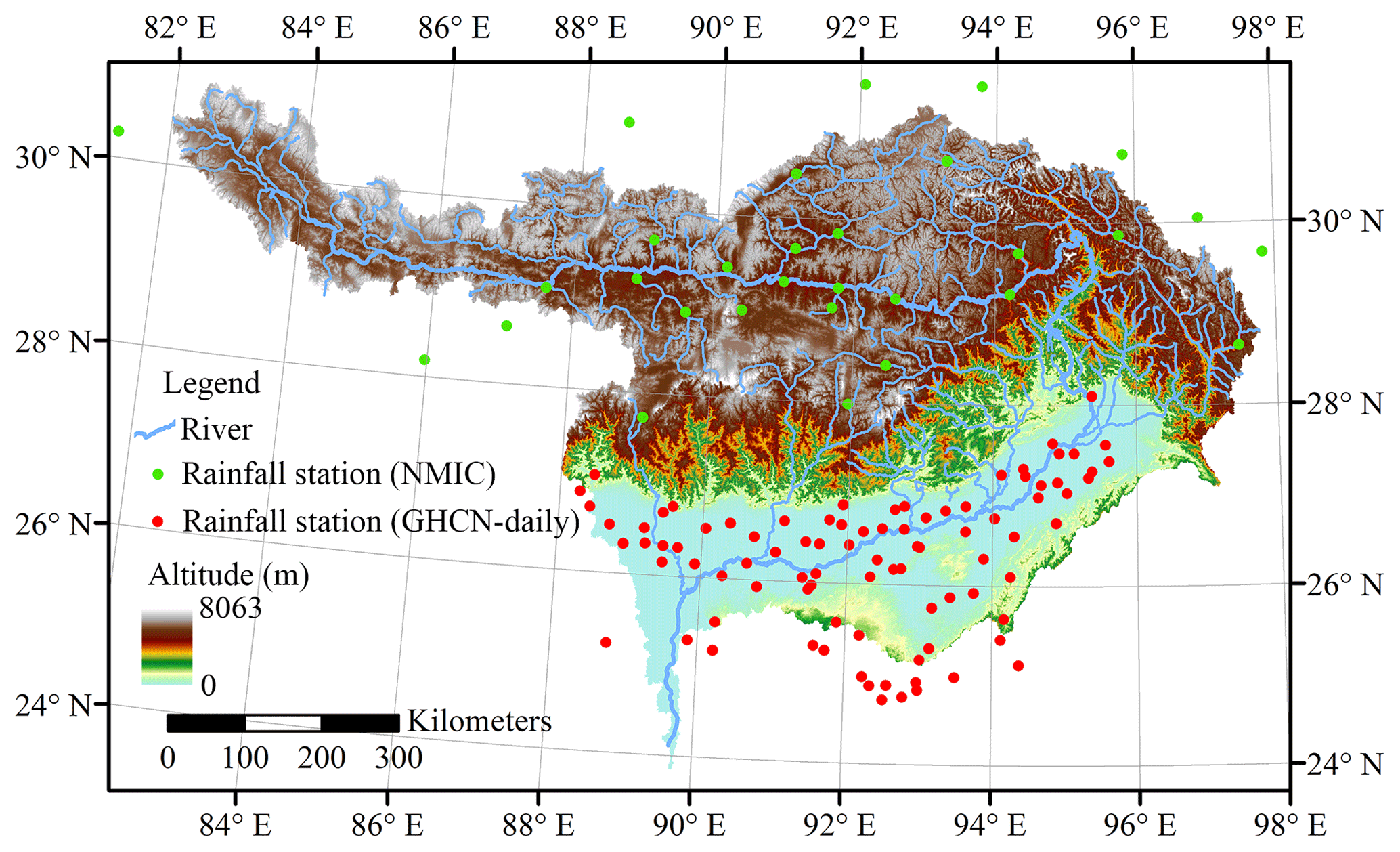
Figure 1 Locations of rainfall stations in the Yarlung Tsangpo–Brahmaputra River basin (YBRB).

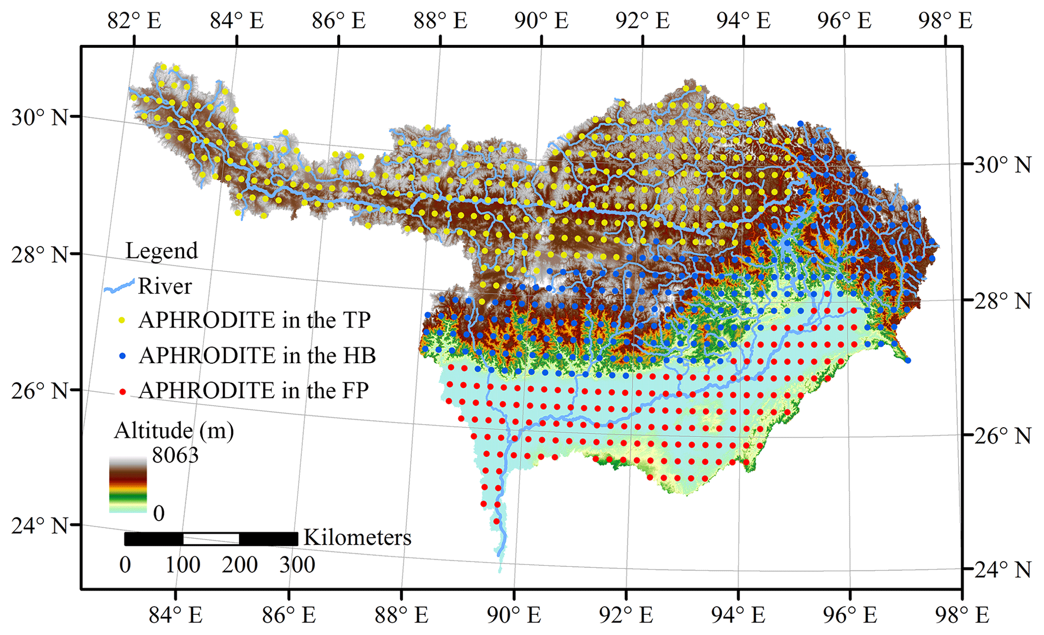
Figure 2 Location of Asian Precipitation Highly Resolved Observational Data Integration Towards Evaluation of Water Resources (APHRODITE) grids over the Tibetan Plateau (TP), Himalayan belt (HB), and floodplains (FP).

2.2.2 APHRODITE estimates

Numerous rainfall observations were incorporated into APHRODITE estimates, including (1) Global Telecommunication System (GTS)-based data, (2) data obtained from other projects or organizations, and (3) their own collection. The rainfall observations that had undergone quality control were gathered, and the ratios of rainfall observations to the world climatology were calculated and then interpolated for each month. The interpolated ratios were multiplied by the world climatology, and the first six components of the fast Fourier transform of the resulting values were used to obtain daily precipitation (Yatagai et al., 2012).

Daily rainfall data of APHRO_MA_025deg_V1101 (http://aphrodite.st.hirosaki-u.ac.jp/index.html, last access: 13 August 2020) at 0.25^∘ resolution in the Asian monsoon area end in 2007, while recently published APHRO_MA_025deg_V1101EX_R1 (http://aphrodite.st.hirosaki-u.ac.jp/index.html, last access: 13 August 2020), using the same algorithm and spatial resolution, extend the time series over the period 2007–2015. Therefore, extreme precipitation could be analyzed from the period 1951–2015 by applying both datasets. To investigate the influence of topography on bias-corrected APHRODITE estimates, the grids were classified into three topographic zones (the TP, HB, and FP; Fig. 2).

2.3 Methods

2.3.1 Bias-correction methods

Two linear methods (linear scaling, LS, and local intensity scaling, LOCI) and two nonlinear methods (power transformation, PT, and quantile–quantile mapping, QM) were used for bias correction in this study.

(1) LS

LS corrects monthly estimates in accordance with observations (Lenderink et al., 2007). It corrects APHRODITE estimates using the ratio between mean monthly observation and corresponding estimation:

$$\begin{array}{}\text{(1)}& P_{\mathrm{APH}}^{*}\left(d\right)=P_{\mathrm{APH}}\left(d\right)\cdot \left[{\displaystyle \frac{{\mathit{\mu }}_{\mathrm{m}}\left(P_{\mathrm{obs}}\left(d\right)\right)}{{\mathit{\mu }}_{\mathrm{m}}\left(P_{\mathrm{APH}}\left(d\right)\right)}}\right],\end{array}$$

where $P_{\mathrm{APH}}^{*}\left(d\right)$ and P_APH(d) are the daily precipitation of the corrected and original APHRODITE estimates, respectively, and P_obs(d) is the daily precipitation observed at the rainfall station in corresponding grid of the APHRODITE estimate. μ_m(P_obs(d)) and μ_m(P_APH(d)) are the mean monthly precipitation of observations and corresponding APHRODITE estimates in the mth month, respectively.

(2) LOCI

LOCI makes a flexible adjustment to the wet-day frequency and intensity (Schmidli et al., 2006; Teutschbein and Seibert, 2012). Firstly, an adjusted precipitation threshold (P_th, APH) is determined so that the number of days exceeding this threshold for APHRODITE estimates matches that of observed days with precipitation larger than 0 mm. Secondly, a linear scaling factor (s) for wet days is computed:

$$\begin{array}{}\text{(2)}& s={\displaystyle \frac{{\mathit{\mu }}_{\mathrm{m}}\left(P_{\mathrm{obs}}\left(d\right)\left|P_{\mathrm{obs}}\left(d\right)>\mathrm{0}\mathrm{mm}\right.\right)}{{\mathit{\mu }}_{\mathrm{m}}\left(P_{\mathrm{APH}}\left(d\right)\left|P_{\mathrm{APH}}\left(d\right)>P_{\mathrm{th},\mathrm{APH}}\right.\right)-P_{\mathrm{th},\mathrm{APH}}}},\end{array}$$

where μ_m(P_obs(d)|P_obs(d)>0 mm) is the mean monthly precipitation of observations with daily precipitation larger than 0 mm and ${\mathit{\mu }}_{\mathrm{m}}\left(P_{\mathrm{APH}}\left(d\right)\left|P_{\mathrm{APH}}\left(d\right)>P_{\mathrm{th},\mathrm{APH}}\right.\right)$ is the mean monthly precipitation of APHRODITE estimates with daily precipitation larger than P_th, APH. Finally, the precipitation data are corrected using

$$\begin{array}{}\text{(3)}& P_{\mathrm{APH}}^{*}\left(d\right)=max\left(s\cdot \left(P_{\mathrm{APH}}\left(d\right)-P_{\mathrm{th},\mathrm{APH}}\right),\mathrm{0}\right).\end{array}$$

(3) PT

PT corrects both the mean and the coefficient of variation in precipitation (Leander and Buishand, 2007), changing precipitation by

$$\begin{array}{}\text{(4)}& P_{\mathrm{APH}}^{*}\left(d\right)=a\cdot {\left(P_{\mathrm{APH}}\left(d\right)\right)}^b,\end{array}$$

where a and b are the parameters of the power transformation, which are obtained using a distribution-free approach and estimated for each month within a 90 d window. Using a root-finding algorithm, the value of b is firstly determined to ensure that the coefficient of variation in the corrected estimates matches that of the observations. The parameter a is then calculated using the mean observation and the corresponding mean of the transformed values.

(4) QM

By shifting occurrence distributions, QM corrects the distribution function of precipitation estimates to match that of observations, which is commonly used in correcting systematic distributional biases (Cannon et al., 2015). A gamma distribution is usually assumed for precipitation events (Teutschbein and Seibert, 2012):

$$\begin{array}{}\text{(5)}& f_{\mathit{\gamma }}\left(\left.x\right|\mathit{\alpha },\mathit{\beta }\right)=x^{\mathit{\alpha }-\mathrm{1}}\cdot {\displaystyle \frac{\mathrm{1}}{{\mathit{\beta }}^{\mathit{\alpha }}\cdot \mathrm{\Gamma }\left(\mathit{\alpha }\right)}}\cdot e^{-\frac{x}{\mathit{\beta }}};x\ge \mathrm{0};\mathit{\alpha },\mathit{\beta }>\mathrm{0},\end{array}$$

where α and β are the shape parameter and scale parameter, respectively.

The cumulative density function (CDF) of the APHRODITE estimates is adjusted to agree with that of the observation, and the daily precipitation for APHRODITE estimates is corrected depending on its quantile. It should be noted that for APHRODITE estimates, many days had low precipitation estimates instead of substantial dry conditions, which may distort the distribution of daily precipitation. Therefore, an adjusted precipitation threshold is also used to ensure the wet-day frequency of corrected APHRODITE estimates match the observed frequency.

$$\begin{array}{}\text{(6)}& \begin{array}{rl}& P_{\mathrm{APH}}^{*}\left(d\right)=\\ & \left\{\begin{array}{l}\mathrm{0},\mathrm{if}{P}_{\mathrm{APH}}\left(d\right)<P_{\mathrm{th},\mathrm{APH}}\\ F_{\mathit{\gamma }}^{-\mathrm{1}}\left(F_{\mathit{\gamma }}\right(P_{\mathrm{APH}}\left(d\right)|{\mathit{\alpha }}_{\text{APH,\hspace{0.17em}m}},{\mathit{\beta }}_{\text{APH,\hspace{0.17em}m}})|{\mathit{\alpha }}_{\mathrm{obs},\mathrm{m}},{\mathit{\beta }}_{\mathrm{obs},\mathrm{m}}),\end{array}\right.\\ & \mathrm{otherwise}\end{array}\end{array}$$

F_γ and $F_{\mathit{\gamma }}^{-\mathrm{1}}$ are the gamma CDF and its inverse, respectively. α_APH, m and β_APH, m are the shape parameter and scale parameter of the original APHRODITE estimates in the mth month, respectively, and α_obs, m and β_obs, m are those of observations in the mth month, respectively.

This study corrected the grids of the APHRODITE estimates that contained time series of observations, and the parameters of bias correction were determined using corresponding available rainfall observations. After that, the APHRODITE estimates from 1951 to 2015 in these grids were corrected by four bias-correction methods. Hereafter, APHRODITE estimates corrected by LS, LOCI, PT, and QM are referred as LS-APHRODITE, LOCI-APHRODITE, PT-APHRODITE, and QM-APHRODITE estimates.

2.3.2 Indices of extreme precipitation

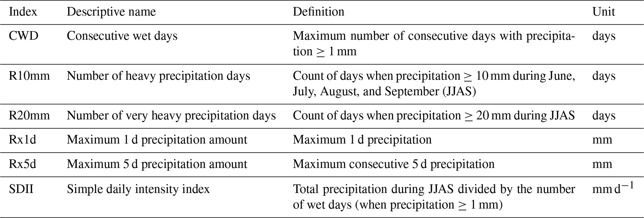
To characterize extreme precipitation during JJAS, six indices recommended by the Expert Team on Climate Change Detection and Indices (ETCCDI), including consecutive wet days (CWD), number of heavy precipitation days (R10mm), number of very heavy precipitation days (R20mm), maximum 1 d precipitation amount (Rx1d), maximum 5 d precipitation amount (Rx5d), and simple daily intensity index (SDII), were applied in this study. Detailed descriptions of these indices are shown in Table 1. The indices fall roughly into three categories: (1) duration indices, which represent the length of the wet spell; (2) threshold indices, which count the days on which a fixed precipitation threshold is exceeded; and (3) absolute indices, which describe the maximum 1 or 5 d precipitation amount (Sillmann et al., 2013).

Table 1 Detailed description of extreme precipitation indices.

Extreme precipitation indices were calculated for corrected APHRODITE estimates in the grids distributed with rainfall stations. To obtain extreme precipitation indices in other grids, inverse distance weighted (IDW) interpolation for extreme precipitation indices were performed. This allowed us to calculate mean values for each of the three topographic zones.

2.3.3 Validation on bias correction

Cross-validation was applied to evaluate the performance of four bias-correction methods. At each rainfall station, the observations were divided into two groups. Two-thirds of the rainfall records were applied to calculate the parameters of LS, LOCI, PT, and QM, respectively. Making use of these parameters, the APHRODITE estimates were then corrected. The mean error (ME) between the extreme precipitation indices obtained from the corrected APHRODITE estimates and those obtained from the remaining third of the rainfall observations were calculated to evaluate the performance of different bias-correction methods.

3 Results

3.1 Evaluation of extreme precipitation indices

The ME of extreme precipitation indices during JJAS for validation are shown in Fig. 3. For the original APHRODITE estimates, the MEs of CWD in the TP, HB, and FP were 8.3, 16.4, and 21.8 d, respectively. There were a lot of days with low precipitation estimations instead of substantial dry conditions, leading to the overestimation of CWD. Likewise, this propagated to LS-APHRODITE estimates with similar MEs of CWD, because there was no change made to the wet-day frequency. The MEs of CWD in the TP, HB, and FP for LOCI-APHRODITE estimates were 3.1, 1.2, and 1.4 d, respectively, and those for QM-APHRODITE estimates were 2.5, 0.8, and 0.9 d, respectively. For both LOCI- and QM-APHRODITE estimates, the days with low precipitation estimations instead of substantial dry conditions were redefined as dry days using the precipitation threshold, resulting in much lower ME and more reliable CWD. Finally, although PT did not directly correct wet-day frequency, the CWD for PT-APHRODITE estimates were lower than those for the original APHRODITE estimates because very low precipitation was corrected.

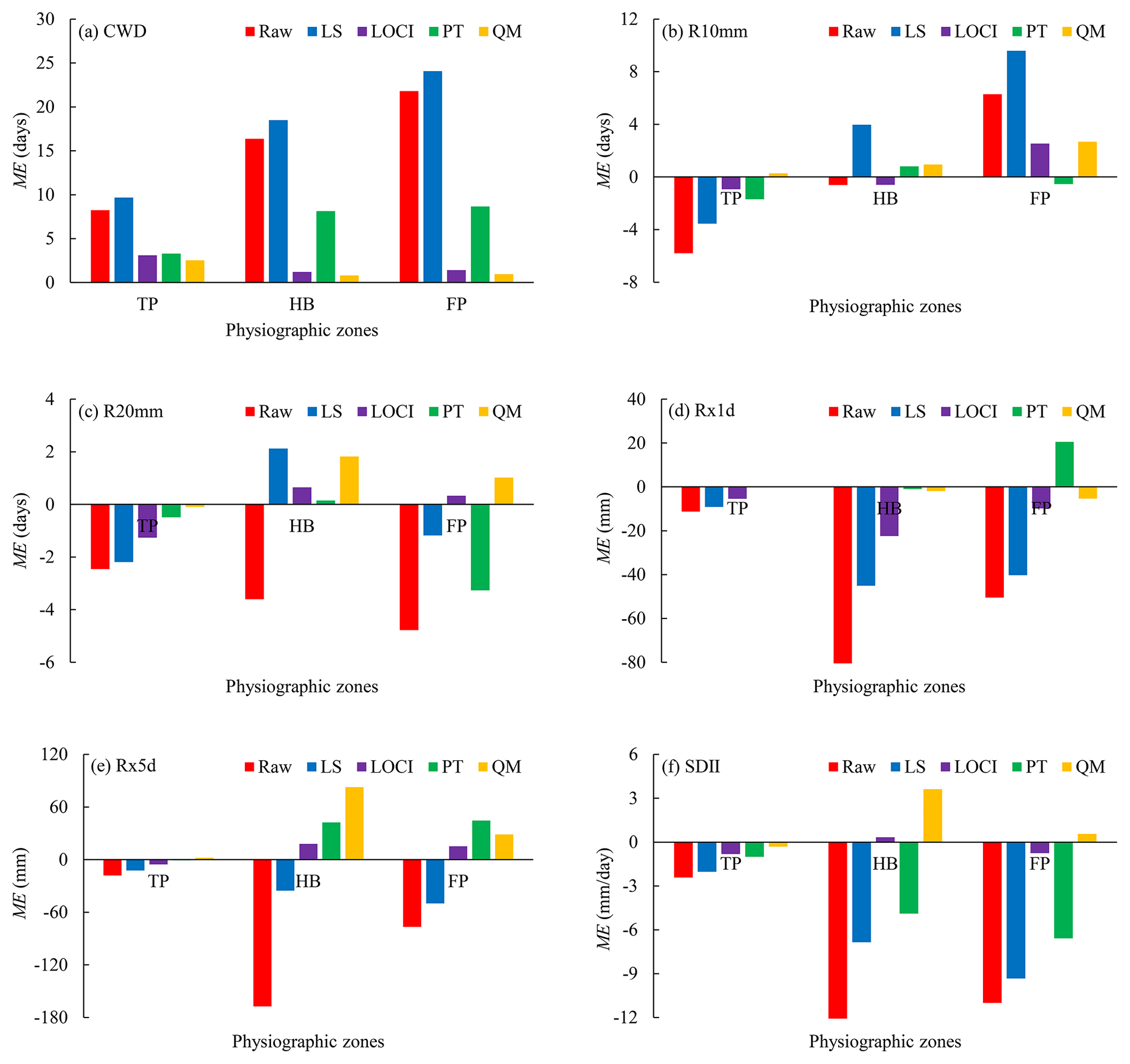
Figure 3 Mean error (ME) of (a) consecutive wet days (CWD), (b) number of heavy precipitation days (R10mm), (c) number of very heavy precipitation days (R20mm), (d) maximum 1 d precipitation amount (Rx1d), (e) maximum 5 d precipitation amount (Rx5d), and (f) simple daily intensity index (SDII) during June, July, August, and September (JJAS) for validation in the three different physiographic zones (TP, HB, and FP) of the YBRB.

The original APHRODITE data tended to underestimate heavy and very heavy precipitation days. Bias correction reduced error in R10mm and R20mm, except for LS, and the absolute values of ME for LOCI-, PT-, and QM-APHRODITE estimates were mostly lower than 1.0 d. LOCI, PT, and QM are able to effectively correct heavy and very heavy precipitation days.

For the original APHRODITE estimates, the MEs of Rx1d were −11.3, −89.1, and −50.5 mm in the TP, HB, and FP, respectively, and those of Rx5d reached −18.0, −167.4, and −76.8 mm, respectively. The original APHRODITE estimates greatly underestimated Rx1d and Rx5d. For the corrected APHRODITE estimates, QM performed best on Rx1d, and the MEs for QM-APHRODITE estimates were −0.1, −1.9, and −5.4 mm, respectively. LS and LOCI used a consistent ratio in linear transformation, resulting in underestimation of Rx1d. In addition, LOCI outperformed other methods for Rx5d, and the overestimation in the HB and FP for PT- and QM-APHRODITE estimates was greater.

The MEs of SDII for the original APHRODITE estimates in the TP, HB, and FP were −2.4, −13.9, and −11.0 mm, respectively. Firstly, heavy and very heavy precipitation in the HB and TP were not fully captured by the original APHRODITE estimates. Secondly, the original APHRODITE estimates overestimated wet days, which distorted the estimation of precipitation intensity. Smaller errors were found in LOCI- and QM-APHRODITE estimates because they corrected rainfall amount and the number of rainy days.

3.2 Extreme precipitation indices calculated from the original and corrected APHRODITE estimates

3.2.1 Extreme precipitation indices in the three physiographic zones

Extreme precipitation indices calculated from the original APHRODITE estimates and four corrected APHRODITE estimates in the three different physiographic zones are shown in Fig. 4. The CWD estimated using the original APHRODITE and LS-APHRODITE estimates were similar. Meanwhile, those derived from LOCI-, PT-, and QM-APHRODITE estimates were much lower.

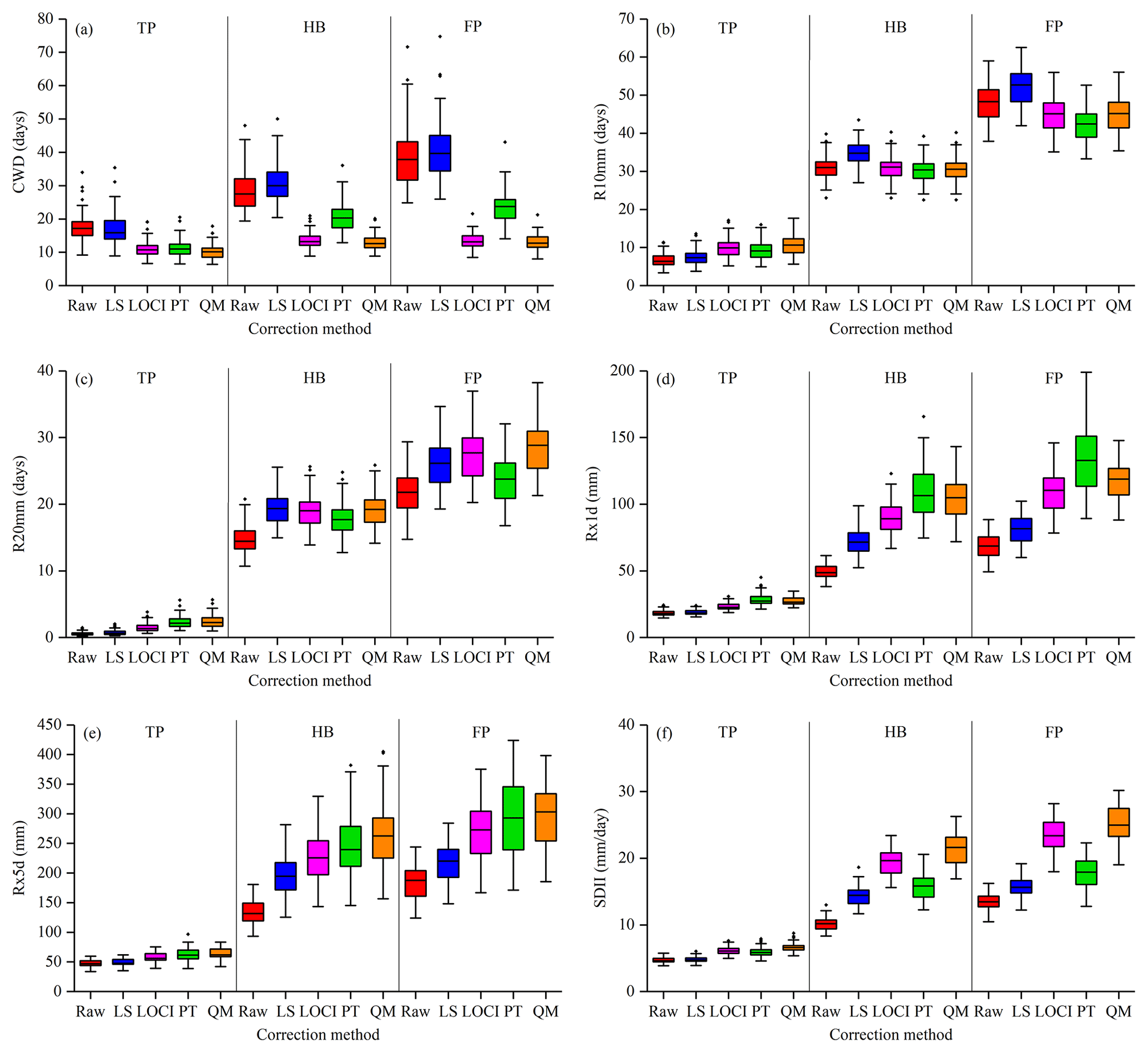
Figure 4 Box and whisker plot for (a) CWD, (b) R10mm, (c) R20mm, (d) Rx1d, (e) Rx5d, and (f) SDII during JJAS in the three different physiographic zones (the TP, HB, and FP) of the YBRB derived from the original and corrected APHRODITE estimates.

Mean R10mm during JJAS obtained by the original APHRODITE estimates in the TP, HB, and FP were 6.7, 31.0, and 47.7 d, respectively. These were similar to those estimated by corrected APHRODITE estimates. However, the differences in R20mm were much more pronounced. Mean R20mm in HB and FP for bias-corrected APHRODITE datasets was close to 19.0 and 26.5 d, respectively, which is approximately 4–5 d higher than those derived from the original APHRODITE estimates.

Compared with the original APHRODITE estimates, the Rx1d and Rx5d increased greatly after bias correction. In the HB, the mean Rx1d obtained from the original APHRODITE estimates was 49.5 mm, while those for LS-, LOCI-, PT-, and QM-APHRODITE estimates were 72.4, 90.1, 109.0, and 103.8 mm, respectively. In addition, the ranges of Rx1d and Rx5d also increased considerably.

The differences in SDII between the original and corrected APHRODITE estimates were also marked. For example, mean SDII in the FP calculated from the original APHRODITE estimates was 13.4 mm. After correction, mean SDII for LOCI- and QM-APHRODITE estimates increased to 23.4 and 25.1 mm, respectively. These values were much greater than those derived from LS- and PT-APHRODITE datasets (15.7 and 17.7 mm).

3.2.2 Relative changes in extreme precipitation indices

The relative changes in extreme precipitation indices during JJAS based on the original and corrected APHRODITE estimates are shown in Fig. 5. The CWD for LOCI-, PT-, and QM-APHRODITE estimates were all lower than the original APHRODITE estimates, yielding relative change rates from −66 % to −27 %. Bias correction decreased the number of rainy days except when using LS. The variations in R10mm and R20mm illustrated that corrected APHRODITE estimates identified much more extreme precipitation events in the TP. The changes in indices varied considerably for different correction methods, with the change rates of R20mm in the TP for LS-, LOCI-, PT-, and QM-APHRODITE estimates being 30.4 %, 169.2 %, 297.1 %, and 317.4 %, respectively. For Rx1d, Rx5d, and SDII, the increases in the HB were much pronounced than those in the FP and TP. Except for the LS-APHRODITE estimates, the increases in Rx1d and Rx5d in the HB were all above 70 % for the corrected APHRODITE estimates.

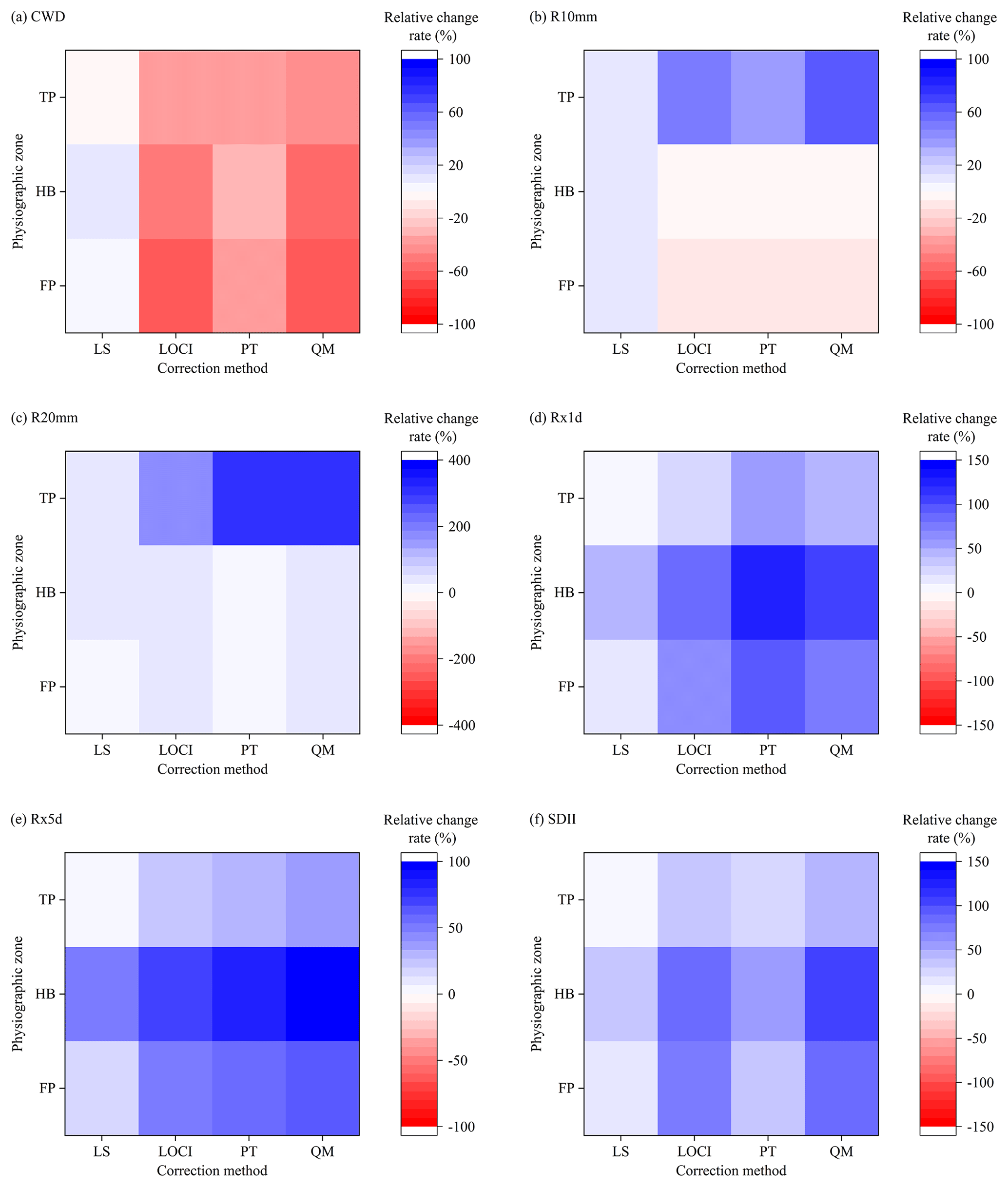
Figure 5 Relative change rate of (a) CWD, (b) R10mm, (c) R20mm, (d) Rx1d, (e) Rx5d, and (f) SDII during JJAS for the original and corrected APHRODITE estimates.

3.3 Influence of bias correction on the spatial distribution of extreme precipitation indices

Rainstorms over the lower YBRB usually have a duration of 2–3 d (Dhar and Nandargi, 2000), and large multiday precipitation events are crucial to the floods in the basin. Hence, the spatial distribution of Rx5d during JJAS based on the original APHRODITE estimates was compared with corrected APHRODITE estimates in Fig. 6. For the original APHRODITE estimates, the area with Rx5d higher than 300 mm only accounted for 2.0 % of the basin, while the proportions for LS-, LOCI-, PT-, and QM-APHRODITE estimates were 10.9 %, 18.7 %, 21.7 %, and 21.3 %, respectively. The most profound difference between the original and corrected APHRODITE estimates occurred over the windward slopes of the Himalayas before the river flows into the Brahmaputra valley. The Rx5d calculated from the original APHRODITE estimates was lower than 300 mm, while much higher Rx5d was obtained after bias correction, yielding maxima of 946.6, 1030.3, 1105.1, and 1396.6 mm for LS-, LOCI-, PT-, and QM-APHRODITE estimates, respectively. The eastern Himalayas, acting as orographic barriers, push the southwest moist air upwards, leading to heavier extreme precipitation over the windward slopes (Singh et al., 2004; Bookhagen and Burbank, 2010; Dimri et al., 2016). However, the original APHRODITE estimates tended to substantially underestimate this extreme precipitation. Besides the aforementioned region, higher Rx5d along the Himalayan front was also found after bias correction. In this case, extreme precipitation calculated from nonlinear approaches was heavier than that derived from linear methods. In general, bias correction is able to consider topographic effects on the spatial distribution of extreme precipitation more comprehensively.

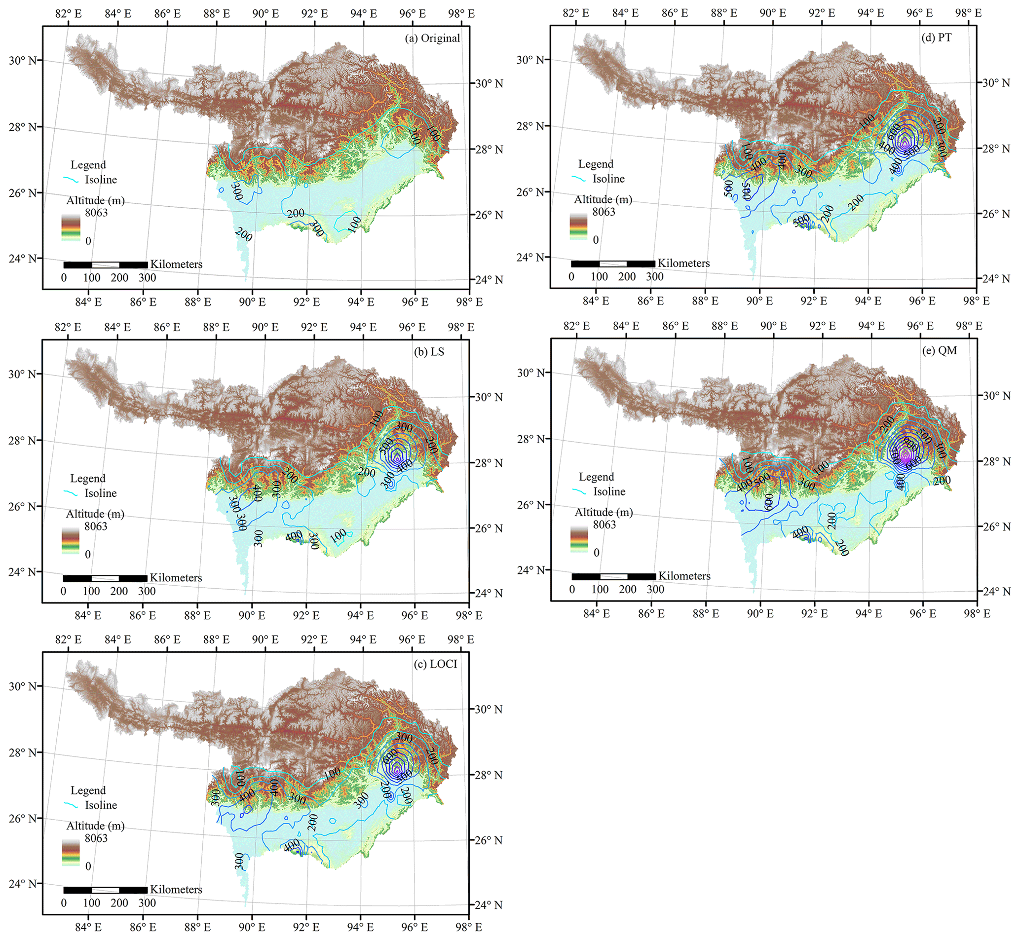
Figure 6 Spatial distribution of mean Rx5d during JJAS in the YBRB based on (a) the original APHRODITE estimates, (b) linear scaling (LS)-APHRODITE estimates, (c) local intensity scaling (LOCI)-APHRODITE estimates, (d) power transformation (PT)-APHRODITE estimates, and (e) quantile–quantile mapping (QM)-APHRODITE estimates.

4 Discussion

Using two linear and two nonlinear bias methods, we corrected APHRODITE estimates during JJAS in the YBRB to investigate the effects of different approaches on extreme precipitation analysis. Extreme precipitation indices were strongly dependent on the bias-correction approach applied.

A primary problem when using gauge-based gridded datasets for extreme precipitation analysis is the fundamental mismatch between point-based observations and gridded estimates (Alexander, 2016). In addition, the spatial coverage of rainfall stations is another major source of uncertainty, particularly where spatial distributions of precipitation are complex (Donat et al., 2013). There are currently several approaches for bias correction, ranging from simple linear scaling to more sophisticated nonlinear methods (Teutschbein and Seibert, 2012). Although mean precipitation corrected by all bias-corrected approaches was similar, the standard deviations and consequent extreme precipitation indices varied considerably. In the case of linear correction, both mean and standard deviation are multiplied by same factor (Leander and Buishand, 2007), resulting in dubious variations in precipitation. Nonlinear correction adjusts the mean and coefficient of variation (Teutschbein and Seibert, 2012), yielding more reliable results. In addition, the typical biases of rainfall products are related to their identification of too many wet days with low-intensity precipitation. Among the four bias-corrected approaches applied herein, LS and PT make no change to the number of rainy days, while LOCI and QM use threshold exceedance to match the wet-day frequency to the observations.

In international river basins, rainfall data are usually not publicly available, and extreme precipitation analysis may suffer from data restrictions (Nishat and Rahman, 2009; Luo et al., 2019). Several great international rivers in South Asia, including the Indus, Ganges, and Yarlung Tsangpo–Brahmaputra, originate from or flow through the Himalayas. Topographic variations in the Himalayas profoundly influence the spatial distribution of precipitation by altering monsoonal flow, resulting in considerable orographic rainfall on the windward slopes (Khandu et al., 2017). Rainfall estimates of different products varied markedly along the Himalayan front and obtained similar results toward the adjacent low-relief domains (Andermann et al., 2011). The GHCN-Daily data can be applied to correct gauge-based gridded datasets in this region, ensuring these products capture the spatial distribution and variation in extreme precipitation. However, numerous GHCN-Daily records in Asia do not contain data from recent years, and the short or incomplete rainfall records limit their direct applications (Donat et al., 2013). Hence, it would be preferable to apply nonpublic datasets in data-sparse regions.

5 Conclusions

Despite increasing use of gridded rainfall products in sparsely gauged river basins, their application in extreme precipitation analysis is challenging due to considerable biases. This study made use of four methods to correct APHRODITE estimates in the YBRB. Their influences on extreme precipitation indices were compared and assessed. The following conclusions were drawn.

1. The original APHRODITE estimates tended to underestimate heavy and very heavy precipitation in the YBRB, and there were a lot of days with low precipitation estimations instead of substantial dry conditions. Bias correction greatly improved the performance of extreme precipitation analysis. The extreme precipitation indices calculated from different corrected APHRODITE estimates varied substantially, and LOCI- and QM-APHRODITE estimates were able to obtain more reliable extreme precipitation indices.

2. Insufficient gauge observations in the Himalayas caused high uncertainty in the heavy precipitation estimates for the original APHRODITE estimates. After bias correction using observations from a denser network of gauges, the heterogeneous orographic effects on extreme precipitation were captured more accurately.