the Creative Commons Attribution 4.0 License.
the Creative Commons Attribution 4.0 License.
 | 29 May 2020
Contrasting seismic risk for Santiago, Chile, from near-field and distant earthquake sources
John R. Elliott
Vitor Silva
Mabé Vilar-Vega
Deborah Kane
More than half of all the people in the world now live in dense urban centres. The rapid expansion of cities, particularly in low-income nations, has enabled the economic and social development of millions of people. However, many of these cities are located near active tectonic faults that have not produced an earthquake in recent memory, raising the risk of losing hard-earned progress through a devastating earthquake. In this paper we explore the possible impact that earthquakes can have on the city of Santiago in Chile from various potential near-field and distant earthquake sources. We use high-resolution stereo satellite imagery and imagery-derived digital elevation models to accurately map the trace of the San Ramón Fault, a recently recognised active fault located along the eastern margins of the city. We use scenario-based seismic-risk analysis to compare and contrast the estimated damage and losses to the city from several potential earthquake sources and one past event, comprising (i) rupture of the San Ramón Fault, (ii) a hypothesised buried shallow fault beneath the centre of the city, (iii) a deep intra-slab fault, and (iv) the 2010 Mw 8.8 Maule earthquake. We find that there is a strong magnitude–distance trade-off in terms of damage and losses to the city, with smaller magnitude earthquakes in the magnitude range of 6–7.5 on more local faults producing 9 to 17 times more damage to the city and estimated fatalities compared to the great magnitude 8+ earthquakes located offshore in the subduction zone. Our calculations for this part of Chile show that unreinforced-masonry structures are the most vulnerable to these types of earthquake shaking. We identify particularly vulnerable districts, such as Ñuñoa, Santiago, and Providencia, where targeted retrofitting campaigns would be most effective at reducing potential economic and human losses. Due to the potency of near-field earthquake sources demonstrated here, our work highlights the importance of also identifying and considering proximal minor active faults for cities in seismic zones globally in addition to the more major and distant large fault zones that are typically focussed on in the assessment of hazard.
- Article
(16490 KB) - Full-text XML
-
Supplement
(12287 KB) - BibTeX
- EndNote


Earthquakes are caused by the sudden release of accumulated tectonic strain that increases in the crust over decades to millennia. Many faults are often not recognised as dangerous because they have not recorded an earthquake in living and written memory (e.g. England and Jackson, 2011). Since probabilistic seismic-hazard assessments (PSHAs) rely on knowledge of past seismicity to determine hazard levels, the regions around these faults are often deemed to be low hazard in seismic-risk assessments until an earthquake strikes and the assessment is revised (Stein et al., 2012). The 2010 Mw 7.0 Haiti earthquake, with its close proximity to an urban centre, was a stark reminder of how ruptures on these faults can be so deadly, especially when they are located near major population centres in poorly prepared low-income nations (Bilham, 2010).
The South American country of Chile is one of the most seismically active countries in the world. Since 1900 there have been 11 great earthquakes in the country with magnitudes 8 or larger (USGS, 2019). All of these were located on or near the subduction interface where the Nazca plate is subducting beneath the South American plate at 7.5 cm yr−1 (DeMets et al., 2010), giving rise to the Andean mountain range (Armijo et al., 2015; Oncken et al., 2006). It is therefore unsurprising that shaking from offshore subduction zone events dominates the seismic hazard – thus the building design – criteria in Chile (e.g. Fischer et al., 2002; Pina et al., 2012; Santos et al., 2012). The most recent great event was the Mw 8.8 Maule earthquake, which struck southern Chile in 2010, generating a tsunami and causing 521 fatalities. However, large, shallow-crustal (<15 km depth) earthquakes are not uncommon in Chile. Since 1900 there have been nine magnitude 7+ shallow-crustal earthquakes located inland and therefore not directly associated with slip on the subduction megathrust (USGS, 2019). But most of these faults accumulate strain at slower rates compared to the subducting plate boundary and thus rupture infrequently.
The San Ramón Fault is one such fault. It runs along the foothills of the San Ramón mountains and bounds the eastern margin of the capital city Santiago, a conurbation which hosts 40 % of the country's population within the city's metropolitan region (7 million according to 2017 estimates). Due to the rapid expansion of the city in the 20th and 21st centuries (Ramón, 1992), parts of the fault now lie beneath the eastern communes (districts) of the city (Fig. 1), in particular Puente Alto, La Florida, Peñalolén, La Reina, and Las Condes. Yet it was only as recent as the past decade that Armijo et al. (2010) recognised that the San Ramón Fault is an active Quaternary thrust fault and poses a significant hazard to the city. Using field mapping and satellite imagery they estimated a slip rate of ∼0.5 mm yr−1 for the fault, a much slower loading rate compared to the overall 7.5 cm yr−1 plate convergence rate in the subduction zone. Palaeo-seismic trench studies across the San Ramón Fault scarp revealed records of two historical ∼5 m slip events – approximately equivalent to a pair of Mw 7.5 earthquakes – 17–19 and ∼8 kyr ago (Vargas et al., 2014). However, based on geophysical investigations of the fault region, Estay et al. (2016) concluded that the San Ramón Fault is segmented into four sub-faults that are most likely activated independently in earthquakes with moment magnitude in the range of 6.2 and 6.7. While Estay et al. (2016) do not discount the possibility of a larger rupture linking across all four segments, evidence from the trench studies (Vargas et al., 2014) suggests that larger-magnitude earthquakes are possible on the fault. Therefore for the seismic hazard and risk analysis in this paper we take the worst-case scenario of a complete rupture along the fault as our scenario case study.
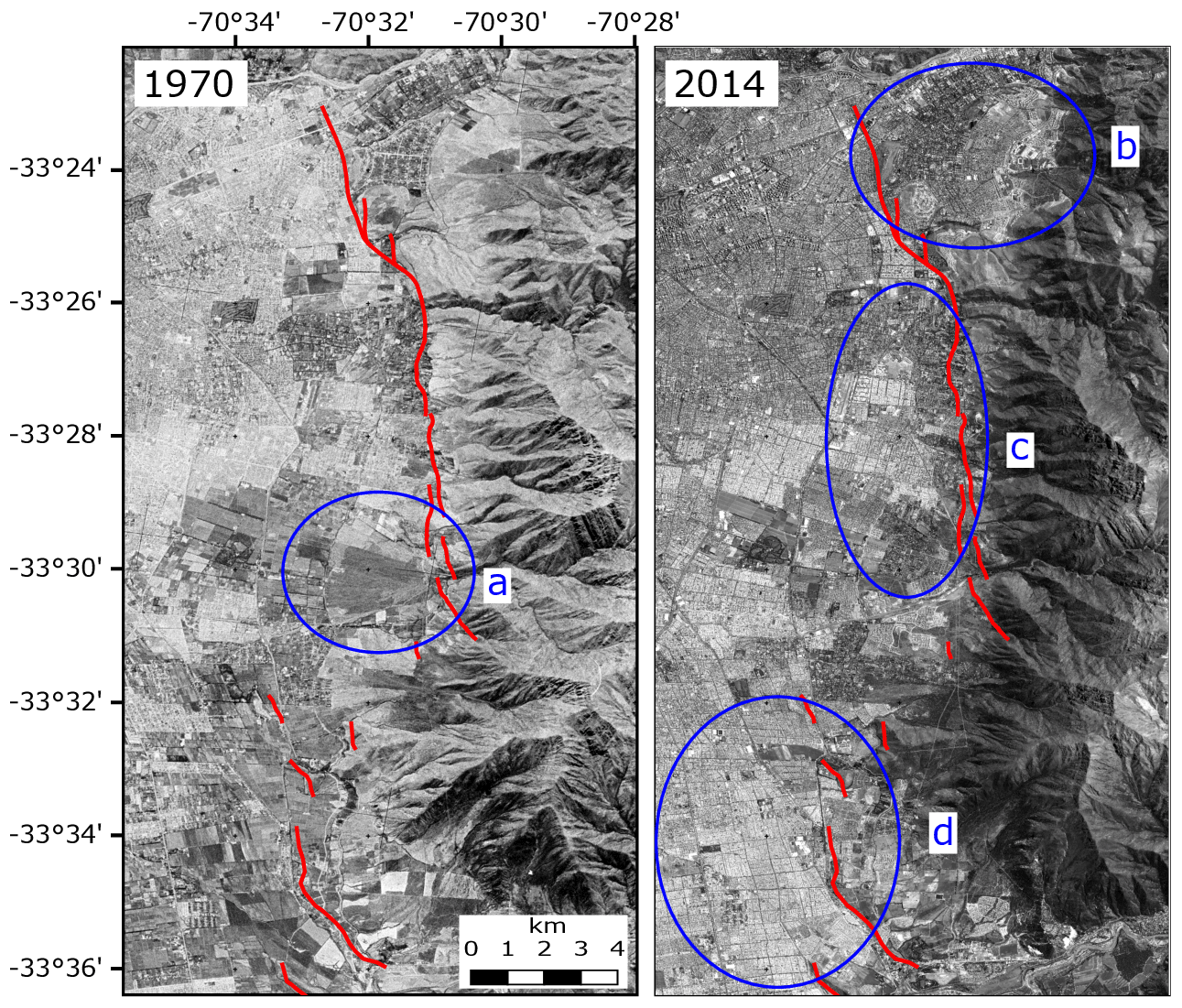
Figure 1Declassified corona satellite image (∼2 m resolution) from 1970 (left) and the same region in the SPOT imagery (1.5 m resolution; right) used in this study showing the eastward expansion of the city over the San Ramón Fault (red lines). Four notable regions are highlighted in blue: (a) an alluvial fan that is clearly visible in the older imagery but completely covered with buildings in the recent image, (b) expansion into the foothills of the mountain and onto the hanging wall of the San Ramón thrust fault (these are often more affluent neighbourhoods with better views across the city), (c) urban densification in the central regions, and (d) land use change from farmland to dense urban neighbourhood masking the fault trace.
Riesner et al. (2017) used balanced kinematic reconstructions of the geology across the region to deduce a long-term average shortening rate of between 0.3 and 0.5 mm yr−1, which is compatible with the earlier estimates by Armijo et al. (2010) and the recurrence slip rates deduced from the palaeo-earthquakes in the trench study by Vargas et al. (2014). This suggests that most of the active deformation across the West Andean fold-and-thrust belt is accommodated on the San Ramón Fault. Therefore, despite the very low slip rates, the long time interval since the last earthquake means that significant strain has now accumulated on the fault, and if it were to rupture completely, it could produce earthquakes of an equivalent magnitude as those recorded in the trench.
Pérez et al. (2014) performed a detailed analysis of local seismicity for the region and showed that the microseismicity at depth (∼10 km) can be associated with the San Ramón Fault, implying that the fault is indeed active and accumulating strain. Vaziri et al. (2012) used Risk Management Solutions' (RMS) commercial catastrophe risk modelling framework to estimate the losses from future earthquakes on the San Ramón Fault for Santiago. They estimate that a Mw 6.8 earthquake on the fault could result in 14 000 fatalities with a building loss ratio of 6.5 %. However, the spatial distribution of these losses remains unclear.
Building on this previous work of identifying the hazard and losses, we aim to contrast the risk posed by the San Ramón Fault and place it in the context of other potential earthquake sources and a previous far-field subduction earthquake (Maule 2010). As we are examining the losses due to a very-near-field source with exposed elements immediately adjacent to the potential rupture, we seek to delineate the location, extent, and segmentation of the San Ramón Fault to improve the accuracy of the ground motion. Stereo satellite optical imagery is often used to derive high-resolution digital elevation models (DEMs) over relatively large areas, which can be useful in identifying subtle active tectonic geomorphic markers of faulting as well as in examining fault segmentation (Elliott et al., 2016). In this paper we use DEMs created from high-resolution satellite imagery from the SPOT and Pléiades satellites (1.5 and 0.5 m resolution respectively) to better characterise the surface expression of the San Ramón Fault and to also look for other potential fault splays within the city limits. Following a similar method as Chaulagain et al. (2016) and Villar-Vega and Silva (2017) and using the Global Earthquake Model's (GEM) OpenQuake Engine (Silva et al., 2014), we explore the contrasting losses to the residential-building stock in the capital through scenario calculations for (a) future earthquakes on the San Ramón Fault, (b) earthquakes on a hypothesised shallow splay buried beneath the centre of the city, (c) deep intra-slab events, and (d) the 2010 Mw 8.8 Maule earthquake. Our models help us to identify particularly vulnerable parts of the city and enable us to make targeted geographical recommendations to improve the seismic resilience of these communities.
We also explore losses to the non-residential-building stock using the Risk Management Solutions (RMS) commercial risk model. The RMS model provides a different view of the commercial risk, where the model is well calibrated due to the availability of losses from previous events and covers the insured assets, which is often one of the main mechanisms to recover from disasters.
Freely available global elevation data from the Shuttle Radar Topography Mission (SRTM) (Farr et al., 2007) have a spatial resolution of 30 m, which is insufficient to accurately map the San Ramón Fault scarp or look for other potential fault splays expressed in the geomorphology. To overcome the low-resolution issue, we analysed SPOT-6 stereo satellite imagery over a 35 km×36 km region covering Santiago city and the San Ramón mountains. The SPOT-6 panchromatic imagery (acquired in 2014) has a spatial resolution of 1.5 m. We also requested the acquisition of very high resolution (0.5 m panchromatic, acquired in 2016) Pléiades tri-stereo imagery over a smaller region (5 km×36 km) covering just the San Ramón Fault (Fig. 2). We performed photogrammetry analysis using commercial software (ERDAS IMAGINE 2015) to produce topographic point clouds from the SPOT and Pléiades stereo imagery. We removed excessive low noise from the point clouds by initially doing a ground classification with only the highest points in a 3.5 m by 3.5 m grid and removing points that were highly isolated in wide and flat neighbourhoods before redoing the ground classification with the filtered points. We then created raster-gridded digital elevation models with 10 and 2 m ground resolutions with the de-noised SPOT and Pléiades point clouds (∼83 and ∼60 million points respectively). We did this by first triangulating the point cloud into a temporary triangular irregular network (TIN) and then rasterising the TIN into a digital elevation model.
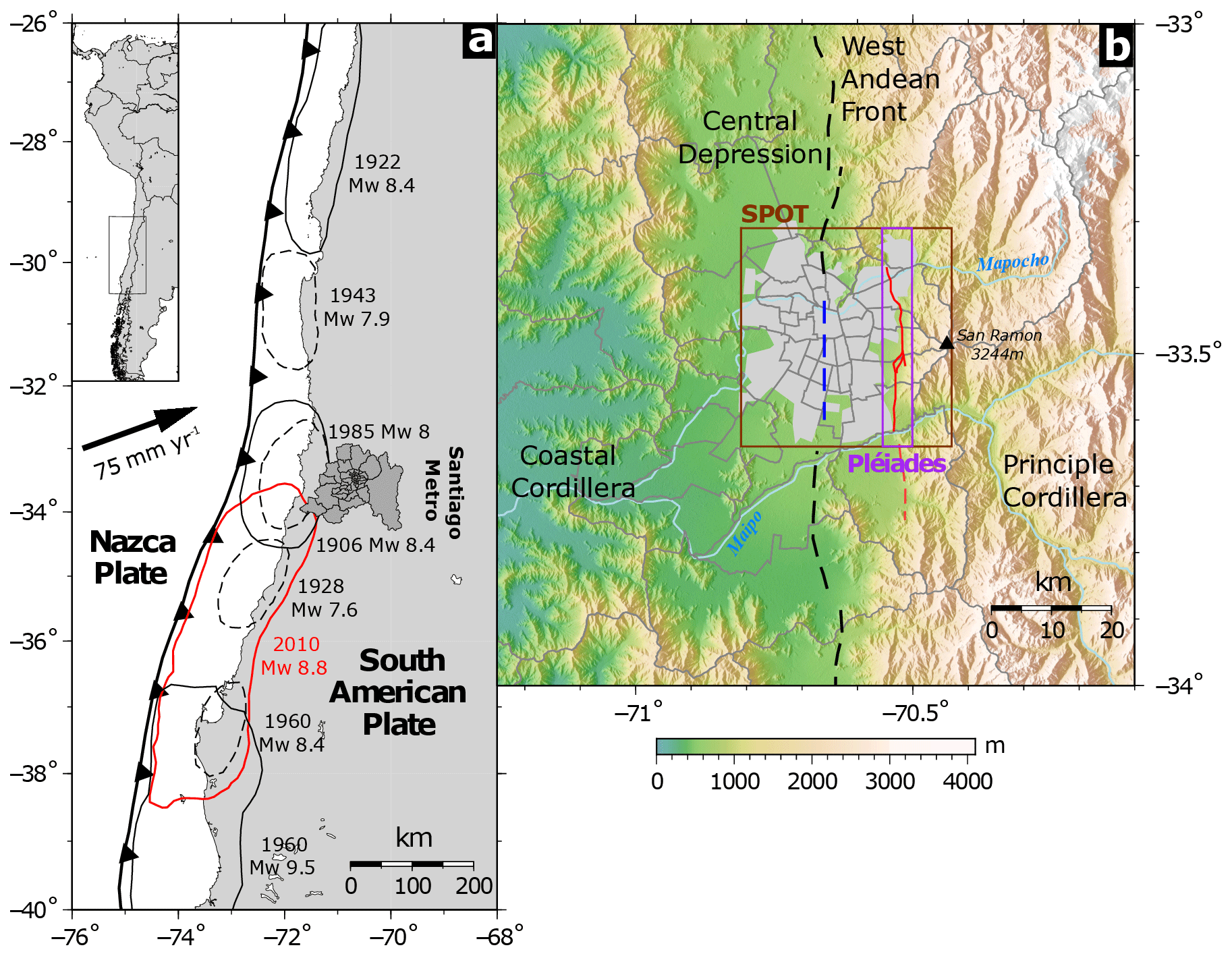
Figure 2(a) Map of central Chile showing the location of great earthquakes for the past century in the subduction zone where the Nazca plate is converging beneath the South American plate at a rate of 43 mm yr−1 (Zheng et al., 2014). The Santiago metropolitan region is shown in the dark grey outline, subdivided by commune (names of all the communes are given in Fig. S1). (b) A 90 m SRTM shaded terrain map of the region around Santiago city (light grey). The SPOT and Pléiades satellite data used in this study cover the region shown by the maroon and purple polygons respectively. The San Ramón Fault is shown in red, while the dotted blue line is the location of our inferred buried fault within the city (see text for details). The dashed black lines are the mountain front faults mapped by Armijo et al. (2010).
The San Ramón Fault is not immediately obvious in the Pléiades elevation map (Fig. 3) beyond the overall morphology of the uplifted San Ramón mountains with a relief of 2.5 km above the Santiago basin. However the fault scarp is clear in the hillshaded DEM, slope and, and terrain ruggedness index (TRI) maps (Fig. 3a, iii–v) as a north–south trending lineament. The terrain ruggedness index is a measure of the local variation in elevation about a central pixel (Riley et al., 1999; Wilson et al., 2007). A TRI of 0 indicates flat terrain while a value of 1 indicates extremely rugged terrain. Such analysis can highlight the change in elevation and slope at a fault scarp. We use these datasets to map the surface expression of the San Ramón Fault, confirming and building on previous work by Armijo et al. (2010), who used a 10 m DEM.
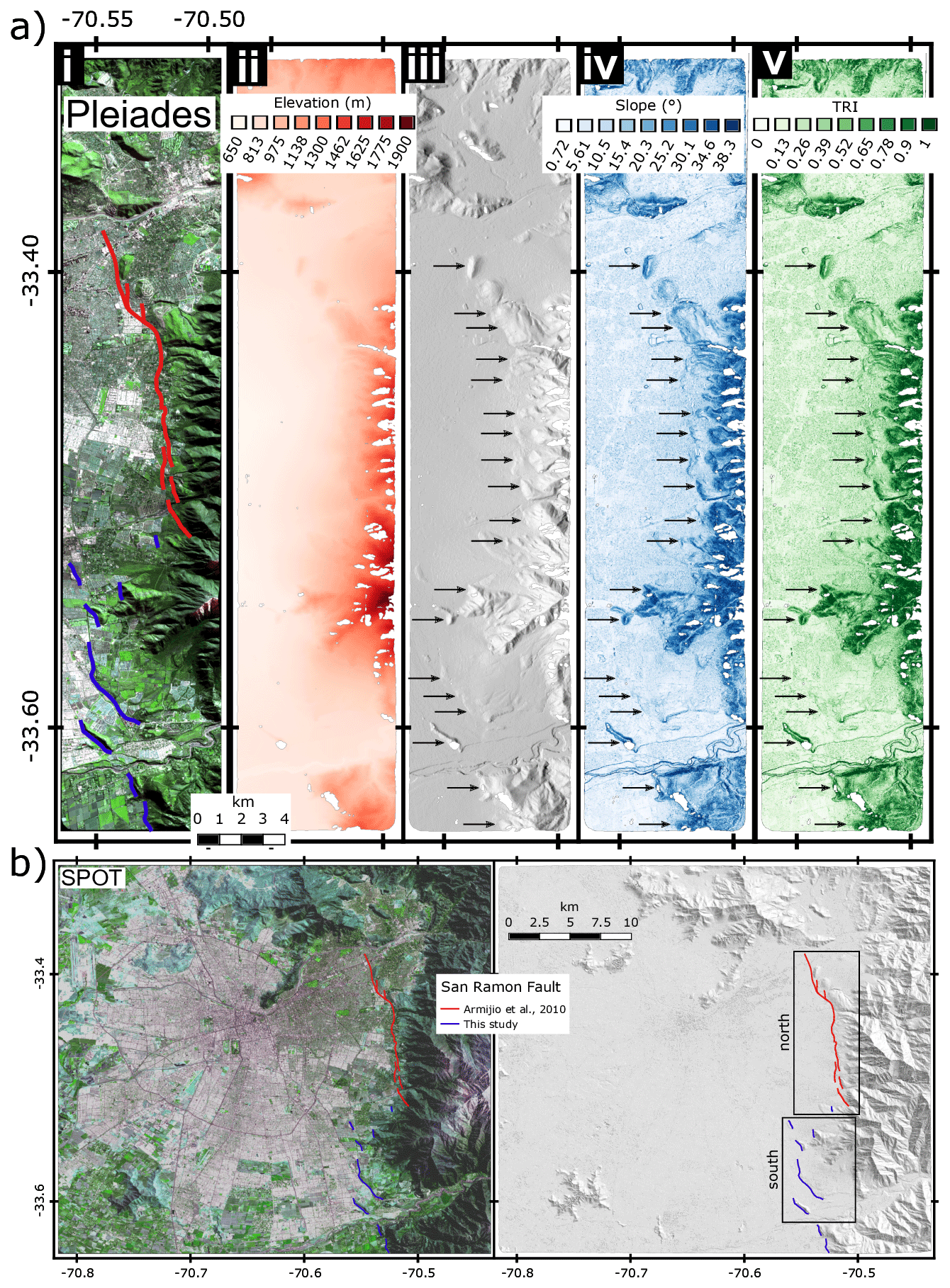
Figure 3(a) (i) The Pléiades satellite optical multispectral image, (ii) the elevation map created using photogrammetry analysis of the panchromatic optical image, (iii) the hillshaded digital elevation model (DEM), (iv) slope map, and (v) – the terrain ruggedness index (TRI). Data gaps are on steep slopes in shadow, resulting in low contrast and inability to derive heights from stereo image matching. (b) The SPOT satellite multispectral image (left) and the resulting hillshaded DEM (right) derived from stereo panchromatic pairs. (Pléiades © CNES, 2016; distribution by Airbus DS/Spot Image.)
The identification of the active fault trace at the surface provides some evidence for the length, location, and segmentation of the fault at depth, and that information is used as a constraint in the subsequent risk analysis for the range of earthquake sources that we seek to test. Measuring the vertical offset across the scarp can give an idea of the past activity along the fault with the caveat that due to natural erosion processes, scarps tend to degrade with time. To do this we plotted a series of west–east profiles across the foothills of the San Ramón mountains to identify and measure the scarp height along the fault by determining the vertical offset between the best fit lines through the point cloud either side of the fault scarp (green and red lines in Figs. 4 and 5). The variable topographic slope along the fault means it is difficult to fit lines of equal length for each profile. In most cases we have tried to ensure a fit through at least 500 m, but where possible 1 km, of points on either side of the fault scarp.
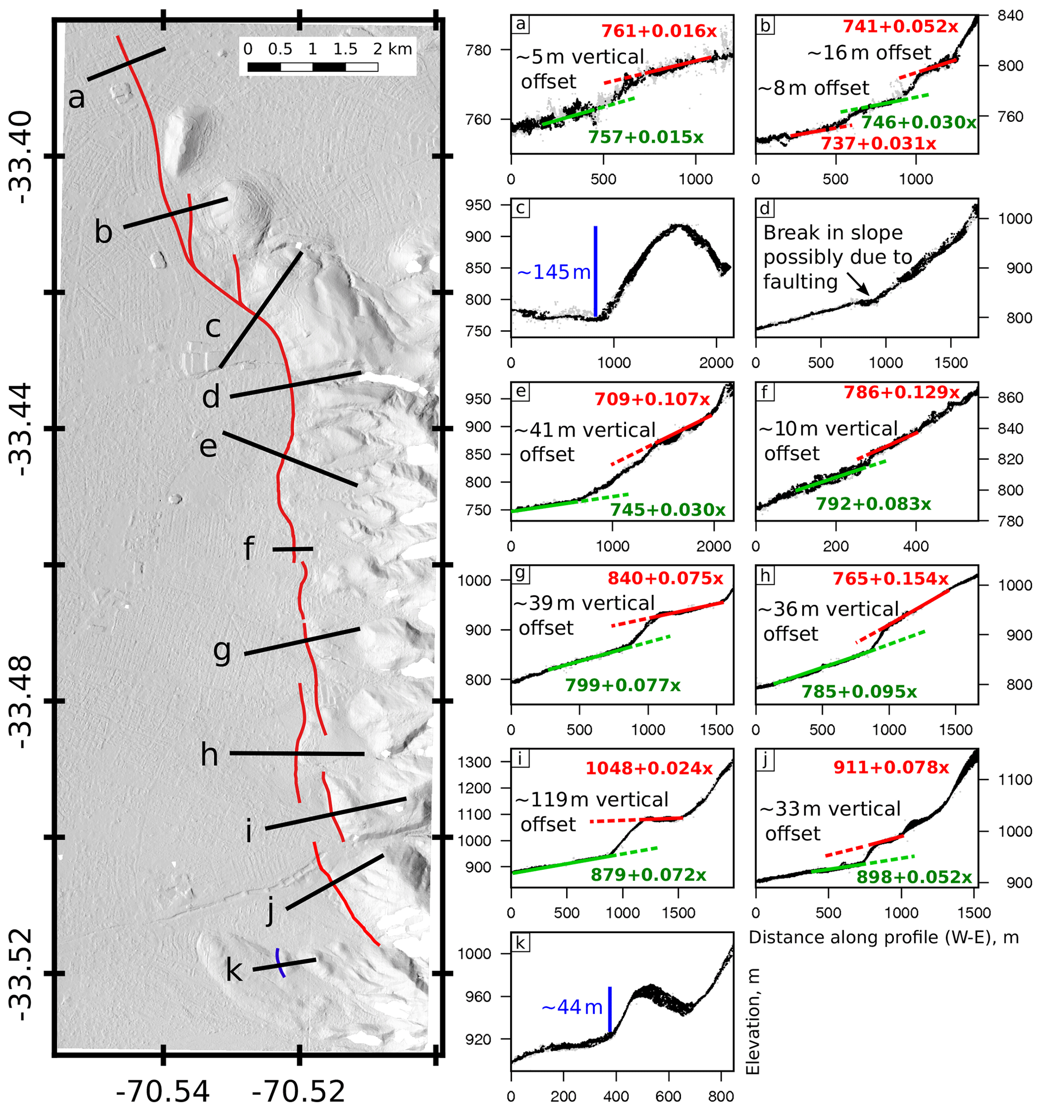
Figure 4The northern section of the Pléiades-derived DEM (2 m resolution) indicated in Fig. 3. The black points on the profiles are ground pixels within a 30 m swath of the profile line from the Pléiades-imagery-derived point cloud, while the grey are from the SPOT point cloud. The red and green lines are best fit lines through the point clouds either side of the fault scarps. The scarp height is estimated from the vertical offset between these two lines. The blue lines are the height of anticlines measured from the downslope side.
In the northern section we found scarp heights to vary between ∼5 and ∼119 m along the fault trace (Fig. 4). Profile d shows no clear evidence of a fault scarp, but since this profile is near a stream channel the scarp is moderated by fluvial erosion. However, it contains a clear break in slope, which is indicative of active faulting. Profiles c and k cross anticlines (∼145 and ∼44 m high respectively) that have likely grown as a result of long-term movements in the hanging wall of the fault. The anticline shown in profile k cuts across the northern section of an alluvial fan, implying its growth post-dates the age of the fan deposit.
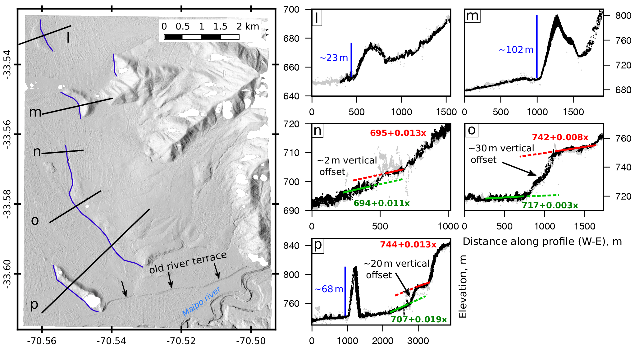
Figure 5The southern section of the Pléiades DEM indicated in Fig. 3. The black points on the profiles are ground pixels from the Pléiades-imagery-derived point cloud, while the grey are from the SPOT point cloud.
In the southern section the scarp heights vary between ∼2 and ∼30 m (Fig. 5). Profiles l and m show two folds with heights of ∼23 and ∼102 m respectively. The growth of the fold in profile p (∼68 m high) shows evidence that it blocked and diverted the Maipo river further south to its current position.
Our estimate of ∼33 m for profile j and ∼39 m for profile g are equivalent to the 31 and 40 m estimated by Armijo et al. (2010). However, our estimate of ∼36 m for profile h is significantly less than their 54–60 m. The range is probably due to our interpretation of the upper slope, which varies due to scarp degradation. This may be because of the relatively lower resolution DEM of 10 m used by Armijo et al. (2010) compared to our 2 m DEM.
Our geomorphic analysis of the surface trace of the San Ramón Fault confirms the findings of Armijo et al. (2010) for the central and northern part of the fault (red line in Fig. 3) and extends the trace of the fault further to the south (blue line in Fig. 3).
In their trench study Vargas et al. (2014) measured fault displacements of the order of ∼5 m. Projected to the vertical for a 45∘ dipping fault, this gives a vertical offset of about 3.5 m. Given that our average measured scarp height is ∼32 m, it is likely that this represents cumulative displacement over numerous earthquakes. However there is significant variation along the fault, with the smallest scarp of 2 m and the largest at 119 m. This variation is probably due to erosion along the mountain front leading to variable degradation of the fault scarps. The smaller scarps represent the cumulative displacements of fewer earthquakes. While these observations enable us to determine the active fault segments that comprise the San Ramón Fault, the variations in scarp height mean it is difficult to trace specific historical ruptures along the fault.
Our observations of the fault traces show a network of fault segments that are ∼0.5 to ∼8 km long. Our assumption is that at depth these segments represent the same fault. This is motivated by field observation that large earthquake ruptures often consist of multiple rupture segments (e.g. Barka et al., 2002; Civico et al., 2018). It is possible that the two main strands of the San Ramón Fault (Figs. 4 and 5) could rupture independently. However, these individual fault segments are not long enough to produce a magnitude 7.5 earthquake from a 5 m slip event, which justifies exploring earthquake scenarios that rupture across both strands of the fault.
The West Andean frontal faults drawn by Armijo et al. (2010) appear to terminate at the northern and southern margins of the city. Although it is possible that the San Ramón Fault accommodates the full shortening across the region, it is also possible that the frontal faults extend further west beneath the city (Fig. 2b), hidden by the sediments of the central depression. Our investigations using the SPOT satellite DEM and point cloud data do not show any clear evidence of a fault scarp within the central regions of the city. However, this could be masked by urban development, or the fault could be buried, as in the case of the Pardisan thrust fault beneath the city of Tehran in Iran, where no primary fault is visible at the surface (Talebian et al., 2016). Similarly, the 2011 Mw 6.3 Christchurch (New Zealand) earthquake occurred on a previously unrecognised fault buried right beneath the centre of the city (Elliott et al., 2012), but its impact was much greater than the larger earthquake (Mw 7.1) that struck the year before outside of the city.
Riesner et al. (2017) proposed a first-order model for the deeper structure of the San Ramón Fault and found that it constitutes the frontal expression of a major west-vergent fold-and-thrust belt that extends laterally for thousands of kilometres along the western flank of the Andes (see also Armijo et al., 2015). Since it is well known that frontal faults of fold-and-thrust belts tend to migrate out of the central highlands through progressive growth of new faulting (e.g. Davis et al., 1983; Dahlen, 1990; Reynolds et al., 2015), it is not unreasonable to assume that younger faults would extend further west from the San Ramón Fault. We project the location of this inferred fault along strike from the West Andean cordillera frontal fault (Fig. 2b) and assume the dip is the same as for the San Ramón Fault. In Sect. 3 we will explore the losses from moderate-magnitude earthquakes (Mw 6 and Mw 6.5) on this hypothesised buried fault within the city with larger magnitude events on the San Ramón Fault (Mw 7 and Mw 7.5), consistent with the palaeo-seismic trench work of Vargas et al. (2014). The magnitudes for the central Santiago splay scenario were determined using standard fault scaling relationships (Wells and Coppersmith, 1994), where a rupture with a length of ∼25 km, a width of ∼12 km, and a co-seismic slip of 1 m would result in an earthquake with moment magnitude in the range of 6–6.5.
In 1647 a large earthquake destroyed Santiago, which at the time was a 100-year-old Spanish town, and killed an estimated one-fifth of its inhabitants (de Ballore, 1913; Udías et al., 2012). Details of this earthquake remain poorly understood, and there is much debate on the epicentral location (e.g. Lomnitz, 1983; Comte et al., 1986; Lomnitz, 2004). Lomnitz (1970) notes that historical descriptions of the damage indicate an epicentre within 50 miles of Santiago at most, while Poirier (2006) mentions that the earthquake did not produce any devastating tsunamis, both pointing to a source on a fault near the city. As there is no evidence of this earthquake in the trench studies along the San Ramón Fault (Vargas et al., 2014), it is unlikely that the earthquake originated there as suggested by Rauld (2002). While it is possible that the earthquake occurred on one of the faults in the principal cordillera (Farías et al., 2010), our assumption was that the main activity in the region is on the frontal portions of the fold-and-thrust belt (e.g. Dahlen, 1990; Reynolds et al., 2015). It is also possible that the 1647 earthquake occurred on the West Andean faults to the north and south of the city (Fig. 2); however, due to the lack of any evidence for either case we feel it is reasonable to explore the worst-case scenario of an earthquake occurring on the extension of these faults through the city.
Another possible candidate for the 1647 earthquake is an earthquake in the subducting slab beneath the city. Therefore, we also examine intra-slab faulting scenarios. This is motivated by the most damaging earthquake in terms of fatalities in south central Chile in the previous century. The 1939 earthquake (Ms∼7.8) caused ∼28 000 deaths (many times more than the great 1960 subduction earthquake) and produced extensive damage to the city of Chillán (Saita, 1940; Frohlich, 2006), about 200 km south of Santiago. Beck et al. (1998) modelled the first P-wave motions for this earthquake and concluded that it was a normal-faulting event within the down-going slab at a depth of 80–100 km. Since the subducting slab beneath Santiago is also about 80 km beneath the city (Hayes et al., 2012), we explore the losses from similar normal-faulting events in the slab beneath Santiago.
The development and implementation of measures to minimise the physical impact due to earthquakes require a comprehensive understanding of the potential for human and economic losses, which is usually achieved through earthquake risk assessment studies (e.g. Silva et al., 2015b; Chaulagain et al., 2016). For risk management purposes, risk is the potential economic, social, and environmental consequences of hazardous events that may occur in a specified period of time (see Grossi and Kunreuther, 2005, for details).
We use the GEM OpenQuake Engine v3.3.2 (Silva et al., 2014; GEM, 2019) to calculate the damage and losses to residential buildings from earthquake scenarios on predetermined faults for all 52 communes that make up the Santiago metropolitan region (∼1.1 million buildings). In the sections below we briefly describe the key components of the damage and risk calculation: exposure, hazard, and vulnerability (Fig. 6).
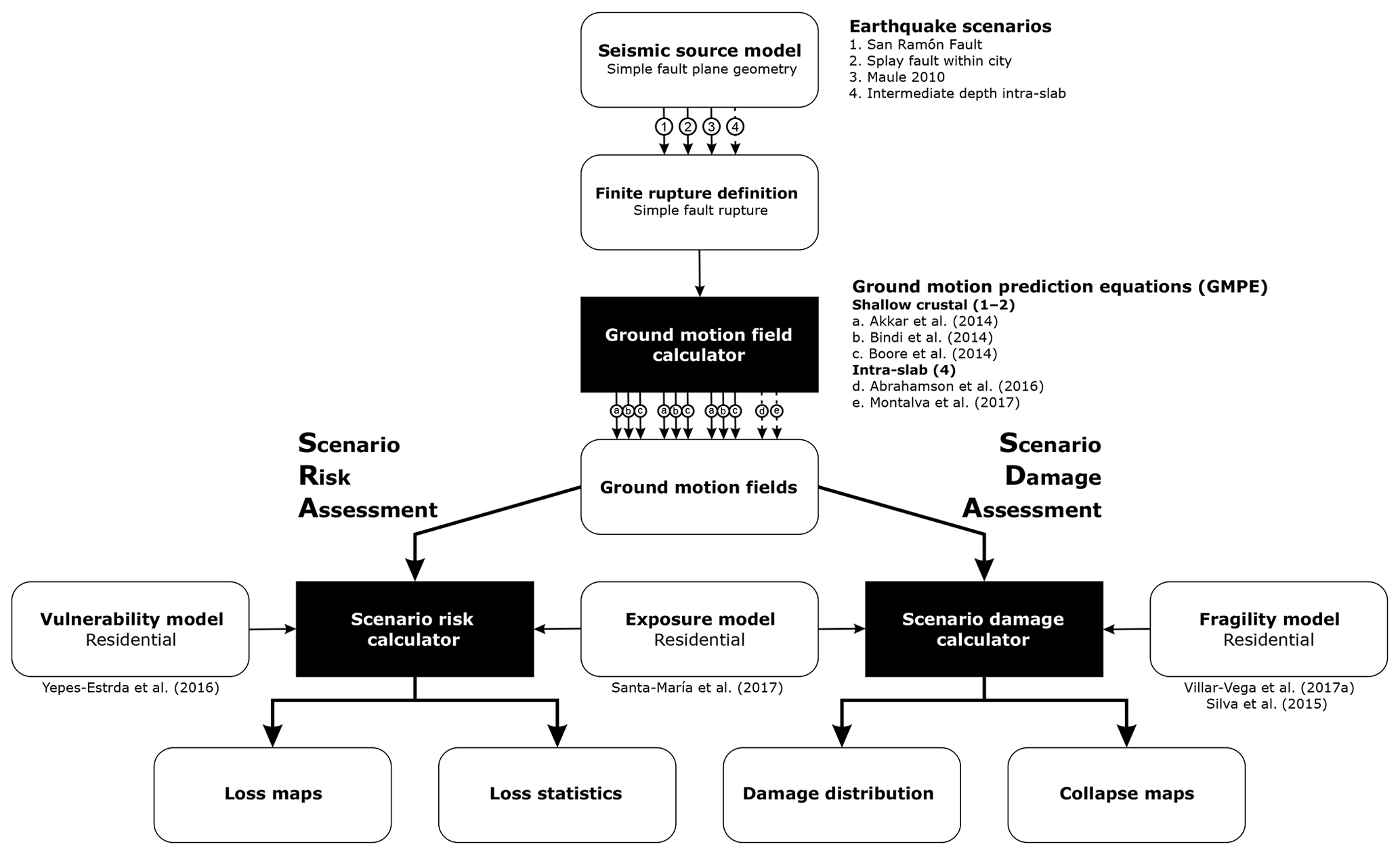
Figure 6A graphical representation of the damage and loss calculation workflow using the Global Earthquake Model's OpenQuake Engine (Silva et al., 2014). Black boxes represent model calculators, while white boxes are data inputs/outputs.
3.1 The residential-building exposure model
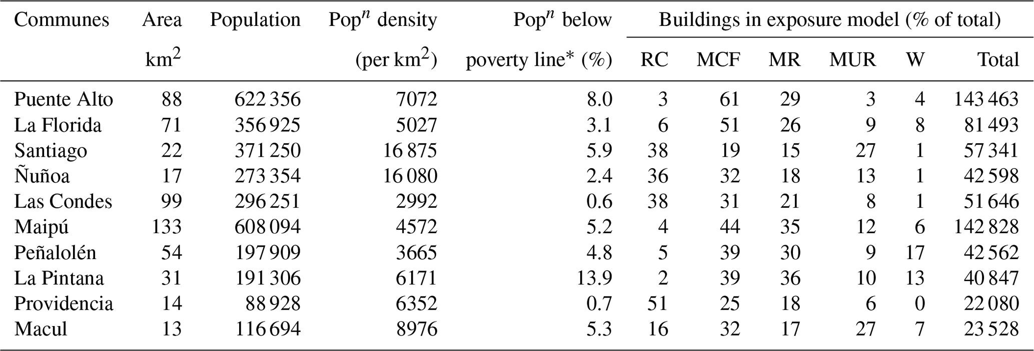
In order to describe the residential-building stock of the Santiago metropolitan region we used the exposure model established by Santa-María et al. (2017). The exposure model was built using data from the national population and housing census surveys (2002 and 2012) and information from the 2002–2014 Formulario Único de Estadísticas de Edificación (Unique Edification Statistic Form; UESF). The exposure model describes the number and distribution of residential buildings at the census block resolution and contains information on the main material of construction, number of storeys (Fig. S2), age of construction, expected ductility, the number of people living in each building, and the replacement cost per unit area. The replacement cost includes an estimate of the structural, non-structural, and content costs of each building. We assume the earthquake scenarios occur at night, and therefore the residential fatality estimates represent the night-time losses. Table 1 summarises the most important information in the residential-building exposure model. The most commonly used building material for residential buildings is masonry (79 % of all buildings), with confined masonry the dominant building typology (39 % of total buildings), followed by reinforced-masonry (26 %) and unreinforced-masonry structures (14 %). To improve computing efficiency we resample the Santa-María et al. (2017) exposure model from the census-block resolution to a 1 km×1 km grid (Fig. S1). Our exposure model reveals that Puente Alto, Maipú, and La Florida are the most populated communes, together accounting for about 26 % of all residential homes in the Santiago metropolitan region. Puente Alto and La Florida are centred on the San Ramón Fault.
Table 1Summary of the building classes and typologies in our Santiago residential-building exposure model, based on Yepes-Estrada et al. (2017).
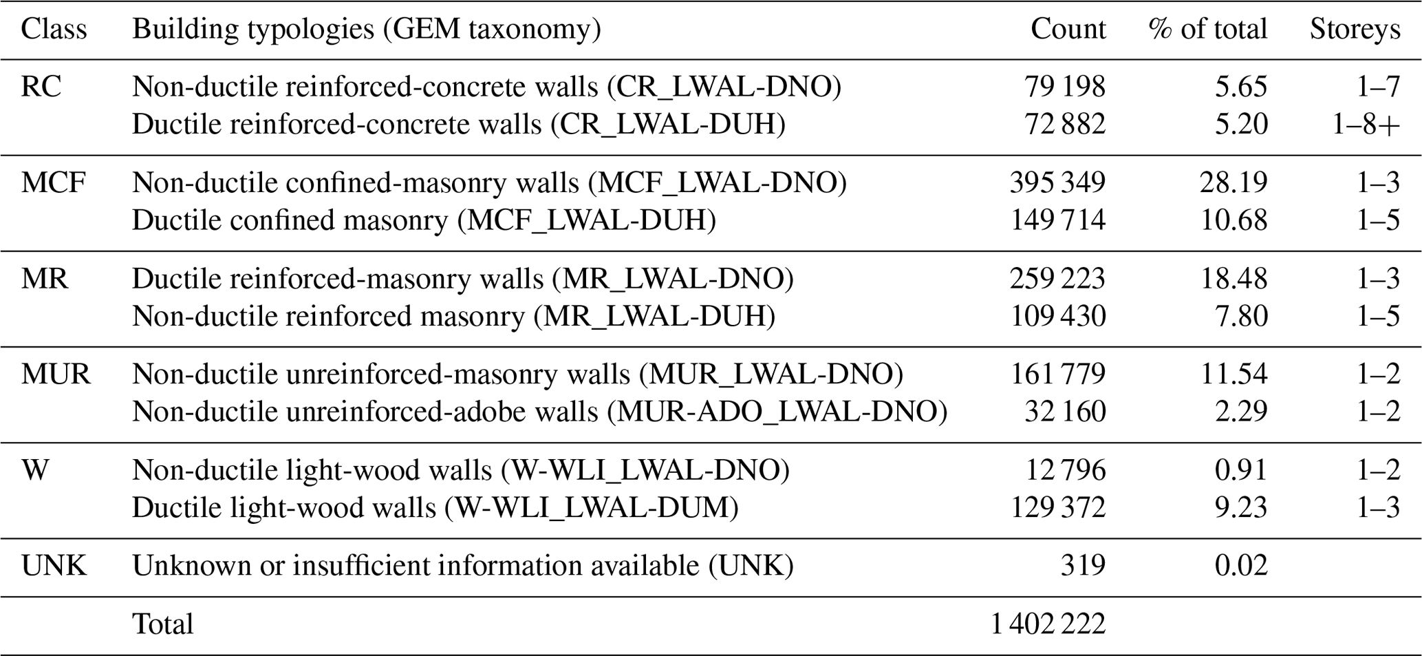
Figure 7 shows the fraction of the total building stock in each commune categorised into the five building classes against the percentage of people living below the poverty line, defined as USD 400 per month for a family of four (Ministerio de Desarrollo Social, 2016). The coefficients of determination (R2) for the fit through each building class are 0.63, 0.01, 0.45, 0.20, and 0.73 for reinforced-concrete (RC), confined-masonry (MCF), reinforced-masonry (MR), unreinforced-masonry (MUR), and wooden (W) buildings respectively. It is clear that the scatter in the data for the masonry buildings is large and reflected in the low R2 values, particularly for MCF buildings, implying little correlation between levels of poverty and the fraction of confined-masonry buildings. However, we find that the fraction of reinforced-concrete buildings decreases significantly with the proportion of people living below the poverty line. This trend is balanced by an increase in the fraction of wooden, reinforced-masonry, and unreinforced-masonry buildings with level of poverty.
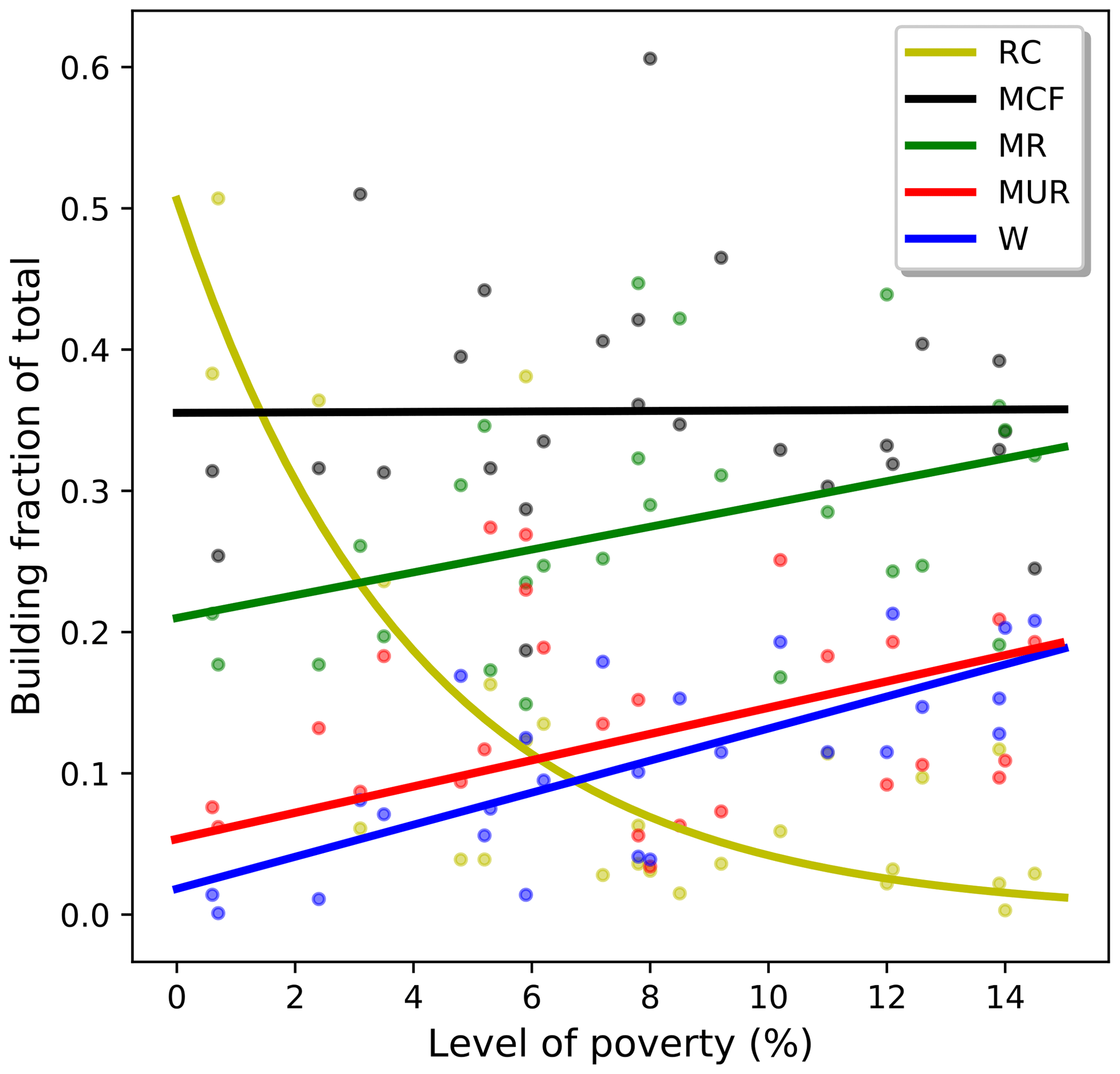
Figure 7The fraction of residential buildings by building class – RC is reinforced concrete, MCF is confined masonry, MR is reinforced masonry, MUR is unreinforced masonry, and W is wooden construction – against the proportion of people living below the poverty line in the communes of the Santiago metropolitan region. Solid lines represent best-fit trends through the data (linear for all cases except for reinforced concrete, which is exponential), with coefficients of determination of 0.63, 0.01, 0.45, 0.20, and 0.73 for RC, MCF, MR, MUR, and W respectively. The poverty line is defined as USD 400 per month for a family of four (Ministerio de Desarrollo Social, 2016).
3.2 Definition of the earthquake scenarios
Unlike probabilistic seismic-hazard analysis where the risk calculation is initiated with a stochastic event dataset, in this study we calculate the damage and losses for specific earthquake scenarios on predetermined faults. We chose a scenario-based approach because it provides clear communication of the relative scale of potential damage and losses from the recently recognised proximal San Ramón Fault versus that from the better-characterised offshore subduction faulting, which is important for emergency management planning and for raising societal awareness of risk (Silva et al., 2014).
We modelled the San Ramón Fault as a set of four rectangular slip planes (total length of 35 km) to account for the changes in geometry along strike due to fault segmentation from our DEM analysis (Fig. S3). The prescribed fault planes dip at 45∘ to the east and extend from the surface down to 12 km depth based on the structural cross sections drawn by Armijo et al. (2010) and the depth of microseismicity determined by Pérez et al. (2014) as indicators of the down-dip width that is locked and accumulating strain. The location of the hypothesised splay fault is in line with the West Andean Front and 12 km west of the San Ramón Fault, consistent with the approximate 10 km spacing inferred in the major thrust faults beneath the San Ramón–Farellones Plateau (Pérez et al., 2014). We represent the splay fault using a single 45∘ eastward-dipping rectangular plane extending from 0.5 km below the surface down to 12 km depth, with a north–south strike running 25 km along longitude 70.65∘ W. The deep intra-slab fault scenario is modelled using a single westward-dipping rectangular plane with a length of 35 km in the subducting slab beneath the city. We used a 70∘ dip for the intra-slab fault to represent a similar earthquake to the 1939 Chillán earthquake, for which Beck et al. (1998) estimated a 60–80∘ dipping fault plane. We used the Slab1.0 model (Hayes et al., 2012) to set the top depth and bottom depth of the fault plane at 85 and 98 km respectively for this locality. Earthquakes on the San Ramón and Santiago splay faults are prescribed as having a pure thrust mechanism (rake ), while the intra-slabs are normal (rake ). The fault characteristics are summarised in Table S1.
The hazard component of the calculation concerns determining the spatial pattern of the key shaking parameters from each scenario event by employing a ground motion prediction equation (GMPE). The hazard parameters used here are peak ground acceleration (PGA) and spectral acceleration (SA). There are many GMPEs available in the literature (see Douglas and Edwards, 2016, for a review and http://www.gmpe.org.uk, last access: 1 January 2019, for an updated compendium). In our analysis we use three equations for shallow-crustal earthquakes (Akkar et al., 2014; Bindi et al., 2014; Boore et al., 2014) and two for the intra-slab scenario calculations (Abrahamson et al., 2016; Montalva et al., 2017). These were selected for the OpenQuake Engine according to expert opinion during the Global GMPEs project (Stewart et al., 2012, 2015) and have been updated since. Averaging several selected GMPEs helps to partially propagate the epistemic uncertainty of the distribution of shaking that arises from a non-perfect knowledge of ground motion. There are several methods to calculate the distance from each exposure point to the rupture. To remain consistent across the GMPEs we implement the form of the equations that use the Joyner–Boore distance, defined as the shortest horizontal distance from each exposure element to the surface projection of the rupture area. However, we present the damage and loss results at the district level by calculating the sum of the losses of all points within each district.
For each scenario we produce 1000 realisations of the ground motion in the region to account for the aleatory variability in the ground motion and assume the entire fault ruptures in the earthquake. We account for the spatial correlation of the intra-event variability during the generation of each ground motion field according to the methods described by Jayaram and Baker (2009) to ensure assets located close to each other will have similar ground motion levels.
For the 2010 Mw 8.8 Maule earthquake, we directly used the USGS ShakeMap as the input ground shaking for the damage and risk assessment calculations (see Villar-Vega and Silva, 2017, for details of this procedure).
3.3 Site effects
The Santiago metropolitan region is located in a narrow basin between the Andes and coastal mountains filled with Quaternary fluvial and alluvial sediments (Armijo et al., 2010). Using numerical simulations of the Santiago basin taking account of the superficial geology, Pilz et al. (2011) showed that there is a strong and sometimes complex basin amplification effect on the peak ground velocity from hypothetical earthquakes on the San Ramón Fault. While in this study we are unable to account for the complexities of basin resonance and topography, we attempt to take into account the basin amplification effect in our ground motion calculations by using the Vs30 values, the shear-wave velocities in the top 30 m of soil.
In this study two datasets were used to obtain the Vs30 information for Santiago. The first consists of local microzonation studies, which contain seismic-zonation maps (Pasten, 2007; Leyton et al., 2011) and proposed Vs30 values for soil types in each zone, taking into account additional information from soil penetration tests (Humire-Guarachi, 2013). However, given the cost and time demand of such studies, microzonation maps are usually focussed on limited areas. Therefore, for the remaining zones we supplemented the microzonation data with velocities from the USGS Global Vs30 Map Server (Allen and Wald, 2007). This method derives maps of seismic site conditions using topographic slope as a proxy, assuming that stiffer materials (i.e. higher Vs30 values) are more likely to maintain a steep slope, while deep basin sediments are deposited mainly in environments characterised by a lower velocity.
Figure 8 shows the Vs30 values used in this study at the building exposure locations, with the values from the microzonation studies indicated in circles. Note that this will probably be an underestimate of the full basin effects (Joyner, 2000). For example, not accommodating for basin resonance will mean that our models do not take into account the particular vulnerability of buildings of certain heights that are prone to resonance, which was an important factor for example in the Kathmandu rupture and basin amplification in Nepal, with 4–5 s of resonance (Galetzka et al., 2015).
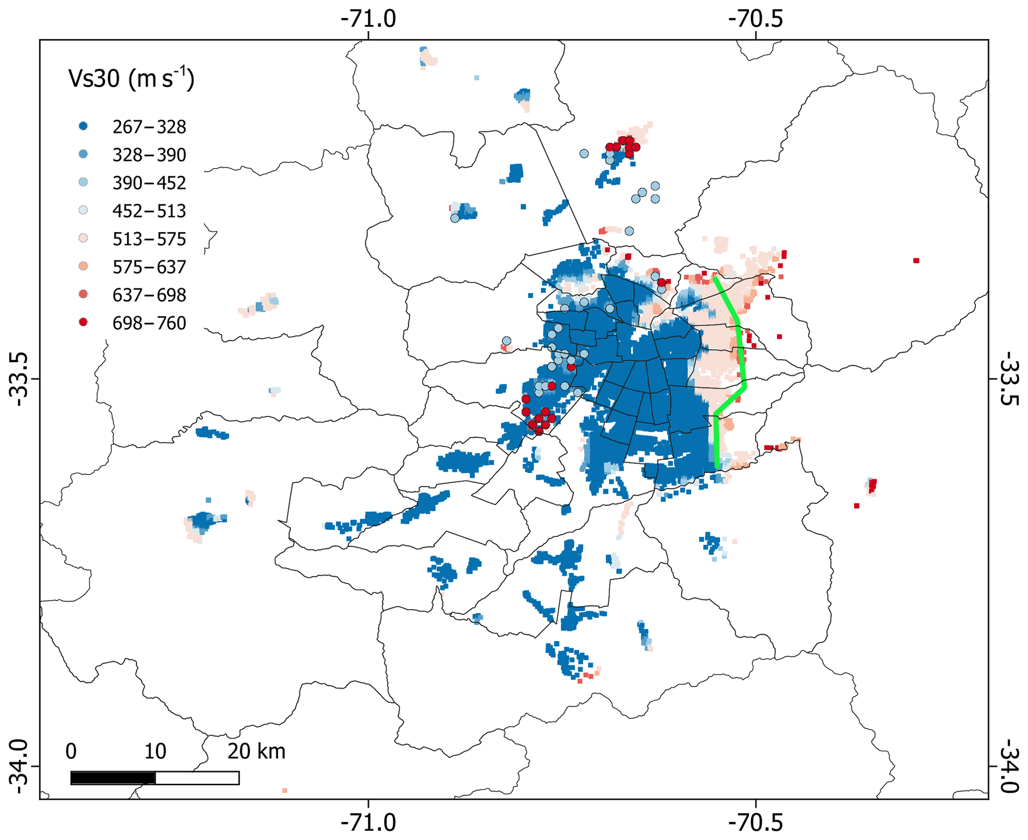
Figure 8A map of the Vs30: shear-wave velocity in the top 30 m of soil in metres per second at the exposure locations. The circled data are from microzonation studies (Leyton et al., 2011; Humire-Guarachi, 2013), and the remaining are estimates derived from the topographic slope (Allen and Wald, 2007). The green lines indicate the surface trace of the San Ramón Fault used in the seismic-risk-scenario calculations. Red colours indicate a relatively high Vs30 value and are generally in regions with exposed or shallow bedrock. Relatively slow Vs30 values are associated with sedimentary basins.
3.4 Building fragility and vulnerability models
The physical, or structural, vulnerability for a built system is defined as its susceptibility to losses when subjected to earthquake shaking. In our scenario calculations we use two main forms of vulnerability models: fragility functions, which are used to relate earthquake shaking to certain levels of physical damage to a building (e.g. extensive damage, collapse), and vulnerability functions (structural and occupants), which relate the earthquake shaking of a structure to the economic and human losses.
Villar-Vega et al. (2017) analytically derived fragility functions for the 57 building classes in the exposure dataset developed for the South America Risk Assessment (SARA) project (Yepes-Estrada et al., 2017). For our analysis we use the subset of these equations that represents the building exposure in the Santiago metropolitan region (Table 1 and Fig. S1). To derive the fragility functions, Villar-Vega et al. (2017) represented the structural capacity of each building class by a set of single-degree-of-freedom (SDOF) oscillators. Each oscillator was subjected to a suite of ground motion records representative of the South American tectonic environment and seismicity using GEM's Risk Modellers' Toolkit (Silva et al., 2015). From each analysis, the maximum spectral displacement of each SDOF oscillator was used to allocate it into a damage state (e.g. collapse). In this paper, we focus our scenario analysis on the spatial distribution of collapsed buildings, which comprises not only physically collapsed buildings but also partially collapsed structures (Villar-Vega et al., 2017).
The simplification of each building typology to a single-degree-of-freedom oscillator means that the calculated fragility functions only approximate the building response to ground shaking. Therefore these would not be sufficient to investigate building-by-building scale losses from earthquake shaking. However, we believe it is sufficient to explore aggregated district level losses. And so, while the scenario calculations are done on a 1 km×1 km gridded exposure model, the losses presented in the following sections aggregate these to the district level.
A vulnerability curve establishes the probability distribution of a loss ratio (e.g. fatalities / total number of occupants) given a shaking intensity measure level (Figs. 9 and S5). Vulnerability curves are generally empirically derived using loss data, usually collected through insurance claims or governmental reports. A database of fragility and vulnerability functions can be found in the OpenQuake platform (Yepes-Estrada et al., 2016; Martins and Silva, 2018). We used these vulnerability functions to directly model fatalities and repair costs, where the loss ratio for the former would be the ratio of fatalities to exposed population, and for the latter the ratio would be that of repair cost to cost of replacement for a given building typology.
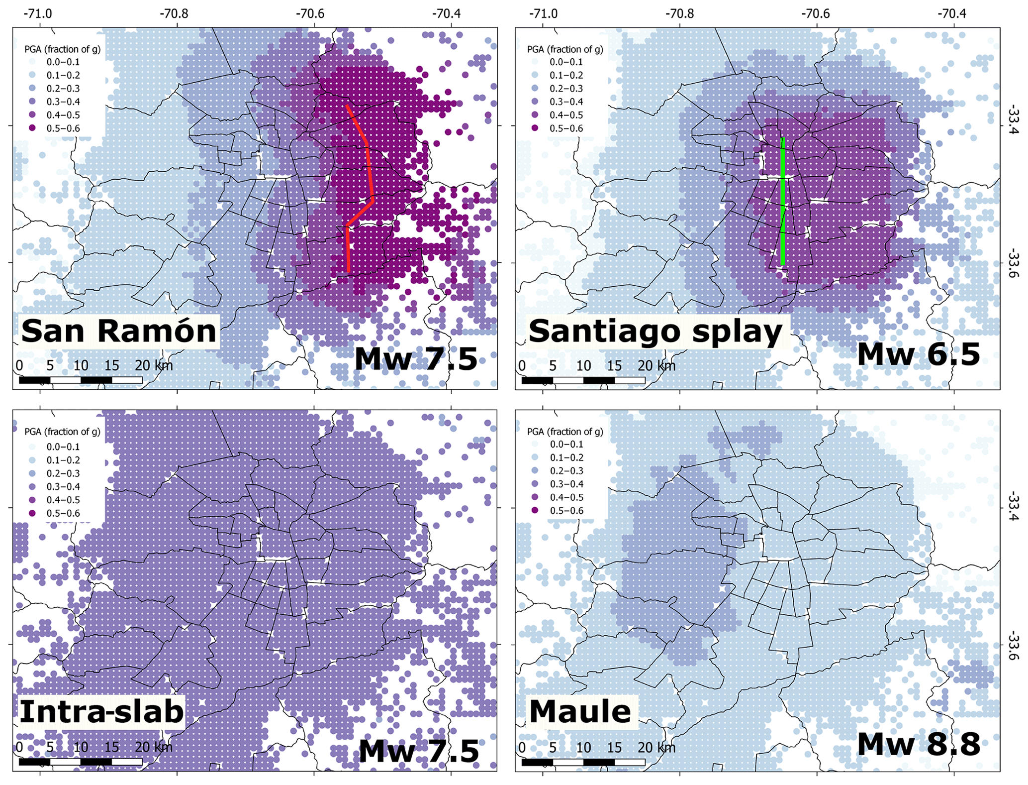
Figure 9The estimated median peak ground acceleration (PGA) as a fraction of gravity g for the largest earthquake scenario considered for each fault. For the San Ramón (red line) and Santiago splay fault (green line) cases, these estimates were obtained using the Akkar et al. (2014) ground motion prediction equation, while those for the intra-slab fault are estimates from the Abrahamson et al. (2016) equation. The USGS peak ground accelerations for the Mw 8.8 Maule earthquake are shown at the bottom. The ground motions for the full set of earthquake scenarios are given in Fig. S4.
3.5 Residential-building collapse and loss results
The median predicted ground motion for the larger earthquake scenario considered for each fault is given in Fig. 9. It shows the relatively simple ground motion patterns from the single rectangular Santiago splay fault and a more complex pattern from the San Ramón Fault. For the San Ramón case most of the high ground shaking is around the communes to the east of the city, while for the splay fault case there is a more even distribution of shaking across the central communes.
Our damage and loss results, averaged over the GMPEs used in each scenario calculation, reveal that the collapsed-building estimates for each scenario are distributed unevenly across the city (Fig. 10). Figure 11 shows a summary of the damage and loss results for all scenarios. It is clear that the damage and losses are greater for the larger-magnitude earthquake considered in each case as one would expect since larger earthquakes, at a given depth, produce higher-intensity ground shaking.
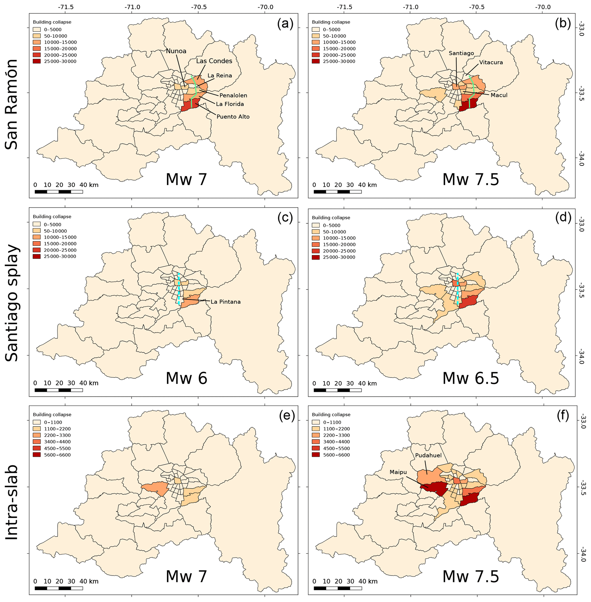
Figure 10The distribution of collapsed buildings for the earthquakes considered in each set of magnitude pair scenarios for the San Ramón Fault (green line; a–b), the Santiago splay fault (dashed cyan line; c–d), and a deep intra-slab fault (e–f). The collapse counts are the average for the GMPEs used in each calculation and include the total count of both complete and partial collapses. Note that the range of the colour scale changes between the upper four and lower two panels. The collapse fraction for each commune is given in the Supplement (Fig. S6). Names of all the communes are given in Fig. S1.
For the San Ramón scenarios the losses are mostly concentrated in the communes around the fault. Most collapsed buildings are located in Puente Alto (23 100–28 800; 16 %–20 %), La Florida (12 400–15 700; 15 %–19%), and Las Condes (10 500–12 800; 20 %–25 %), where the first numbers in the brackets are the building collapse counts for the two San Ramón Fault scenarios and the second two numbers the percentage of collapse of the total number of exposed buildings in the commune. We calculate fewer residential-building collapses in Peñalolén (5900–7400; 14 %–17 %) and La Reina (5000–6200; 18 %–23 %) despite these communes also being located on the fault. This discrepancy could be explained through a combination of greater exposed population – and thus more residential buildings (Fig. S6 shows the percentage of collapsed buildings) – and the level of poverty.
Puente Alto has the largest population of these communes (622 356) and also the greatest percentage living below the poverty line (Table 2). Puente Alto and La Florida also generally contain a greater proportion of masonry constructions (93 % and 86 % compared to 79 % and 71 % for Peñalolén and La Reina respectively), which perform poorly in the San Ramón earthquake scenarios. While Peñalolén has a low fraction of RC residential buildings (5 %), which generally perform well in our calculation, it is compensated by a large proportion of wooden structures (17 %), which perform the best when subject to seismic shaking.
Table 2Exposed populations and buildings for the 10 most affected communes in terms of average modelled building collapse across the six earthquake scenarios (full list in Supplement; Tables S2 and S3). The communes are ranked in order of average collapse count.
* defined as USD 400 monthly income (in 2015 US dollars) for a family of four (Ministerio de Desarrollo Social, 2016).
In general the greatest percentage of collapsed buildings (Fig. S6) occurs, as expected, in the communes directly on the fault, e.g. Vitacura (3000–3600; 21 %–25 %) and Las Condes (10 500–12 800; 20 %–25 %). However there are several communes with high collapse fractions that are not located on the fault, notably Ñuñoa (8400–10 600; 20 %–25 %) and Macul (4200–5300; 18 %–23 %). These both have a high fraction of unreinforced-masonry buildings, 27 % and 13 % respectively compared to an average of 9 % for the communes on the fault (Table 2). Unreinforced-masonry buildings are the most likely building class to collapse in all the scenarios considered in this study (Table 4).
In terms of anticipated fatalities for the larger San Ramón scenario (Fig. 12), the communes of Ñuñoa and Providencia (10 km west of the San Ramón fault trace) are modelled as experiencing the highest fatality rates of 4–5 per 1000 per 1000 people (Fig. S7). In terms of absolute numbers, the largest number of fatalities (Fig. 12) occurs in Ñuñoa and Las Condes (1120–1420 and 1080–1330 respectively). Overall the fatalities across the region are estimated in the range of 9700–12 700 (Fig. 11), resulting in a fatality rate of 0.15 %–0.19 % (Table S3). The residential losses in terms of replacement costs average USD 8–10 billion (5 %–7 % mean loss ratio). The greatest replacement costs are for Santiago (USD 1.3 billion), but they are also high (USD 0.5+ billion) for the communes of Puente Alto, Las Condes, and La Florida on top of the San Ramón Fault, as well as for Ñuñoa further west (Fig. S8).
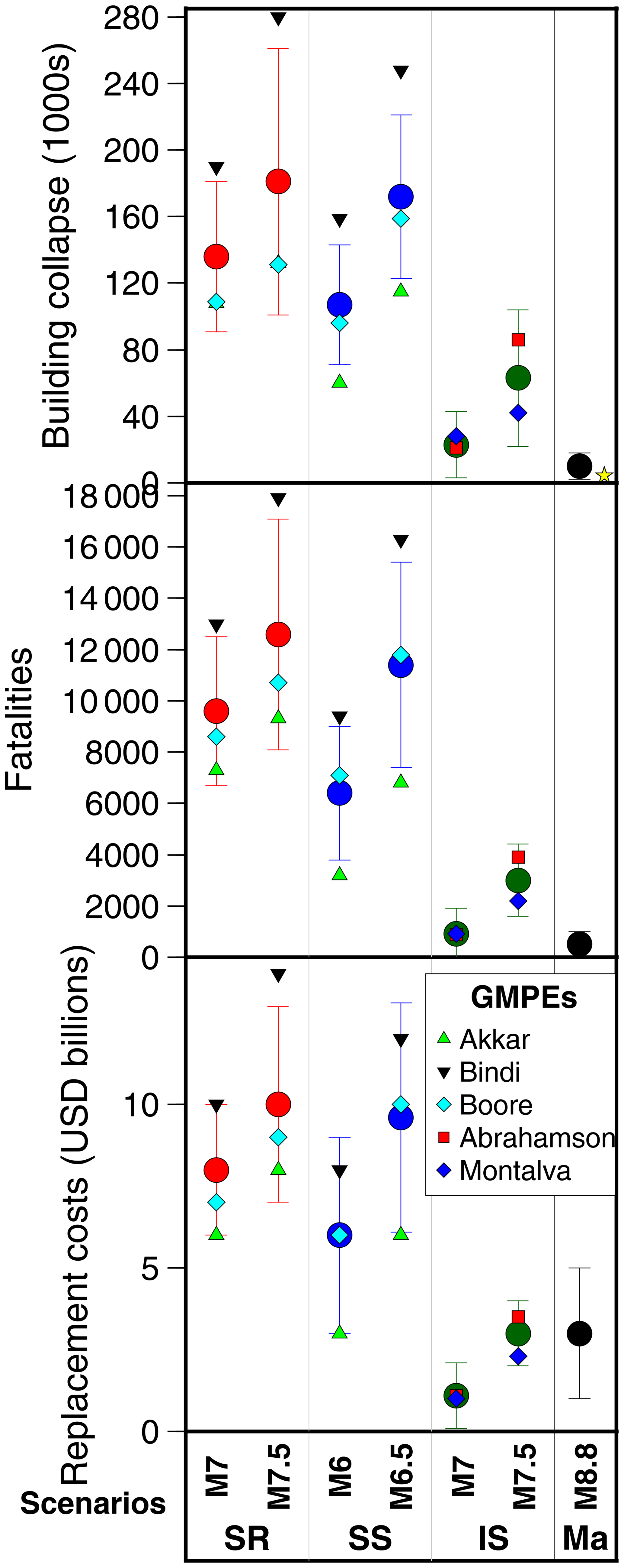
Figure 11A summary of the total number of building collapses and fatalities as well as the total replacement costs for each scenario calculation. The solid circles are the average across the GMPEs considered in each scenario, which are indicated by the smaller polygons. The spread in the estimates from the GMPEs indicates the epistemic uncertainty in our calculations. Error bars represent 1 standard deviation determined from the 1000 Monte Carlo simulations. The yellow star denotes the actual number of building collapses (4306) in Santiago in the 2010 Maule earthquake (Elnashai et al., 2010).
For the earthquake scenarios on a buried fault splay beneath the centre of the city, the distribution of collapsed residential buildings is similar to the San Ramón scenario with damage concentrated towards the eastern communes of the city on the hanging wall of the fault. Most collapses occur in Puente Alto (13 600–20 900; 9 %–15 %) and Santiago (10 000–15 400; 17 %–27 %). As in the case of the San Ramón Fault the high collapse count in Puente Alto probably reflects the large number of residential buildings in that commune. Of the communes directly next to the fault splay, Santiago has the largest number of residential buildings (57 341). However, the greatest impact in terms of collapse fraction is in the communes in the central districts near the fault, with the highest fraction of collapse occurring in Santiago (10 000–15 400; 17 %–27 %), Providencia (3400–5500; 15 %–25 %), Independencia (2500–3700; 16 %–24 %), and Ñuñoa (6600–10 300; 15 %–24 %). The estimated fatalities for the buried splay scenarios are similar to or slightly above those for the San Ramón cases despite being a magnitude lower in scale, in the range of 6500–11 500 (0.10 %–0.17 % loss ratio). The most affected communes are also similar, including Santiago, San Miguel, Providencia, and Ñuñoa, with fatality fractions of 4–5 per 1000 for the larger Mw 6.5 scenario (Fig. S7). The greatest number of fatalities for both magnitudes (Fig. 12) is also in Santiago and Ñuñoa (870–1600 and 710–1310 respectively; Table S3). The residential replacement costs are USD 6.1–9.6 billion (4 %–6 % loss ratio) for the two magnitude scenarios (Table S3). The greatest losses are in Santiago, Ñuñoa, and Puente Alto (Fig. S8).
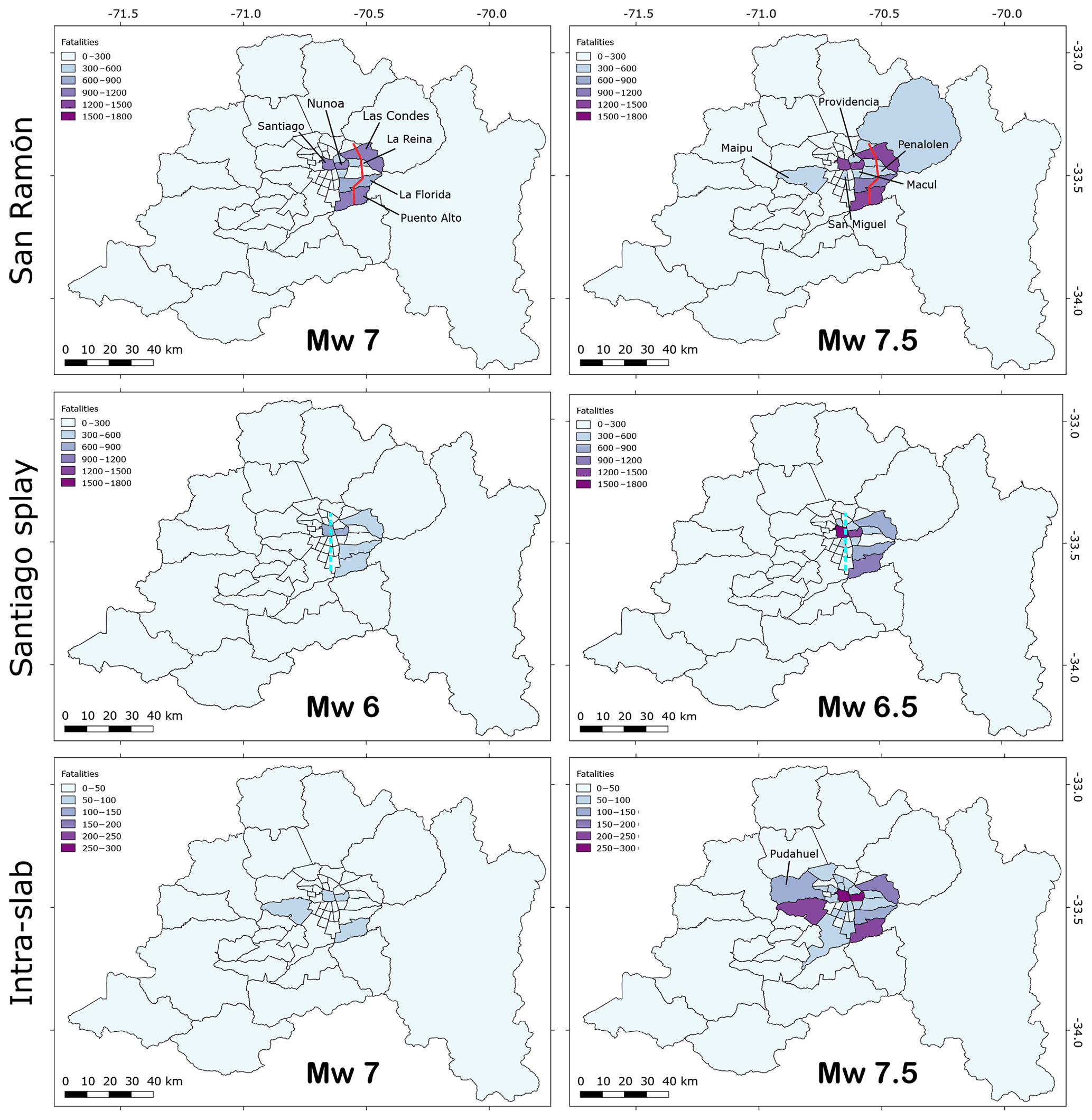
Figure 12The estimated fatalities in each commune for the earthquakes considered in each scenario for the San Ramón Fault (red line), the Santiago splay fault (dashed cyan line), and a deep intra-slab fault. Note that the range of the colour scale changes between the upper four and lower two panels.
The overall collapse count for the magnitude 7 deep intra-slab scenario is small, but the magnitude 7.5 scenario results in a substantial number of collapsed buildings (about 60 000), with most collapsed homes and fatalities (Fig. 12) generally located in the more populous communes. The extent of collapse across the city is more diffusive due to the buried nature of the intra-slab source, with building collapse up to 8% in the centre (Lo Espejo, San Joaquin, and Independencia). The estimated total number of fatalities (Fig. 11) for the larger event is 3180 (0.05 %), with the largest number of fatalities (200–300; Table S3) each in Santiago, Ñuñoa, Maipú, and Puente Alto (Fig. 12). The estimated replacement cost is USD 3 billion (2 % loss ratio), with the greatest costs distributed in the same commune as fatalities (Fig. S8).
Central government statistics estimate a total collapse count of 81 444 residential buildings throughout Chile in the 2010 Mw 8.8 earthquake, with the most damage occurring in the Maule, Biobío, O'Higgins, and Santiago metropolitan regions (Elnashai et al., 2010; de la Llera et al., 2017) and 4306 of these collapses occurring in the Santiago metropolitan region (yellow star in Fig. 11). While the collapse count is smaller than our modelled estimate of 9800±8000, it is within the error margin. The discrepancy could have arisen due to a slightly different exposure model. The actual exposure in 2010 would have been different than our exposure model estimates, which use data from 2014. Moreover, there is often ambiguity regarding the classification of actual structural collapse and damage beyond repair (and thus in need of demolition). See Villar-Vega et al. (2017) for a discussion on this topic.
While we estimate building collapse fractions up to 21 % (Providencia) for the Mw 7 San Ramón scenario, the average collapse ratio across all the communes is ∼8 %. This is larger than the 6.5 % estimated by Vaziri et al. (2012) for a magnitude 6.8 earthquake on the fault. However, their estimate of 14 000 fatalities is larger than the 9700 we estimate for a Mw 7 earthquake. This difference is most likely due to variations in the exposure model and calculation procedure (i.e. choice of ground motion models). But since Vaziri et al. (2012) used an industry exposure model we are not able to determine the exact cause behind the difference in our estimates.
In general, across all the scenarios considered in this study, the largest number of collapsed buildings occurs in the highly populous communes (which therefore have more buildings) close to the fault. However, the collapse and fatality fractions (the number of collapses or fatalities over the exposure; Figs. S6 and S7) reveal particularly vulnerable areas. Several communes experience relatively large damage and loss fractions, which is an indication of the vulnerability of the communities in these communes. Of particular importance are Ñuñoa, Providencia, and Santiago, which generally have high loss fractions with 3, 3, and 2 fatalities per 1000 people and damage fractions of 15 %, 15 %, and 15 % respectively, averaged over the six earthquake scenarios. In comparison the average loss fraction across all communes and all scenarios is 0.8 fatalities per 1000 people and 7 % building collapse. Therefore targeted measures to retrofit particularly vulnerable residential buildings (unreinforced masonry) could reduce the seismic risk faced by communities living in these communes.
We also used Risk Management Solutions' (RMS) commercial Chile Earthquake Model, developed in 2011, with the most recent industry exposure database (IED) to derive industry loss estimates for specific earthquake scenarios. The exposure model contains only non-residential-building information and does not include public infrastructure such as roads or bridges. The exposed values (or “total insured value”, TIV) in this dataset include commercial buildings, contents, and business interruption and are aggregated at the commune level.
Table 3Gross loss (GR) ratios for the Santiago non-residential exposure.
Table 3 and Fig. 13a give a summary of the average gross loss ratios (calculated loss over the total insured value) for the maximum-magnitude scenarios on the San Ramón and Santiago splay faults. The gross losses are the full replacement costs for the property after accounting for insurance penetration and after the application of deductibles, limits, and co-insurance. This is often referred to as the insured loss. It is worth noting that these losses are a subset of the full economic losses in an earthquake since the gross losses account for insurance penetration, which is always less than 100 %. The average insurance penetration (residential and non-residential) in the Santiago metropolitan region was 31.5 % in 2011. However, only an estimated 30 % of small commercial business owners had earthquake insurance, which rises to greater than 75 % for large commercial and industrial facilities (Muir-Wood, 2011).
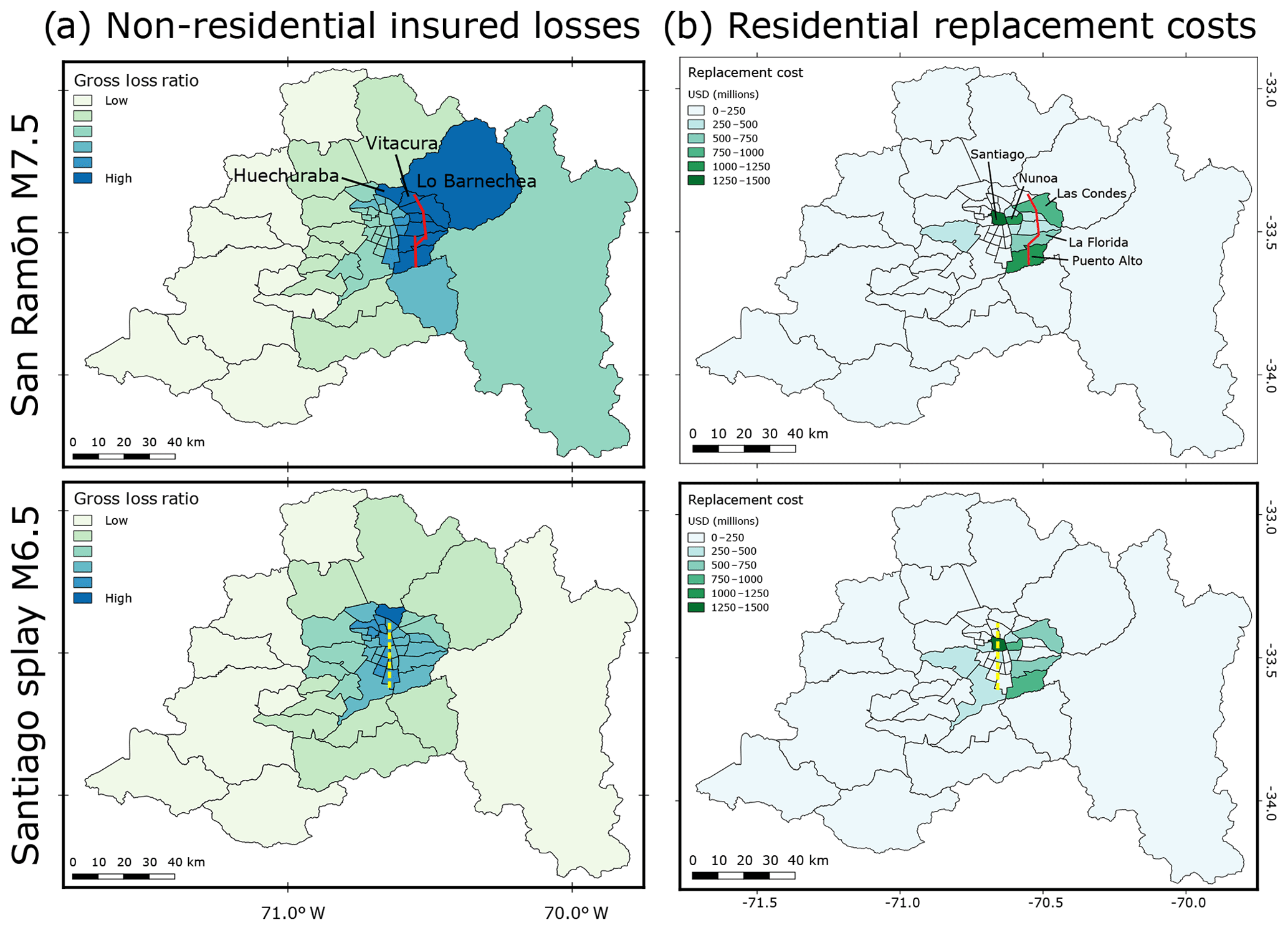
Figure 13The distribution of (a) non-residential and (b) residential replacement costs for maximum-magnitude scenarios considered for the San Ramón Fault and the Santiago splay fault (moment magnitude 7.5 and 6.5 respectively). The gross loss ratios represent the calculated losses in each scenario over the total insured value after the application of policy conditions and deductibles. The residential replacement costs are the costs to repair or replace buildings and their contents damaged in each scenario. The residential replacement cost maps for all scenarios are given in Fig. S8.
Whilst a detailed past record of earthquakes and variability of recurrence on the San Ramón Fault is not precisely known, the palaeo-seismic work of Vargas et al. (2014) tentatively points towards a recurrence interval of the order of ∼8 kyr; determined from records of two past earthquakes 17–19 and ∼8 kyr ago. Given that the last event was ∼8 kyr ago it is prudent to consider a San Ramón rupture scenario of Mw 7.5 as a real possibility to plan for. Vargas et al. (2018) find that present urbanisation of eastern Santiago reached 55 % of the San Ramón fault trace, evidencing that this active geological structure has not been considered in urban regulations developed for the metropolitan region.
5.1 Residential collapse by building class
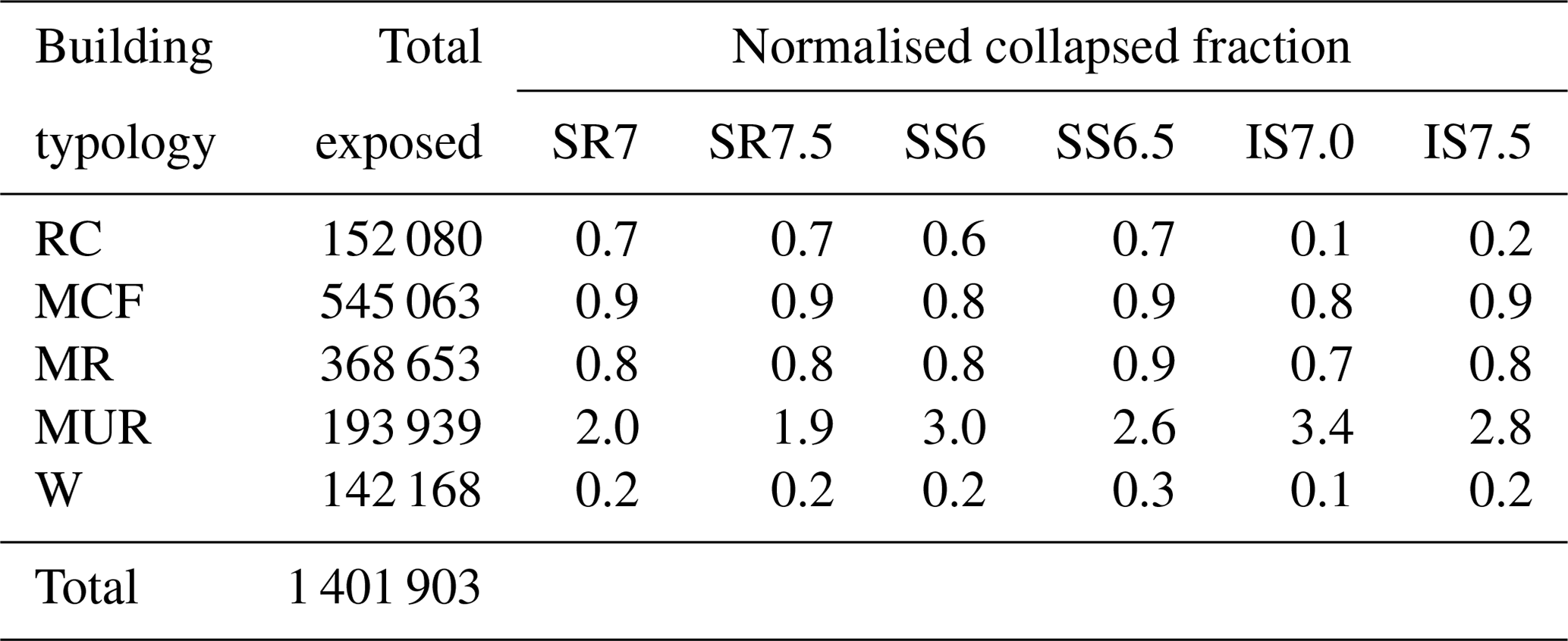
Buildings of differing construction material type are known to perform markedly differently under seismic shaking (Park and Hamza, 2016). We aim to identify the expected better- and less-well-performing building classes exposed in Santiago under our varying earthquake shaking scenarios. In order to compare the collapse ratios for the different building classes defined in Table 1 (RC, MCF, MR, MUR, and W), we calculate the normalised collapse fraction, NCF, for each building class according to
where et is the number of exposed residential buildings of building class t, and is the number of collapsed buildings of the same class in earthquake scenario s. Cs is the total number of collapsed buildings in scenario s, and E is the total number of exposed buildings in the city.
Therefore, if NCFt>1, then typology t is more likely to collapse than the average. The results of this normalisation are shown in Table 4. Across the six earthquake scenarios, we find that reinforced-concrete (RC) residential buildings perform best with a normalised collapse fraction NCFRC=0.5. It is also clear that unreinforced-masonry (MUR) structures collapse the most across all scenarios, with an average NCFMUR=2.6, implying that MUR structures are over 2.5 times more likely to collapse than the average. Typically, 3 %–13 % of buildings in the most affected communes (Table 2) are unreinforced-masonry constructions except for Santiago and Macul, where 27 % of the buildings are MUR. This is why we typically observe relatively large collapse fractions in Santiago (1700–15 400; 3 %–27 %) and to a lesser extent Macul (600–5300; 3 %–23 %) over the six earthquake scenarios considered in this study. Wooden residential homes (W) perform very well with an average NCFW=0.2. Confined-masonry (NCFMCF=0.9) and reinforced-masonry (NCFMR=0.8) perform better than unreinforced-masonry buildings and slightly better than the average. It is clear that masonry construction in general performs worse during earthquakes.
Table 4The fraction of collapsed residential buildings by building class (Table 1) normalised to the total collapse fraction in each earthquake scenario. SR: San Ramón; SS: Santiago splay; IS: intra-slab. The number indicates the moment magnitude of the earthquake source. Values greater than 1 indicate that the building typology is more likely to collapse than the average.
5.2 Magnitude–distance trade-off
The calculated collapses and losses for each of the scenarios using the residential-building exposure show the expected pattern of greater losses for a larger earthquake on a given fault (Fig. 11 and Table 5). Our calculations show that the San Ramón earthquake scenarios are the most damaging to the city, with 136 400 residential-building collapses from a magnitude 7 and 181 300 collapses from a magnitude 7.5 earthquake on the fault, a difference of 25 %. The estimated damage from the buried Santiago splay fault comprises 107 300 collapses for a magnitude 6 and 172 200 collapses for a magnitude 6.5 earthquake, a difference of 38 %. We note a similar pattern in the losses, with an increase of 24 % and 20 % in fatalities and replacement cost respectively between a magnitude 7 and 7.5 earthquake on the San Ramón Fault and an increase of 38 % and 43 % on the splay fault earthquakes. It is clear from our calculations that a half magnitude increase in earthquake size results in more damages and losses from the Santiago splay fault than the San Ramón Fault. This is probably because shaking from the splay fault exposes more of the densely populated communes in the centre of the city, where a small increase in shaking can have more impact.
Table 5Summary of losses from each fault and earthquake scenario.
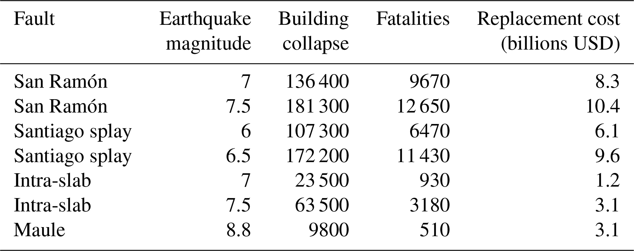
In all cases, the magnitude 8.8 Maule earthquake produces fewer losses to the city than the smaller local earthquakes despite having 100–10 000 times the moment release of the other scenarios considered here. According to our models, it is clear that there is a trade-off between earthquake magnitude and distance in terms of residential-building collapses and fatalities. Chatelain et al. (1999) also found a similar trade-off in their earthquake risk assessment for Quito, Ecuador. Therefore, simply focussing on large offshore megathrust earthquakes would mask the significant risks posed from moderate-size earthquakes on smaller but more local active faults.
5.3 Residential and non-residential insured losses
Figure 13b shows the loss distribution of the residential-building replacement costs due to a magnitude 7.5 earthquake on the San Ramón Fault and a magnitude 6.5 earthquake on a buried splay fault beneath the centre of the city. While these are not directly comparable with the non-residential insured losses (Fig. 13a), partly due to the fact that the insured losses are impacted by insurance penetration and also include business interruption and policy conditions, there are some clear differences between the two that are worth noting.
For the San Ramón scenario the highest residential-building replacement costs are generally concentrated in the communes with large populations (hence more residential buildings) close to the fault and those with a large fraction of reinforced-concrete buildings, which are more expensive than masonry structures. The greatest losses occur in Puente Alto, La Florida, Las Condes, and Santiago, while the insured losses were equally high in all communes along the fault, including high loss ratios in Lo Barnechea and Huechuraba, two communes not directly above the fault.
This difference reflects the concentration of high-value commercial properties in the more affluent eastern communes, where businesses are more likely to be insured (Muir-Wood, 2011), particularly in Las Condes and La Reina. The residential losses reflect the damages in highly populous communes, as evidenced by the losses in Santiago, Ñuñoa, and La Florida.
Similarly the losses in residential buildings for a magnitude 6.5 earthquake on the Santiago splay are concentrated in the eastern communes on the hanging wall of the fault (Santiago, Ñuñoa, and Puente Alto), while the insured losses concentrate around the central business districts of Santiago and Huechuraba.
5.4 Caveats and limitations
There are a number of caveats and sources of uncertainty in estimating damage and losses from past and hypothetical earthquake scenarios using the method described in this paper. One of the main sources of uncertainty is the exposure model, which does not exactly correspond to the exposed population and building portfolio that were affected by a past earthquake. For this study the exposure model was developed by Santa-María et al. (2017) using information from census surveys and housing information from 2014. Therefore, it is important to note that the exposure model used in investigating the damage and losses for the hypothetical earthquake scenarios on the San Ramón Fault, Santiago splay, and deep intra-slab faults does not represent the exact current exposure of the Santiago metropolitan region. This is particularly important for Santiago, where rapid eastward expansion of the city into the foothills of the San Ramón mountains puts an increasingly greater population closer to the San Ramón Fault (Fig. 1) and onto its hanging wall, where ground accelerations are typically higher. Therefore, methods that allow for a near-continuous update of building inventories and locations are needed to maintain the veracity of exposure.
One of the largest sources of uncertainty in the calculations is in the GMPEs. In order to capture the epistemic uncertainty in both median ground motion predictions and their associated aleatory variability, we used several equally weighted GMPEs (e.g. Bommer et al., 2005, 2010). The differences in the datasets used to derive each GMPE and the way each GMPE calculates the ground motions are partly why the uncertainty range in our estimates of the number of collapsed buildings is large (Fig. 11).
The development of fragility models also involves large uncertainties. The fragility functions used in this study were developed using a probabilistic approach where a set of structures are tested against a suite of ground motion records (Villar-Vega et al., 2017). Since it is time- and cost-prohibitive to develop a fragility function for every building in the city, each of the buildings is allocated to a building typology within a general building class in the exposure model. Each typology is then represented by a single-degree-of-freedom block to calculate its response to the ground motion records. It is important to note that this level of simplification adds uncertainty in the final response of any particular typology in the event of an earthquake (see Villar-Vega and Silva, 2017, for a discussion). Also, it is not possible to say how any individual building will respond to an earthquake using this approach as the fragility functions do not include the unique complexities in the design and construction of every building.
The results shown in this paper are from scenario-based calculations on predetermined faults, and thus we cannot provide the relative likelihood of a shaking event as in a probabilistic seismic-hazard analysis (PSHA) framework. However, this is an important start to motivate continued work on the recurrence interval of faults in the region, begun by Armijo et al. (2010) and Vargas et al. (2014) on the San Ramón Fault. The SPOT DEM is not good enough to conclusively identify the presence of any geomorphic marker that may result from a splay fault within the city. Its very existence, let alone relative level of activity, remains an open question. Higher-resolution DEMs or detailed field surveys might be able to resolve this issue.
It is important to note that although the focus of this paper has been to explore the direct damage and losses due to earthquakes, in the case of an actual event there are often cascading hazards in the form of liquefaction, tsunamis, landslides, and blocked waterways leading to floods, fires, etc. that can lead to loss of lives and livelihoods (Gill and Malamud, 2014). Nevertheless, historically most fatalities in earthquakes were due to direct building collapse apart from the large tsunami death tolls from a few 21st-century megathrust earthquakes (Ambraseys and Bilham, 2011).
In this study we use high-resolution DEMs of the metropolitan area of Santiago city and the foothills of the San Ramón mountains created using SPOT and Pléiades satellite imagery to accurately map the surface expression and segmentation of the San Ramón Fault. We recognise that estimates of the impact from specific earthquakes (historical or hypothetical) can support decision makers in the development of risk reduction strategies. We therefore use the OpenQuake Engine to calculate damage and losses for realistic earthquake scenarios on the mapped San Ramón Fault as well as a potential unknown fault, buried directly beneath the centre of the city, and a deep intra-slab fault. We compare these losses with those for the 2010 magnitude 8.8 offshore Maule earthquake as a reference level of a recent event. Our calculations show that there is a strong magnitude–distance trade-off in terms of direct damage to the exposed building portfolio and fatalities, with smaller, more local shallow earthquakes causing greater losses to the city than a larger offshore megathrust earthquake. It is clear that the eastward expansion of the city into the foothills of the San Ramón mountains has exposed a large number of (predominantly affluent) people to a future earthquake on the San Ramón Fault. While the recurrence interval of large earthquakes on the fault are long (∼8 kyr) and only very loosely constrained, the last Mw 7.5 event was ∼8 kyr ago (Vargas et al., 2014). So it is prudent to consider the potential impacts of a San Ramón rupture scenario of similar magnitude. We calculate losses using scenario-based models of San Ramón earthquake ruptures in the magnitude range of 7–7.5 under the current residential exposure. Our models estimate 181 000±80 000 partial to total building collapses, 12 700±4500 fatalities, and replacement costs of USD 10±3 billion for the larger-magnitude earthquakes the San Ramón Fault can accommodate, assuming all fault segments fail at once. While these numbers are subject to considerable uncertainty arising from a changing exposure as well as from uncertain ground motion prediction equations and fragility functions, they provide an informative guide to the potential scale of losses from a large earthquake on the San Ramón Fault. For all modelled scenarios, the most vulnerable building class is unreinforced masonry, while wooden structures and reinforced concrete are the most resilient to earthquake shaking. Therefore, effective near-term risk reduction measures could target unreinforced-masonry homes for retrofitting campaigns, particularly in Ñuñoa, Providencia, and Santiago, while in the mid to long term a drive towards reinforced-concrete homes would significantly reduce the risks to future earthquakes from both near- and far-field sources. This work also reinforces the need to identify active faults adjacent to or beneath cities in actively deforming zones and the need to update the exposure models as such cities encroach onto these faults. We have highlighted that local crustal earthquakes in the magnitude range of 6–7.5 can have a much greater impact than larger distant earthquakes. Therefore the frequency of major distal earthquakes has to be balanced by the potential for infrequent but much more potent, smaller local earthquakes on less active faults.
The latest version of the OpenQuake Engine can be downloaded from the Global Earthquake Model GitHub repository: https://github.com/gem/oq-engine (GEM, 2019). The point clouds created from both the SPOT and Pléiades stereo satellite imagery have been uploaded to the OpenTopography platform (http://opentopography.org, last access: May 2020) and are available to download for free.
The supplement related to this article is available online at: https://doi.org/10.5194/nhess-20-1533-2020-supplement.
EH conducted the research and wrote the manuscript. JRE devised and led the project and assisted with the satellite data acquisition, analysis, and manuscript writing. VS and MVV assisted with the residential seismic risk calculations. DK provided the non-residential risk calculation results. All authors contributed to discussions and manuscript preparation.
Any opinions, findings, conclusions, or recommendations expressed in this paper are those of the authors and do not necessarily reflect those of Risk Management Solutions, Inc.
This work has been supported by the NERC/AHRC/ESRC Global Challenges Research Fund (GCRF) awarded to the Seismic Cities project (grant number NE/P015964/1), by the Royal Society GCRF Challenge grant (CHG\R1\170038), and in part by the British Geological Survey (BGS) Overseas Development Assistance programme (NEE6214NOD). This paper is published with the approval of the BGS Executive Director. We would like to thank the Seismic Cities team for helpful discussions, especially Paula Repetto for help in accessing the Chilean datasets. The lead author would like to thank Catalina Yepes-Estrada, Anirudh Rao, and Marco Pagani, as well as all other members of the GEM Hazard and Risk team for their patience in explaining the details and methodologies of the OpenQuake Engine. The lead author would also like to thank the Research Center for Integrated Disaster Risk Management (CIGIDEN) in Chile for hosting the January 2017 OpenQuake Engine training workshop. We also thank Tim Craig for suggesting the need to also consider intra-slab earthquakes as potential major shaking sources and Laura Gregory for help with interpreting fault profiles. We thank colleagues at RMS, including Justin Moresco, Chesley Williams, and Robert Muir-Wood. We gratefully acknowledge the CEOS Seismic Pilot for providing the Pléiades stereo imagery over the San Ramón Fault (© CNES, 2016; distribution Airbus DS/Spot Image). Pléiades images made available by CNES in the framework of the CEOS WG Disasters. JRE is supported by a Royal Society University Research fellowship (UF150282).
This work has been supported by the NERC/AHRC/ESRC Global Challenges Research Fund (GCRF) awarded to the Seismic Cities project (grant no. NE/P015964/1), by the Royal Society GCRF Challenge (grant no. CHG\R1\170038), and in part by the British Geological Survey (BGS) Official Development Assistance programme (grant no. NEE6214NOD).
This paper was edited by Uwe Ulbrich and reviewed by Robin Lacassin and one anonymous referee.
Abrahamson, N., Gregor, N., and Addo, K.: BC Hydro ground motion prediction equations for subduction earthquakes, Earthq. Spectra, 32, 23–44, 2016. a, b
Akkar, S., Sandıkkaya, M., and Bommer, J.: Empirical ground-motion models for point-and extended-source crustal earthquake scenarios in Europe and the Middle East, B. Earthq. Eng., 12, 359–387, 2014. a, b
Allen, T. I. and Wald, D. J.: Topographic slope as a proxy for seismic site-conditions (Vs30) and amplification around the globe, Tech. rep., United States Geological Survey (USGS), available at: https://pubs.usgs.gov/of/2007/1357/pdf/OF07-1357_508.pdf (last access: 1 March 2018), 2007. a, b
Ambraseys, N. and Bilham, R.: Corruption kills, Nature, 469, 153–155, , 2011. a
Armijo, R., Rauld, R., Thiele, R., Vargas, G., Campos, J., Lacassin, R., and Kausel, E.: The West Andean thrust, the San Ramon fault, and the seismic hazard for Santiago, Chile, Tectonics, 29, TC2007, https://doi.org/10.1029/2008TC002427, 2010. a, b, c, d, e, f, g, h, i, j, k
Armijo, R., Lacassin, R., Coudurier-Curveur, A., and Carrizo, D.: Coupled tectonic evolution of Andean orogeny and global climate, Earth-Sci. Rev., 143, 1–35, 2015. a, b
Barka, A., Akyuz, H. S., Altunel, E., Sunal, G., Cakir, Z., Dikbas, A., Yerli, B., Armijo, R., Meyer, B., de Chabalier, J. B., Rockwell, T., Dolan, J. R., Hartleb, R., Dawson, T., Christofferson, S., Tucker, A., Fumal, T., Langridge, R., Stenner, H., Lettis, W., Bachhuber, J., and Page, W.: The surface rupture and slip distribution of the 17 August 1999 Izmit earthquake (M 7.4), North Anatolian fault, B. Seismol. Soc. Am., 92, 43–60, 2002. a
Beck, S., Barrientos, S., Kausel, E., and Reyes, M.: Source characteristics of historic earthquakes along the central Chile subduction Askew et Alzone, J. S. Am. Earth Sci., 11, 115–129, 1998. a, b
Bilham, R.: Lessons from the Haiti earthquake, Nature, 463, 878–879, https://doi.org/10.1038/463878a, 2010. a
Bindi, D., Massa, M., Luzi, L., Ameri, G., Pacor, F., Puglia, R., and Augliera, P.: Pan-European ground-motion prediction equations for the average horizontal component of PGA, PGV, and 5 %-damped PSA at spectral periods up to 3.0 s using the RESORCE dataset, B. Earthq. Eng., 12, 391–430, 2014. a
Bommer, J. J., Scherbaum, F., Bungum, H., Cotton, F., Sabetta, F., and Abrahamson, N. A.: On the use of logic trees for ground-motion prediction equations in seismic-hazard analysis, B. Seismol. Soc. Am., 95, 377–389, 2005. a
Bommer, J. J., Douglas, J., Scherbaum, F., Cotton, F., Bungum, H., and Fäh, D.: On the selection of ground-motion prediction equations for seismic hazard analysis, Seismol. Res. Lett., 81, 783–793, 2010. a
Boore, D. M., Stewart, J. P., Seyhan, E., and Atkinson, G. M.: NGA-West2 equations for predicting PGA, PGV, and 5 % damped PSA for shallow crustal earthquakes, Earthq. Spectra, 30, 1057–1085, 2014. a
Chatelain, J.-L., Tucker, B., Guillier, B., Kaneko, F., Yepes, H., Fernandez, J., Valverde, J., Hoefer, G., Souris, M., Dupérier, E., Yamada, T., Bustamante, G., and Villacis, C: Earthquake risk management pilot project in Quito, Ecuador, GeoJournal, 49, 185–196, 1999. a
Chaulagain, H., Rodrigues, H., Silva, V., Spacone, E., and Varum, H.: Earthquake loss estimation for the Kathmandu Valley, B. Earthq. Eng., 14, 59–88, 2016. a, b
Civico, R., Pucci, S., Villani, F., Pizzimenti, L., De Martini, P. M., Nappi, R., and Group, O. E. W.: Surface ruptures following the 30 October 2016 Mw 6.5 Norcia earthquake, central Italy, J. Maps, 14, 151–160, 2018. a
Comte, D., Eisenberg, A., Lorca, E., Pardo, M., Ponce, L., Saragoni, R., Singh, S., and Suárez, G.: The 1985 central Chile earthquake: A repeat of previous great earthquakes in the region?, Science, 233, 449–453, 1986. a
Dahlen, F.: Critical taper model of fold-and-thrust belts and accretionary wedges, Annu. Rev. Earth Pl. Sc., 18, 55–99, 1990. a, b
Davis, D., Suppe, J., and Dahlen, F.: Mechanics of fold-and-thrust belts and accretionary wedges, J. Geophys. Res.-Sol. Ea., 88, 1153–1172, 1983. a
de Ballore, F. D. M.: Historia sísmica de los Andes Meridionales al sur del paralelo XVI, Anales de la Universidad de Chile, 9–63, 1913 (in Spanish). a
de la Llera, J. C., Rivera, F., Mitrani-Reiser, J., Jünemann, R., Fortuño, C., Ríos, M., Hube, M., Santa María, H., and Cienfuegos, R.: Data collection after the 2010 Maule earthquake in Chile, B. Earthq. Eng., 15, 555–588, 2017. a
DeMets, C., Gordon, R. G., and Argus, D. F.: Geologically current plate motions, Geophys. J. Int., 181, 1–80, 2010. a
Douglas, J. and Edwards, B.: Recent and future developments in earthquake ground motion estimation, Earth-Sci. Rev., 160, 203–219, 2016. a
Elliott, J., Nissen, E., England, P., Jackson, J. A., Lamb, S., Li, Z., Oehlers, M., and Parsons, B.: Slip in the 2010–2011 Canterbury earthquakes, New Zealand, J. Geophys. Res..-Sol. Ea., 117, B03401, https://doi.org/10.1029/2011JB008868, 2012. a
Elliott, J., Walters, R., and Wright, T.: The role of space-based observation in understanding and responding to active tectonics and earthquakes, Nat. Commun., 7, 13844, https://doi.org/10.1038/ncomms13844, 2016. a
Elnashai, A. S., Gencturk, B., Kwon, O.-S., Al-Qadi, I. L., Hashash, Y., Roesler, J. R., Kim, S. J., Jeong, S.-H., Dukes, J., and Valdivia, A.: The Maule (Chile) earthquake of February 27, 2010: Consequence assessment and case studies, Tech. rep., Mid-American Earthquake Center, Department of Civil and Environmental Engineering, University of Illinois at Urbana-Champaign, available at: http://hdl.handle.net/2142/18212 (last access, 1 June 2018), 2010. a, b
England, P. and Jackson, J.: Uncharted seismic risk, Nat. Geosci., 4, 348–349, https://doi.org/10.1038/ngeo1168, 2011. a
Estay, N. P., Yáñez, G., Carretier, S., Lira, E., and Maringue, J.: Seismic hazard in low slip rate crustal faults, estimating the characteristic event and the most hazardous zone: study case San Ramón Fault, in southern Andes, Nat. Hazards Earth Syst. Sci., 16, 2511–2528, https://doi.org/10.5194/nhess-16-2511-2016, 2016. a, b
Farías, M., Comte, D., Charrier, R., Martinod, J., David, C., Tassara, A., Tapia, F., and Fock, A.: Crustal-scale structural architecture in central Chile based on seismicity and surface geology: Implications for Andean mountain building, Tectonics, 29, TC3006, https://doi.org/10.1029/2009TC002480, 2010. a
Farr, T. G., Rosen, P. A., Caro, E., Crippen, R., Duren, R., Hensley, S., Kobrick, M., Paller, M., Rodriguez, E., Roth, L., Seal, D., Shaffer, S., Shimada, J., Umland, J., Werner, M., Oskin, M., Burbank, D., and Alsdorf, D.: The Shuttle Radar Topography Mission, Rev. Geophys., 45, RG2004, https://doi.org/10.1029/2005RG000183, 2007. a
Fischer, T., Alvarez, M., De la Llera, J., and Riddell, R.: An integrated model for earthquake risk assessment of buildings, Eng. Struct., 24, 979–998, 2002. a
Frohlich, C.: Deep earthquakes, Cambridge University Press, Cambridge, UK, 2006. a
Galetzka, J., Melgar, D., Genrich, J. F., Geng, J., Owen, S., Lindsey, E. O., Xu, X., Bock, Y., Avouac, J.-P., Adhikari, L. B., Upreti, B. N., Pratt-Sitaula, B., Bhattarai, T. N., Sitaula, B. P., Moore, A., Hudnut, K. W., Szeliga, W., Normandeau, J., Fend, M., Flouzat, M., Bollinger, L., Shrestha, P., Koirala, B., Gautam, U., Bhatterai, M., Gupta, R., Kandel, T., Timsina, C., Sapkota, S. N., Rajaure, S., and Maharjan, N.: Slip pulse and resonance of the Kathmandu basin during the 2015 Gorkha earthquake, Nepal, Science, 349, 1091–1095, 2015. a
GEM: The OpenQuake-engine User Manual, Global Earthquake Model (GEM) OpenQuake Manual for Engine version 3.3.2, Tech. rep., Global Earthquake Model (GEM), Pavia, Italy, GitHub, available at: https://github.com/gem/oq-engine, last access: 1 August 2019. a, b
Gill, J. C. and Malamud, B. D.: Reviewing and visualizing the interactions of natural hazards, Rev. Geophys., 52, 680–722, 2014. a
Grossi, P. and Kunreuther, H.: Catastrophe modeling: A new approach to managing risk, vol. 25, Springer Science & Business Media, 2005. a
Hayes, G. P., Wald, D. J., and Johnson, R. L.: Slab1.0: A three-dimensional model of global subduction zone geometries, J. Geophys. Res.-Sol. Ea., 117, B01302, https://doi.org/10.1029/2011JB008524, 2012. a, b
Humire-Guarachi, F. A. H.: Aplicación de métodos geofísicos basados en ondas superficiales para la caracterización sísmicade suelos. Aplicación a la microzonificación sísmica del norte y poniente de Santiago, Tech. rep., Pontifica Universidad Catolica de Chile, available at: https://tinyurl.com/vqfkauq (last access: 1 January 2019), 2013. a, b
Jayaram, N. and Baker, J. W.: Correlation model for spatially distributed ground-motion intensities, Earthquake Engineering & Structural Dynamics, 38, 1687–1708, 2009. a
Joyner, W. B.: Strong motion from surface waves in deep sedimentary basins, B. Seismol. Soc. Am., 90, S95–S112, 2000. a
Leyton, F., Sepúlveda, S. A., Astroza, M., Rebolledo, S., Acevedo, P., Ruiz, S., Gonzalez, L., and Foncea, C.: Seismic zonation of the Santiago basin, Chile, in: 5th International Conference on Earthquake Geotechnical Engineering, 2011. a, b
Lomnitz, C.: Major earthquakes and tsunamis in Chile during the period 1535 to 1955, Geol. Rundsch., 59, 938–960, 1970. a
Lomnitz, C.: On the epicenter of the great Santiago earthquake of 1647, B. Seismol. Soc. Am., 73, 885–886, 1983. a
Lomnitz, C.: Major earthquakes of Chile: A historical survey, 1535–1960, Seismol. Res. Lett., 75, 368–378, 2004. a
Martins, L. and Silva, V.: A Global Database of Vulnerability Models for Seismic Risk Assessment, in: Proceeding of the 16th European Conference on Earthquake Engineering, 2018. a
Ministerio de Desarrollo Social: Estimaciones de la pobreza por ingresos y multidimensional en comunas con representatividad, Tech. rep., Gobierno de Chile, available at: http://observatorio.ministeriodesarrollosocial.gob.cl/casen-multidimensional/casen/docs/estimacion_pobreza_ingreso_multidimensional_comunal.pdf (last access: 1 November 2018), 2016 (in Spanish). a, b, c
Montalva, G. A., Bastías, N., and Rodriguez-Marek, A.: Ground-Motion Prediction Equation for the Chilean Subduction Zone, B. Seismol. Soc. Am., 107, 901–911, https://doi.org/10.1785/0120160221, 2017. a
Muir-Wood, R.: Designing optimal risk mitigation and risk transfer mechanisms to improve the management of earthquake risk in Chile, OECD Working Papers on Finance, Insurance and Private Pensions, p. 1, 2011. a, b
Oncken, O., Hindle, D., Kley, J., Elger, K., Victor, P., and Schemmann, K.: Deformation of the central Andean upper plate system: Facts, fiction, and constraints for plateau models, in: The Andes, 3–27, Springer, https://doi.org/10.1007/978-3-540-48684-8_1, 2006. a
Park, R. and Hamza, M.: Earthquake Resistant Structures, in: Reference Module in Materials Science and Materials Engineering, Elsevier, https://doi.org/10.1016/B978-0-12-803581-8.00856-0, 2016. a
Pasten, C.: Respuesta sísmica de la cuenca de Santiago, Tech. rep., Facultad de Ciencias Físicas y Matemáticas. Santiago, Chile, available at: http://repositorio.uchile.cl/handle/2250/102937 (last access: 1 April 2020), 2007. a
Pérez, A., Ruiz, J., Vargas, G., Rauld, R., Rebolledo, S., and Campos, J.: Improving seismotectonics and seismic hazard assessment along the San Ramon Fault at the eastern border of Santiago city, Chile, Nat. Hazards, 71, 243–274, 2014. a, b, c
Pilz, M., Parolai, S., Stupazzini, M., Paolucci, R., and Zschau, J.: Modelling basin effects on earthquake ground motion in the Santiago de Chile basin by a spectral element code, Geophys. J. Int., 187, 929–945, 2011. a
Pina, F., Ventura, C., and Nunez, T.: Seismic Risk Assessment in Northern Chile – Lessons from a reconnaissance visit before the next mega-earthquake in Peru-Chile, in: Proceedings of the 15th World Conference on Earthquake Engineering, Lisbon, Portugal, 2012. a
Poirier, J.-P.: The 1755 Lisbon disaster, the earthquake that shook Europe, Eur. Rev., 14, 169–180, 2006. a
Ramón, A. d.: Santiago de Chile [1541–1991]: Historia de una sociedad urbana, MAPFRE, 1992 (in Spanish). a
Rauld, R.: Análisis morfoestructural del frente cordillerano de Santiago oriente, entre el Río Mapocho y la Quebrada de Macul (in Spanish), PhD thesis, Memoria de Título (Inédito), Universidad de Chile, Departamento de Geología, 2002. a
Reynolds, K., Copley, A., and Hussain, E.: Evolution and dynamics of a fold-thrust belt: The Sulaiman Range of Pakistan, Geophys. J. Int., 201, 683–710, 2015. a, b
Riesner, M., Lacassin, R., Simoes, M., Armijo, R., Rauld, R., and Vargas, G.: Kinematics of the active West Andean fold-and-thrust belt (central Chile): Structure and long-term shortening rate, Tectonics, 36, 287–303, 2017. a, b
Riley, S. J., DeGlioria, S. D., and Elliot, R.: Index that quantifies topographic heterogeneity, Intermountain Journal of Sciences, 5, 23–27, 1999. a
Saita, T.: The great Chilean earthquake of January 24, 1939, B. Earthq. Res. I. Tokyo, 18, 446–459, 1940. a
Santa-María, H., Hube, M. A., Rivera, F., Yepes-Estrada, C., and Valcárcel, J. A.: Development of national and local exposure models of residential structures in Chile, Nat. Hazards, 86, 55–79, 2017. a, b, c
Santos, S., Lima, S., and Arai, A.: Comparative study of codes for the seismic design of structures, Revista IBRACON de Estruturas e Materiais, 5, 812–819, 2012. a
Silva, V., Crowley, H., Pagani, M., Monelli, D., and Pinho, R.: Development of the OpenQuake engine, the Global Earthquake Model’s open-source software for seismic risk assessment, Nat. Hazards, 72, 1409–1427, 2014. a, b, c, d
Silva, V., Casotto, C., Rao, A., Villar, M., Crowley, H., and Vamvatsikos, D.: OpenQuake Risk Modeller’s Toolkit – User Guide, Tech. rep., Global Eearthquake Model Technical Report 2015–09, 2015. a
Silva, V., Crowley, H., Varum, H., and Pinho, R.: Seismic risk assessment for mainland Portugal, B. Earthq. Eng., 13, 429–457, 2015b. a
Stein, S., Geller, R. J., and Liu, M.: Why earthquake hazard maps often fail and what to do about it, Tectonophysics, 562, 1–25, 2012. a
Stewart, J., Douglas, J., Di Alessandro, C., Bozorgnia, Y., Abrahamson, N. A., Boore, D. M., Campbell, K., Delavaud, E., Erdik, M., and Stafford, P. J: Selection of a Global Set of GMPEs for the GEM-PEER Global GMPEs Project, UCLA: Civil and Environmental Engineering, available at: https://escholarship.org/uc/item/6pn9s2hg (last access: 1 April 2020), 2012. a
Stewart, J. P., Douglas, J., Javanbarg, M., Bozorgnia, Y., Abrahamson, N. A., Boore, D. M., Campbell, K. W., Delavaud, E., Erdik, M., and Stafford, P. J.: Selection of Ground Motion Prediction Equations for the Global Earthquake Model, Earthq. Spectra, 31, 19–45, https://doi.org/10.1193/013013EQS017M, 2015. a
Talebian, M., Copley, A. C., Fattahi, M., Ghorashi, M., Jackson, J. A., Nazari, H., Sloan, R., and Walker, R.: Active faulting within a megacity: The geometry and slip rate of the Pardisan thrust in central Tehran, Iran, Geophysical Supplements to the Monthly Notices of the Royal Astronomical Society, 207, 1688–1699, 2016. a
Udías, A., Madariaga, R., Buforn, E., Muñoz, D., and Ros, M.: The large Chilean historical earthquakes of 1647, 1657, 1730, and 1751 from contemporary documents, B. Seismol. Soc. Am., 102, 1639–1653, 2012. a
USGS: USGS earthquake catalogue, available at: https://tinyurl.com/yxl6nh9d, last access: 1 January 2019. a, b
Vargas, G., Klinger, Y., Rockwell, T., Forman, S., Rebolledo, S., Baize, S., Lacassin, R., and Armijo, R.: Probing large intraplate earthquakes at the west flank of the Andes, Geology, 42, 1083–1086, 2014. a, b, c, d, e, f, g, h, i
Vargas, G. E., Contardo, J. I., Tello, S. P., Cáceres, D. E., and Yáñez, C. J.: Misleading urbanization? The San Ramón fault as a new seismic risk scenario and the sustainability of Santiago, Chile, Revista de Urbanismo, 1–20, 2018 (in Spanish). a
Vaziri, P., Zoback, M., Tabucchi, T., and Cabrera, C.: Comparative analysis of economic and human casualty seismic risk for South American Andean capital cities, in: Proceedings of the 15th World Conference on Earthquake Engineering, Lisbon, Portugal, 2012. a, b, c
Villar-Vega, M. and Silva, V.: Assessment of earthquake damage considering the characteristics of past events in South America, Soil Dyn. Earthq. Eng., 99, 86–96, 2017. a, b, c
Villar-Vega, M., Silva, V., Crowley, H., Yepes, C., Tarque, N., Acevedo, A. B., Hube, M. A., Gustavo Coronel, D., and María, H. S.: Development of a fragility model for the residential building stock in South America, Earthq. Spectra, 33, 681–604, https://doi.org/10.1193/010716EQS005M, 2017a. a, b, c, d, e
Wells, D. L. and Coppersmith, K. J.: New empirical relationships among magnitude, rupture length, rupture width, rupture area, and surface displacement, B. Seismol. Soc. Am., 84, 974–1002, 1994. a
Wilson, M. F., O’Connell, B., Brown, C., Guinan, J. C., and Grehan, A. J.: Multiscale terrain analysis of multibeam bathymetry data for habitat mapping on the continental slope, Mar. Geod., 30, 3–35, 2007. a
Yepes-Estrada, C., Silva, V., Rossetto, T., D'Ayala, D., Ioannou, I., Meslem, A., and Crowley, H.: The Global Earthquake Model Physical Vulnerability Database, Earthq. Spectra, 32, 2567–2585, 2016. a
Yepes-Estrada, C., Silva, V., Valcárcel, J., Acevedo, A. B., Tarque, N., Hube, M. A., Coronel, G., and María, H. S.: Modeling the Residential Building Inventory in South America for Seismic Risk Assessment, Earthq. Spectra, 33, 299–322, 2017. a, b
Zheng, L., Gordon, R. G., and Kreemer, C.: Absolute plate velocities from seismic anisotropy: Importance of correlated errors, J. Geophys. Res.-Sol. Ea., 119, 7336–7352, 2014. a
- Abstract
- Introduction
- Fault geomorphology from satellite imagery
- Earthquake scenarios for the residential-building stock
- Non-residential insured losses
- Discussion
- Conclusions
- Code and data availability
- Author contributions
- Disclaimer
- Acknowledgements
- Financial support
- Review statement
- References
- Supplement