Systematic error analysis of heavy-precipitation-event prediction using a 30-year hindcast dataset

The western Mediterranean region is prone to devastating flash floods induced by heavy-precipitation events (HPEs), which are responsible for considerable human and material losses. Quantitative precipitation forecasts have improved dramatically in recent years to produce realistic accumulated rainfall estimations. Nevertheless, there are still challenging issues which must be resolved to reduce uncertainties in the initial condition assimilation and the modelling of physical processes. In this study, we analyse the HPE forecasting ability of the multi-physics-based ensemble model Prévision d’Ensemble ARPEGE (PEARP) operational at Météo-France. The analysis is based on 30-year (1981–2010) ensemble hindcasts which implement the same 10 physical parameterizations, one per member, run every 4 d. Over the same period a 24 h precipitation dataset is used as the reference for the verification procedure. Furthermore, regional classification is performed in order to investigate the local variation in spatial properties and intensities of rainfall fields, with a particular focus on HPEs. As grid-point verification tends to be perturbed by the double penalty issue, we focus on rainfall spatial pattern verification thanks to the feature-based quality measure of structure, amplitude, and location (SAL) that is performed on the model forecast and reference rainfall fields. The length of the dataset allows us to subsample scores for very intense rainfall at a regional scale and still obtain a significant analysis, demonstrating that such a procedure is consistent to study model behaviour in HPE forecasting. In the case of PEARP, we show that the amplitude and structure of the rainfall patterns are basically driven by the deep-convection parametrization. Between the two main deep-convection schemes used in PEARP, we qualify that the Prognostic Condensates Microphysics and Transport (PCMT) parametrization scheme performs better than the B85 scheme. A further analysis of spatial features of the rainfall objects to which the SAL metric pertains shows the predominance of large objects in the verification measure. It is for the most extreme events that the model has the best representation of the distribution of object-integrated rain.

1 Introduction

Episodes of intense rainfall in the Mediterranean affect the climate of western Europe and can have an important societal impact. During these events, daily rainfall amounts associated with a single event can reach annual equivalent values. These rainfall events coupled with a steep orography are responsible for associated torrential floods, which may cause considerable human and material losses. In particular, southern France is prone to devastating flash-flood events such as those at Aude (Ducrocq et al., 2003), Gard (Delrieu et al., 2005), and Vaison-La-Romaine (Sénési et al., 1996), which occurred on 12–13 November 1999, 22 September 1992, and 8–9 September 2002, respectively. For instance, in the Gard case more than 600 mm was observed locally during a 2 d, event and 24 people were killed during the associated flash flooding. Extreme rainfall events generally occur in a synoptic environment favourable for such events (Nuissier et al., 2011).

A detailed list of the main atmospheric factors which contribute to the onset of HPEs are reported by Lin et al. (2001): (1) a conditionally or potentially unstable airstream impinging on the mountains, (2) a very moist low-level jet, (3) a steep mountain, and (4) a quasi-stationary convective system that persists over the threat area. However, not all these factors necessarily need to be present at the same time to produce HPEs. In southeastern France, the Mediterranean Sea acts as a source of energy and moisture which is fed to the atmospheric lower levels over a wide pronounced orography above the Massif Central, Pyrenees, and southern Alps (Delrieu et al., 2005). Extreme rainfall amounts are enhanced, especially along the southern and eastern foothills of mountainous chains (Frei and Schär, 1998; Nuissier et al., 2008), in particular the southeastern part of the Massif Central (Cévennes). Ehmele et al. (2015) emphasized the important role played by complex orography, the mutual interaction between two close mountainous islands in this case, in heavy rainfall under strong synoptic forcing conditions. Nevertheless, other regions are also affected by rainfall events with a great variety of intensity and spatial extension. Ricard et al. (2011) studied this regional spatial distribution based on a composite analysis and showed the existence of mesoscale environments associated with heavy-precipitation events. Considering four subdomains, they found that the synoptic and mesoscale patterns can greatly differ as a function of the location of the precipitation.

Extreme rainfall events are generally associated with coherent structures slowed down and enhanced by the relief, whose extension is often larger than a single thunderstorm cell. At some point, this mesoscale organization can turn into a self-organization process, leading to a mesoscale convective system (MCS) when interacting with its environment, which in turn leads to high-intensity rainfall (Nuissier et al., 2008).

Among the list of factors contributing to HPE creation, some are clearly only within the scope of high-resolution convection-permitting models. Indeed, vertical motion and moisture processes need to be explicitly solved to get realistic representation of convection. On the other hand, as we have just highlighted, some other factors linked with synoptic circulations or orography representations can be well estimated in global models, in particular when horizontal resolution gets close to 15–20 km. Consequently, the corresponding predictability of such factors can reach advantageous lead times for early warnings, i.e. longer than the standard 48 h that the limited area model may be expected to achieve. Indeed, if long-term territorial adaptations are necessary to mitigate the impact of HPEs, a more reliable and earlier alert would be beneficial in the short term. Weather forecasting coupled with hydrological impact forecasting is the main source of information for triggering of weather warnings. Severe weather warnings are issued for the 24 h forecast only. However, in some cases, the forecast process could be issued some days prior to the severe weather warnings. A better understanding of the sources of model uncertainty for such a time range may provide a major source of improvement for early diagnosis.

Forecast uncertainties can be related to initialization data (analysis) or lateral boundary conditions, and they have been investigated with both deterministic models (Argence et al., 2008) and ensemble models (Vié et al., 2010). Several previous studies showed that predictability associated with intense rainfall and flash floods decreases rapidly with the event scale (Walser et al., 2004; Walser and Schär, 2004; Collier, 2007). Several studies based on ensemble prediction systems have shown the general ability of such models to sample the sources of uncertainty in HPE probabilistic forecasting (Du et al., 1997; Petroliagis et al., 1997; Stensrud et al., 1999; Schumacher and Davis, 2010; World Meteorological Organization, 2012). In ensemble forecasting, the uncertainty associated with the forecast is usually assessed by taking into account initial and model error propagation. As for the initial uncertainty, major meteorological centres implement different methods, the most common of which are singular vectors (Buizza and Palmer, 1995; Molteni et al., 1996), bred vectors (Toth and Kalnay, 1993, 1997), and perturbed observation in the analysis process (Houtekamer et al., 1996; Houtekamer and Mitchell, 1998). The model error is related to grid-scale unsolved processes in the parametrization scheme and is assessed in the models with two main techniques. Some models use stochastic perturbations of the inner-model physics scheme (Palmer et al., 2009); others use different parametrization schemes in each forecast member (Charron et al., 2009; Descamps et al., 2011).

The global ensemble model Prévision d'Ensemble ARPEGE (PEARP; Descamps et al., 2015) implemented at Météo-France is based on the second technique, also known as a multi-physics approach. Compared to the stochastic perturbation, the error model distribution cannot be explicitly formulated in the multi-physics approach. It is then difficult to know a priori the influence of the physics scheme modifications on the forecast ability of the model. This is even more the case when highly non-linear physics with processes of a high order of magnitude are considered. In order to improve the understanding and interpretation of ensemble forecasts in tense decision-making situations as well as for model development and improvement purposes, it would be of great interest to have a full and objective analysis of the model behaviour in terms of HPE forecasting. This is one of the main aims of this study.

In order to achieve such a systematic analysis, standard rainfall verification methods can be used. They are usually based on grid-point-based approaches. These techniques, especially when applied to intense events, are subject to time or position errors, leading to low scores (Mass et al., 2002), also known as the double-penalty problem (Rossa et al., 2008). To counteract this problem, spatial verification techniques have been developed with the goal of evaluating forecast quality from a forecaster standpoint. Some of these techniques are based on object-oriented verification methods (Ebert and McBride, 2000; Davis et al., 2006a; Wernli et al., 2008; Davis et al., 2009; AghaKouchak et al., 2011; Mittermaier et al., 2015). The feature-based quality measure SAL (Wernli et al., 2008, 2009) is used in this study. Another element required to achieve such an analysis is the availability of forecast datasets long enough to get a proper sampling of the events to verify.

In our study, we profit from a reforecast dataset based on a simplified version of the PEARP model available over a 30-year period. Such reforecast datasets have been previously shown to be relevant for calibrating operational models in various ways. In Hamill and Whitaker (2006), Hamill et al. (2008), Hamill (2012), and Boisserie et al. (2015), the reforecast is used as a learning dataset to fit statistical models to calibrate forecast error corrections that are then applied to operational forecasting outputs. Boisserie et al. (2015) and Lalaurette (2003) have shown the possibility of using a reforecast dataset as a statistical reference of the model to which the extremeness of a given forecast is compared. In this paper, we analyse the ensemble model PEARP forecast predictability at lead times between day 2 and day 4 of daily rainfall amounts. This analysis is performed on the long reforecast 30-year dataset. One aim is to determine whether a multi-physics approach could be considered as a model error sampling technique appropriate for a good representation of HPEs in the forecast at such lead times. In particular, the behaviour of the different physics schemes implemented in PEARP has to be estimated individually. One main side aspect of this work focuses on developing a methodology suitable for evaluating the performances of an ensemble reforecast in the context of intense precipitation events using an object-oriented approach. In particular, we focus on intense precipitation over the French Mediterranean region. In addition to the analysis of diagnostics from the SAL metric, a statistical analysis of 24 h rainfall objects identified in the forecasts and the observations is performed in order to explore the spatial properties of the rainfall fields.

The data and the methodology are presented in Sect. 2. Section 2.1 describes the reforecast ensemble dataset, and Sect. 2.2 details the creation of the daily rainfall reference, the HPE statistical definition, and the regional clustering analysis. Results arising from the spatial verification of the overall reforecast dataset are presented in Sect. 3.1. Section 3.2 presents SAL diagnostics divided into all different physical parametrization schemes of the ensemble reforecast and for the spatial properties of individual objects. Conclusions are given in Sect. 4.

2 Data and methodology

2.1 PEARP hindcast

The PEARP reforecast dataset consists of a 10-member ensemble computed daily from 18:00 UTC initial conditions, covering 4 months (from September to December), every year of a 30-year period (1981–2010). This period has been chosen since HPE occurrence in the considered region is largest during the autumn season (see Fig. 3 from Ricard et al., 2011). It uses ARPEGE (Action de Recherche Petite Echelle Grande Echelle; Courtier et al., 1991), the global operational model of Météo-France with a spectral truncation T798, 90 levels in the vertical, and a variable horizontal resolution (mapping factor of 2.4 with a highest resolution of 10 km over France). One ensemble forecast is performed every 4 d of the 4-month period up to 108 h lead time. Our initialization strategy follows the hybrid approach described in Boisserie et al. (2016), in which first the atmospheric initial conditions are extracted from the ERA-Interim reanalysis (Dee et al., 2011) available at the European Centre for Medium-Range Weather Forecasts. Second, the land-surface initialization parameters are interpolated from an offline simulation of the land-surface SURFEX model (Masson et al., 2013) driven by the 3‐hourly near‐surface atmospheric fields from ERA‐Interim. The 24 h accumulated precipitation forecasts are extracted on a $\mathrm{0.1}{}^{\circ }\times \mathrm{0.1}{}^{\circ }$ grid that defines domain D (see Fig. 1c), which encompasses southeastern France (Fig. 1a). The reforecast dataset does not have any representation of initial uncertainty, but it implements the same representation of model uncertainties (multi-physics approach) as in the PEARP operational version of 2016.

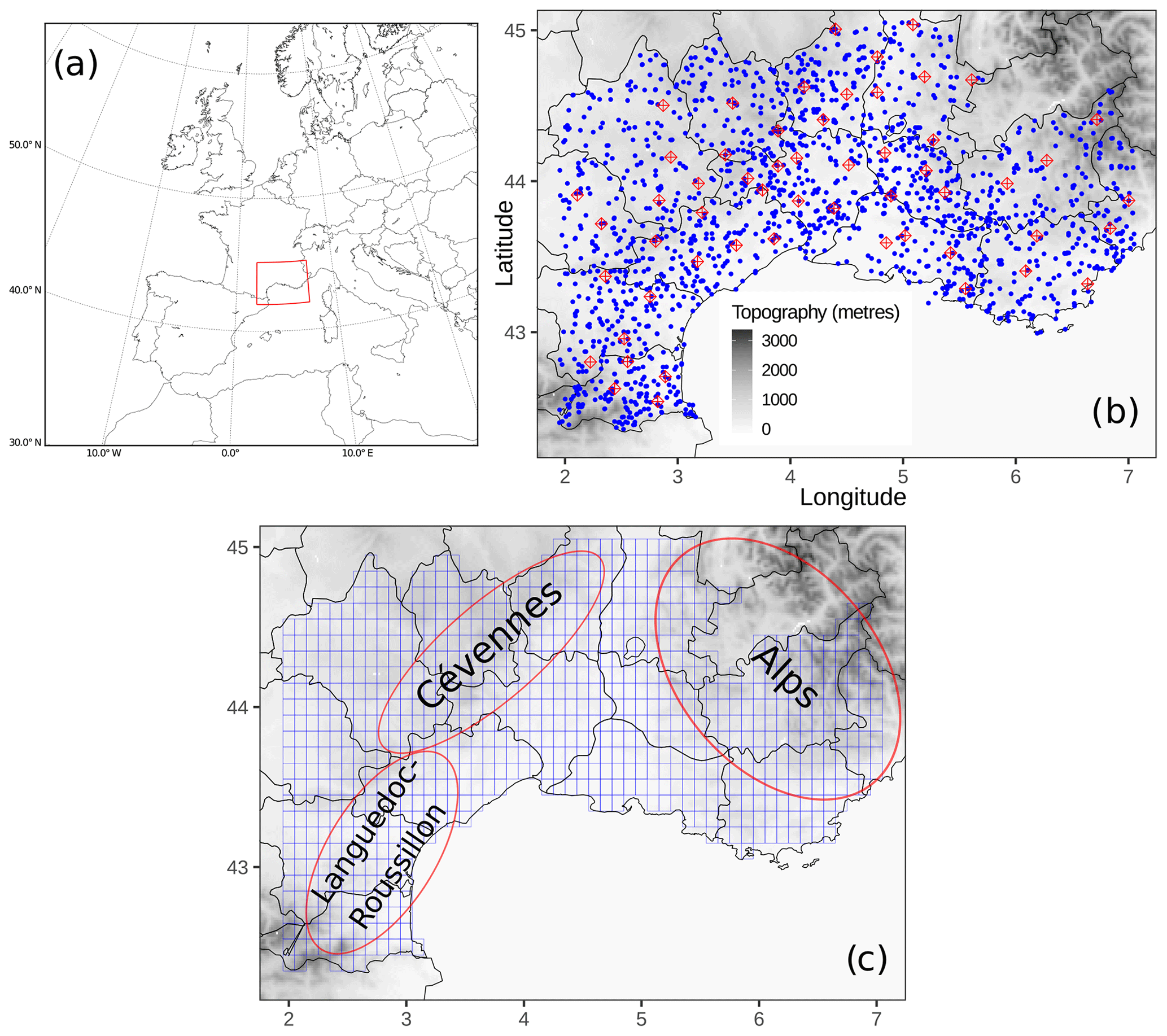
Figure 1 Panel (a) shows a situation map of the investigated area (rectangle with red edges) with respect to western Europe and the Mediterranean Sea. Panel (b) shows the rain-gauge network used for the study. Red diamonds represent the rain gauges selected for cross-validation testing, and blue dots represent the rain gauges selected for cross-validation training. Panel (c) shows the $\mathrm{0.1}{}^{\circ }\times \mathrm{0.1}{}^{\circ }$ model grid (in blue), along with the location of three key areas. Domain D is located within the borders of the model grid (c).

Table 1 Physical parameterizations used in the ensemble reforecast.

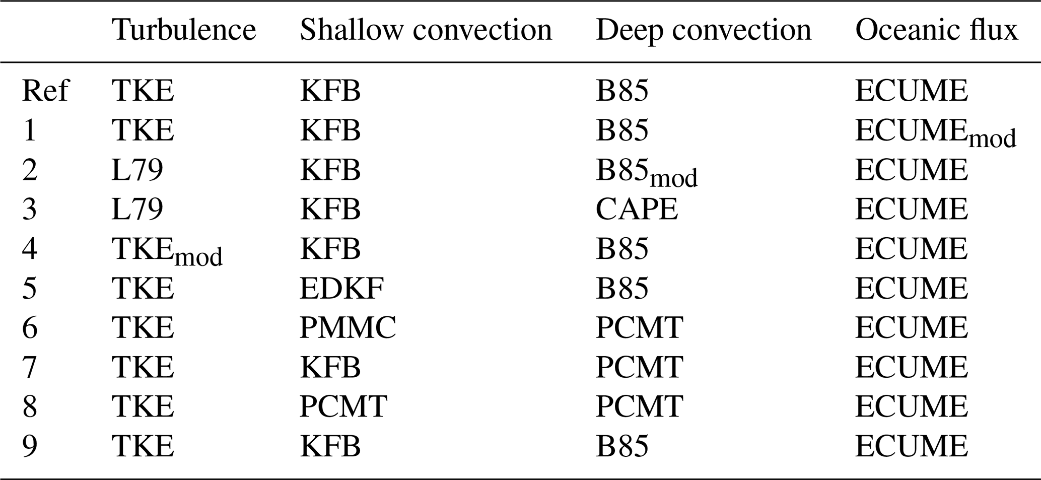
Nine different physical parameterizations (see Table 1) are added to the one that corresponds to the ARPEGE deterministic physical package. This set of parameterizations is the same as the one implemented in PEARP. Two turbulent diffusion schemes are considered: the turbulent kinetic energy scheme (TKE; Cuxart et al., 2000; Bazile et al., 2012) and the Louis scheme (L79; Louis, 1979). TKE_mod is a slightly modified version of TKE, in which horizontal advection is ignored. For shallow convection, different schemes are used: a mass flux scheme introduced by Kain and Fritsch (1993) and modified by Bechtold et al. (2001), hereafter called the KFB approach; the Prognostic Condensates Microphysics and Transport scheme (PCMT; Piriou et al., 2007); the eddy diffusivity and Kain–Fritsch scheme (EDKF); and the PMMC (Pergaud, Masson, Malardel, Couvreux) scheme (Pergaud et al., 2009). The deep-convection component is parameterized by either the PCMT scheme or the Bougeault (1985) scheme (hereafter B85). Closing the equation system used in these two schemes means relating the bulk mass flux to the in-cloud vertical velocity through a quantity γ qualifying the convection area coverage. Two closures are considered: the first one (C1) is based on the convergence of humidity, and the second one (C2) is based on the CAPE (convective available potential energy). The B85 scheme originally uses the C1 closure, while PCMT alternatively uses the closure (C1 or C2) which maximizes the γ parameter. Physics package 2 uses a modified version of the B85 scheme in which deep convection is triggered only if cloud top exceeds 3000 m (B85_mod in Table 1). The same trigger is used in physics package 3 in which deep convection is parameterized using the B85 scheme along with a CAPE closure (CAPE in Table 1). Finally the oceanic flux is solved by means of the ECUME (Exchange Coefficients from Unified Multicampaigns Estimates) scheme (Belamari, 2005). In ECUME_mod evaporation fluxes above sea surfaces are enhanced. Control member and member 9 are characterized by the same parametrization set-up, but member 9 differs for the modelling of orographic waves.

2.2 Daily rainfall reference

The 24 h accumulated precipitation is derived from the in situ Météo-France rain-gauge network, covering the same period as the reforecast dataset. The 24 h rainfall amounts collected from 14 French departments within the reforecast domain D are used (Fig. 1b). In order to maximize the rain-gauge network density within the region, all daily available validated data covering the period have been used.

Rain-gauge observations are used to build gridded precipitation references by a statistical spatial interpolation of the observations. The aim of this procedure is to ensure a spatial and temporal homogeneity of the reference, as well as the same spatial resolution as the reforecast dataset. Ly et al. (2013) provided a review of the different methods for spatial interpolation of rainfall data. They showed that kriging methods outperform deterministic methods for the computation of daily precipitation. However, both types of methods were found to be comparable in terms of hydrological modelling results. For the interpolation, we use a mixed geo-statistical and deterministic algorithm, which implements ordinary kriging (OK; Goovaerts, 1997) and inverse-distance-weighting methods (IDW; Shepard, 1968). For the kriging method, three semi-variogram models (exponential, Gaussian, and spherical) are fitted to a daily sample semi-variogram drawn from raw and square-root-transformed data (Gregoire et al., 2008; Erdin et al., 2012). This configuration involves the use of six different geo-statistical interpolation models. In addition, four different IDW versions are used, by varying the geometric form parameter d used for the estimation of the weights (see Eq. (2) in  Ly et al., 2011) and the maximum number n of neighbour stations involved in the IDW computation. Three versions are defined by fixing parameter d=2 and alternatively assigning n values equal to 5, 10, and N (with N being the total number of stations available for that specific day). In the fourth version we set n=N and d=3. For each day, a different interpolation method is used, and its selection is based on the application of a cross-validation approach. We select 55 rain gauges as a training dataset (see the red diamonds in Fig. 1c) in order to have sufficient coverage over the domain, especially on the mountainous area. Root-mean-square error (RMSE) is used as a criterion of evaluation. For each day, the method which minimizes the RMSE computed within the rain gauges of the training dataset is selected and the spatial interpolation is then performed on a regular high-resolution grid of 0.05^∘. The highest-resolution estimated points are then upscaled to the 0.1^∘ grid resolution of domain D, by means of a spatial average. This upscaling procedure aims at reproducing the filtering effect produced by the parameterizations of the model on the physical processes that occur below the grid resolution.

2.2.1 HPE database

We implement a methodology in order to select the HPEs from the daily rainfall reference. Anagnostopoulou and Tolika (2012) have examined parametric and non-parametric approaches for the selection of rare events sampled from a dataset. Here we adopt a non-parametric peak-over-threshold approach, on the basis of World Meteorological Organization (WMO) guidelines (World Meteorological Organization, 2016). The aim is to generate a set of events representative of the tail of the rainfall distribution for a given region and season. Following the recommendation of Schär et al. (2016), an all-day percentile ($P_{\mathrm{0}\le n\le \mathrm{1}}$) formulation is applied. A potential weakness of the research methodology based on the gridded observation reference is that a few extreme precipitation events affecting a smaller area than the grid resolution may not be identified. However, this approach has been preferred to a classification using rain gauges because spatial and temporal homogeneity are ensured.

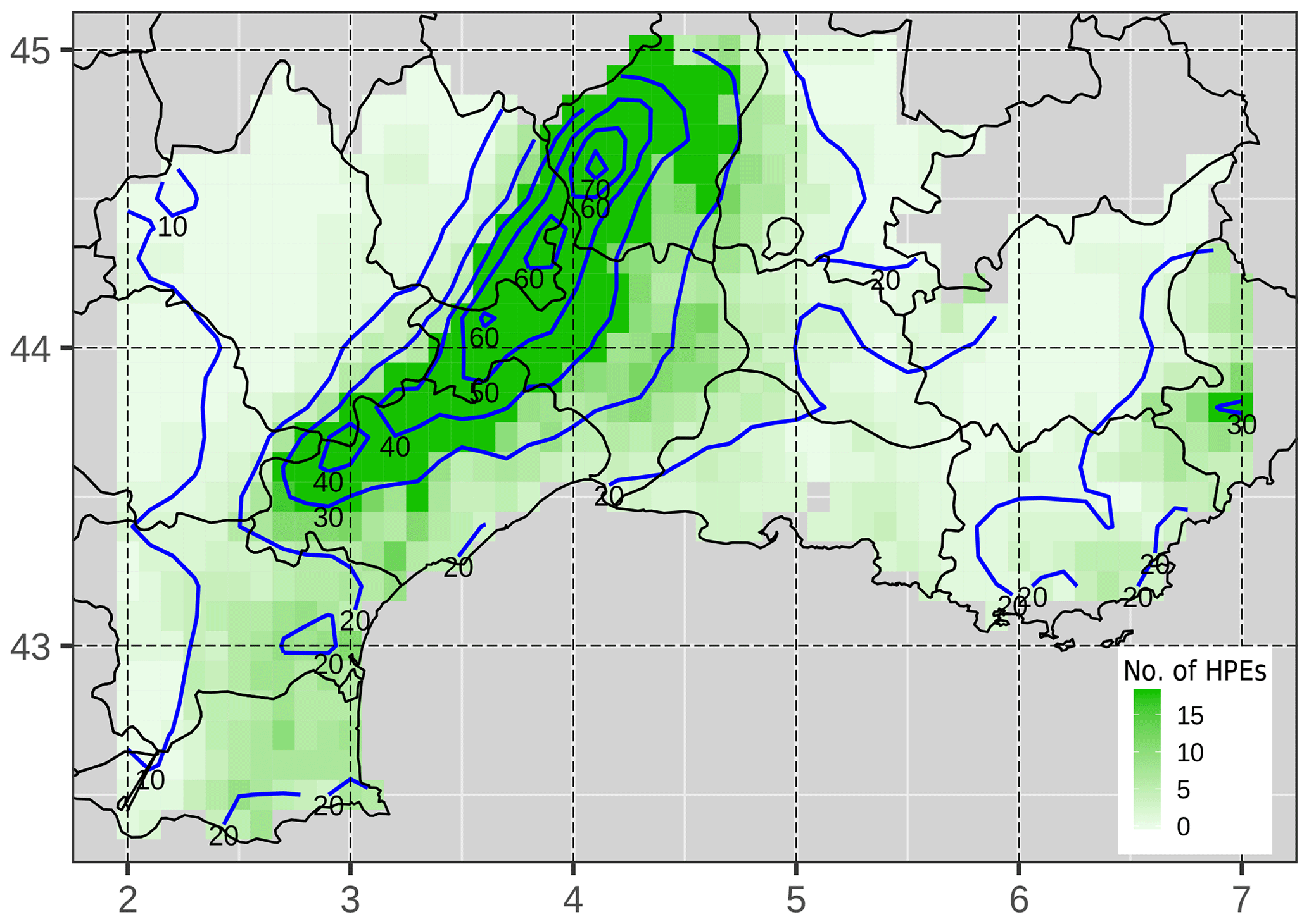
Figure 2 Annual average of HPE occurrence per grid point (in green). The composite of daily rainfall amounts (mm d⁻¹) of the HPE dataset is represented by the blue isohyets.

We proceed as follows: first the domain is split into two subregions based on the occurrence of climatological intense precipitation during the 30-year period. The subregion A includes all the points whose climatological percentile 99.5 is lower than or equal to a threshold T, and subregion B includes all the other points. Threshold T, after several tests, has been set to 85 mm. This choice was made in order to separate the domain into two regions characterized by different frequency and intensity of HPEs. Subregion A designates a geographical area where a large number of cases of intense precipitation are observed. Subregion B primarily covers the plain area, where HPE frequency is lower. For this reason, two different level threshold values are selected to define an event, depending on the subregion. More specifically, a day is classified as an HPE if one point of subregion A accumulated rainfall is greater than 100 mm or if one point of subregion B rainfall is greater than its percentile 99.5. The selection led to a classification of 192 HPEs, corresponding to a climatological frequency of 5 % over the 30-year period. The 24 h rainfall amount maxima within the HPE dataset range from 100 to 504 mm. It is worth mentioning that since we consider daily rainfall, rainfall events that would have high 48 h or 72 h accumulated rainfall may be disregarded. Figure 2 shows for each point of the domain the number of HPEs as well as the composite analysis of HPEs. The composite analysis involves computing the grid-point average from a collection of cases. The signal is enhanced along the Cévennes chain and in the Alpine region. It should be noted that some points are never taken into account for the HPE selection (white points of Fig. 2) because the required conditions have not been met. The analysis of the rainfall fields across the HPE database exhibits the presence of patterns of different shape and size, revealing potential differences in terms of the associated synoptic and mesoscale phenomena (not shown).

2.2.2 Clustering analysis

Clustering analysis methods can be applied to daily rainfall amounts in order to identify emergent regional rainfall patterns. This classification is largely used for assessing the between-day spatial classification of heavy rainfall (Romero et al., 1999; Peñarrocha et al., 2002; Little et al., 2008; Kai et al., 2011). We applied a cluster analysis, as an exploratory data analysis tool, in order to assess geographical properties of the precipitation reference dataset. The size of the dataset is first reduced, and the signal is filtered out by means of a principal component analysis (Morin et al., 1979; Mills, 1995; Teo et al., 2011). The first 13 principal components (PCs), whose projection explains 90 % of the variance, are retained. Then the K-means clustering method is applied. It is a non-hierarchical method based on the minimization of the intraclass variance and the maximization of the variance between each cluster. A characteristic of k-means method is that the number of clusters (K) into which the data will be grouped has to be a priori prescribed. Consequently, we first have to implement a methodology to find the number of clusters which leads to the most classifiable subsets.

Table 2 Classification of days computed from 24 h rainfall amounts in southern France (1981–2010), percentage of HPEs, and fraction of HPEs. HPEs (%) refers to the ratio between the number of HPEs within the cluster and the total number of HPEs. Fraction of HPEs (%) refers to the ratio between the number of HPEs within the cluster and the total number of dates included in the corresponding cluster.

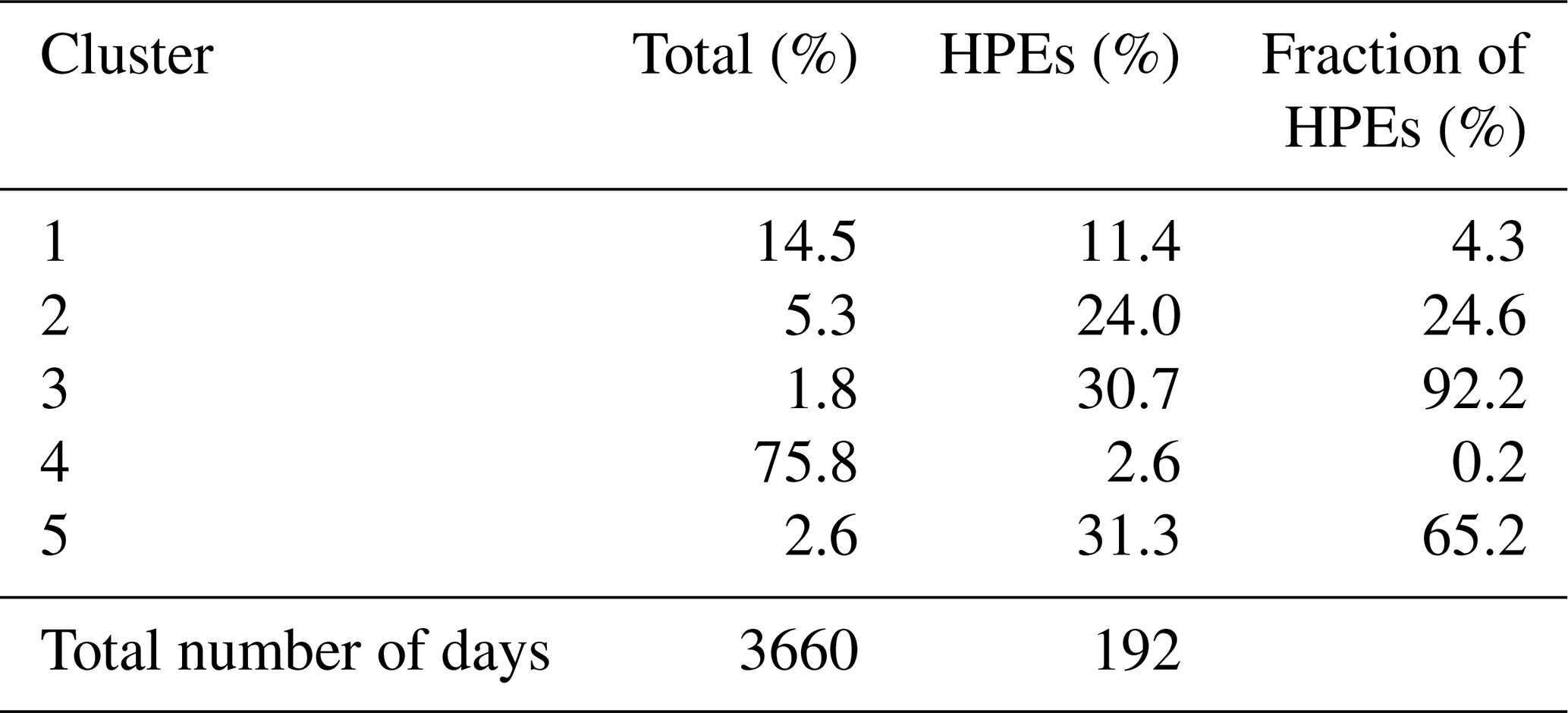
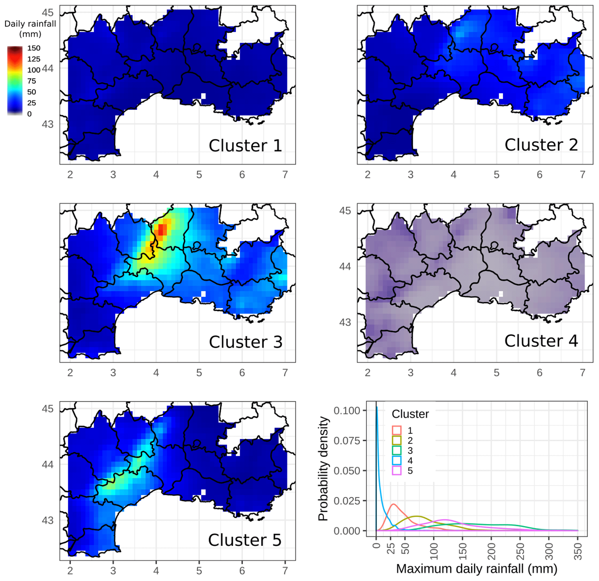
Figure 3 Rainfall composites (mm d⁻¹) for the five clusters selected by the K-means algorithm. The bottom right panel shows the probability density distribution of the maximum daily rainfall (mm) for each cluster class.

The analysis is applied to the full reference dataset, including rainy and dry days. We run 2000 tests for a range of a priori cluster numbers K that lies between 3 and 13, by varying a random initial guess each time. Then, for a given K, an evaluation of the stability of the assignment into each cluster is performed. The number of clusters is considered stable if each cluster size is almost constant from one test to another. K=5 is retained as the most stable number of clusters and because it suggests a coherent regional stratification of the daily rainfall data. The final classification within the 2000 tests is selected by minimizing the sum of the distance between the cluster centroids from each test and the geometric medians of cluster centroids computed from all the tests. The test which minimizes this quantity has been selected as the reference classification. The results from the cluster classification are summarized in Table 2. The clusterization shows large differences in terms of cluster size: more than three-fourths of the dataset is grouped in cluster 4, which mostly collects the days characterized by weak precipitation amounts or dry days. The percentage of HPEs within the clusters shows that the most intense events are represented in clusters 2, 3, and 5, among which cluster 5 shows the largest proportion of HPEs (65 % of HPEs within this cluster). Clusters 2, 3, and 5 together account for 86 % of the HPEs.

The same composite analysis as the one previously applied to HPE class is now computed for each cluster class (Fig. 3). It shows significant differences between clusters. The relative intensity of events and the location are different for each of the clusters. Rainfall range is weak for cluster 1 and close to zero for cluster 4. Cluster 2 includes some moderate 24 h rainfall amounts related to generalized precipitation events and a few HPEs. For cluster 1, composite values are slightly higher in the northwestern area of the domain, while for cluster 2 rainfall amount values are more significant on the eastern side of domain D. Clusters 3 and 5 together account for 63 % of the HPEs of the whole period, but rainfall events seem to affect different areas. Cluster 3 includes most of the events impacting the Cévennes mountains and the eastern departments on the southern side of the Alps. Cluster 5 average rainfall is enhanced along the southern side of the Cévennes, especially the Languedoc-Roussillon region.

The bottom right panel of Fig. 3 shows the density distributions computed from the maximum daily rainfall for each cluster. It is worth noting that cluster rainfall distributions cover different intervals of maximum daily rainfall amounts. Cluster 4 includes all the dry days. As this paper focuses on the most severe precipitation events, results will only be shown for clusters 2, 3, and 5 for the remainder of the paper.

2.3 The SAL verification score

2.3.1 The SAL score definition

The SAL score is an object-based quality measure introduced by Wernli et al. (2008) for the spatial verification of numerical weather prediction (NWP). It consists in computing three different components: structure S is a measure of volume and shape of the precipitation patterns, amplitude A is the normalized difference of the domain-averaged precipitation fields, and location L is the spatial displacement of patterns on the forecast/observation domains.

Different criteria for the identification of the precipitation objects could be implemented: a threshold level (Wernli et al., 2008, 2009), a convolution threshold (Davis et al., 2006a, b), or a threshold level conditioned to a cohesive minimum number of contiguous connected points (Nachamkin, 2009; Lack et al., 2010). The threshold level approach needs only one estimation parameter, so it has been preferred to the other methods for its simplicity and interpretability. Since we focus on the patterns associated with the HPEs, we decided to adapt the threshold definition given by $T_f=x_{max}\times f$, where x_max is the maximum precipitation value of the points belonging to the domain and f is a constant factor ($=\mathrm{1}/\mathrm{15}$, in the paper of Wernli et al., 2008). Here the coefficient f has been raised to one-fourth because a smaller value results in excessively large objects spreading out over most of domain D. Choosing a higher f factor enables us to obtain more realistic features within the domain considered. Threshold levels T_f are computed daily for the reforecast and the reference dataset. Although objects are smaller than the domain for most of the situations, a few objects extending outside the domain are consequently limited by the boundaries of the region concerned.

If we consider domain D, the amplitude A is computed as follows:

$$\begin{array}{}\text{(1)}& A={\displaystyle \frac{{〈R_{\mathrm{for}}〉}_{\mathrm{D}}-{〈R_{\mathrm{obs}}〉}_{\mathrm{D}}}{\mathrm{0.5}\left({〈R_{\mathrm{for}}〉}_{\mathrm{D}}+{〈R_{\mathrm{obs}}〉}_{\mathrm{D}}\right)}}\in \left[-\mathrm{2},\mathrm{2}\right],\end{array}$$

where _D denotes the average over domain D. R_for and R_obs are the 24 h rainfall amounts over D associated with the forecast and the observation, respectively. A perfect score is achieved for A=0. The domain-averaged rainfall field is overestimated by a factor of 3 if A=1. Similarly, it is underestimated by a factor of 3 if $A=-\mathrm{1}$. The amplitude is maximal (A=2) if $\frac{{〈R_{\mathrm{for}}〉}_{\mathrm{D}}}{{〈R_{\mathrm{obs}}〉}_{\mathrm{D}}}\to +\mathrm{\infty }$ and minimal ($A=-\mathrm{2}$) if $\frac{{〈R_{\mathrm{for}}〉}_{\mathrm{D}}}{{〈R_{\mathrm{obs}}〉}_{\mathrm{D}}}\to \mathrm{0}$.

The two other components require the definition of precipitation objects (thereafter {Obj}), also called features, which represent contiguous grid points belonging to domain D, characterized by rainfall values exceeding a given threshold. The location L is a combined score defined by the sum of two contributions, L1 and L2. L1 measures the magnitude of the shift between the centre of mass of the whole precipitation field for the forecast (${\overline{x}}_{\mathrm{for}}$) and observation (${\overline{x}}_{\mathrm{obs}}$):

$$\begin{array}{}\text{(2)}& L\mathrm{1}={\displaystyle \frac{\mathrm{|}{\overline{x}}_{\mathrm{for}}-{\overline{x}}_{\mathrm{obs}}\mathrm{|}}{d}}\in \left[\mathrm{0},\mathrm{1}\right],\end{array}$$

where d is the largest distance between two boundary points of the considered domain D. The second metric L2 takes into account the spatial distribution of the features inside the domain, that is, the scattering of the objects:

$$\begin{array}{}\text{(3)}& r={\displaystyle \frac{{\sum }_{n=\mathrm{1}}^N{M}_n\mathrm{|}\overline{x}-x_n\mathrm{|}}{{\sum }_{n=\mathrm{1}}^N{M}_n}},\end{array}$$

where M_n is the integrated mass of the object n, x_n is the centre of mass of the object n, N is the number of objects, and $\overline{x}$ is the centre of mass of the whole field.

$$\begin{array}{}\text{(4)}& {\displaystyle }L\mathrm{2}=\mathrm{2}{\displaystyle \frac{\mathrm{|}{r}_{\mathrm{for}}-r_{\mathrm{obs}}\mathrm{|}}{d}}\in \left[\mathrm{0},\mathrm{1}\right]\text{(5)}& {\displaystyle }L=L\mathrm{1}+L\mathrm{2}\in \left[\mathrm{0},\mathrm{2}\right]\end{array}$$

L2 aims at depicting object differences between observed and forecasted scattering of the precipitation objects. We can notice that the scattering variable (Eq. 3) is computed as the weighted distance between the centre of total mass and the centre of mass of each object. Therefore L is a combination of the information provided by the global spatial distribution of the fields (L1) and the difference in scattering of the features over the domain (L2). The location score is perfect if $L\mathrm{1}=L\mathrm{2}=\mathrm{0}$, so if L=0 all the centres of mass match each other.

The S component is based on the computation of the integrated mass M_k of one object k, scaled by the maximum rainfall amount of the object k:

$$\begin{array}{}\text{(6)}& V_k={\displaystyle \frac{M_k}{maxR(x;x\in {\mathrm{Obj}}_k)}}.\end{array}$$

Then, the weighted average V of all features is computed, in order to obtain a scaled, weighted total mass:

$$\begin{array}{}\text{(7)}& {\displaystyle }V={\displaystyle \frac{{\sum }_{n=\mathrm{1}}^N{M}_n{V}_n}{{\sum }_{n=\mathrm{1}}^N{M}_n}},\text{(8)}& {\displaystyle }S={\displaystyle \frac{V_{\mathrm{for}}-V_{\mathrm{obs}}}{\mathrm{0.5}(V_{\mathrm{for}}+V_{\mathrm{obs}})}}\in \left[-\mathrm{2},\mathrm{2}\right].\end{array}$$

Then, S represents the difference of both forecasted and observed volumes, scaled by their half-sum. It is important to scale the volume so that the structure is less sensitive to the mass, meaning that it relates more to the shape and extension of the features rather than their intensities. In particular S<0 means that the forecast objects are large and/or flat compared to the observations. Inversely, peaked and/or smaller objects in the forecast give positive values of S. We refer to Wernli et al. (2008) for the exploration of the behaviour of SAL for some idealized examples.

On the basis of the definition of the score, it can be noticed that A and L1 components are not affected by the object identification and depend only on the total rainfall fields.

2.3.2 A selected example of the application of SAL

An example of the SAL score applied to an HPE, which occurred on 28 October 2004, is shown in Fig. 4 (60 h lead time forecast run using the physical package n.8). For the rainfall reference, a 24 h rainfall maximum value (121.3 mm) was registered in the southeastern coastal region. Therefore the threshold level T_f is set to 30.3 mm. For the forecast, the maximum value is 123.1 mm (T_f=30.8 mm), and, in contrast with the reference, it is located in Cévennes. The number of objects, three, is equivalent in both fields. The value of A is 0.08, which means that the domain-averaged precipitation field of the forecast is nearly similar to the reference one. The structure S component is positive (0.28), which could be explained by the larger forecast object over the Cévennes area, while the object along the southeastern coast is smaller and less intense. The contribution of the third object is negligible for the computation of S. The L component is equal to 0.23, with L1=0.13 and L2=0.10. The location error L1 means that the distance between the centres of total mass (see diamonds in Fig. 4) is 13∕100 of the largest distance between two boundary points of the considered domain. This error is mostly due to the fact that the most intense rainfall patterns are far apart from each other in the observations and the forecast.

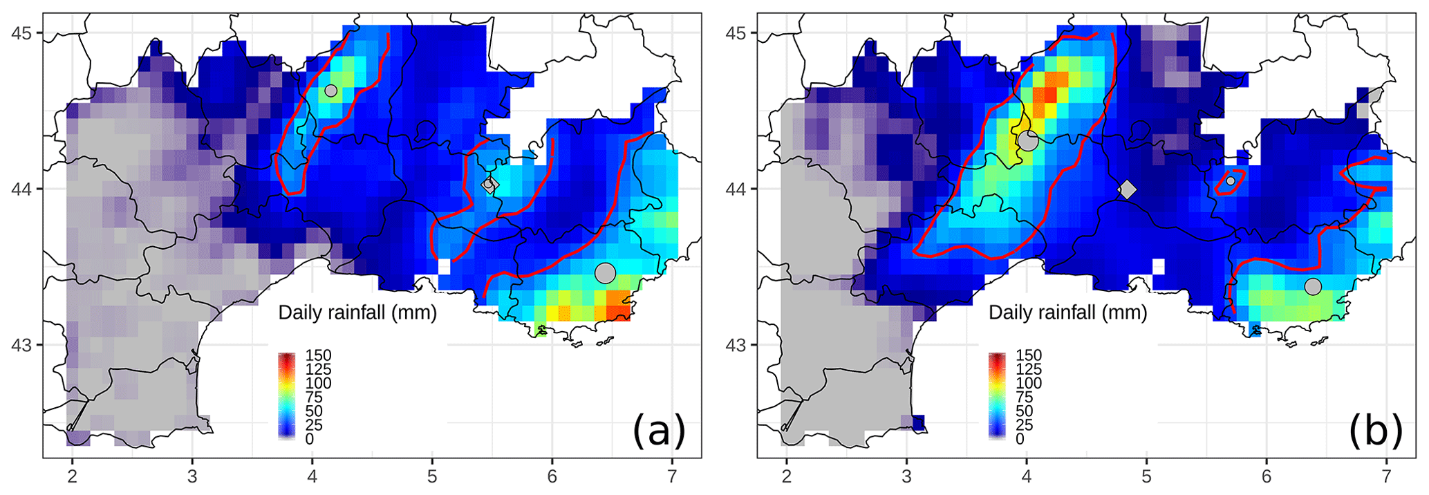
Figure 4 SAL pattern analysis for the case of 28 October 2004, applied to the observation data (a) and one 60 h lead time forecast (b). Base contours of the identified objects are shown as red lines. Grey points stand for the rain barycentre of each pattern, and the grey diamond depicts the rain barycentre for the whole field. The size of the barycentre points is proportional to the integrated mass of the associated object.

3 Analysis of the reforecast HPE representation

An SAL verification score has been applied to the reforecast dataset to perform statistical analysis of QPF (quantitative precipitation forecast) errors. The reforecast dataset is considered to be a test-bed model in order to study sources of systematic errors in the forecast. The overall reforecast performance is first examined for HPEs and non-HPEs, then according to the clusters. In a second step, the behaviour of the different physics schemes is analysed by separately considering the SAL results of each reforecast member. Similarly, the analysis is again allocated to HPEs and non-HPEs and subsequently to each cluster.

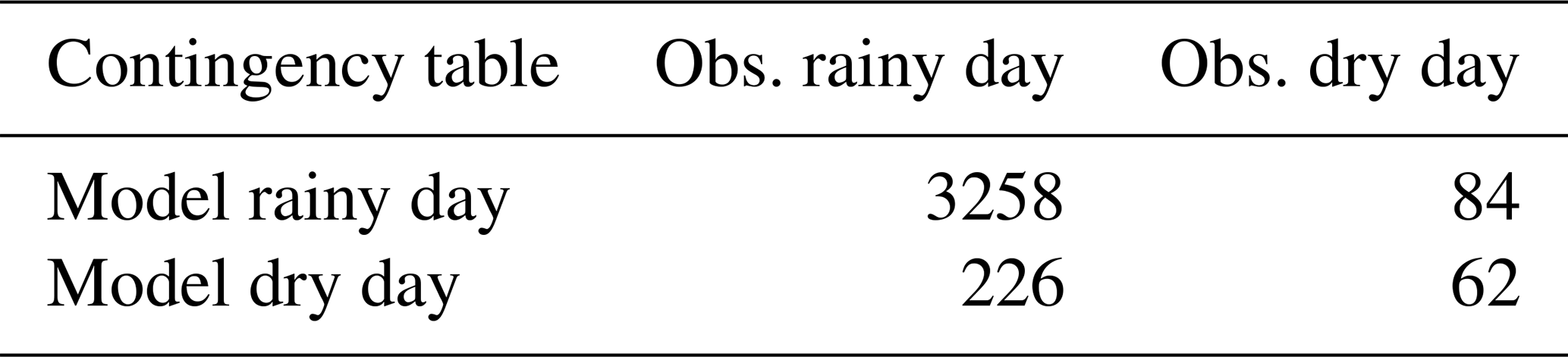
For both the reforecast and the reference, we set all the days with at least one grid point beyond 0.1 mm as a rainy day. In order to facilitate the comparison between the parameterizations, SAL verification is only performed when all the members and the reference are classified as rainy days. Table 3 shows the contingency table of the rainy and dry days. Therefore 84 false alarms, 226 missed cases, and 62 correctly forecast dry days are not involved in the SAL analysis. No HPEs belong to the misses, and no simulated HPEs belong to the false alarms. The SAL measure is then applied to the 3258 rainy days.

Table 3 Contingency table computed for rainy and dry days.

3.1 SAL evaluation of the HPE forecast

3.1.1 HPEs and non-HPEs

First the relationship between the A component of SAL and the maximum grid-point error is investigated (Fig. 5). The 36 and 60 h lead times (LT12 hereafter) and 84 and 108 h lead times (LT34 hereafter) are grouped together. Maximum daily absolute errors range between −250 and 250 mm. Rare higher values are observed, which are likely related to strong double-penalty effects that often occur in grid-point-to-grid-point verification. Points are mostly scattered along the amplitude axis, showing that the error dependence on the A component is weak. Concerning HPEs, the scatter plot shows A component values under 1, which means that the scaled average precipitation in the forecast never exceeds 3 times the observation. In contrast, A-component negative values are predominant, in particular at LT34, in relation to strong underestimations of the domain-averaged rainfall field. Some cases of significant maximum grid-point errors in conjunction with a moderate negative A component must be related to strong location errors. In these cases, the domain-averaged field may be similar to the observed one while the maximum rainfall is spatially deviated. For the non-HPEs, we can see that, especially for LT34, the model could significantly overestimate both the A component and the maximum grid-point error.

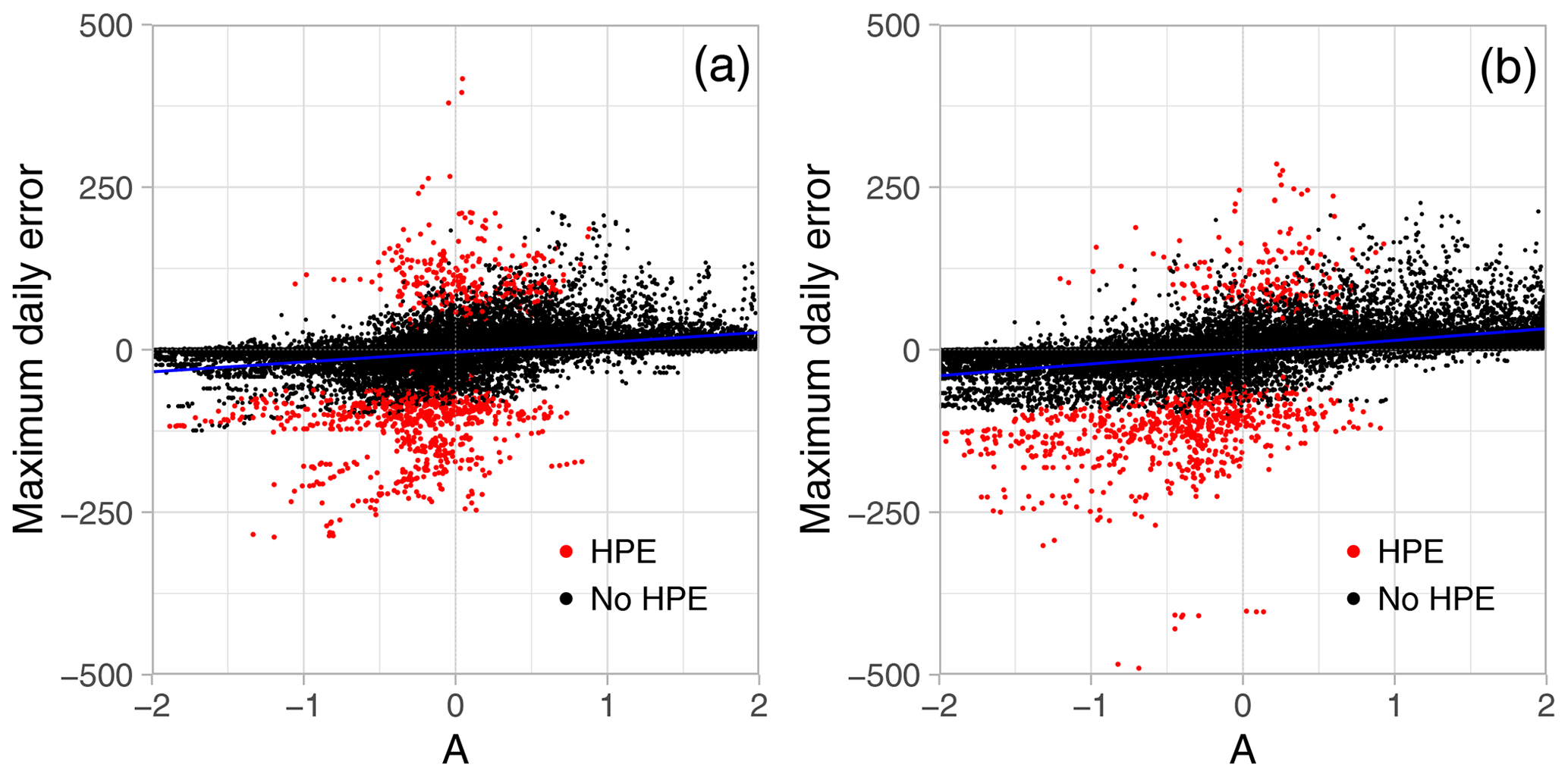
Figure 5 Relationship between the daily rainfall grid-point maximum algebraic error and the A component of the SAL score. HPE days are plotted in red, while other days are in black. Panel (a) is for LT12 lead time, and (b) shows LT34 lead time. Linear regression analysis is added to the plot.

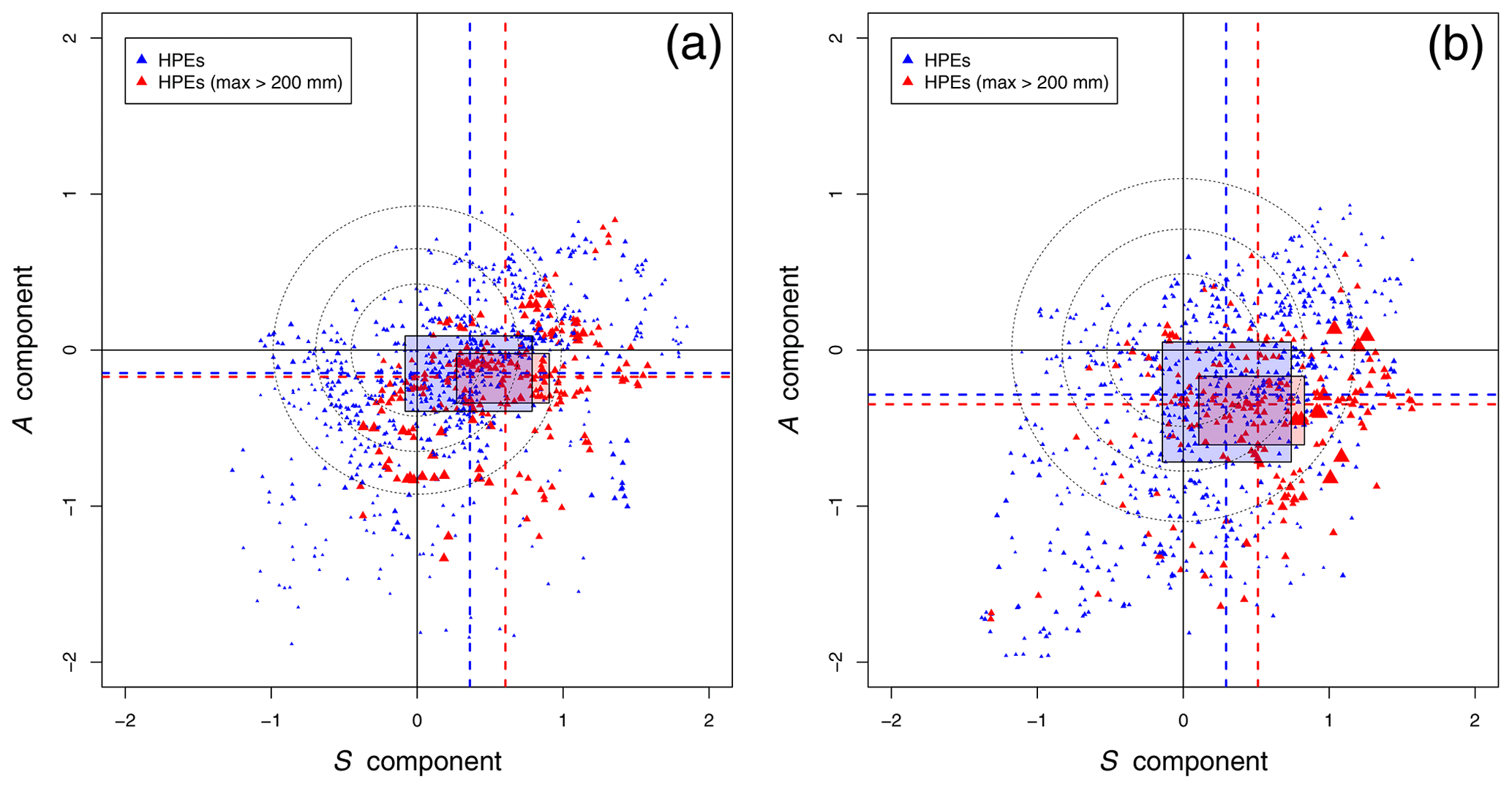
Figure 6 Relationship between the A component and the S component of the SAL score (SAL diagrams) for HPEs only, for lead times LT12 (a) and LT34 (b). Blue triangles represent HPEs with grid-point maximum rainfall under 200 mm d⁻¹, and red triangles show rainfall amounts above 200 mm. Triangles are proportional to the rainfall value. Some main characteristics of the component distribution are plotted. The median value is shown as dashed lines, and percentiles 25 and 75 delimitate the boxes. Circles represent the limits 25th, 50th, and 75th percentiles to the best score (A=0, S=0).

The relationship between the different SAL components might help to understand sources of model error. In Fig. 6 the S and A components are drawn for the HPEs only. Perfect scores are reached for the points located on the origin O of the diagram. Very few points are located in the top left-hand quadrant. This indicates that an overestimation of precipitation amplitude associated with too small rainfall objects is rarely observed. The points, especially for LT34, are globally oriented from the bottom left-hand corner to the top right-hand corner. This suggests a linear growth of the A component as a function of the S component, which means that the average rainfall amount is roughly related to the structure of the spatial extension. For the two diagrams, it can also be noticed that many of the points are situated in the lower right quadrant, suggesting the presence of too large and/or flat rainfall objects compared to the reference while the corresponding A component is negative. This is supported by the values of the medians of the distribution of the two components (dashed lines) and the quartile values (respective limits of the boxes). The positive bias in the S component is even stronger for the most extreme HPEs (red triangles). The distortion of S-component error compared to the A component shows that the model has more difficulties reproducing the complex spatial structure than simulating the average volume of a heavy rainfall. This deficiency may be related to the convection part not represented in the parametrization scheme. It may also be related to the representation of orography at a coarse resolution. As shown by Ehmele et al. (2015), an adequate representation of topographic features and local dynamic effects is required to correctly describe the interaction between orography and atmospheric processes. Furthermore, initial conditions have been shown to have a significant influence on rainfall forecasting (Kunz et al., 2018; Khodayar et al., 2018; Caldas-Álvarez et al., 2017).

For each point of the diagram in Fig. 6, we compute its distance from the origin (perfect score – A=0, S=0). The dotted circles respectively contain the 25 %, 50 %, and 75 % points with the smallest distance. The radii of the circles are much larger for LT34, confirming a degradation of the scores for longer lead times.

3.1.2 Clusters

We use our clustering procedure (as defined in Sect. 2.2.2) to analyse the characteristics of the forecast QPF errors along with the regional properties. SAL components are stated for each day of each cluster associated with HPEs, i.e. C2, C3, and C5. In Fig. 7, PDFs (probability density functions) are drawn from the corresponding normalized histograms for the two lead times LT12 and LT34. The distributions of the A component are negatively skewed for all the clusters. This shows that the model tends to produce too weak domain-averaged rainfall in the case of heavy rainfall. This is even more important for clusters 3 and 5. For long lead times, the distributions are flatter, showing that the left tail of the A-component PDF spreads far away from the perfect score.

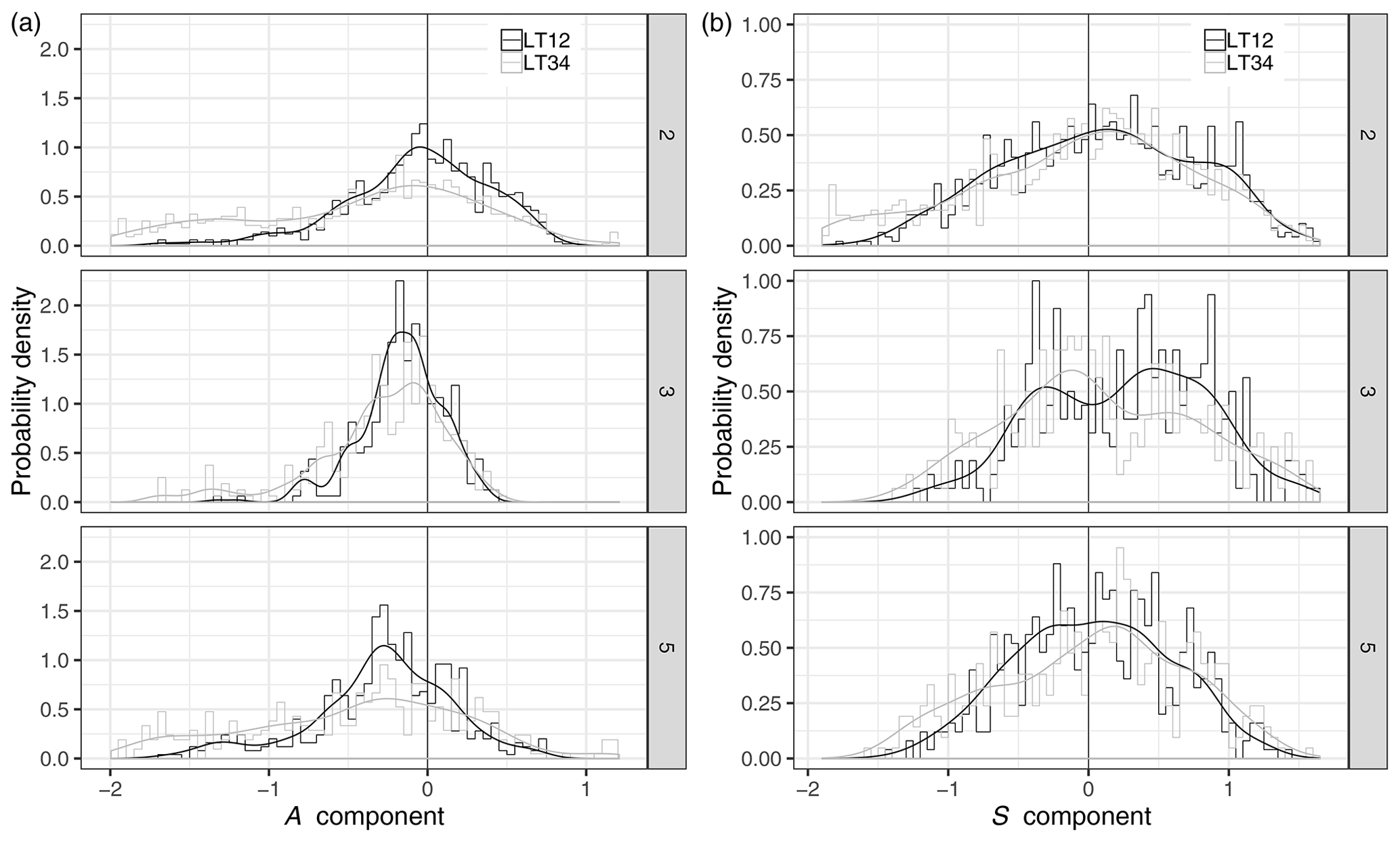
Figure 7 A-component (a) and S-component (b) normalized histograms and probability density functions for clusters 2, 3, and 5. Results for lead time LT12 are plotted as black lines, and results for lead times LT34 are in grey.

Table 4 Pearson correlation between the daily mean S component and the maximum daily rainfall for the three cluster classifications. A t test is applied to the individual correlations. For the three clusters, the null hypothesis (true correlation coefficient is equal to zero) is rejected.

The distributions of the S component (right panels) are positively skewed in clusters 2 and 3, while they are more centred for cluster 5. For all the clusters, the spread of the S-component distributions is less dependent on the lead time, compared to the A-component distributions. It is interesting to examine whether a relationship between the S component and the intensity of the rainfall can be identified. A Pearson correlation coefficient is computed between the daily mean of the S component estimated within the 10 members of the reforecast and the maximum observed daily rainfall for each cluster class (Table 4). A positive correlation is found for all three clusters, which corroborates the results from Fig. 6 where HPEs correspond to the highest S-component values. The maximum correlation is found for cluster 3. Although correlations are statistically significant, it is worth noting that values are quite weak (in particular for cluster 5).

3.2 Sensitivity to physical parameterizations

The SAL measure is analysed separately for the 10 different physical packages to study corresponding systematic errors. More specifically, we raise the following questions. Do the errors based on an object-quality measure and computed for the different physics implemented in an ensemble system show different rainfall structure properties? Which physical packages are more sensitive to the intense rainfall forecast errors? As in Sect. 3.1, we first distinguish the results for the HPE group before the cluster ones.

3.2.1 HPEs

Probability density distributions for each SAL component are separately computed for each physics reforecast (Fig. 8), considering only the HPEs. Colours correspond to four categories, depending on the parametrization of the deep convection. The figure highlights that members from each of the two main parametrization schemes (B85 and PCMT) have similar behaviours. Considering the A component, PCMT members are more centred around zero than B85 at LT12. This effect is higher at LT34, for which B85 and PCMT density distributions are more shifted. At LT34, more events with a positive A component are associated with PCMT, whereas negative values are more recurrent in B85. The A component never exceeds +1, but significant underestimations are observed. This range of values stems from the fact that the forecast verification is applied to a subsample of the observation limited to the most extreme events. For these specific events, a model underestimation is more frequent than an overestimation. At short lead times, the separation between the two deep-convection schemes is also well established for the S component (Fig. 8), but it becomes mixed up at LT34 (Fig. 8). One reason for this behaviour could be that predictability decreases at LT34, so that discrepancies in spatial rainfall structure assigned to the physics families become less identifiable. The S component is positively skewed in all cases (in particular for the B85 physics at LT12 lead time). This supports the previous analysis of the S component (Figs. 6 and 7), showing that for intense rainfall the model mostly produces a larger and flatter rainfall signal. The results for the S component also highlight better skills for PCMT schemes for HPEs, especially at short lead times. Focusing on high values of S, B85 exhibits a stronger distribution tail at LT12, while both schemes seem comparable for LT34.

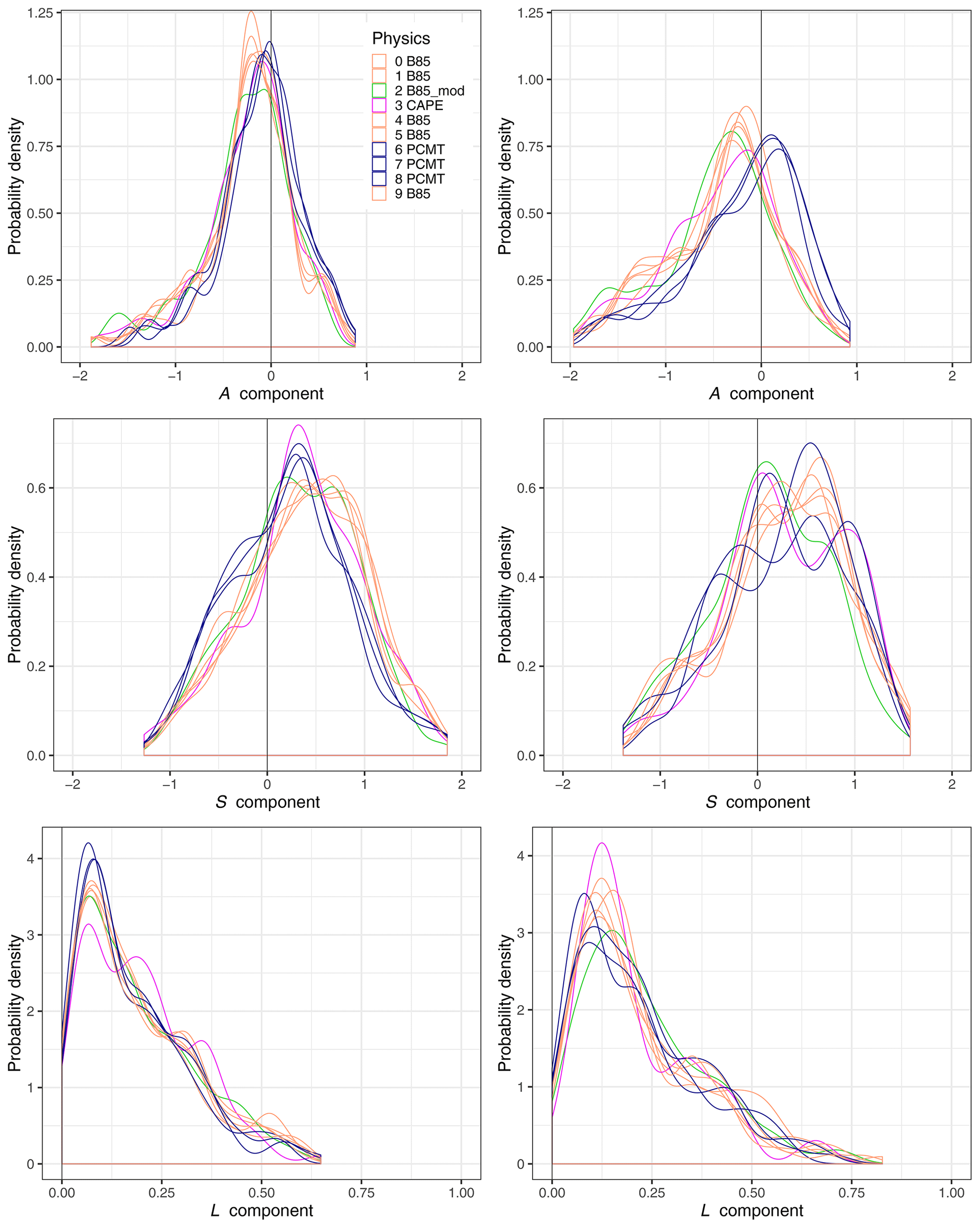
Figure 8 Probability density functions of the three SAL components for the HPEs and for each physics of the reforecast system (coloured lines). Physics scheme are gathered in four categories depending on the parametrization of the deep convection: PCMT (blue), B85 (orange), B85_mod (green), and CAPE (purple). The left column corresponds to lead time LT12, and the right column relates to lead time LT34.

For the L component, the maxima of the density distributions are higher for PCMT at lead time LT12, implying a more significant number of good estimations of pattern location. Regarding the tail of the L-component PDF, it is globally more pronounced at LT34 than LT12. This means that the location of HPEs is poorly forecasted at long lead times. Concerning the behaviour of the forecasts that use the CAPE or B85_mod schemes, their A-component PDFs are close to the B85 PDFs. This is not observed for the other components. For the S component, the CAPE distribution follows the PCMT one at LT12. For the L component, the B85_mod PDF is close to the B85 ones, while CAPE shows different behaviour from all the other physics. The use of a closure based on CAPE, rather than on the convergence of humidity, seems to modulate the location of precipitation produced by this deep-convection parametrization scheme. Moreover, at LT34 CAPE is characterized by a lower number of strong location errors, compared to the other physics.

3.2.2 Clusters

According to the results of the previous section, which show that the predictability of intense rainfall events is sensitive to the parametrization of the deep convection, we have continued to analyse the model behaviour for the four different deep-convection schemes: B85, B85_mod, CAPE, and PCMT. The link between the behaviour of the physical schemes and belonging to a particular cluster is statistically assessed through the SAL component differences between the schemes.

Any parametric goodness-of-fit tests, which assume normality, have been discarded, because SAL values are not normally distributed. We choose the k-sample Anderson–Darling (AD) test (Scholz and Stephens, 1987; Mittermaier et al., 2015), in order to evaluate whether differences between two given distributions are statistically significant. It is an extension of the two-sample test (Darling, 1957), originally developed starting from the classic Anderson–Darling test (Anderson and Darling, 1952). The k-sample AD test is a non-parametric test designed to compare continuous or discrete subsamples of the same distribution. In this case the test is implemented for the evaluation of the pairs of distributions.

The tests are performed for the comparison of each pair of PDFs combined from the four deep-convection families and from the three clusters' classification. For the A component, PCMT physics distributions depart significantly from B85 schemes at all lead times, while B85_mod and CAPE perform as B85, meaning that the modified versions of B85 weakly affect physics behaviour (not shown).

With respect to the S-component distributions, k-sample AD tests show significant differences between B85 and PCMT physics for LT12, but not for the longest lead times (not shown). At LT34 we observe a convergence of the physics scheme towards a homogeneous distribution, meaning that the differences between physics are negligible.

The test applied to the location component does not reveal significant differences between the PDFs. We suppose that the limited dimensions of the domain employed in this study, as well as its irregular shape, may lead to a less coherent estimation of the location, resulting in a degradation of the score significance. Since the L-component result is not informative about HPEs, it is ignored hereafter.

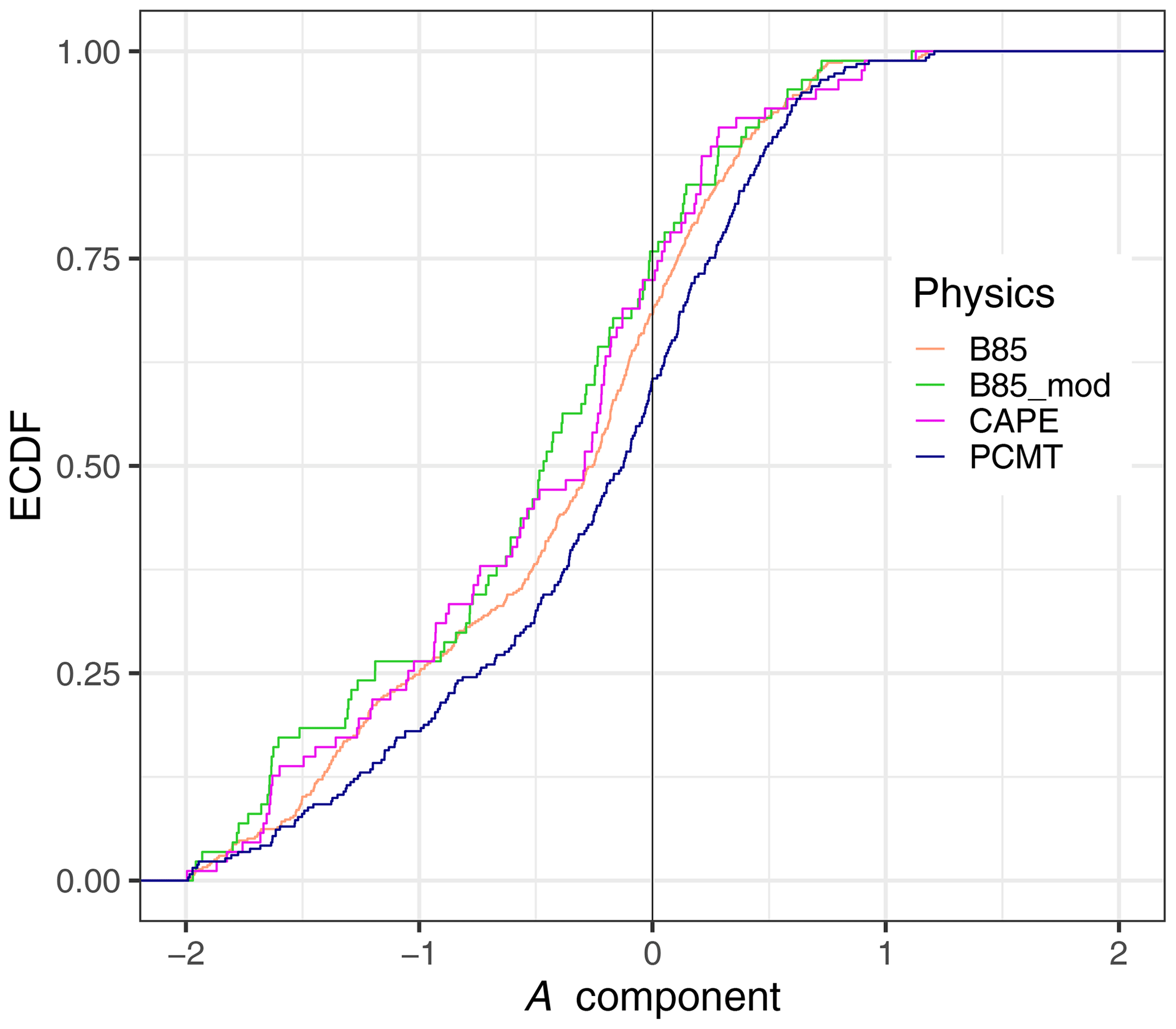
Figure 9 Empirical cumulative distribution function of the A component computed from cluster 2 at lead time LT34 for the four classes of physics schemes.

Once the statistical differences between the PDFs of the physics have been examined, it is interesting to compare the relative error on the amplitude and structure components. S and A component errors are estimated by comparing the shapes of their distributions. Empirical cumulative density functions (ECDFs) of S and A components are computed separately for each cluster and lead time (LT12 and LT34). We show an example of an ECDF for cluster 2 at LT34 (Fig. 9). Forecasts are perfect when the ECDF tends towards a Heaviside step function, which means that the distribution tends towards the Dirac delta function centred on zero. These functions are estimated over a bounded interval, corresponding to the finite range of S and A components. The deviation from the perfect score was quantified by estimating the area under the ECDF curve on the left side and the area above the ECDF curve on the right side:

$$\begin{array}{}\text{(9)}& {\displaystyle }\begin{array}{rl}{\mathrm{err}}_{-}& =\underset{-\mathrm{2}}{\overset{\mathrm{0}}{\int }}F\left(x\right)\mathrm{d}x-\underset{-\mathrm{2}}{\overset{\mathrm{0}}{\int }}H\left(x\right)\mathrm{d}x=\underset{-\mathrm{2}}{\overset{\mathrm{0}}{\int }}F\left(x\right)\mathrm{d}x-\mathrm{0}\\ & =\underset{-\mathrm{2}}{\overset{\mathrm{0}}{\int }}F\left(x\right)\mathrm{d}x,\end{array}\text{(10)}& {\displaystyle }{\mathrm{err}}_{+}=\underset{\mathrm{0}}{\overset{\mathrm{2}}{\int }}H\left(x\right)\mathrm{d}x-\underset{\mathrm{0}}{\overset{\mathrm{2}}{\int }}F\left(x\right)\mathrm{d}x=\mathrm{2}-\underset{\mathrm{0}}{\overset{\mathrm{2}}{\int }}F\left(x\right)\mathrm{d}x,\text{(11)}& {\displaystyle }\mathrm{err}={\mathrm{err}}_{-}+{\mathrm{err}}_{+}=\mathrm{2}-\underset{\mathrm{0}}{\overset{\mathrm{2}}{\int }}F\left(x\right)\mathrm{d}x+\underset{-\mathrm{2}}{\overset{\mathrm{0}}{\int }}F\left(x\right)\mathrm{d}x,\end{array}$$

where F(x) is the ECDF computed for A or S, H(x) is the Heaviside step function, and err is the forecast error for a given component. The lower and upper boundaries of the integrals are equal to −2 and +2, because A and S components range between these two values by construction. Since the previous k-sample AD test highlighted significant differences within the two main classes B85 and PCMT, the evaluation of the errors is limited to these two specific classes.

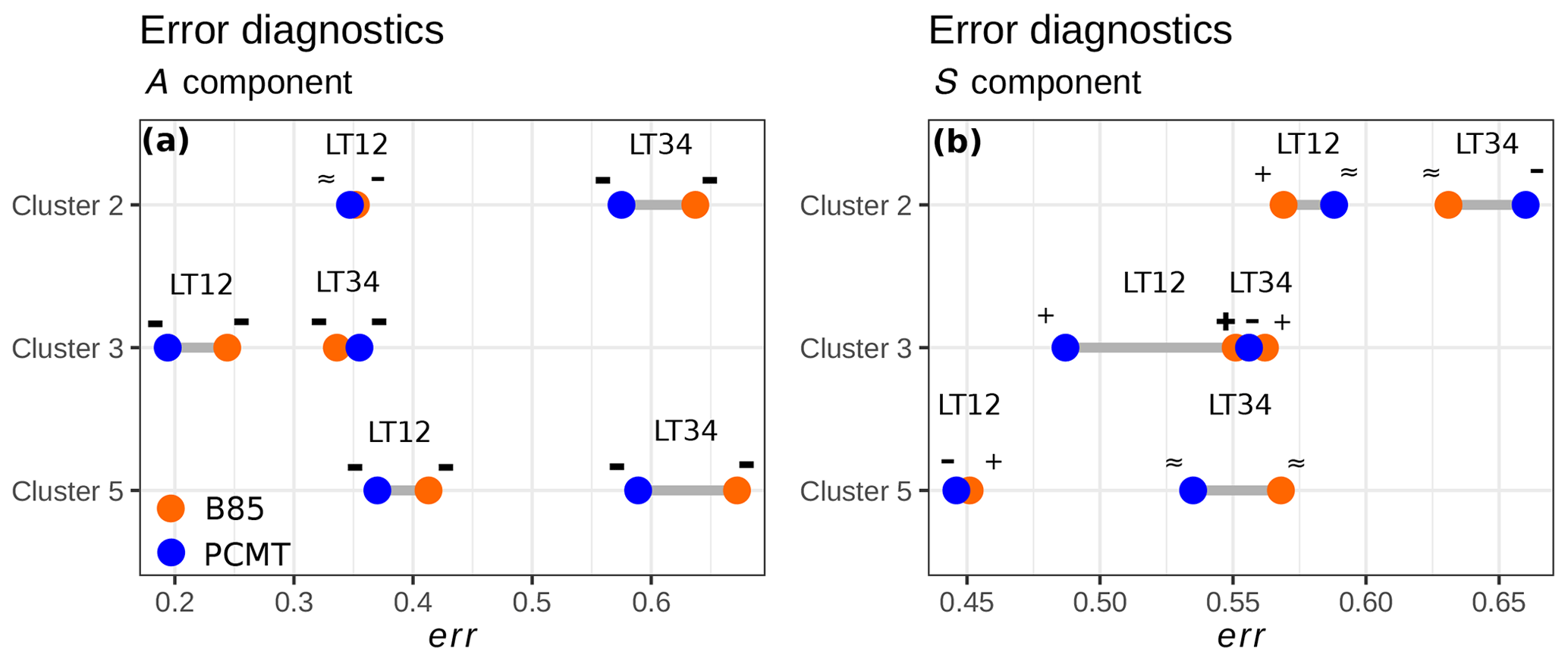
Figure 10 Dumbbell plot of integrated error diagnostics computed using Eq. (11). Colours refer to B85 (orange) and PCMT (blue) deep-convection parametrization schemes. Results are stratified on the basis of the clusters and lead times. Symbols denote whether positive or negative errors dominate. These signs are defined using the following definition: - (bold) if $\frac{{\mathrm{err}}_{-}}{{\mathrm{err}}_{+}}\ge \mathrm{2}$; − if $\mathrm{1.1}\le \frac{{\mathrm{err}}_{-}}{{\mathrm{err}}_{+}}<\mathrm{2}$; ≈ if $\mathrm{0.9}<\frac{{\mathrm{err}}_{-}}{{\mathrm{err}}_{+}}<\mathrm{1.1}$; + if $\mathrm{0.5}<\frac{{\mathrm{err}}_{-}}{{\mathrm{err}}_{+}}\le \mathrm{0.9}$; + (bold) if $\frac{{\mathrm{err}}_{-}}{{\mathrm{err}}_{+}}\le \mathrm{0.5}$.

The results of the error diagnostic err for the A component are shown in Fig. 10a. Errors increase with lead time. We note that the negative errors are always at least twice as large as the positive ones. Forecasted averaged rainfall amounts are almost always underestimated. PCMT produces overall better A-component statistics, except for cluster 3 at LT34. It is interesting to observe that the weakest errors are associated with cluster 3, which is the most extreme one. Since cluster 3 collects a large number of precipitation events impacting the Cévennes chain, we may suppose that the domain-averaged rainfall amounts are more predictable in situations of precipitation driven by the orography. Concerning the S-component evaluation (see Fig. 10b), structures of rainfall patterns are better forecasted for heavy-rainfall events (clusters 3 and 5) than for the remaining classes of events. In contrast to the A component, the S component exhibits the highest err₊ for the B85 scheme for most of the cases (majority of + signs in Fig. 10b), whereas this trend is not systematic for PCMT physics. PCMT globally performs better than B85, except for cluster 2. As with the amplitude A, the S component gets worse for longer lead times, resulting in a shift to larger err₋ for both B85 and PCMT physics (more – sign for LT34 in Fig. 10a, b). The lowest errors of the S component are achieved for cluster 5. Cluster 5 HPEs are known to have specific regional properties whose influence on S-component results should be studied with further diagnostics.

3.2.3 Rainfall object analysis

We now analyse the physical properties of the objects, i.e. the number of objects from a rainfall field and the object-integrated volumes, according to the different clusters. All the statistics are applied separately to the B85, PCMT physics, and observations. For each day of the dataset period, the thresholds defined in Sect. 2.3.1 lead to the identification of a certain number of precipitating objects. The frequency of the number of objects per day is plotted by means of normalized histograms for the three clusters (Fig. 11). Clusters 2 and 3 show maximum frequency for one- and three-object ranges, whereas cluster 5 is dominated by one object per day. This specific property of cluster 5 can explain the best result obtained for the S component (Sect. 3.2.2). Indeed, we may assume that S-component estimation is more accurate for a one-to-one object comparison. The other clusters frequently display rainfall accumulation bands split over the domain, typically over the Cévennes and Alpine regions. Object identification for PCMT forecast shows that there is an overestimation of single object days compared to the observation and to the B85 physics scheme, a behaviour emphasized in clusters 3 and 5.

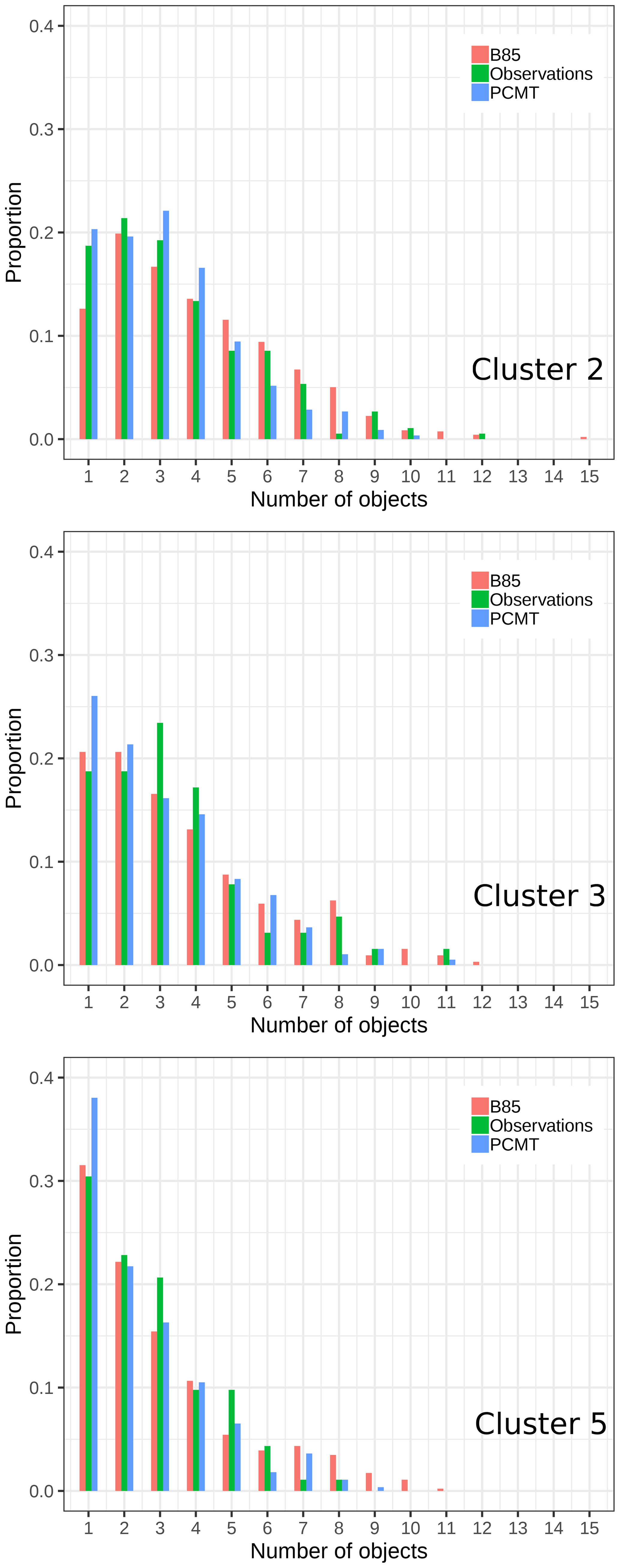
Figure 11 Normalized histograms of the daily number of SAL patterns, for the B85 physics scheme (red), PCMT (blue), and observation (green). Panels correspond to the three-cluster classification.

Figure 12 Distribution of the SAL first-pattern O₁ rain amount according to the number of patterns per day. Curves stand for the median of the distribution, and shaded areas range between the 25th and 75th percentiles. The dashed lines correspond to the second ranked SAL pattern O₂ rain amount.

More details about the magnitude of the objects can be produced by computing the integrated mass per object, M_k (see Sect. 2.3.1). First, for each day, objects are sorted from the largest to the smallest integrated mass. Integrated mass distribution of the two heaviest objects (noted O₁ and O₂) is then dispatched as a function of the number of objects for each cluster in Fig. 12. First, the range value of M is highly variable from one cluster to another. Maximum values are observed for cluster 3, while the magnitude for clusters 2 and 5 is comparable. The decrease in the mass for O₁ is clearer for cluster 3, meaning that a high number of objects over the domain leads to a natural decrease in the M value of the heaviest ones. We think that a part of the total integrated mass is then redistributed to the other objects. This is confirmed by O₂ curves since its mass increases with the number of objects. Conversely, for cluster 5, O₁ mass increases with the number of the objects, while O₂ is almost stable. The gap between O₁ and O₂ masses is at a maximum in the most extreme clusters (3 and 5). This suggests that when computing the volume V (see Eq. 7) and L2 (see Eq. 4), the weighted average is dominated by the object O₁. This implies that the verification could be considered a single-to-single object metric.

We now examine the ratio between the daily maximum rainfall of objects O₁ and O₂. This ratio ranges between 1.5 and 3, which means that O₁ represents the essential contribution of the daily rainfall peak. Since O₁ base area tends to be significantly larger that O₂, the information related to the inner object maximum rainfall is diluted in the large base area, resulting in a flat weak mean intensity of the object. This last result appears to support the fact that the SAL metric gives more weight to the object that contains the most intense rainfall.

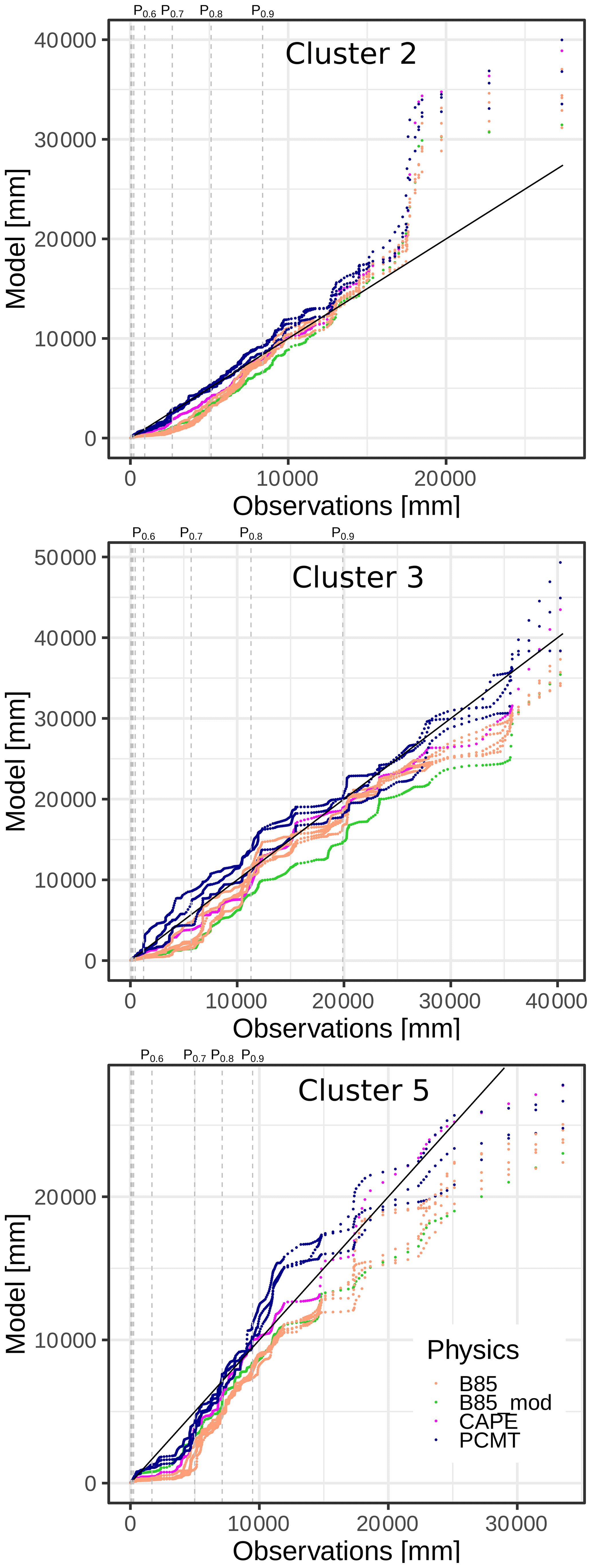
Figure 13 Quantile–quantile plot between SAL pattern rain amounts from the model (Y axis) and from the observation (X axis). Physics schemes are gathered into four classes (B85, PCMT, B85_mod, CAPE). Observation deciles correspond to the vertical dashed lines.

The comparison between the model reforecast physics and the observations is addressed using the whole distribution of daily mass M from the objects O_i identified across the full reforecast dataset, where i ranges between 1 and the total number N of objects. We proceed separately for each physical package. For a given scheme and cluster, the quantile values corresponding to the selected dataset are sorted in ascending order and then plotted versus the quantiles calculated from observations (Fig. 13). Half of the quantile distributions are not visible as they correspond to very weak pattern masses. For cluster 2 and PCMT physics most of the distribution of object mass is close to the observations. However all other physics distributions are skewed to the right compared to the observations for values below 10 000 mm. This behaviour is also observed for cluster 5 and it involves PCMT physics as well, for values between percentile 0.5 and percentile 0.7. Overall, in the quantile–quantile plot for cluster 5, the PCMT outperforms B85. In cluster 3, discrepancies between PCMT, B85, and the observations are of opposite sign, with PCMT being slightly above the observations, while B85 shows a weak underestimation. The CAPE physics distribution is left skewed compared to the observations and to the other physics. These results highlight some interesting properties of the models in predicting the rainfall objects. Except for some deviation concerning a few extreme cases of cluster 2 and a small portion of distributions of cluster 5, object mass distribution of physics is similar to the distribution drawn from the observation, especially for cluster 3. This means that the forecast is able to reproduce the same proportion of rainfall amounts inside a feature as the observations, even concerning the extreme right tail of the distributions, which corresponds to the major events of the series.

4 Summary and conclusions

In this study we have characterized the systematic errors of 24 h rainfall amounts from a reforecast ensemble dataset, covering a 30-year fall period. A 24 h rainfall observation reference has been produced on a regular grid with a resolution identical to the model in order to run point-to-point verification. We applied an object-based quality measure in order to evaluate the performance of the forecasts of any kind of HPE. Then, we took advantage of a rainfall clustering to analyse the dependence of systematic errors on clusters.

The selection of the HPEs within the reference dataset was based on a peak-over-threshold approach. The spatial regional discrepancies between HPEs are highlighted on the basis of the k-means clustering of the 24 h rainfall. Finally, we analysed the rainfall object properties in the model and in the observation to underline the rainfall field object properties for which the model acts distinctly.

The peak-over-threshold criterion leads to the selection of 192 HPEs, confirming that the most impacted regions are the Cévennes area and part of the Alps. The composite analysis for the five clusters shows that each cluster is associated with a specific class and location of 24 h precipitation events. It was found that 86 % of the number of HPEs are included in clusters 2, 3, and 5. Cluster 2 and 3 HPEs predominantly impact the Cévennes and Alps areas, while cluster 5 HPEs are located over the Languedoc-Roussillon region. Moreover, clusters 3 and 5 include the most extreme HPEs. Only diagnostics for clusters 2, 3, and 5 are considered.

The SAL object-quality measure has been applied distinctly to the 10 physics schemes (one per member) of the reforecast dataset and compared to the rainfall reference. It shows that the model’s overall behaviour for HPE forecasting is characterized by negative A components and positive S components. As in grid-point rainfall verification, all the SAL components get worse as a function of lead time. The model HPE rainfall objects tend to be more extended and less peaked. Even though their corresponding domain-average amplitude is weaker, it does not mean that the event maximum intensity is always weaker. This result is important, showing modellers that, even for intense rainfall events when orography interaction and quasi-stationarity mesoscale systems play a great role, the model tends to reproduce rainfall patterns with greater extension, rather than both smaller extension and weaker-intensity patterns.

In order to show regional disparities in the model behaviour, the SAL diagnostics have been divided according to the clusters and it shows interesting results. First, the A component negative contribution for the whole sample is higher, showing that on average more underestimation than overestimation is observed for the amplitude SAL component. It is notably the case for the most extreme clusters (over Cévennes and over Languedoc-Roussillon). However, when considering both positive and negative contributions to the integrated A component, the most extreme cluster (cluster 3) leads to better scores. This could mean that the variability of the A component is positively reduced for the most intense events. This is quite surprising and could reinforce the role of orography in this error decrease. As for the S-component distribution, we showed it is slightly positively skewed for clusters 2 and 3, while for cluster 5 the distribution of the S component is more centred. Likewise for the A component the integrated balance of positive and negative S-component contributions leads to better results for clusters 3 and 5. It is even more remarkable for cluster 5, for which the S component reaches the best score. Though it is difficult at this point to determine whether this characterizes an actual contrast in the model behaviour or if it is due to the physical properties of the cluster 5 events. One hypothesis could be related to the large number of single objects characterizing this cluster.

The impact of the different physics schemes has also been investigated, and it mostly emphasized the role of the deep-convection physical parameterization. Considering the SAL diagnostics, the two main deep-convection schemes, B85 and PCMT, clearly determine the behaviour of the model in HPE forecasting until lead time ranges longer than 3 d, after which no significant differences appear. This difference is clearly in favour of the PCMT scheme, which performs better than B85 for both SAL A and S components and in the majority of the subsampled scores considering the HPEs or the regional clusters. However, this PCMT asset is not huge, and both physics schemes can contribute to good or bad forecasts. The main significant difference is for the S component for the most intense rainfall, which shows that PCMT better approximates the structure of the rainfall patterns in these cases.

In light of the ability of our method to produce significant results even after several subsampling steps, we decided to study further statistical characterization of the SAL rainfall objects. It has been shown that in most cases, one large object stands out among other smaller objects, which often gathers the biggest part of the rain signal. For cluster 5, characterized by the Languedoc-Roussillon HPEs, the rainfall distribution could even be considered a single-object rainfall field. Then we focused on the ranked distributions (quantile–quantile analysis) of the object masses to compare the overall rainfall climatology of the model with the reference. First, this analysis showed that in particular the weakest precipitation is overestimated by all physics schemes. However, looking at the object mass distributions for the whole period, we find they are relatively close between all the physics schemes and the observation for most extreme rainfall events, especially for the PCMT deep-convection scheme. This statistical result implies that a global model should be able to reproduce a reliable distribution of rainfall objects along a long time period, e.g. the climate of the model and of the observations are close to each other. Therefore, in the case of PEARP, most of the forecast errors are mainly related to a low consistency between observed and forecasted fields, rather than to an inability of the prediction system to produce intense precipitation amounts.

This last result, objectively quantified for high-rainfall event thresholds (around 100 to 500 mm) on a long enough period, is important for two reasons. The first one concerns atmospheric modellers, showing that the physics schemes are able to reproduce climatological distributions of the most challenging rainfall events. On this basis, future research could investigate other sources of uncertainties like from the analysis set-up and implement ensuing model improvements. The model physics perturbation technique should then play a greater role in the control of the ensemble dispersion. From this perspective, the novel reanalysis ERA5 would be interesting to use, in particular its perturbed members, to improve the uncertainty from initial conditions in the reforecast. The second lesson to be learned from this study is that it is worth focusing on the study of model behaviour on intense event forecasting as it provides important learning to ensemble model end-users, in particular in the context of decision-making based on weather forecast. Quantifying systematic errors could also be used to favourably improve their inclusion in nested forecast tool processes.

In terms of methodology, this study also highlights that the combination of SAL verification and clustering is a relevant approach to show systematic errors associated with regional features for intense precipitation forecasting. This achievement is only enabled by the availability of a long reforecast dataset. This methodology could be further extended to a different model and another geographic region, on the condition of sampling a large number of HPEs.

The inter-comparison between some model physics deep-convection schemes and their role in HPEs predictability shows it is of course very sensitive for designing multi-physics ensemble forecasting systems. While the sensitivity to the initial perturbations was not studied in this work, the forecast of intense rainfall seems to be mainly driven by the classes of deep-convection parameterizations. Since the physical parametrization set-up is built by replicated schemes, the model error representation might lack an exhaustive sampling of the forecasted trajectories. Using more than two deep-convection parametrization schemes may improve the representation of model errors, at least for heavy-precipitation events.