Extreme wave analysis based on atmospheric pattern classification: an application along the Italian coast

This paper provides a methodology for classifying samples of significant wave-height peaks in homogeneous subsets in terms of the atmospheric circulation patterns behind the observed extreme wave conditions. Then, a methodology is given for the computation of the overall extreme value distribution by starting from the distributions fitted to each single subset. To this end, the k-means clustering technique is used to classify the shape of the wind fields that occurred simultaneously to and prior to the occurrences of the extreme wave events. This results in a small number of characteristic circulation patterns related to as many subsets of extreme wave values. After fitting an extreme value distribution to each subset, bootstrapping is used to reconstruct the omni-circulation pattern's extreme value distribution.

The methodology is applied to several locations along the Italian buoy network, and it is concluded from the obtained results that it yields a two-fold advantage: first, it is capable of identifying clearly differentiated subsets driven by homogeneous circulation patterns; second, it allows one to estimate high-return-period quantiles consistent with those resulting from the usual extreme value analysis. In particular, the circulation patterns highlighted are analyzed in the context of the Mediterranean Sea's atmospheric climatology and are shown to be due to well-known cyclonic systems typically crossing the Mediterranean basin.

1 Introduction

The extreme value theory is widely used for the analysis of extreme data in most of the geophysical applications. It allows us to estimate extreme (unobserved) values, starting from available records or modeled data, which are assumed to be independent and identically distributed (Coles, 2001). It is therefore crucial to identify homogeneous data sets complying with the abovementioned requirements before performing the extreme value analysis (EVA) of a given physical quantity.

When dealing with directional variables, it is common to group the data according to different directional sectors (Cook and Miller, 1999; Forristall, 2004), with such an approach being recommended in many regulations as well (API, 2002; ISO, 2005; DNV, 2010, among others). However, the use of directional sectors involves certain drawbacks. First, it cannot be employed for variables not being characterized by incoming directions (such as storm surge or rainfall). Second, data showing the same direction may be due to different forcing; in the context of wave climate, an example is of waves propagating in shallow waters being affected by refraction and/or diffraction. Finally, the borders of the directional sectors are often subjectively defined, without verifying if the data belonging to each subset are homogeneous and independent with respect to those of the other sectors (see Folgueras et al., 2019, in which they tackled this issue and proposed a methodology to overcome it).

An alternative approach to classifying the extreme events implies resorting to the atmospheric circulation conditions they are driven by and associating each extreme event with a particular weather pattern (referred to as WP). Such an approach has already been deep-seated in atmospheric sciences for the analysis of precipitations, snowfalls, temperature, air quality, and winds (Yarnal et al., 2001; Huth et al., 2008, among others). Nevertheless, there are few studies linking weather circulation patterns with the most likely induced sea states (e.g., wave climate and storm surge). Holt (1999) classified WPs leading to extreme storm surges in the Irish Sea and the North Sea. Guanche et al. (2013) simulated a multivariate, hourly sea-state time series in a location on the northwestern Spanish coast, starting with the simulation of a weather pattern time series. Dangendorf et al. (2013) linked the atmospheric pressure fields with the sea level in the German Bight (southeastern North Sea). Pringle et al. (2014, 2015) investigated how extreme wave events may be tied to synoptic-scale circulation patterns on the eastern coast of South Africa. Camus et al. (2014) proposed a statistical downscaling of sea states based on weather types, which is then applied to a couple of locations on the Atlantic coast of Europe to hindcast the wave climate during the twentieth century; it was also modeled under different climate-change scenarios. The latter methodology was improved by Camus et al. (2016), and further used by Rueda et al. (2016), for analyzing significant wave-height maxima. Solari and Alonso (2017) used a WP classification to perform an EVA of significant wave heights in the southeast coast of South America.

Except for Rueda et al. (2016) and Solari and Alonso (2017), none of the previous works focused on exploiting WP classification methodologies for defining the homogeneous data sets to be further employed for EVA. However, the two methodologies differ in several aspects. Rueda et al. (2016) dealt with the daily maxima of significant wave heights along with surface pressure fields and pressure gradients, averaged over different time periods, and applied a regression-guided classification to define 100 WPs. They subsequently fitted a generalized extreme value (GEV) distribution that estimated an extremal index from the daily maxima significant wave height of each WP, and from which they rebuilt the overall distribution of annual maxima (referred to as AM H_s). Despite the proposed methodology being able to reproduce the AM H_s distribution, it may be difficult to detect the most relevant physical processes behind the occurrence of extreme wave conditions with such a large number of WPs. Furthermore, as shown in Rueda et al. (2016), even though a large number of WPs was considered, only a few happened to significantly affect the EVA as most of the WPs that resulted were associated with mild wave conditions. Finally, retaining the daily maxima does not ensure that the data is independent, thus implying the need to use the extremal index. Instead, Solari and Alonso (2017) introduced a “bottom-up” scheme as follows: they first selected a series of independent extreme sea states; then, they identified a reduced number of WPs that allows us to group the selected data into homogeneous populations. A small number of WPs makes it easier to link the different subsets of extremes with known climate forcing. Above all, working with independent peaks allows us to rely on the classic and well-known extreme value theory, with no need to refer to additional indexes and/or more complex models that may be unfamiliar to many analysts.

In this paper, the methodology of Solari and Alonso (2017) is revisited and applied to several wave data sets along the Italian coastline. The objective of this research is twofold: (i) to explore how the definition of homogeneous subsets, based on WPs, affects the estimation of H_s extreme values; and (ii) to characterize the identified WPs in the framework of the Mediterranean region (MR) cyclone climatology.

The paper is structured as follows: in Sect. 2 we introduce the data and describe the methodology developed; the results are presented and discussed in Sect. 3; finally, in Sect. 4 conclusions are summarized and further developments are introduced.

2 Data and methods

2.1 Wave and atmospheric data

This paper takes advantage of eight hindcast points located in the Italian seas, as shown in Fig. 1. This choice allowed us to test the reliability of the proposed methodology under different local wave climates. In fact, the selected points are differently located along the Italian coastline, and, being exposed to different fetches, they are characterized by peculiar wave conditions. The same locations were taken into account by Sartini et al. (2015) when they performed an overall assessment of the different frequency of occurrence of the extreme waves affecting the Italian coasts. Table 1 reports the names, depths, and coordinates of the selected locations.

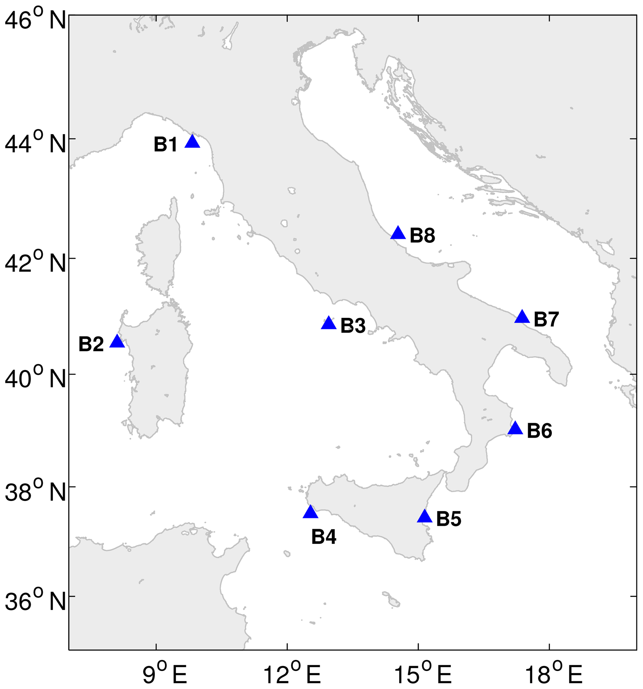
Figure 1 Study area and investigated locations with their respective codes.

Table 1 Long/lat coordinates and depths of the hindcast locations employed in the study (reference system: WGS84).

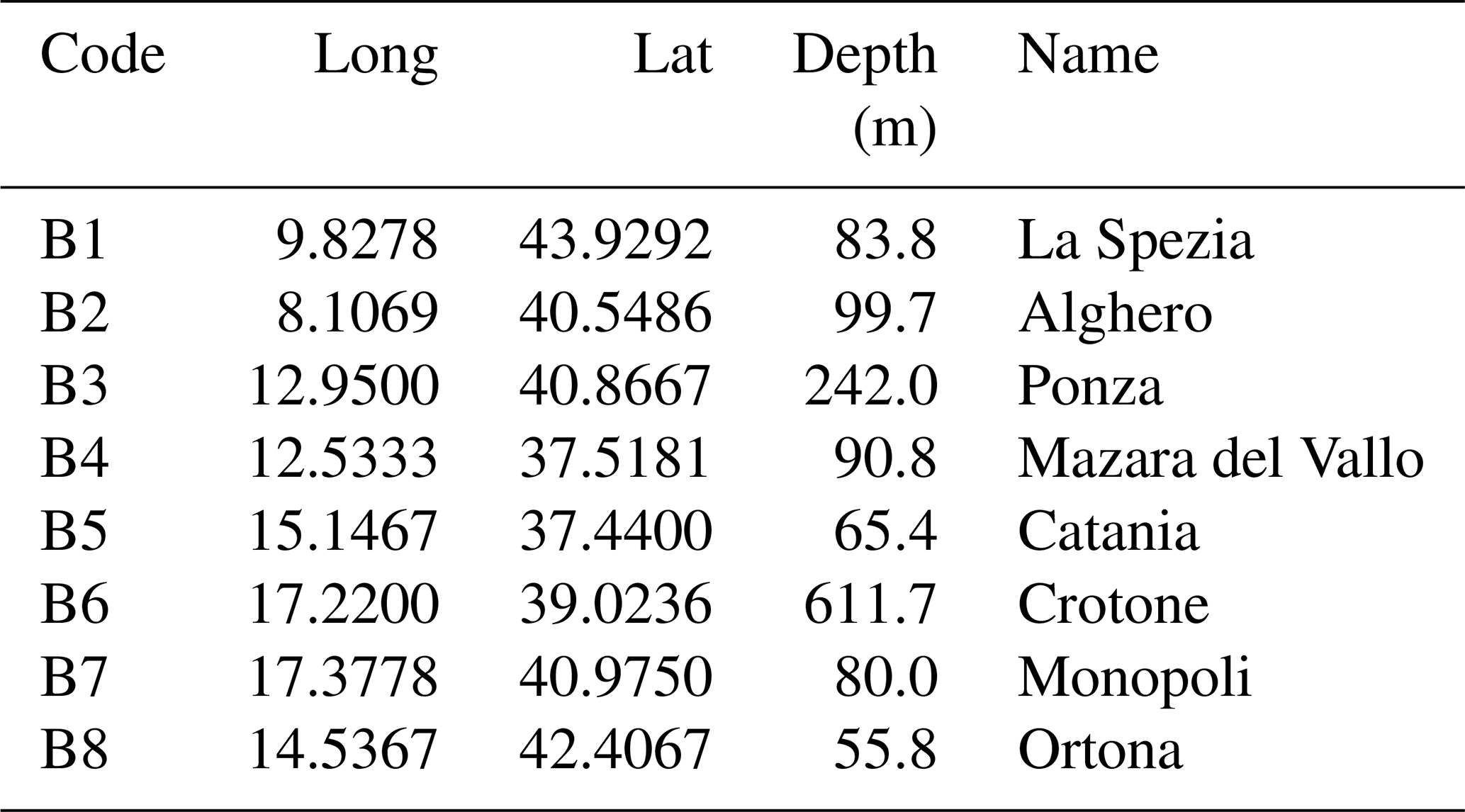
The points correspond to as many buoys belonging to the Italian Data Buoy Network (Rete Ondametrica Nazionale or RON; Bencivenga et al., 2012) that collected directional wave parameters over different periods between 1989 and 2012. Unfortunately, most of the buoys are characterized by a significant lack of data due to the malfunctions and maintenance of the devices. We therefore referred to hindcast data, since such a widespread lack of data would imply a loss of reliability for the following analysis. We relied on the hindcast of the Department of Civil, Chemical and Environmental Engineering of the University of Genoa (http://www3.dicca.unige.it/meteocean/hindcast.html, last access: 8 May 2020; Mentaschi et al., 2013, 2015). It now provides wave parameters on an hourly basis from 1979 to 2018 over the whole Mediterranean Sea, with a spatial resolution of 0.1^∘ in both longitude and latitude (however, at the time that the study was developed the series was defined up to 2016). Data were validated against the records of the buoys (when available); more details can be found in Mentaschi et al. (2013, 2015). The wind data used to drive the wave generation model were derived from the National Centers for Environmental Prediction (NCEP) Climate Forecast System Reanalysis (CFSR) for the period from January 1979 to December 2010 and the Coupled Forecast System model version 2 (CFSv2) for the period from January 2011 to December 2018, downscaled over the MR at the same resolution of the hindcast, along with the pressure fields, through the model Weather Research and Forecast (WRF-ARW version 3.3.1; see Skamarock, 2009; Cassola et al., 2015, 2016). These wind velocities data were used here to feed the cluster analysis of the wave peaks. It should be pointed out that, in the case of sea waves, other variables may concur to affect their propagation (and therefore the bulk parameters), i.e., the local bathymetry and the currents. However, the bottom depth is reasonably expected to not be relevant since all the locations investigated lie in deep water (see Table 1), and the currents were not fed into the wave model, but the hindcast data were widely validated and proved to be reliable.

2.2 Extreme event selection

For each location, wave-height peaks were selected through a peak-over-threshold (POT) approach, and in particular by using a time-moving window. This approach works as follows. First, the whole series of H_s is spanned through a time-moving window of given width; second, when the maximum of the data within the window happens to fall in the middle of the window itself, it is retained as a peak; finally, in order to get rid of the peaks which are not related to severe sea states, a first H_s threshold is chosen and only peaks exceeding this threshold are retained for further analysis.

In this study, the width of the moving window was set equal to 1 d, meaning that the inter-arrival time between two successive storms is at least equal to 1 d for each location. The threshold was fixed as the 95th percentile of the resultant peaks. This ensured that a uniform approach for all the locations was maintained by efficiently capturing the different features of the local wave climates. Besides the significant wave heights, we also retained the waves' mean incoming directions corresponding to the peaks (θ_m), which were used for analyzing the outcomes of the clustering algorithm. Finally, we extracted the mean sea level pressure field (MSLP) and surface wind fields for several time lags (0, 6, 12, 24, 36, and 48 h earlier with respect to the peak's date) for each peak over the whole MR. Wind fields were used to classify the selected peaks due to their parent WP, as described in the following section; MSLP fields were used instead for the postprocessing and climatological analysis of the results.

2.3 Extreme event classification: definition of weather patterns

The classification of extreme events is based on surface wind fields (${\stackrel{\mathrm{‾}}{u}}_{\mathrm{w}}$) observed in the whole MR during the hours before and concomitant to the time of the peaks. In order to define the spatial and temporal domains to be taken into account, we looked at the correlation maps between the wind velocities and the H_s peaks for different time lags. Correlations were evaluated over a subgrid of the atmospheric hindcast, with nodes spaced of 0.5^∘ in both longitude and latitude. Computing the correlation between the H_s and ${\stackrel{\mathrm{‾}}{u}}_{\mathrm{w}}$ series is not straightforward, as the former variable is scalar and the latter is directional. To tackle this issue, we followed the procedure suggested by Solari and Alonso (2017). Given a time lag Δt, the wind is defined by its zonal and meridional components $(u_x,u_y{)}_{(i,j,\mathrm{\Delta }t)}$ at every node (i,j); thus, the correlation between H_s peak series and the time-lagged surface wind speed at any given node is estimated as the maximum of the linear correlations obtained by projecting the wind speed series in all the possible directions. This is calculated as follows:

$$\begin{array}{}\text{(1)}& {\mathit{\rho }}_{(i,j,\mathrm{\Delta }t)}=\underset{\mathrm{0}\le \mathit{\theta }<\mathrm{2}\mathit{\pi }}{max}\left\{\mathit{\rho }\left(H_{\mathrm{s}};{\stackrel{\mathrm{‾}}{u}}_{\left(i,j,\mathrm{\Delta }t,\mathit{\theta }\right)}\right)\right\},\end{array}$$

where ${\mathit{\rho }}_{i,j,\mathrm{\Delta }t}$ is the resulting correlation for node (i,j) at time lag Δt, ρ refers to linear correlation function, and $u_{\left(i,j,\mathrm{\Delta }t,\mathit{\theta }\right)}$ is the surface wind speed projected along direction θ according to Eq. (2):

$$\begin{array}{}\text{(2)}& {\stackrel{\mathrm{‾}}{u}}_{\left(i,j,\mathrm{\Delta }t,\mathit{\theta }\right)}=u_{x(i,j,\mathrm{\Delta }t)}\cos \left(\mathit{\theta }\right)+u_{y(i,j,\mathrm{\Delta }t)}\sin \left(\mathit{\theta }\right).\end{array}$$

In this way, not only is a maximal correlation obtained for every node but also the direction corresponding to the maximal correlation, which is estimated as follows:

$$\begin{array}{}\text{(3)}& {\widehat{\mathit{\theta }}}_{\mathit{\rho }(i,j,\mathrm{\Delta }t)}=\underset{\mathrm{0}\le \mathit{\theta }<\mathrm{2}\mathit{\pi }}{\mathrm{argmax}}\left\{\mathit{\rho }\left(H_{\mathrm{s}};{\stackrel{\mathrm{‾}}{u}}_{\left(i,j,\mathrm{\Delta }t,\mathit{\theta }\right)}\right)\right\}.\end{array}$$

The correlation maps computed with Eq. (1) allowed us to evaluate the spatial domain and the time lags for which ${\stackrel{\mathrm{‾}}{u}}_{\mathrm{w}}$ is significantly correlated (i.e., directly affecting) to the resulting wave peaks at a given location.

Once the spatial and time domain of the wind fields producing the peak wave conditions were defined, the wind fields were used for clustering and classifying the extreme events. To this end, the k-means algorithm was used and fed with the normalized wind fields. The k-means algorithm is aimed at partitioning an N-dimensional population into k sets (clusters) on the basis of a sample, in order to minimize the intracluster variance (MacQueen, 1967). The normalization of the wind fields sought to reduce the influence of the intensity of the wind speed on the classification, so that only the spatial form of the field and its time evolution were taken into account. Note that the values of H_s did not play any role in the classification of the peaks but rather the identification of the point in time of the wind fields.

2.4 Analysis of the WP climatology

Once the wind fields, and therefore peak H_s series, were grouped into k clusters, the MSLP corresponding to the events within each cluster were averaged, and the position of the lowest pressure was recorded for all the Δt taken into account. This allowed us to track the paths of the averaged low-pressure systems corresponding to each cluster and in turn define the respective WP.

At a second time, the dynamics of the systems were compared with those of the cyclones typically detected in the Mediterranean Sea (Trigo et al., 1999; Lionello et al., 2016), while the frequency of occurrence of the events of different clusters was compared with the outcomes of Sartini et al. (2015). The number of clusters needed to group the series was defined for every location by looking at the outcome of the cluster analysis: when an increase from k to k+1 clusters did not further lead to a new, clearly differentiated WP, the research was stopped and k was used for the cluster analysis of that particular location.

2.5 Extreme value analysis

The EVA was performed independently over the subsets of H_s peaks resulting from the cluster classification. We followed the methodology proposed by Solari et al. (2017), where the threshold for the POT analysis is estimated as the one maximizing the p_value of the upper tail Anderson–Darling test. Then, once the threshold is identified (i.e., a subset of the peaks within a given WP is defined), the three parameters of the generalized Pareto distribution (GPD) are estimated through the L-moments method, and the return-period (T_r) quantiles of the variable under investigation are computed. In this paper, in order to estimate the overall T_r–H_s curve and its confidence intervals from the GPDs fitted to each WP, a bootstrapping approach was implemented (Table 2). The algorithm in Table 2 shows a pseudocode summarizing the bootstrapping procedure. First, N_boot series of H_s, each N_years long, are generated for every WP. Second, the series generated for the different WPs (N_WP per location) are combined in order to obtain one single N_years long series for each of the N_boot simulations. Third, an empirical relationship between T_r and H_s (i.e., an empirical cumulative distribution function or ECDF) is estimated from each one of the N_boot series. Lastly, the expected value and confidence intervals of H_s are estimated from the N_boot ECDFs for several return periods.

Table 2 Computational scheme of empirical extreme values curves and its confidence intervals.

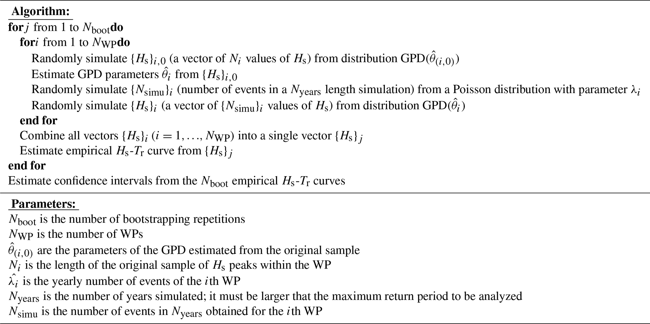
The method assumes a Poisson–GPD model for each WP and that the realizations of different WP are independent of each other. This independence hypothesis was evaluated by estimating the correlation between the annual number of peaks associated with each WP.

For a given location, the overall workflow can be summarized as follows:

• selection of a series of H_s peaks through a POT approach;

• selection of the wind field data to be employed in the clustering algorithm (i.e., Δt and spatial domain);

• classification of the H_s peaks due to the k-means algorithm;

• definition of a suitable number (k) of WPs;

• averaging of the MSLP corresponding to the peaks of each WP, for each Δt taken into account;

• performing EVA over the single subsets; and

• computation of the overall long-term distribution through a bootstrapping technique.

This methodology was applied to all the hindcast locations shown in Fig. 1. In this paper, for the sake of clarity, just the results of the locations B4 (Mazara del Vallo) and B7 (Monopoli) are shown and discussed. Indeed, just one WP was necessary for classifying the peaks in La Spezia and Alghero (B1 and B2); thus, no further analysis was performed. Among the locations left, we simply selected the locations furthest from each other in the east–west direction. However, the results relating to the other locations can be found in the Supplement.

3 Results and discussion

Once the series of H_s peaks is selected, the first step of the proposed methodology requires us to define the domains of ${\stackrel{\mathrm{‾}}{u}}_{\mathrm{w}}$ in time and space due to the outcomes of the correlation analysis between the two parameters. Indeed, as mentioned in Sect. 2.1, the wind is reasonably expected to play a major role in the observed wave parameters at the investigated locations. Figure 2 shows the correlation maps for B7 for different time lags, along with the directions leading to the maximum values of correlation in each node. It is interesting to see how $\widehat{\mathit{\theta }}$ for Δt=0 h are distributed along the nodes characterized by similar values of ρ. Actually, even though the values of $\widehat{\mathit{\theta }}$ come from a purely statistical analysis (i.e., they were computed with Eq. 3), their spatial distribution follows that of a typical cyclone. The velocities happen to be uniformly oriented along the nodes characterized by the higher values of ρ, which is close to tangential to a circle centered on the nodes showing lower values of ρ instead. This allows us to get insight into the predominant process most likely affecting the wave climates of the investigated locations, and it will be discussed later on in this paper. On the contrary, the analysis of the correlations between H_s and ${\stackrel{\mathrm{‾}}{u}}_{\mathrm{w}}$ reveals that the areas characterized by similar values of ρ are not uniformly distributed in the neighborhood of the points considered. It is therefore difficult to uniquely contour the nodes to be taken into account for the successive analysis. As regards the time step, correlations rapidly decrease for Δt longer than 12 h, after which no evidence of significant ρ can be observed. The same outcomes apply for all the other locations taken into account. Results suggest that the events shall be linked to broader circulation patterns. In view of the above, it was decided to refer to the whole MR and time lags of 0 and 12 h for the purposes of peak classification.

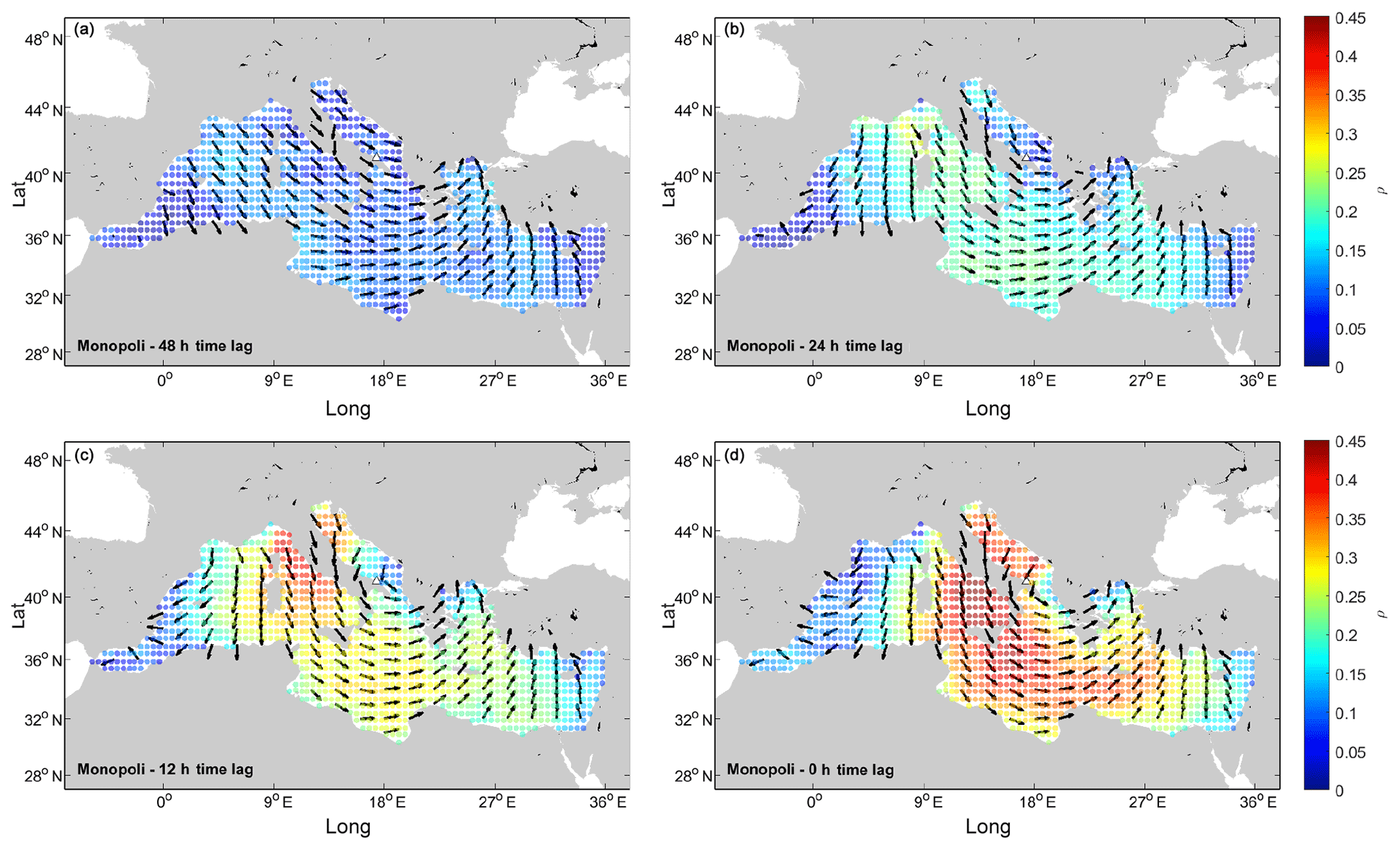
Figure 2 Correlations between H_s and ${\stackrel{\mathrm{‾}}{u}}_{\mathrm{w}}$ in location B4 for different time lags. (a) Δt equals 48 h; (b) Δt equals 24 h; (c) Δt equals 12 h; and (d) Δt equals 0 h.

Once the spatial and temporal limits of the wind fields to be used in the k means were defined, we performed a sensitivity analysis on the resultant average MSLP belonging to each cluster among the total number of tested clusters (k). Two clusters were needed to detect different systems at all the sites, except for Alghero and La Spezia where the local extreme waves could be related to a single pattern. For the other locations, increasing k did not lead to the systems significantly diverging from those already defined. The reason for such a small number of resulting WPs has to be found in the nature of the H_s employed in the analysis. Indeed, these are associated with extreme sea states, which are most likely driven by atmospheric phenomena developing along well-defined and fixed tracks.

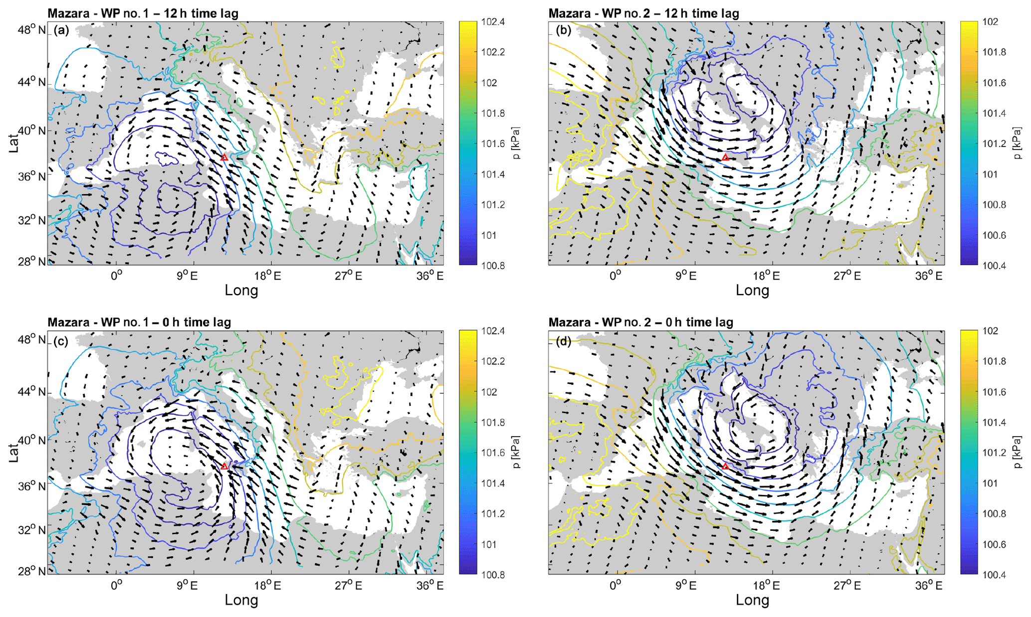
Figure 3 Average MSLP for the H_s peaks in Mazara del Vallo (B4). (a) WP#1, Δt equals 12 h; (b) WP#2, Δt equals 12 h; (c) WP#1, Δt equals 0 h; and (d) WP#2, Δt equals 0 h.

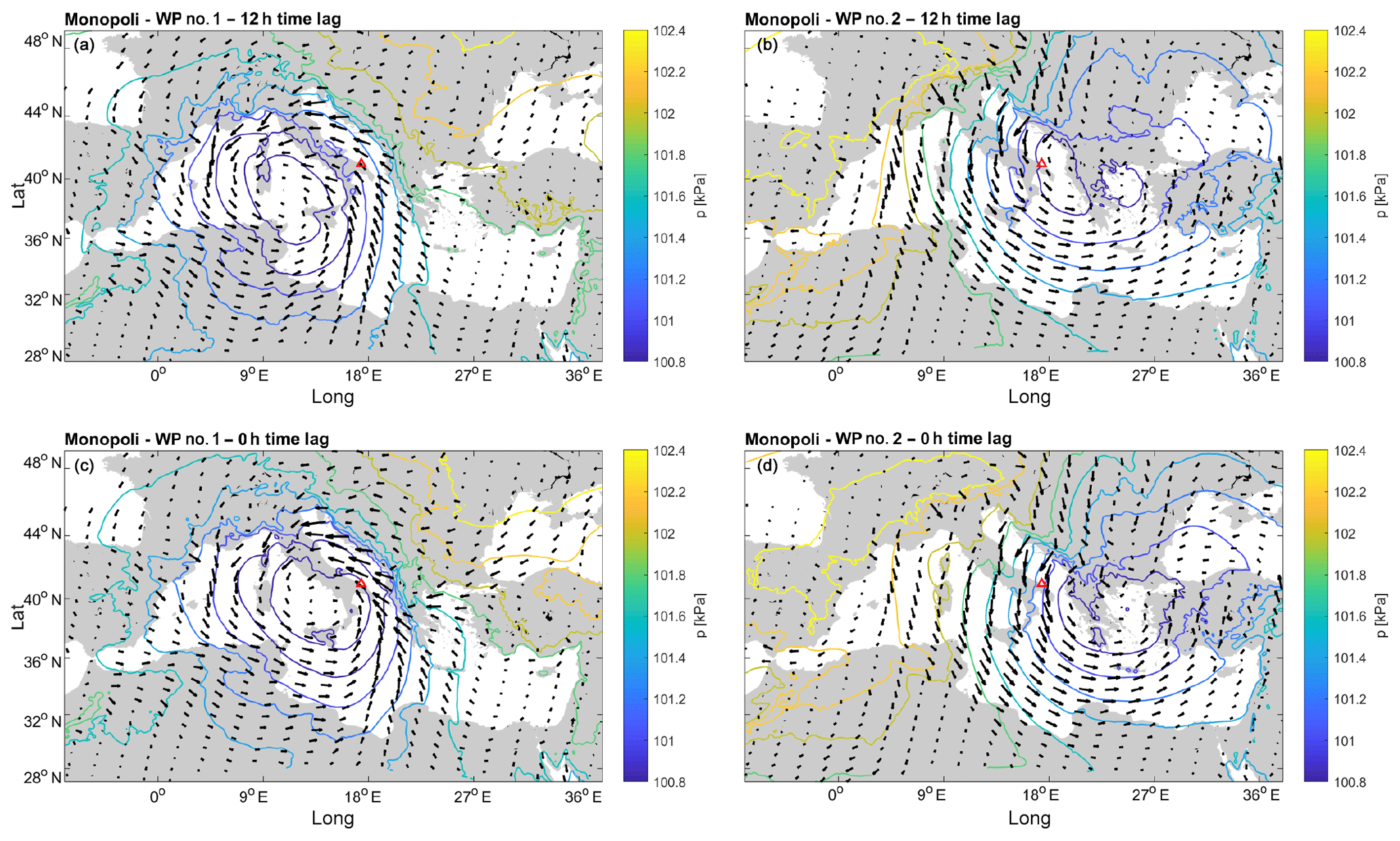
Figure 4 Average MSLP for the H_s peaks in Monopoli (B7). (a) WP#1, Δt equals 12 h; (b) WP#2, Δt equals 12 h; (c) WP#1, Δt equals 0 h; (d) WP#2, and Δt equals 0 h.

Figures 3 and 4 show the averaged pressure fields corresponding to both the clusters and Δt in the B4 and B7 hindcast points. Here, two main systems can be clearly distinguished, namely (i) a low-moving SW–NE towards the Balkan area (say WP#1) and (ii) a low-moving NW–SE (henceforth referred to as WP#2).

Let us first focus on WP#2. The low pressure moves SE from central Europe, crossing the Adriatic Sea, and decreasing its intensity once it gets to the south Balkan area where it stops until it finally dissolves. Regarding WP#1, the cyclogenesis most likely takes place in the eastern area of North Africa, with cyclones first approaching the western coastline of Italy while moving NE. The paths of WP#1 and WP#2 show interesting similarities with well-known cyclones typically forming and departing from two of the most active cyclogenetic regions in the MR, respectively, in the lee of the Atlas Mountains and the lee of the Alps (Trigo et al., 1999). The MSLP composites related to WP#1 and WP#2 are consistent with those highlighted in previous research, for instance Lionello et al. (2006), showing the synoptic patterns associated with extreme significant wave heights in different regions of the Mediterranean Sea (see in particular the MSLP fields reported in Fig. 122a and d of Lionello et al., 2006 for WP#2 and WP#1, respectively). In particular, WP#2 seems to follow the Genoa system path that usually moves down to the Albanian and Greek coasts, while that of WP#1 shows characteristics analogous to the Sharav depression by moving northeastward toward the Greek region (Flocas and Giles, 1991; Trigo et al., 1999, 2002).

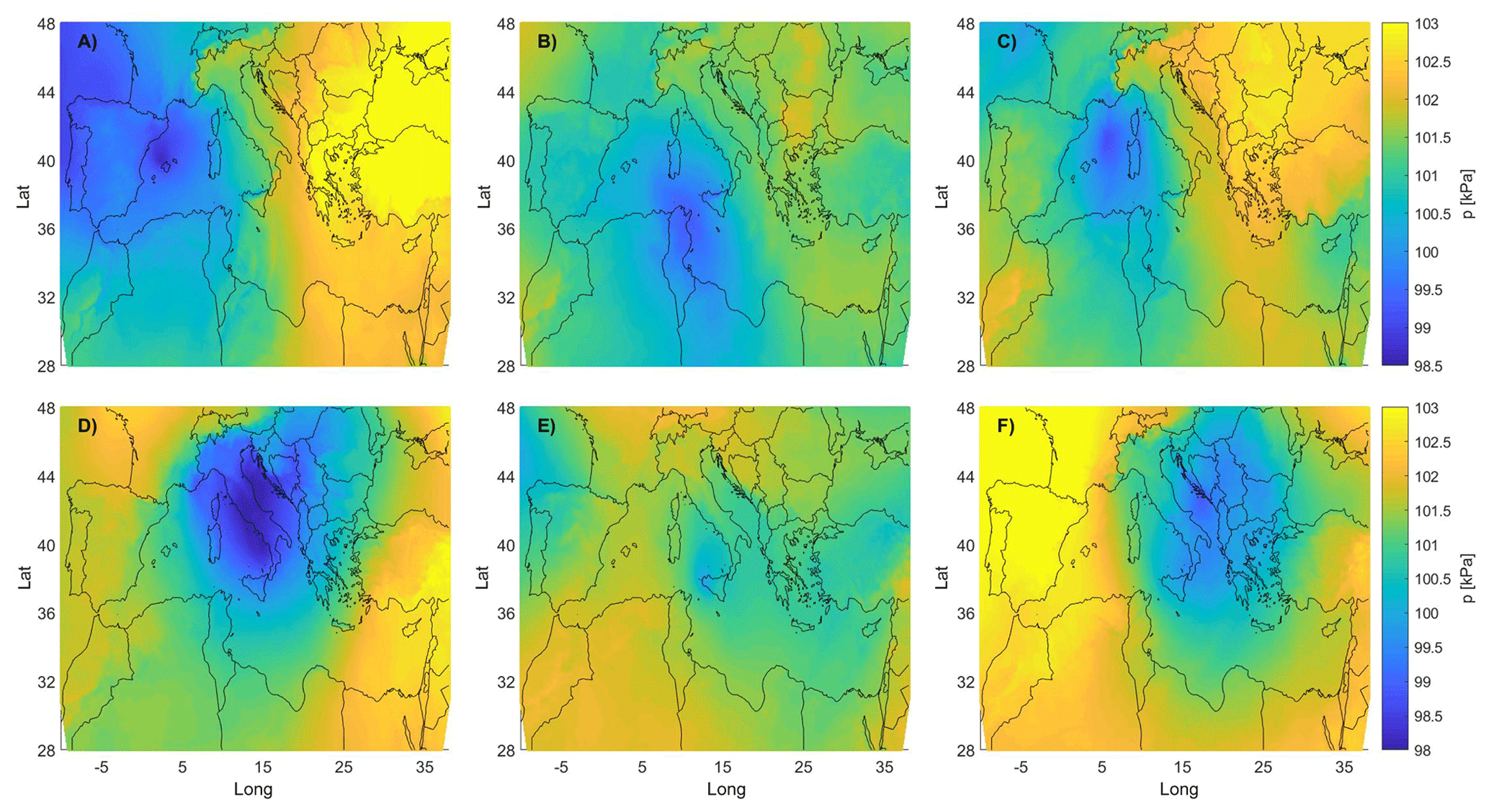
Figure 5 MSLP associated with the three highest POT events in Mazara del Vallo (B4). (a–c) WP#1 events; (d–f) WP#2 events. The storms are sorted from left to right in descending order.

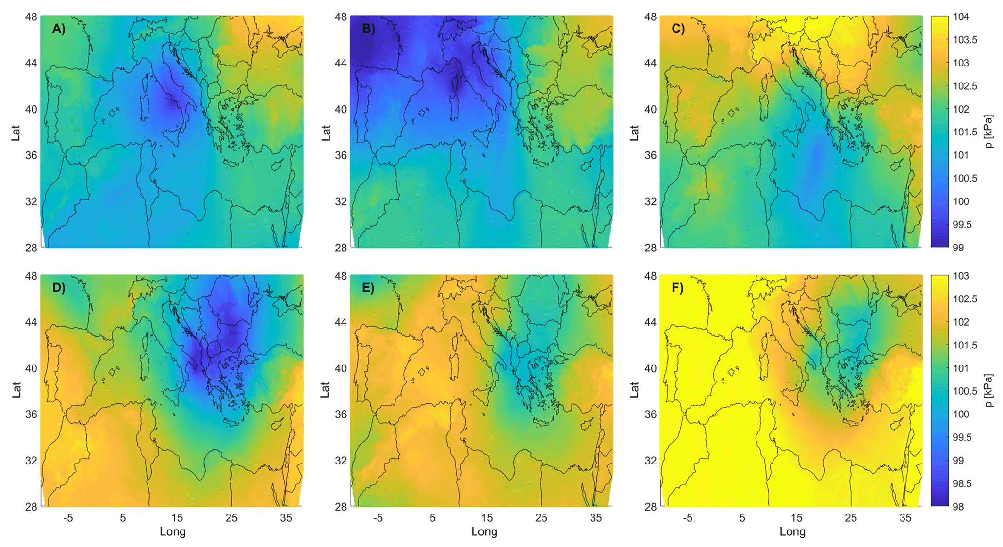
Figure 6 MSLP associated with the three highest POT events in Monopoli (B7). (a–c) WP#1 events; (d–f) WP#2 events. The storms are sorted from left to right in descending order.

At a second time, the MSLP related to the three highest events for both the locations and the WPs were individually analyzed in order to evaluate their homogeneity with respect to the overall MSLP averages. The results are shown in Figs. 5 and 6.

From the MSLP charts of Figs. 5 and 6, it can be seen how low pressures are in good agreement in terms of their locations and, in turn, with the average MSLP fields reported in Figs. 3 and 4. Actually, this especially applies in the case of the WP#2 events: the location of the low pressure of the cyclone is similar for the analyzed storms, though there are differences in terms of the absolute value of the pressure and slight differences in the shape of the cyclone too (the values of the color scale were modified to better appreciate the locations of the lows). This is something to be expected, as it partially explains the different intensities of H_s (of course, local effects have to be taken into account as well). However, there is an important degree of variability within each family of events, particularly regarding WP#1.

The paths highlighted for WP#1 and WP#2 characterize the lows of the WPs detected in all the investigated sites (see the Supplement). A summary of the low position at the two different Δt can be appreciated in Fig. 7, which reports the tracks of both the WP#2 and WP#1 systems in all the sites but B1 and B2; indeed, in the latter cases the analysis of the MSLP fields did not allow us to identify two separated systems.

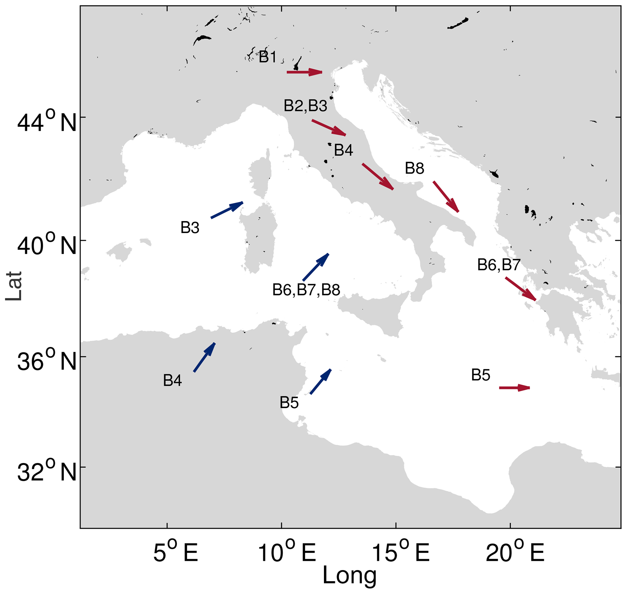
Figure 7 Time evolution of the center of the low pressure for the different WP identified for each buoy. In blue – WPs with lows traveling northeastward (WP#1); in red – WPs with lows traveling eastward or southeastward (WP#2).

It is interesting to see how the WP#2 low moves across the investigated sites in a precise, chronological order, first crossing the northernmost locations and then those next to the south Balkan area where the cyclone actually ends its run. As such, we took four buoys affected by WP#2 at different times as a reference by evaluating the time lag between the respective peaks generated by such a system. For each storm, we considered the extreme series of B4, computing the time lag between the peak at the buoy and peaks occurring in B2 and B1 (occurring earlier) and B6 (occurring later); the distributions of the time lags are shown in Fig. 8.

Figure 8 Relative frequency of the events' delay for B2, B1, and B6. Referring series is that of B4.

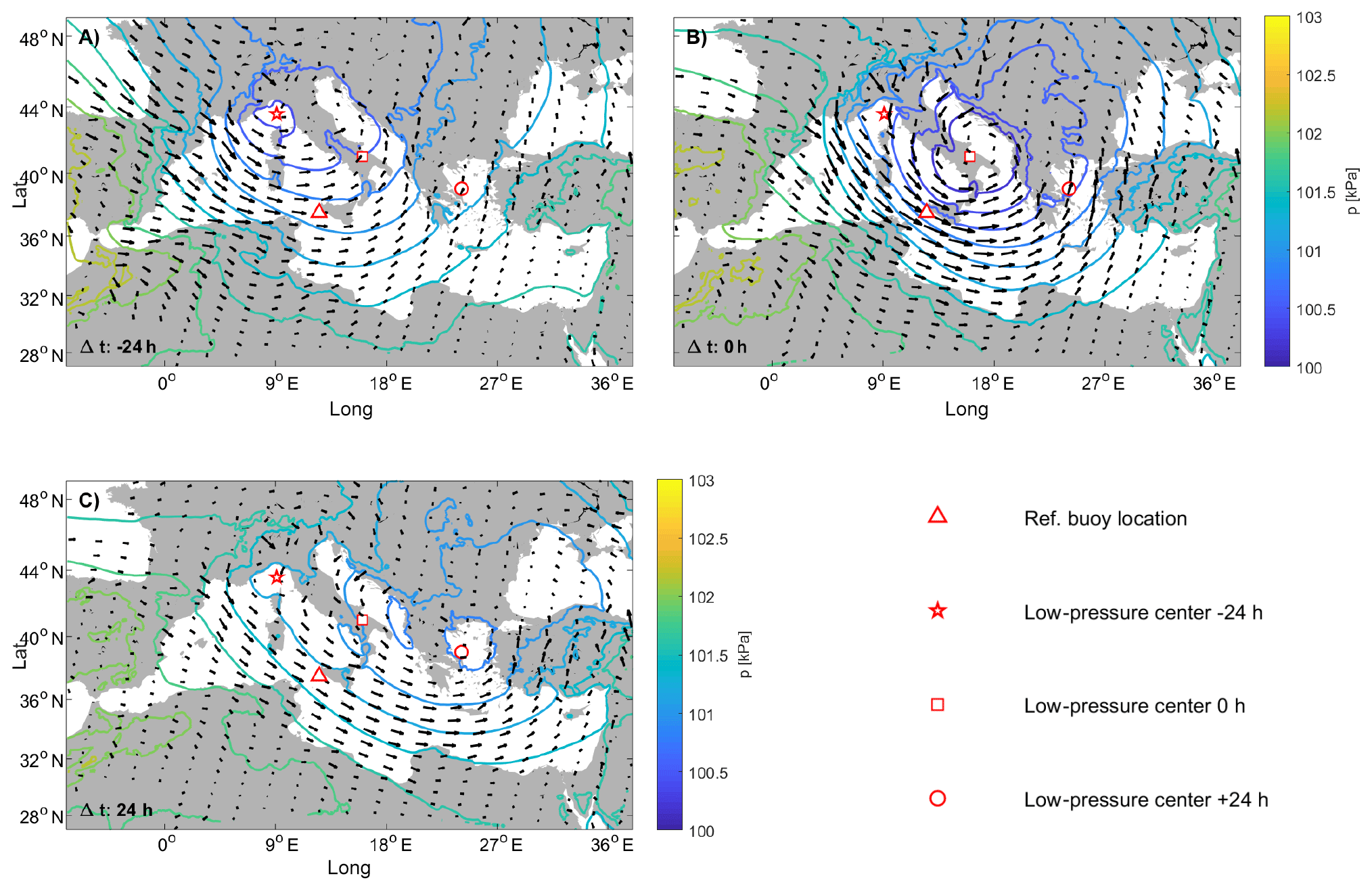
Figure 9 WP#2: average MSLP evolution with respect to the reference dates of the events in B4 (underlined with the red triangle).

Looking at Fig. 8, it is evident how the majority of the events' delays between B4 and the other investigated points fall within about 40 h. We therefore evaluated the average MSLP fields for time lags up to 48 h before and after the storms occurred at the reference location, tracking the low-pressure-center evolution. Results show how the cyclone runs out in a couple of days as the center of the low travels at approximately 1600 km, with a resulting speed of ∼33 km h⁻¹ (see Fig. 9). Both the lifetime of the identified cyclone and the speed at which it moves are compatible with the features of the cyclones most frequently encountered in the MR (Lionello et al., 2016). Unfortunately, regarding WP#1, an equally clear path cannot be detected since the average lows apparently arise simultaneously in most of the points taken into account. As previously pointed out, the MSLPs related to this pattern show a higher variability with respect to those characterizing the events of WP#2; thus, they would require further deepening and more detailed investigations. Therefore, we did not characterize the mean evolution of the MSLP fields related to the events of WP#1.

Figure 10 Monthly number of events for different WPs. (a) B4; (b) B7.

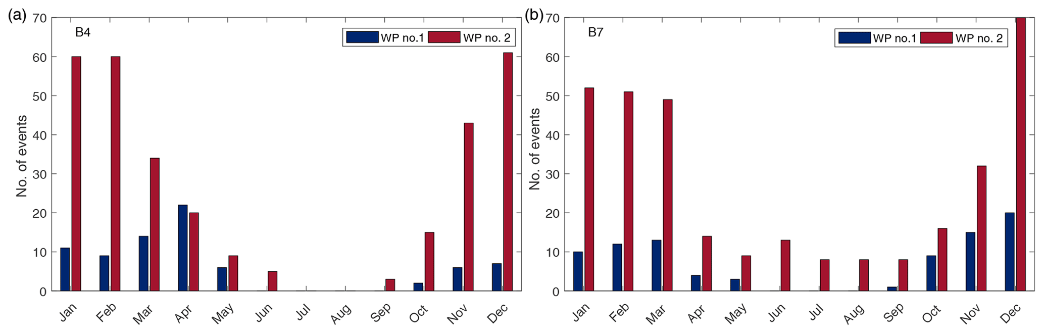
The characterization of the two systems is reflected in the frequency of the occurrence of the storms, with the peaks belonging to different subsets also showing distinctive seasonality. From the results shown in Fig. 10, it can be seen how WP#2 peaks mainly occur in winter, whereas the events of WP#1 are characterized by two milder intra-annual peaks of occurrence that are spread among the spring and autumn months. The intra-annual cycle of the WP#1 events further suggests a direct link with the Sharav cyclones, which show similar seasonal fluctuations; regarding the WP#2 peaks, even though the storms of the Genoa low are more uniformly distributed throughout the year, the most intense events occur precisely during winter as it happens in the abovementioned locations (details can be found in Lionello et al., 2016).

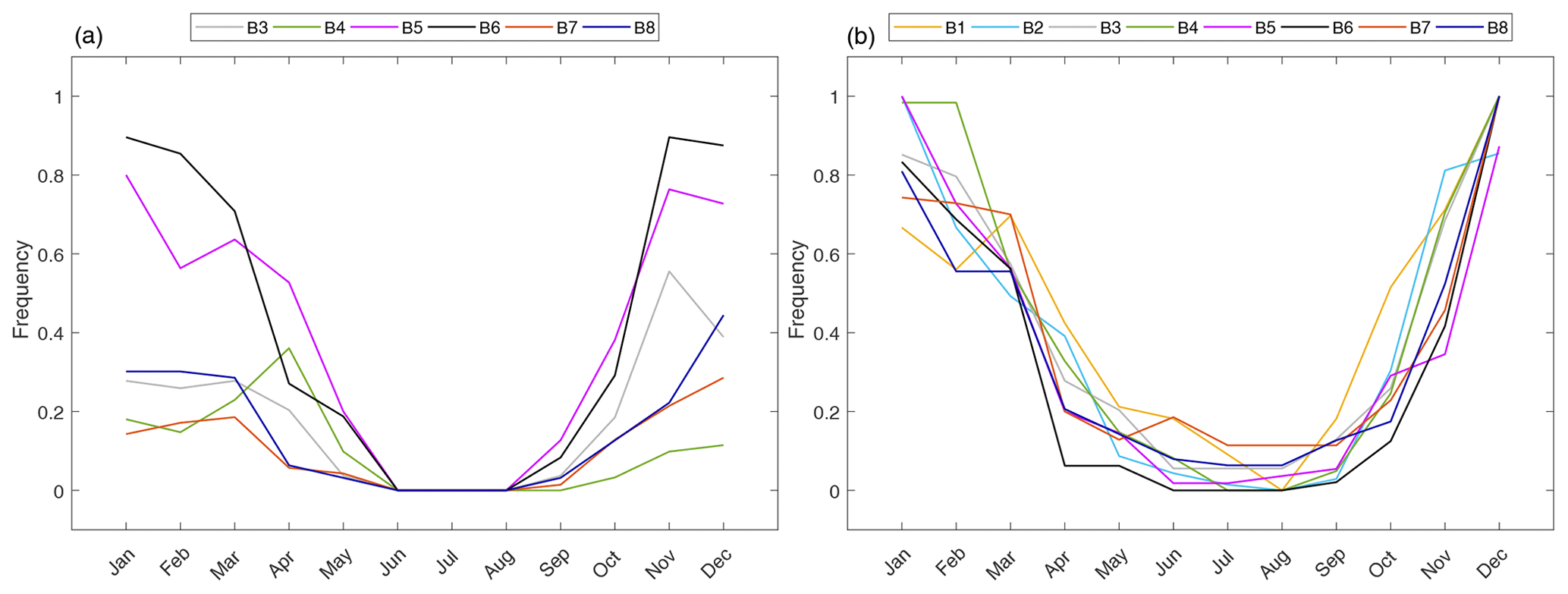
Figure 11 Normalized monthly frequency of occurrence of the extremes. (a) Events belonging to WP#1; (b) events belonging to WP#2.

Figure 11 summarizes the results of the monthly frequency of occurrence of the extremes in all the investigated locations, which are grouped according to the WP. For each location, frequencies were normalized in the 0–1 space with respect to the total number of peaks, in order to be able to compare the outcomes defined over different ranges.

It can be seen how the relative weight of WP#1 events on the overall peaks distributions increases when moving south. Points in the northernmost locations (B1 and B2) are apparently not influenced by the WP#1 system, and their extreme waves are actually linkable to just WP#2. Moving to the southernmost locations (B5 and B6), no significant differences in the seasonality of the two patterns' events can be appreciated; in these two buoys, none of the two systems shows a prevailing frequency of occurrence for the induced storms.

The aforementioned behavior may be justified by looking at the location of the investigated points (see Fig. 1) as follows: lows moving northeastward directly run over B5 and B6, marginally affect B7, B8, B4, and B3, whereas they do not interest B1 and B2. However, position of the buoys with respect to the cyclones' paths is not the only relevant variable. Indeed, local bathymetry and prevailing fetch characteristics may result in storms having, on average, unique characteristics; e.g., it may happen that peaks related to the same WP show distinct frequencies of occurrence, for instance the events related to WP#1 in B6 and B7. In this latter case, the predominant parameter seems to be the fetch length, which is very limited for B7 with regards to the NE incoming waves (precisely related to the first weather-circulation pattern).

The WPs that are defined in the present study show common characteristics with those qualitatively identified by Sartini et al. (2015) in a seasonal variability analysis of extreme sea waves. In particular, the same WP was identified in B1 and B2, linking the extremes with the Gulf of Genoa cyclogenesis WP type. As Sartini et al. (2015) noted, even if cyclones in the Gulf of Genoa are a constant feature over the whole year, those connected at the extreme events are the ones characterized by the lowest value in MSLP. These findings (i.e., higher values during the winter rather than in spring and summer time) were observed in the southern Tyrrhenian Sea as well (for instance in B4) and in the central Tyrrhenian Sea (B3). In the latter case, we found a more marked seasonal variation of the extremes, as the two resultant WPs are well separated between winter and autumn. Intra-annual variability was observed also for B7, while the analysis carried out by Sartini et al. (2015) did not reveal this kind of behavior; analogously, B5 and B8 buoys revealed the presence of two distinct WPs, while the previous analysis identified just one cyclogenesis system. These differences may be justified in the first place by the different peak selection (a moving window for this study, while Sartini et al., 2015, use a partial duration series approach). Moreover, evaluation of the seasonality follows completely different algorithms: the present study directly applies a clustering technique over the selected peaks, while the former analysis used the peaks to model a time-dependent distribution, further characterizing their seasonality on the basis of the values of the distribution coefficient generated by the fitting procedure.

Figure 12 Scatterplot of H_s and θ_m due to different WP. (a) B4; (b) B7.

Another interesting outcome regards the characteristics of the extremes differentiated due to the parent clusters following the k-means algorithm. Figure 12 shows the covariates H_s and θ_m of the selected peaks belonging to each WP.

Looking at the scatter plots, it can be appreciated how the events belonging to different clusters are remarkably homogeneous in terms of wave–bulk parameters, even though the latter were not used for clustering the peaks. In the case of B4, where it is clearly a bimodal distribution with respect to the waves' incident direction (i.e., two peaks corresponding to SE and NW), the proposed methodology allows us to differentiate the sea storms according to the directional frames of the local wave climate. On the other hand, when the waves' direction is more uniformly scattered over a given sector, it is not unusual that different climates force results in the same wave direction; this can be seen in B7, where θ_m-H_s scatters belonging to different patterns are partially overlapped. Thus, a directional classification is not straightforward and would most probably not be able to differentiate the storms due the cyclones generating them. Nevertheless, in such a case the distributions of H_s are also homogeneous within each WP, with the more severe H_s related to the WP#2 system in both the locations.

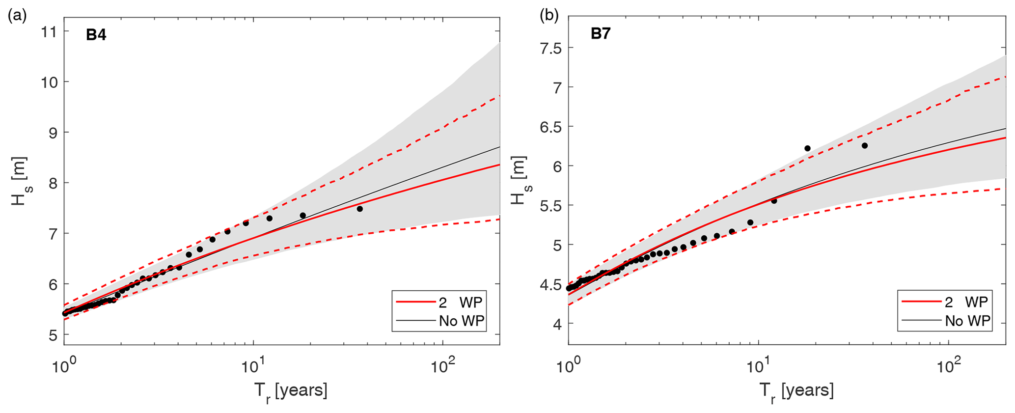
Figure 13 Omni-WP extreme value distributions of H_s obtained from the whole set of peaks (black) and from combining single-WP distributions (red), along with 90 % confidence intervals (gray shading and red dashed lines, respectively). (a) B4; (b) B7.

Finally, Fig. 13 shows the T_r-H_s curves, by comparing the results obtained directly from the whole set of peaks with those obtained from the single-WP distributions, and combines them by means of the algorithm given in Table 2 (i.e., omni-WP curves).

The omni-WP curves show a remarkable agreement with those carried out through the analysis of the whole data set without WP classification. In both the B4 and B7 locations, it can be even appreciated that there is a narrowing of the confidence intervals, which means a reduction in the total variance for the long-term estimates. Actually, the curve related to B4 shows a slight deviation between the two approaches (≃30 cm over the 200-year wave); however, such small magnitudes imply relative errors of ≃4 % with respect to the omni-WP curves and can be therefore considered as an uncertainty inherent in this kind of computations (see, e.g., Borgman and Resio, 1977, 1982, stating that reliable long-term estimates can be carried out just up to three times of the yearly length of the original data set).

These results seem to reinforce the validity of developing the omni-WP curve under the hypothesis of independence between the events of different WPs. In this case, the independence hypothesis was to some extent corroborated by the low correlations values attained by the intraclusters annual frequency of occurrence for all the locations as follows: −0.17, 0.23, −0.13, −0.11, −0.34, and 0.13 for B5, B6, B4, B7, B8, and B3, respectively. In conclusion, it is good to recall that thresholds for the EVA were selected in order for the peaks to come from a generalized Pareto family (Solari and Alonso, 2017), thus guaranteeing the intracluster homogeneity of the data.

4 Conclusions

In this paper, the extreme sea storms at eight hindcast points that are differently located along the Italian coasts were analyzed. The investigated locations are characterized by different conditions, both in terms of their local orography and exposure, and consequently this is reflecting on the respective wave climate showing, on average, peculiar characteristics. However, despite the differences arising due to the local effects, the analysis introduced here reveals how the most severe storms among all the locations can be related to particular atmospheric circulation patterns and be defined on the synoptic scale. These patterns result in homogeneous features of the wave peaks at the investigated locations, both in terms of frequency of occurrence and significant wave heights. Such features suggest that the extreme distributions of H_s can be singularly evaluated for each WP, and the starting data sets are homogeneous and independent with respect to each other.

The methodology introduced here allows for the classification of extreme wave events (or other oceanic variables) into homogeneous subgroups according to the circulation patterns most likely generating them. Starting from local extreme waves, the analysis is extended to a basin scale, resulting in a reduced number of circulation or weather patterns.

Such an approach might facilitate the physical interpretation of sea storms, as well as their link with the climatology of the basin. In particular, for the analyzed locations, the proposed methodology led to the identification of two different cyclonic systems, characteristic of the atmospheric circulation on the Mediterranean Sea, as the possible origin of the extreme wave events affecting the Italian shores. Two well-known circulation patterns were highlighted: one characterized by a low departing from midwestern Europe and moving southeast (referred to as WP#2); the other forming in the lee of the Atlas Mountains and crossing the Mediterranean Sea northeasterly (referred to as WP#1).

When extreme events are classified according to their meteorological origin, there is great confidence in working with homogeneous samples, thus being in compliance with the main hypothesis underlying the EVA (Mathiesen et al., 1994; Coles, 2001). As such, return levels can be computed independently for the events belonging to each pattern identified, and the overall long-term distribution of H_s can be computed starting from the single distributions fitted to each subset with no loss of information. The method proposed relies on a Monte Carlo simulation, and it is shown how, in our study case, the divergences arising between the outcomes of the usual EVA scheme and those following the initial classification of the peaks are negligible. Indeed, in general the distributions we obtained by following the two different approaches were very similar, and in some cases a narrowing in the confidence intervals due to the initial clustering of the data was even achieved. However, it is not straightforward to generalize this conclusion for every possible location, as the difference between analyzing the different WPs populations separately and analyzing all the data pooled together would depend on the characteristics of the different populations at the site.

The method, as presented here, does not contemplate the inclusion of trends and inter-annual or intra-annual cycles. However, the extension of the methodology in this direction is straightforward, as the methods previously developed for nonstationary analysis (see, e.g., Sartini et al., 2015) could be applied without major complexities to each of the subsets that are obtained from the classification. On the contrary, it is not obvious how to proceed in the selection of the number of patterns to be considered. Here this number was chosen following a qualitative analysis of the results, which was viable for the case study analyzed, though this approach is not always feasible. Indeed, sometimes it might be necessary to (at least) resort to a sensitivity analysis of the results, as long as a quantitative methodology is not available for the definition of the number of clusters.

Finally, it is worth mentioning that the classification of the peaks could facilitate other aspects of the analysis not included in this paper, as for instance the multivariate analysis of extreme events. In such a framework, classifying the wave fields according to the wind velocities leads to clusters of T_p consistent with those of H_s, as the latter parameter is closely tied to the former one (especially in the case of extreme sea states).