the Creative Commons Attribution 4.0 License.
the Creative Commons Attribution 4.0 License.
 | 29 Mar 2019
Testing empirical and synthetic flood damage models: the case of Italy
Anna Rita Scorzini
Francesca Carisi
Arthur H. Essenfelder
Alessio Domeneghetti
Jaroslav Mysiak
Attilio Castellarin
Flood risk management generally relies on economic assessments performed by using flood loss models of different complexity, ranging from simple univariable models to more complex multivariable models. The latter account for a large number of hazard, exposure and vulnerability factors, being potentially more robust when extensive input information is available. We collected a comprehensive data set related to three recent major flood events in northern Italy (Adda 2002, Bacchiglione 2010 and Secchia 2014), including flood hazard features (depth, velocity and duration), building characteristics (size, type, quality, economic value) and reported losses. The objective of this study is to compare the performances of expert-based and empirical (both uni- and multivariable) damage models for estimating the potential economic costs of flood events to residential buildings. The performances of four literature flood damage models of different natures and complexities are compared with those of univariable, bivariable and multivariable models trained and tested by using empirical records from Italy. The uni- and bivariable models are developed by using linear, logarithmic and square root regression, whereas multivariable models are based on two machine-learning techniques: random forest and artificial neural networks. Results provide important insights about the choice of the damage modelling approach for operational disaster risk management. Our findings suggest that multivariable models have better potential for producing reliable damage estimates when extensive ancillary data for flood event characterisation are available, while univariable models can be adequate if data are scarce. The analysis also highlights that expert-based synthetic models are likely better suited for transferability to other areas compared to empirically based flood damage models.


Among all natural hazards, floods cause the highest economic losses in Europe (EEA, 2010; EASAC 2018). In Italy alone, a country with the largest absolute uninsured losses among EU countries (Alfieri et al., 2016; EEA, 2016; Paprotny et al., 2018), about EUR 4 billion of public money was spent over a 10-year period to compensate for the damage inflicted by major extreme hydrologic events (ANIA 2015). From 2009 to 2012, the recovery funding amounted to about EUR 1 billion per year: about half of the total estimated damage of about EUR 2.2 billion (Zampetti et al., 2012). In this context, and being compulsory in the EU Flood Directive (2007/60/EC) and the Sendai Framework for Disaster Risk Reduction (Mysiak et al., 2013, 2016), sound and evidence-based flood risk assessments should support the development and implementation of cost-effective flood risk reduction strategies and plans.
Several approaches of varying complexity exist to estimate potential losses from floods, depending mainly on the category of damage (e.g. direct impacts or secondary effects, tangible or intangible costs) and the scale of application (i.e. macro-, meso- or micro-scale) (Apel et al., 2009; Carrera et al., 2015; Hallegatte, 2008; Koks et al., 2016; de Moel et al., 2015). Direct tangible damages to assets are typically assessed by using simple univariable models (UVMs) that rely on deterministic relations between a single descriptive variable (typically maximum water depth) and the economic loss mediated by the type or value of buildings or land cover directly affected by a hazardous event (Huizinga et al., 2017; Jongman et al., 2012; Jonkman et al., 2008; Merz et al., 2010; Messner et al., 2007; Meyer and Messner, 2005; de Moel and Aerts, 2011; Scawthorn et al., 2006; Smith, 1994; Thieken et al., 2009). Empirical, event-specific damage models are developed from observed flood loss data. A major drawback of empirically based damage models is their low transferability to other study areas or regions, as significant errors are often verified when these are used to infer damage in other regions than those for which they were built (Amadio et al., 2016; Apel et al., 2004; Carisi et al., 2018; Hasanzadeh Nafari et al., 2017; Jongman et al., 2012; Merz et al., 2004; Scorzini and Frank, 2017; Scorzini and Leopardi, 2017; Wagenaar et al., 2016). Synthetic models, on the other hand, are based on “what-if analyses”, which rely on expert-based knowledge in order to generalise the relation between the magnitude of a hazard event and the resulting damage estimate. That means synthetic models have a higher level of standardisation and thus are better suited for both temporal and spatial transferability (Smith, 1994; Merz et al., 2010; Dottori et al., 2016).
Both empirical and synthetic models can be configured as uni- or multivariable. The vast majority of univariable flood damage models account for water depth as the only explanatory variable to explain the often complex relationship between the magnitude of a flood event and the resulting damages; however, other parameters may influence the flood damage process, such as flow velocity (Kreibich et al., 2009), flood duration and water contamination (Molinari et al., 2014; Thieken et al., 2005), just to name a few. In addition, non-hazard factors can be significantly different from one place to another, such as the type and quality of buildings, presence of basements, density of dwellings, early warning systems and precautionary measures (Cammerer et al., 2013; Carisi et al., 2018; Figueiredo et al., 2018; Kreibich et al., 2005; Merz et al., 2013; Penning-Rowsell et al., 2005; Pistrika and Jonkman, 2010; Schröter et al., 2014; Smith, 1994; Thieken et al., 2008; Wagenaar et al., 2017b). Multivariable models (MVMs) can account for such additional factors and thus are able to adapt to the characteristics of a specific event and location. Therefore, they are better-suited for describing the complexity of the flood damage process and being transferred to other contexts (Apel et al., 2009; Elmer et al., 2010; Schröter et al., 2014; Wagenaar et al., 2018). Common techniques applied in the context of MVM are machine learning (e.g. artificial neural networks and random forests) (Merz et al., 2013; Spekkers et al., 2014; Kreibich et al., 2017; Carisi et al., 2018), Bayesian networks (Vogel et al., 2013) and Tobit estimation (Van Ootegem et al., 2015). Moreover, some MVMs support probabilistic analysis of damage (Dottori et al., 2016; Essenfelder, 2017; Wagenaar et al., 2017a). MVMs need to be validated against empirical records from the region where they are applied in order to produce reliable estimates (Hasanzadeh Nafari et al., 2017; Molinari et al., 2014, 2019; Scorzini and Frank, 2017; Zhou et al., 2013). However, greater sophistication of MVMs requires more detailed hazard, exposure and loss description. Due to the lack of consistent and comparable observed flood data, these kinds of models are still rarely applied. This is why it is necessary to compile comprehensive, multivariable data sets with a detailed catalogue of flood events and their impacts (see Amadio et al., 2016; Molinari et al., 2014; Scorzini and Frank, 2017).
Our study contributes to this end by assembling detailed data on three recent flood events in northern Italy. For each event, our data set comprises the following micro-scale data: (1) hazard characterisation derived from observational data and/or hydraulic modelling, (2) high-resolution exposure in terms of location, size, typology, economic value, etc. obtained from multiple sources, and (3) declared costs per damage category. By building upon this extensive data set, we employ supervised-learning algorithms to explore the parameters of hazard, exposure and vulnerability and their influence on damage magnitude. We test linear, logarithmic and square root regression to select the best-suited univariable (UVM) and bivariable (BVM) models and two supervised machine-learning algorithms, namely random forest (RF) and artificial neural networks (ANNs), for training and testing the empirical MVMs. The models developed on the three case studies considered provide a benchmark for testing the performance of four literature models of different nature and complexity, specifically developed for Italy. The results of this study provide important insights for understanding the feasibility and reliability of flood damage models as practical tools for predictive flood risk assessments in Italy.
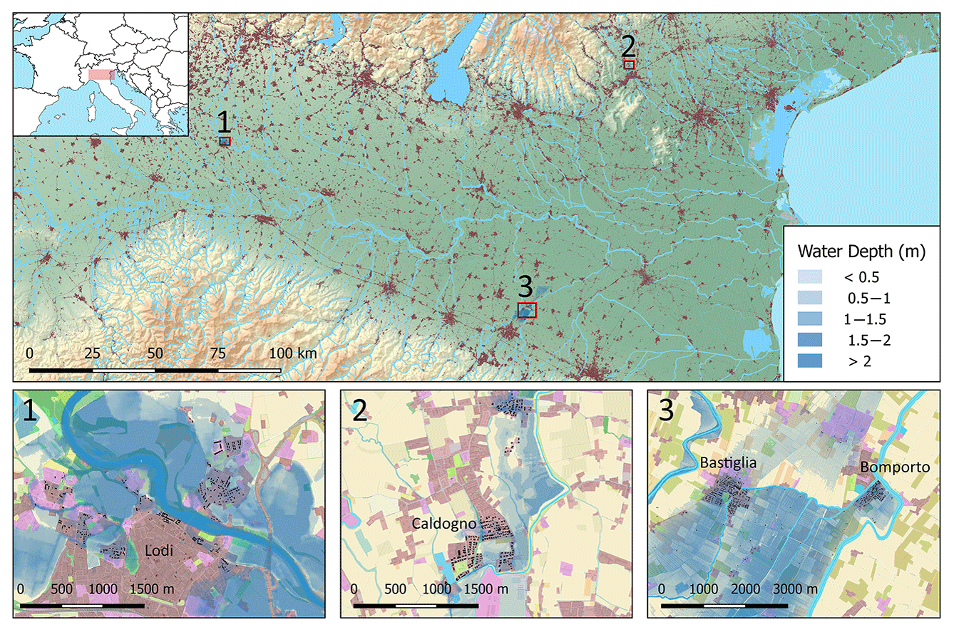
Figure 1Case studies in northern Italy (Po Valley). 1 is Adda River flooding the town of Lodi, 2002; 2 is Bacchiglione River flooding the province of Vicenza, 2010; 3 is Secchia River flooding the province of Modena, 2014. Flooded buildings for which damage records are available are shown in black.
With an area of 46 000 km2, the Po Valley is the largest contiguous floodplain in Italy, extending from the Alps in the north to the Apennines in the south-west and the Adriatic Sea to the east. It comprises the Po River basin, the eastern lowlands of Veneto and Friuli and the south-eastern basins of Emilia–Romagna. The Po Valley is one of the most developed and populated areas in Italy, generating about half of the country's gross domestic product (AdBPo, 2006). In the lower part of the Po River, flood-prone areas are protected by a complex system of embankments and hydraulic works that are part of the flood defence system in the Po Valley, extending for almost 3000 km as a result of a tradition of river embanking lasting centuries (Govi and Turitto, 2000; Lastoria et al., 2006; Masoero et al., 2013). However, flood protection structures generate a false sense of security and low-risk awareness among the floodplain residents (Tobin, 1995). As a result, exposure has steadily increased in flood-prone areas of the Po Valley (Domeneghetti et al., 2015). Records of past flood events (1950–1995) maintained by the National Research Council (Cipolla et al., 1998) show that more than 3300 individual locations were affected by approximately 300 flood events within the Po Valley.
Three of the most recent flood events within the Po Valley (Fig. 1) have been chosen as case studies for this analysis: the 2002 Adda flood that affected the province of Lodi (Lombardy) (1), the 2010 Bacchiglione flood which involved the area of Vicenza (2) and the 2014 Secchia flood in the province of Modena (3). All three locations were subject to frequent flooding between 1950 and 2000, according to the historical catalogue. A short description of these three events is provided hereafter to aid in understanding the dynamics and impacts of each flood.
2.1 Adda 2002
On 27 November 2002, the province of Lodi suffered a flood caused by the overflow of the Adda River. The flood wave reached a record discharge of about 2000 m3 s−1, corresponding to a return period of 100 years (Rossetti et al., 2010). The river overflowed the embankments and first flooded the rural area and then the residential and commercial areas within the capital town of the province, Lodi. The low-speed floodwaters rose to 2.5–3 m. The inundation lasted for about 24 h and affected a large area of the Adda floodplain, including 5.5 ha of residential buildings. No casualties were reported, but several families were evacuated during the emergency and important service nodes, such as hospitals, were severely affected. The reported damage to residential properties, commercial assets and agriculture added up to EUR 17.7 million, of which EUR 7.8 million is related to residential buildings.
2.2 Bacchiglione 2010
From 31 October to 2 November 2010, persistent rainfall affected the pre-Alpine and foothill areas of the Veneto region, exceeding 500 mm in some locations (ARPAV, 2010). As a result, about 140 km2 of land was flooded, involving 130 municipalities (Belcaro et al., 2011). The Bacchiglione River, in the province of Vicenza, was particularly negatively affected. Heavy precipitation events and early snow melting increased the hydrometric levels of the Bacchiglione River and its tributaries, surpassing historical records (Belcaro et al., 2011). On the morning of 1 November, the water flowing at 330 m3 s−1 opened a breach on the right levee of the river, flooding the countryside and the settlements of Caldogno, Cresole and Rettorgole with an average water depth of 0.5 m (ARPAV, 2010). Then the river overflowed downstream towards the city of Vicenza, which was inundated up to its historic centre. The inundation lasted about 48 h and its extent was about 33 ha, 26 ha of which consisted of agricultural land and 7 ha of urban areas. The total damage, including residential properties, economic activities, agriculture and public infrastructures, was estimated to be about EUR 26 million, while dwellings alone accounted for EUR 7.5 million (Scorzini and Frank, 2017).
2.3 Secchia 2014
In January 2014 severe rainfall lasted 2 weeks in the central area of the region of Emilia–Romagna, discharging the annual average amount of rain in just a few days. In the early morning of 19 January, the water started to overflowed a section (10 m) of the of the right levee of the Secchia River, which stands 7–8 m above the floodplain. Later that morning the levee breached at its top by 1 m, flooding the countryside. After 9 h, the entire levee section was destroyed for a length of 80 m, spilling 200 m3 s−1 and flooding about 6000 ha of rural land (D'Alpaos et al., 2014). Seven municipalities were affected, with the small towns of Bastiglia and Bomporto suffering the largest impacts. Both towns, including their industrial districts, remained flooded for more than 48 h. The total volume of water inundating the area was estimated to be about 36 million m3, with an average water depth of 1 m (D'Alpaos et al., 2014). The economic cost inflicted on residential properties, according to damage declaration, amounted to EUR 36 million.
3.1 Data description
We first collected detailed and uniform data portraying hazard and exposure in the areas affected by the three events in order to evaluate their relationship with impacts. Several data sets were compiled from different sources, harmonised and geographically projected to the building level (i.e. micro-scale) for each one of the three study areas. The data set comprises the following:
-
detailed hazard data, including flood extent, depth, duration and flow velocity;
-
high-resolution spatial exposure data, including type, location and value of affected buildings;
-
comprehensive vulnerability data, including the characteristics of buildings and dwellings in terms of material, quality and age;
-
reported damage in terms of replacement and reconstruction costs.
The main hazard features (extent, depth, flow velocity and duration) were obtained from flood maps produced by 2-D hydraulic models based on observations performed during and after the events. In detail, the flood simulation for the Adda River was produced by means of a River2D model (Steffler and Blackburn, 2002) using a 10 m computational mesh based on a high-resolution lidar DEM (Scorzini et al., 2018). The Bacchiglione flood was simulated by using the 1-D–2-D model Infoworks RS (Beta Studio, 2012). The 1-D river network geometry resulted from a topographic survey of cross sections, while the 2-D floodplain morphology (5 m resolution) was obtained from lidar. The reliability of the simulations for the Adda and Bacchiglione floods was verified by using hydrometric data, aerial surveys of inundated areas and photos/videos from the affected population (Rossetti et al., 2010; Scorzini et al., 2018; Scorzini and Frank, 2017). The Secchia flood event was simulated by using an innovative, time-efficient approach (Vacondio et al., 2016), which integrated both river discharge and floodplain characteristics in a parallel computation. The simulation was performed on a 5 m grid and its results were validated against several field data and observations, including a high-resolution radar image (Vacondio et al., 2014, 2017).
The information needed for characterising exposure was collected from a variety of sources and then spatially projected to get a georeferenced data set for each case study. The footprints of buildings were obtained from the OpenStreetMap database (Geofabrik GmbH, 2018) and associated with the official data set of addresses. The land cover was freely available as perimeters classified by the CORINE legend (fourth level of detail) (Feranec and Otahel, 1998) obtained from Regional Environmental Agencies databases. Land cover information was used to distinguish dwellings from other types of buildings (industrial, commercial, etc.). In addition, indicators for building characteristics (Table 1) were selected from the database of the 2011 population census (ISTAT, 2011). Reconstruction and restoration costs per EUR m−2 were obtained for the case study areas from the CRESME database (CRESME/CINEAS/ANIA, 2014). They were used to convert the absolute damage values into relative damage shares. We chose to measure impacts in relative terms so as to make them easier to compare through different times (inflation effect) and places (different currencies). Empirical damage records were gathered from local administrations after the flood events in relation to household street numbers. The records falling outside the simulated flood extents were filtered from the data set. Each record includes claimed, verified and refunded damage to residential buildings. Since actual compensation often covered only a fraction of the damage costs, claimed damage was preferred in order to gauge the economic impact (see Carisi et al., 2018). We restricted our analysis on direct monetary damage to the structures of residential buildings, excluding furniture and vehicles. Economic losses, building values and construction costs for the three events were scaled to 2015 euro inflation values.
3.2 Damage model overview
Empirical damage models are drawn based on actual data collected from specific events (e.g. Luino et al., 2009; Hasanzadeh Nafari et al., 2017); in some regions they represent the only knowledge base for the assessment of flood risk. However, they carry a large uncertainty when employed in different times and places (Gissing and Blong, 2004; McBean et al., 1986). Instead, synthetic models are based on a valuation survey which assesses how the structural components are distributed in the height of a building (Barton et al., 2003; Oliveri and Santoro, 2000; Smith, 1994). In such expert-based models, the magnitude of potential flood loss is estimated based on the vulnerability of structural components via a “what-if” analysis by evaluating the corresponding damage based on building and hazard features (Gissing and Blong, 2004; Merz et al., 2010). Most empirical and synthetic models are UVMs based on water depth as the only predictor of damage, yet recent studies (Dottori et al., 2016; Schröter et al., 2014; Wagenaar et al., 2018) suggest that MVMs developed using expert-based or machine-learning approaches outmatch the performances of customary univariable regression models. However, the development of MVMs requires a comprehensive set of data in order to correctly identify complex relationships among variables. Models can be further classified in relation to the scale of their development and application (de Moel et al., 2015): “micro-scale” usually refers to a model built to account for impacts on individual building components, and it is commonly applied for local assessment; “meso-scale” refers to sub-national analyses, which commonly rely on data aggregated on provincial or regional administrative units; “macro-scale” concerns assessments at national or global level.
3.3 Models from the literature
There are few models in the literature that are dedicated to the economic assessment of flood impacts over Italian residential structures (see e.g. Oliveri and Santoro, 2000; Huizinga, 2007; Luino et al., 2009; Dottori et al., 2016). All such models have been developed independently by using different approaches, assumptions, scale and base data. The first model selected for testing (Luino et al., 2009) is an empirical UVM based on the official impact data collected at micro-scale after the flash-flood event of May 2002 in the Boesio Basin, in Lombardy. One stage-damage curve was generated for structural damage to the most common building type in the area by using loss data measured after the flood, combined with estimates of water depth from an 1-D hydraulic model. In this model, the estimation of building value is based on its geographical location, use and typology, based on market value quotations by the official real estate observatory of Italy (Agenzia delle Entrate, 2018). The second model (OS – Oliveri and Santoro, 2000) is a synthetic UVM developed for a study performed at the micro-scale in the city of Palermo (Sicily). The model describes damage in relation to water depth and consists of two curves, one for two-storey buildings and the other for those taller than two storeys. It considers water stage steps of 0.25 m for each stage, and the model computes the overall replacement cost as the result of damage over different components (internal and external plaster, fixtures, floors and electrical appliances), plus the expenses for dismantling the damaged components. This model is based on an estimate of the average reconstruction value of exposed properties, a hydraulic simulation of potential flood hazard and expert-based assumptions about the damage process, but it has not been validated on empirical damage data. The third model we included in our analysis is part of a stage-damage curve database developed for the meso-scale by the EU Joint Research Centre (Huizinga, 2007; Huizinga et al., 2017) on the basis of an extensive literature survey. Damage curves are provided for a variety of assets and land use classes on the global scale by normalising the maximum damage values in relation to country-specific construction costs. These are obtained by means of statistical regressions with socio-economic development indicators. The JRC curves are suggested for application at the supranational scale but can be a general guide for making assessments at the meso-scale in countries where specific risk models are not available. We selected the curve provided for Italian residential buildings (JRC-IT) to be tested on our data set, although JRC curves have already been tested at the micro-scale in Italy, revealing significant uncertainty in their estimates (Amadio et al., 2016; Carisi et al., 2018; Hasanzadeh Nafari et al., 2017; Scorzini and Frank, 2017).
The fourth model considered is INSYDE, In-depth Synthetic Model for Flood Damage Estimation (Dottori et al. 2016), which is a synthetic MVM developed for residential buildings and released as open-source R script. Repair or replacement costs are modelled by means of analytical functions describing the damage processes for each component as a function of hazard and building characteristics, by using an expert-based “what-if” approach at the micro-scale. Hazard features include physical variables describing the flood event at building location, e.g. water depth, flood duration, presence of contaminants and sediment load.
Indicators related to exposure and vulnerability include building characteristics such as geometry and features. Building features affect cost estimations either by modifying the damage functions or by affecting the unit prices of the building components by a certain factor. Damage categories include clean-up, removal costs and damage to finishing elements such as windows, doors, wirings and installations (Fig. 2). The model adopts probabilistic functions for some of the building components, for which it is difficult to define a deterministic threshold of damage occurrence in relation to hazard parameters. The curves are calibrated on damage micro-data surveyed from a flood event in central Italy (Umbria) (Molinari et al., 2014). Despite the large number of inputs, the model proved to be adaptable to the actual available knowledge of the flood event and building characteristics (Molinari and Scorzini, 2017). The list of explicit inputs accounted for by the INSYDE model is adopted to select the variables accounted for by all MVMs assessed in our analysis (Table 1).
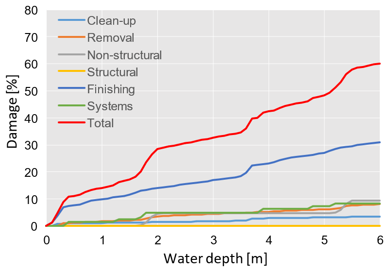
Figure 2Examples of damage curves in relation to water depth produced by INSYDE for riverine floods in relation to a building with FA = 100 m2, NF = 2, BT = 3, BS = 2, FL = 1, YY = 1990 and CS = 1.
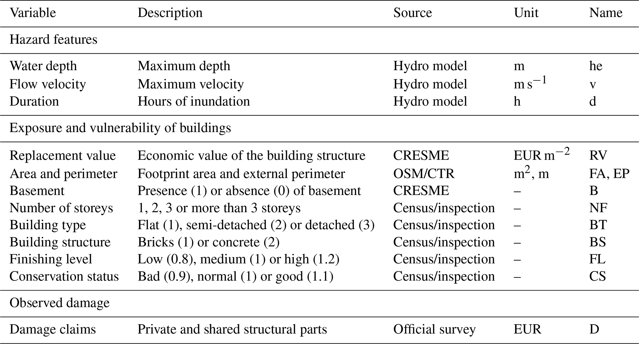
Table 1List of variables included in the multivariable analysis.
3.4 Models trained on observed records
This section provides an overview of the empirical damage models obtained from our events data set, namely two supervised-learning algorithms (random forest, artificial neural network) and three uni- and bivariable regression models used to assess the importance of variables (listed in Table 1) as damage predictors. Trained models share the same sampling approach for validation: the observation data set is split into three parts, two-thirds of which are used to train the model and one-third of which is for validation. This process is iterated 1000 times, scrabbling the data and resampling the training set at each cycle. The output takes the mean of all iterations and provides a curve which represents the empirical damage relationship for the three events. This cross-validation approach had previously been employed in Hasanzadeh Nafari et al. (2017) and in Seifert et al. (2010) in order to optimise the statistical utility of the collected sample.
3.4.1 Multivariable models: supervised-learning algorithms
A probabilistic approach is required in damage estimation in order to control the effects of data variability on the model uncertainty. This is useful for overcoming the limitations associated with the choice of a single model and increasing the statistical value of the analysis (Kreibich et al., 2017). The algorithms we employed to deal with the empirical data share an iterative scrambling and resampling approach (1000 repetitions) in order to draw the confidence interval of the models independently from source data variability. For the set-up of empirically based MVMs we selected 10 variables from those listed in Table 1, excluding those with small variability (basement, conservation status) or those for which an adequate level of detail was not possible to obtain in our case studies. These 10 variables serve as input for two supervised machine-learning algorithms, namely RF and ANN, described in the next paragraphs. Both algorithms were trained on our empirical data set and produced a distribution of estimates for each record, from which the mean value was calculated.
Random forest
The RF is a data mining procedure, a tree-building algorithm that can be used for classification and regression of continuous dependent variables (CART method – see Breiman, 1984), like the one used by Merz et al. (2013). RF has numerous advantages, such as accuracy of prediction, tolerance of outliers and noise, avoidance of overfitting problems and no need to make assumptions about independence, distribution or residual characteristics. Because of this, it has already been employed in the context of natural hazards, including earthquake-induced damage classification (Tesfamariam and Liu, 2010), flood hazard assessment (Wang et al., 2015) and flood risk (Carisi et al., 2018; Chinh et al., 2015; Kreibich et al., 2017; Merz et al., 2013; Spekkers et al., 2014).
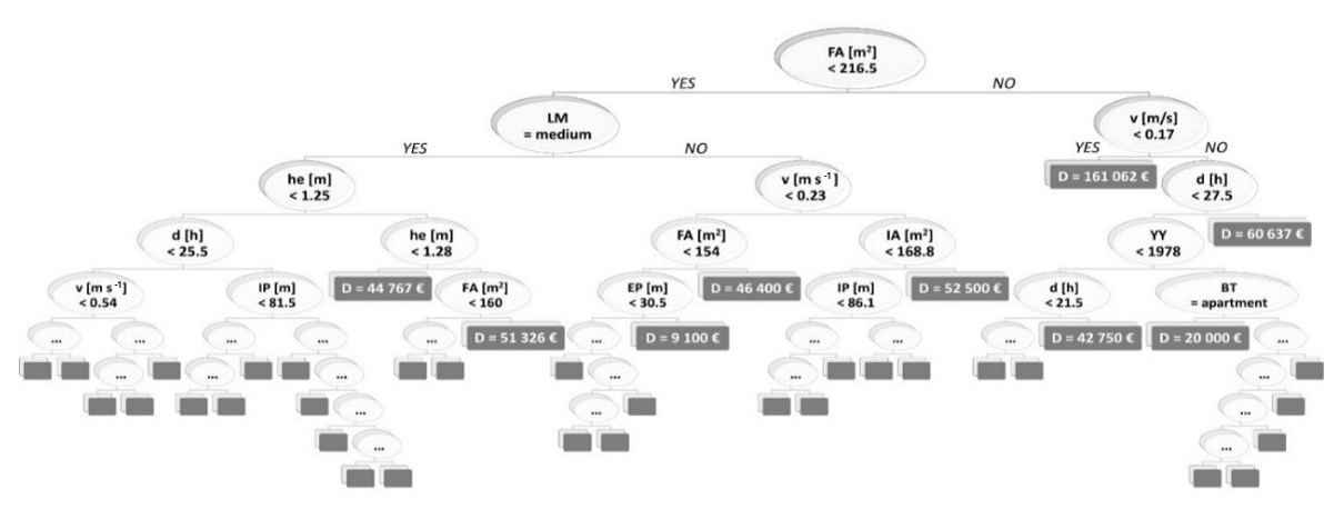
We used the algorithm implemented in the R package RandomForest by Liaw and Wiener (2002). The random forest algorithm builds and combines many decision trees (500 in our case), where each tree has a non-linear regression structure, recursively splitting the input data set into smaller parts by identifying the variables and their splitting values, which maximises the predictive accuracy of the model. The tree structure has several branches, each one starting from the root node and including several leaf nodes, until either a threshold for the minimum number of data points in leaf nodes is reached, or no further splitting is possible (see Liaw and Wiener, 2002 for details about the default values used, e.g. the size of the leaves). The minimum number of observations per leaf is five. Each estimated value represented by the resulting terminal node of the tree answers the partition question asked in the previous interior nodes and depends on the response variable of all the parts of the original data set that are needed to reach the terminal node (Merz et al., 2013). In order to reduce the uncertainty associated with the selection of a single tree, the RF algorithm (Breiman, 2001) creates several bootstrap replicas of the learning data and grows regression trees for each subsample, considering a limited number of variables at each split (normally, this number is equal to the square root of the number of the total variables). This will result in a great number of regression trees, each based on a different (although similar) set of damage records and each leaving out a different number of variables at each split. The mean value among all predictions of the individual trees is chosen as the representative output. An example of a built tree for the present study is shown in Fig. 3. Another important strength of RF is its capability to evaluate the relative importance of each independent variable in the tree-building procedure, i.e. in our case, in representing the damage process. By randomly simulating the absence of one predictor, the RF algorithm calculates the model's performance decrease and thus the importance of the variables in the prediction.
Artificial neural network
ANNs are mathematical models based on non-linear, parallel data processing (Haykin, 2001). They have been applied in several fields of research, such as hydrology, remote sensing and image classification (Campolo et al., 2003; Giacinto and Roli, 2001; Heermann and Khazenie, 1992). The model used in this study (Essenfelder, 2017) consists of a multi-layer perceptron (MLP) neural network model that uses back-propagation as the supervised training technique and the Levenberg–Marquardt as the optimisation algorithm (Hagan and Menhaj, 1994; Yu and Wilamowski, 2011) (see Fig. 4 for the model's structure).

Figure 4Structure of the artificial neural network model applied in this study by using two neuron (node) layers.
The ANN model evaluates the sum of squared errors (SSEs) of the model outputs with regard to the targets for each training epoch, as a way of assessing the generalisation property of a trained ANN model (Hsieh and Tang, 1998; Maier and Dandy, 2000). The ANN runs in a multi-core configuration and as a result provides an ensemble of trained ANN models, thus is suitable for probabilistic analysis. The input and target information are normalised by feature scaling before being processed by the model, while the initial number of hidden neurons per hidden layer is approximated as two-thirds of the summation of the number of neurons in the previous and subsequent layers (Han, 2002). Regarding the activation functions, a log-sigmoid function is used for the connection with neurons in the first and second hidden layers, while a linear function is used for the connections with neurons in the output layer, allowing values to be either lower or greater than the maximum observed value in the target data set. This configuration is interesting, as it does not limit the output range of the ANN model to the range of normalised values. The input data are randomly split between three distinct sets, namely training, validation and test. The training data set is used to calibrate the ANN model, meaning that the weight connections between neurons are updated with respect to the data available in this data set. The learning rate is controlled by coefficient μ: when μ is very small, the training process approximates the Gauss–Newton optimisation algorithm (i.e. fast learning, low stability), while when μ is very large, the training process resembles the steepest descent algorithm (i.e. slow learning, high stability). The value of μ starts as 1 and is updated during each training epoch: μ is reduced by half if the training epoch is successful in reducing the SSE in the output layer; otherwise, the value of μ is increased by a factor of 2 and a new training attempt is performed. The validation set is utilised to avoid the overtraining or overfitting of the ANN model, being used to stop the training process. The test set is not presented to the model during the training procedure, since it is used only as a way of verifying the efficiency of a trained ANN when stressed by new data. In order avoid any possible bias coming from the random split of the original data set into training, validation and test data sets, about 1000 training attempts are performed, each with a different initial weight initialization and training data set composition. The resulting ANN model consists of an ensemble of four models, representing the best overall results after the training procedure, which are used to define the confidence interval.
3.4.2 Univariable and bivariable models
In order to understand if the added complexity of MVMs brings any improvement in the accuracy of damage estimates, we compare them with traditional, deterministic univariable (UVM) and bivariable (BVM) regression models that are empirically derived from the observation data set. Considering the first (water depth) or the first two variables (water depth and flow velocity), we investigate whether a linear, logarithmic or exponential function has the best regression fit to the records. All functions that consider water depth are forced to pass through the origin, because most buildings have no basement and, accordingly, no water means no damage. As we did for the MVM training, we used an iteration of 1000 scrambling and resampling cycles, which were repeated by using the two different sampling strategies: first the models were trained on two-thirds of the data and validated on the remaining one-third of the records.
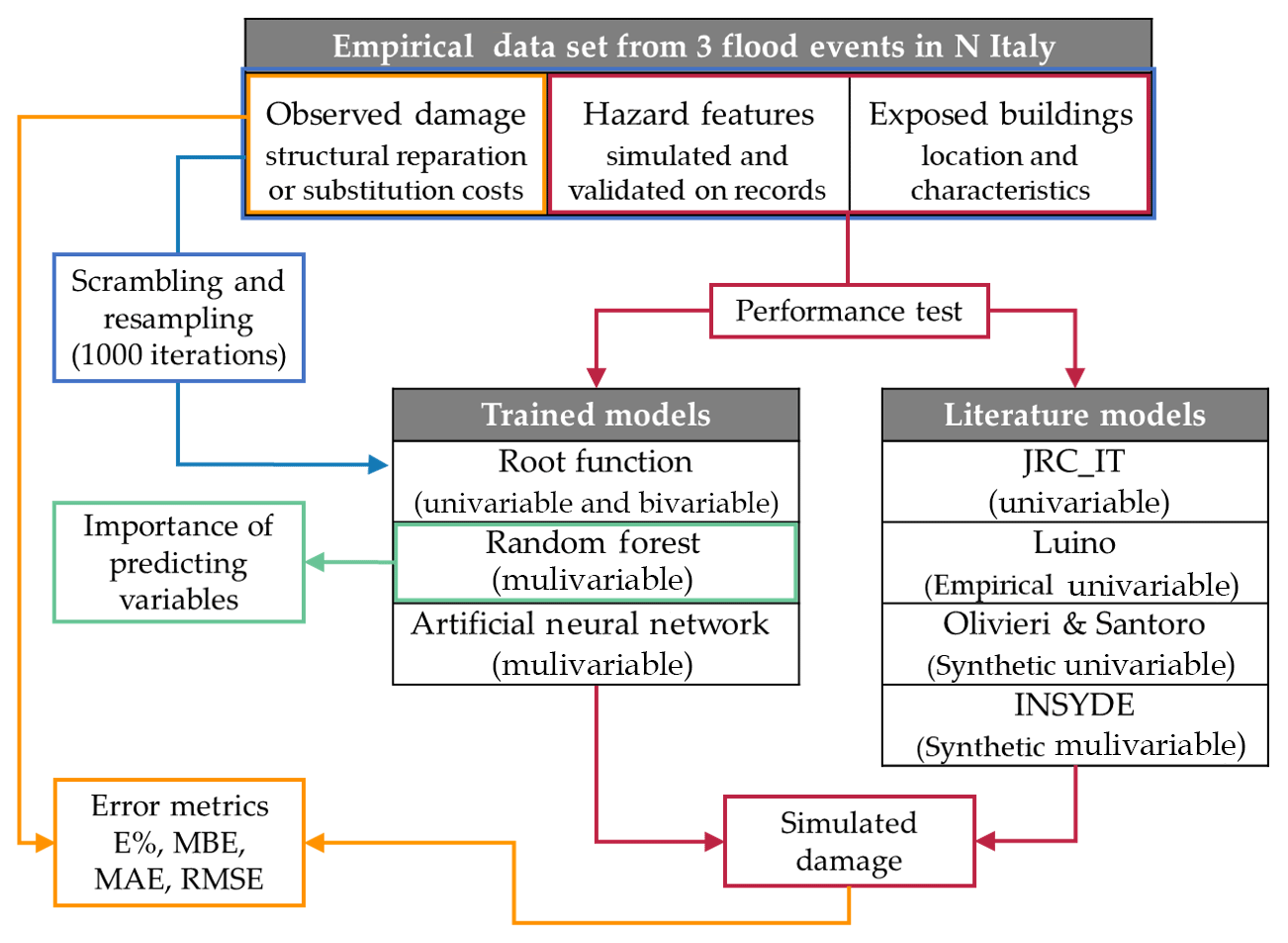
3.4.3 Workflow of the study
The main elements of the study are represented in the workflow shown in Fig. 5. The data set collected from flood events is presented for training the UV, BV and MV models by iterative cross-fold procedure. The trained RF provides the relative importance of predictive variables. Hazard and exposure variables are then used to test the performance of both trained and literature models. Simulated damage is compared to observed costs in terms of error metrics.

4.1 Observed damage records
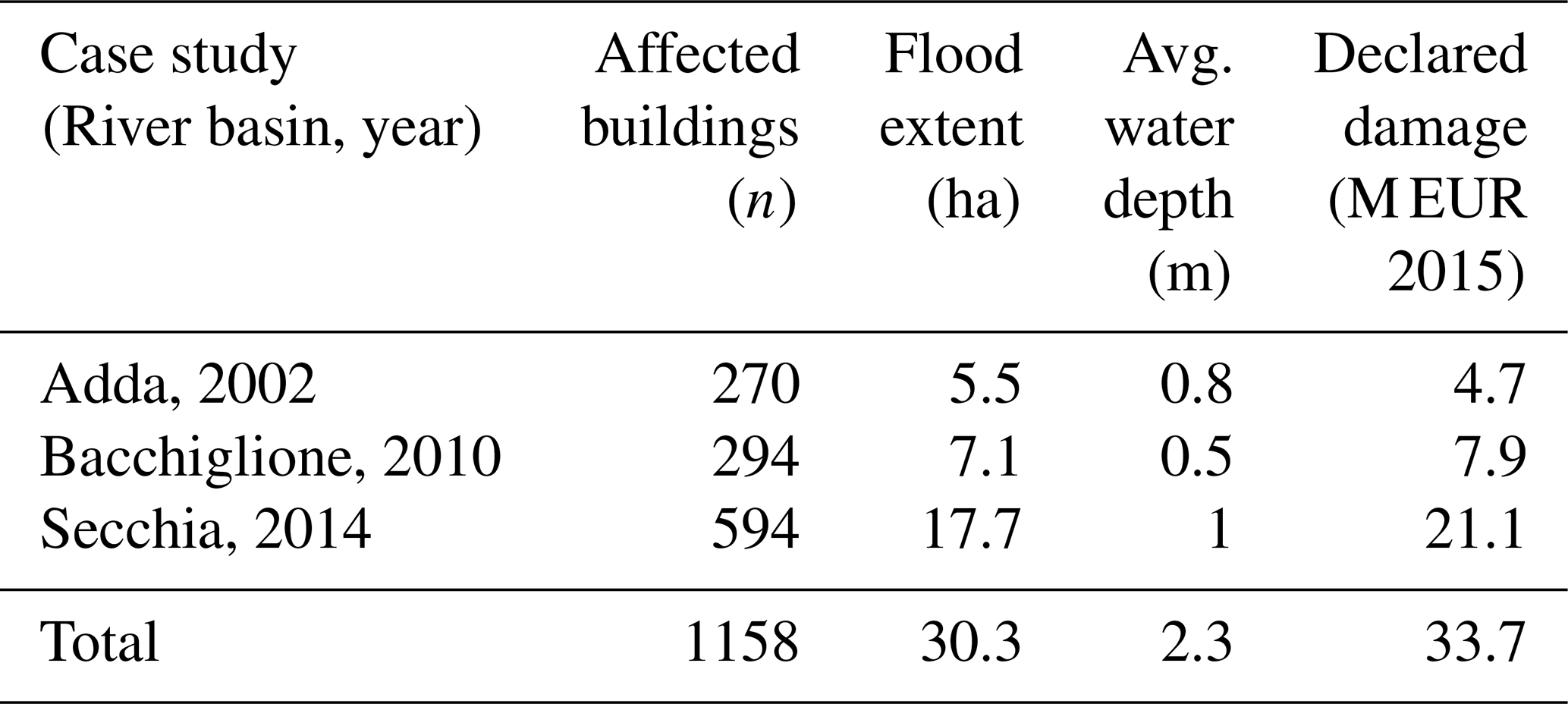
Our combined data set contains records of 1158 damaged residential buildings (Table 2). More than half of these were damaged by the Secchia flood, which affected the largest residential area (17.7 ha) and caused the largest total losses. Only verified, spatially matching records are accounted for; economic losses are scaled to 2015 euro inflation values. Note that these losses are related to the structural damage of residential buildings; thus, they do not represent the full cost inflicted by these events.
Table 2Summary of residential buildings affected by the three investigated flood events, according to hydraulic simulations and damage claims.
Box plots in Fig. 6 show the variance of variables driving the damage. Water depths range from 0.01 to about 2 m, with most records falling in a 0.4–1.2 m interval. Water velocities range between 0.01 and 1.5 m s−1. Footprint areas and observed relative damages have similar average values for all three events; however the Secchia case study presents a longer count of records as well as the largest spread of outliers.
The scatter plot in Fig. 7 better shows the density of observed damage records in relation to the maximum water depth. The increase in depth corresponds to a larger range of variability in economic damage.
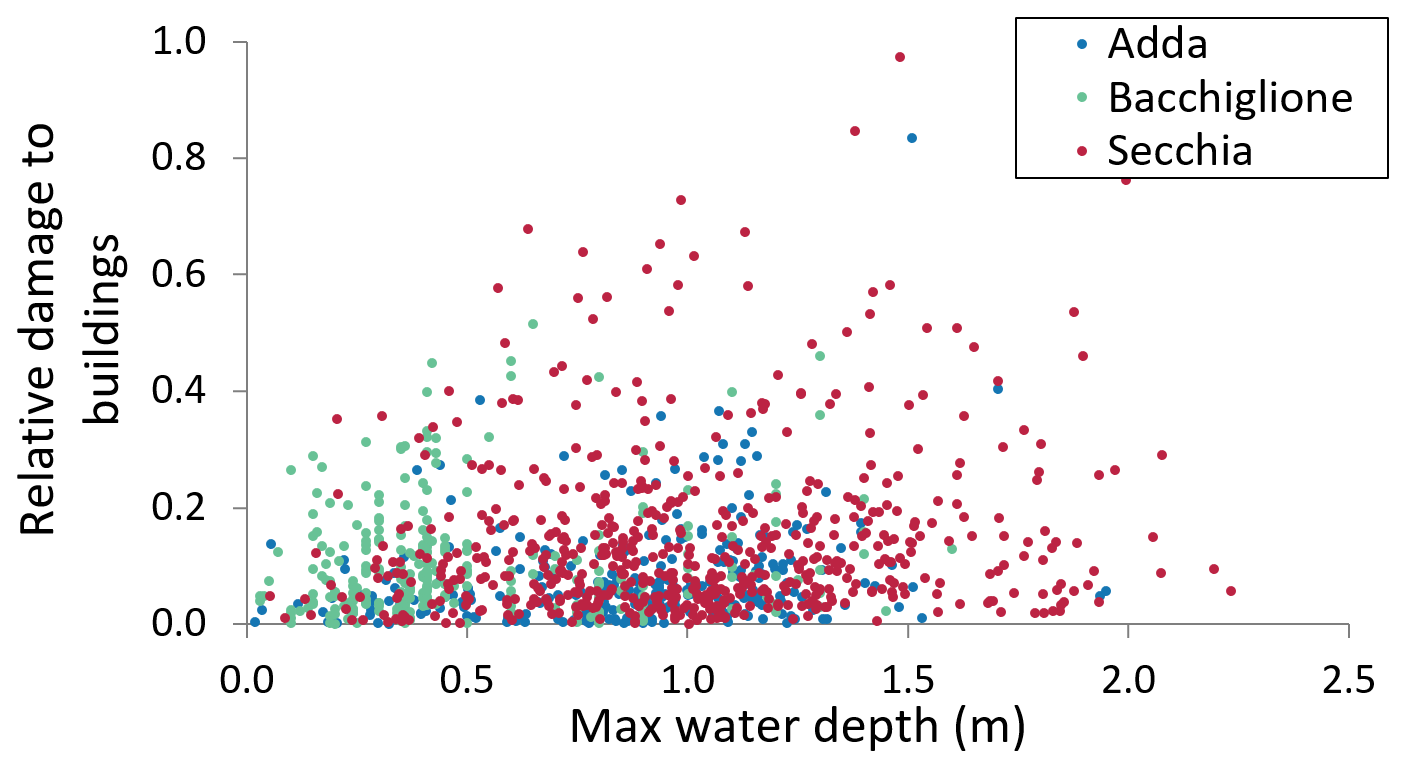
Figure 7Scatter plot of relative damage (y axis) in relation to maximum observed water depth (x axis). Records from the same event are shown with the same colour.
4.2 Influence of hazard and exposure variables on predicting flood damage
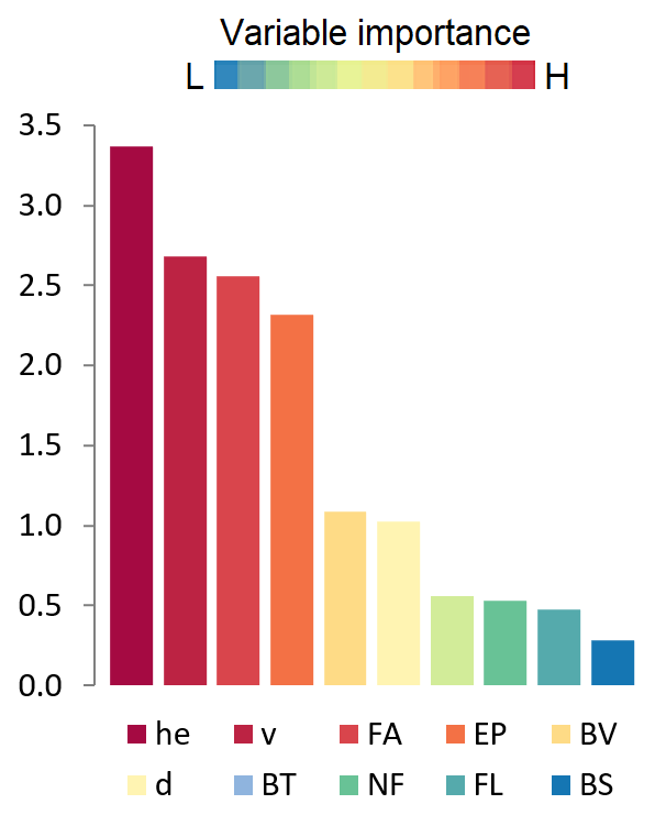
Water depth (he) is identified by RF as the most important predictor of damage (factor 3.4) among the 10 examined variables (Fig. 8). This confirms previous findings (Wagenaar et al., 2017b) and justifies the use of depth-damage curves for post-disaster assessment. Flow velocity and geometric characteristics of buildings (area and perimeters) are also important (factor 2.7 to 2.3), followed by other predictors such as building value, flood duration, number of storeys, finishing level (quality) and type of structure (factor 1 or less). Although water depth is the most influential variable, it is only moderately more important than other predictors. This substantiates efforts to test the applicability of multivariable approaches to improve damage estimation.
4.3 Performance of damage models
To assess the predictive capacity of the four selected literature models, we compare them with empirically based, data-trained models structured on the same variables; i.e. the evaluation of the model performances is carried out by measuring and comparing the error metrics from the aforementioned models (JRC-IT, Luino, OS and INSYDE) to those provided by the empirical MVMs obtained from supervised-learning algorithms, the BVMs and traditional UVMs (depth-damage curves) developed on our data set. The performance of each model is evaluated by using three metrics, namely mean absolute error (MAE), mean bias error (MBE) and root mean square error (RMSE). The MAE indicates the precision of the model in replicating the total recorded damage. The MBE shows the systematic error of the model, which is its mean accuracy. The RMSE measures the average magnitude of the error, enhancing the weight of larger errors. In addition to these error metrics, the total percentage error (E %, difference between observed and simulated damage, divided by observed damage) is shown in the tables.
4.3.1 Literature models
As a first step, estimates of empirical and synthetic models from the literature are compared with observed damages, and the results, in terms of total loss and total percentage error, are shown in Table 3. JRC-IT is the worst-performing model, largely overestimating damage from the three events (E % 143–417). This confirms previous findings about the scarce suitability of JRC meso-scale models for application at the micro-scale, without previous validation (as in Amadio et al., 2016; Carisi et al., 2018; Hasanzadeh Nafari et al., 2017; Scorzini and Frank, 2017). The UV empirical model from Luino overestimates damage with a percentage error ranging from 44 to 177. This probably happens because the damage curve is based on observations from a flash-flood event characterised by higher flow velocities and larger relative impacts, proving that empirical models should be transferred with caution on flood events with characteristics different from those from which the models are generated.
Table 3Estimates and error from literature models compared to observed damage. Monetary values are in M EUR. E % is total percentage error.
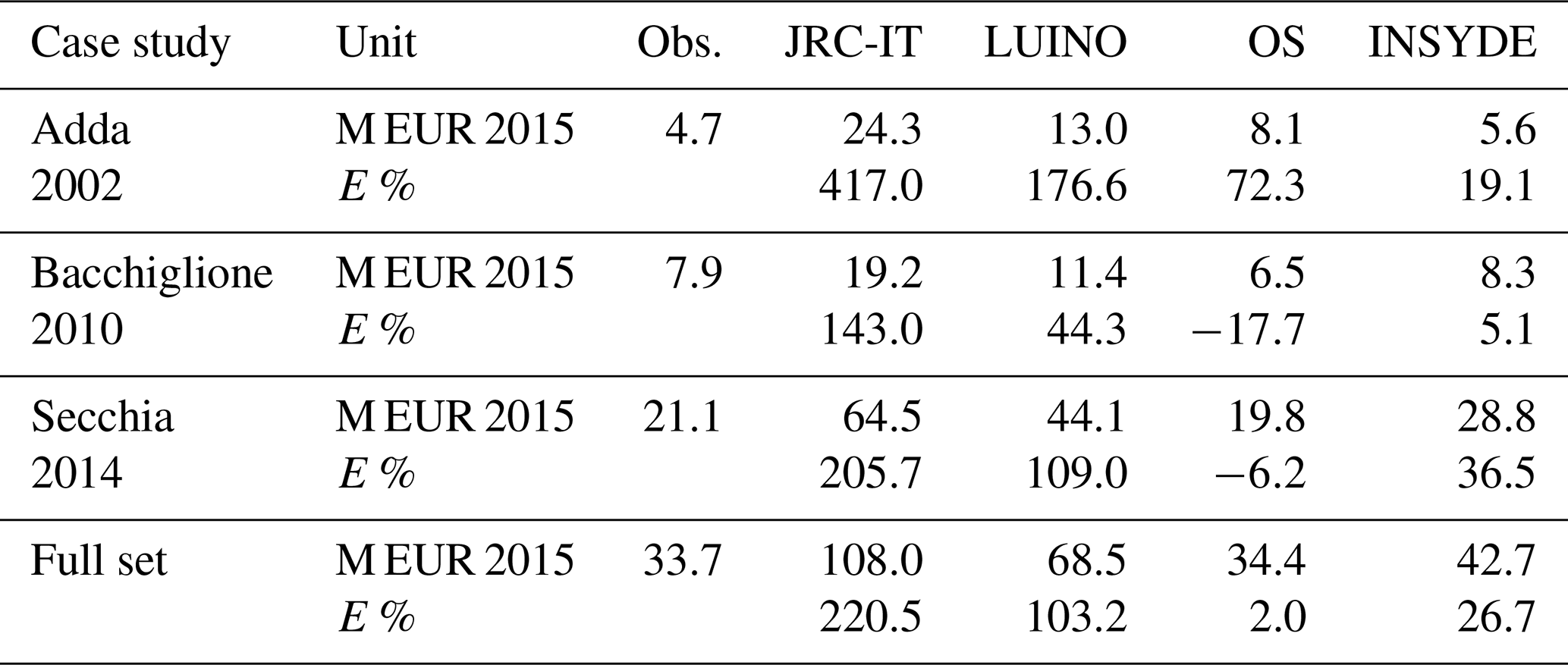
The two synthetic models, OS and INSYDE, perform much better, yet show a large variability of the error factor, depending on the case being considered. In detail, OS provides better results for the Secchia event (6 % underestimation) and worse results for the Adda set (72 % overestimation), resulting in an estimate that is very close to the observations in terms of percentage error of the total data set, although this is mainly due to the compensation of positive and negative errors for the different events. On the contrary, the INSYDE model exhibits a better performance for the Bacchiglione event (5 % overestimation) and a worse one for the Secchia case study (37 % overestimation). Figure 9 compares the estimated and observed damages for the entire data set for the two best-performing literature models (OS and INSYDE).
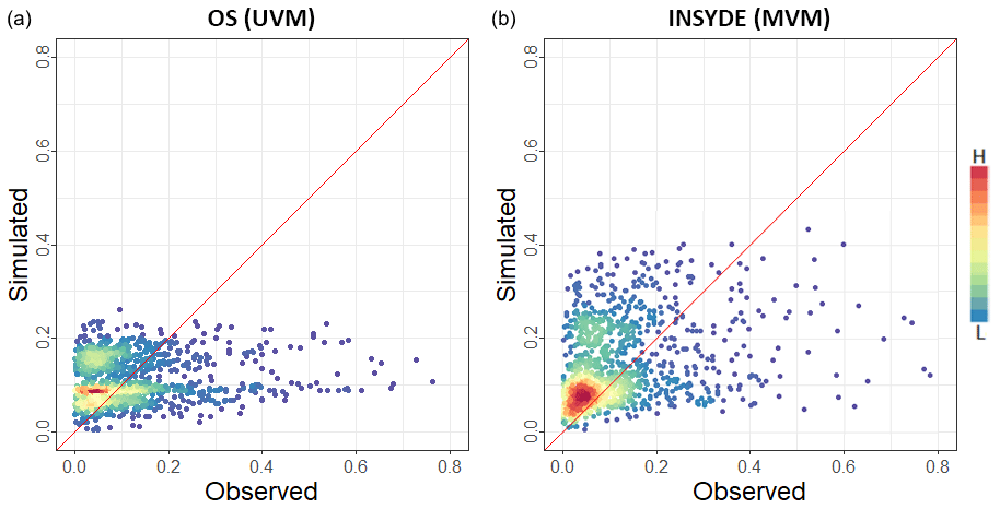
Figure 9Scatter plot comparing relative damage estimates produced by the two best-performing literature models, OS (a) and INSYDE (b). Simulated damage is on the y axis; observed damage is on the x axis. Colours represent record density.
It is worth noting that, although the accuracy of the OS model is higher than that of the INSYDE model for the full set, the latter is more accurate for two out of the three case studies (i.e. Adda 2002 and Bacchiglione 2010). Moreover, the INSYDE model provides more precise results, with an error variance 10 times lower than that of the OS model and with maximum errors never exceeding an absolute value of 40 %. However, INSYDE seems to consistently overestimate the total damages.
4.3.2 Data-trained univariable, bivariable and multivariable models
In this section, damage values estimated by empirical, data-trained UVMs, BVMs and MVMs are compared with observed damage data. The results provided by these empirically based models are used as a benchmark for understanding the capability of tested literature models in predicting damage. The error metrics chosen for comparing the model performances are presented for relative damage based on official estimates of replacement value; however, training and validation were also carried out in terms of monetary damage with similar results, not presented here for the sake of brevity.
The results shown in Table 4 and Fig. 10 indicate no significant differences between UVMs and BVMs. We can affirm that the inclusion of flow velocity as a complementary explanatory variable does not improve the performance of simple regression models in our case study. For this reason, from now on BVMs are dropped from further discussion to focus on a direct comparison between UVMs and MVMs.
Table 4Error metrics for the univariable and bivariable models.
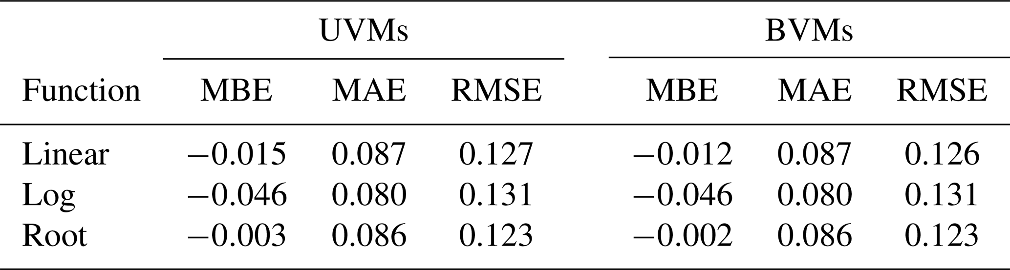
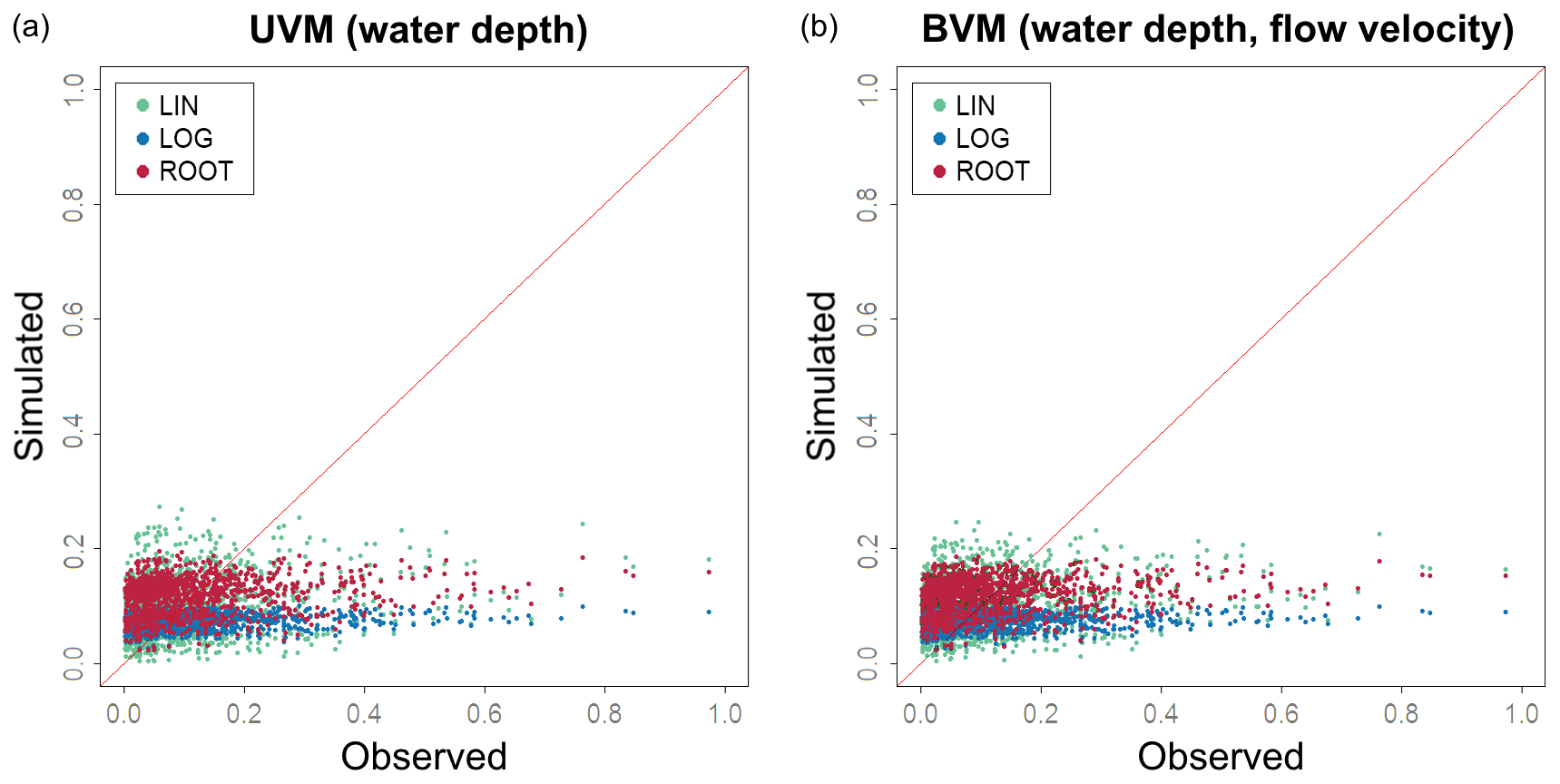
Figure 10Testing the predictive capacity of uni- and bivariable models: estimated relative damage (y axis) from the UVM (a) and BVM (b) are plotted against observed relative damage (x axis), according to the three tested regression functions (LINear, LOGarithmic and ROOT function).
If we take into consideration only UVMs, the MAE and RMSE are very similar for the three tested regression functions. However, the root function described by the general formula has a slightly better fit (correlation is higher, MBE is lower) compared to linear and log functions. We selected the function described by the equation as the best-performing UVM to be included in the comparison with MVMs. Our findings confirmed previous results indicating that the curve shape described by the root function is the most adequate for describing the flood damage process (Buck and Merkel, 1999; Cammerer et al., 2013; Elmer et al., 2010; Kreibich and Thieken, 2008; Penning-Rowsell et al., 2005; Scawthorn et al., 2006; Sluijs et al., 2000; Thieken et al., 2008; Wagenaar et al., 2017b).
Figure 11 shows a direct comparison between the damage estimated by the empirically based models and the observed damage. The upper panel shows the output from the UVM described by the root function. The lower panels show the output of the RF (left) and ANN (right) algorithms. The two machine-learning algorithms produced comparable results, with both RF and ANN models tending to slightly overestimate the average damage (higher density of points, in red) and to significantly underestimate extreme values (lower density of values, in blue). This is a common result of data-driven models, where better results are biased to high-frequency values in comparison to low-frequency values due to the larger sample of those data in the calibration data set. In Fig. 10, the range of estimates, shown as min–max, describes the confidence of the model for individual records. In the case of RF, it shows the min–max range over all the 1000 iterations of the model, while in the case of ANN only an ensemble of the four best-suited models is shown.
Theoretically, MVMs should simulate the complexity of the flooding mechanism better than UVMs. In our test, the ANN model has the best fit to the data, but UVMs (depth-damage curves) appear to perform similarly: the MVMs describe recorded damage with a percentage error of between 0.2 and 10, while the UVM error is about 12 (see Table 5 in the next paragraph). Accordingly, when extensive descriptive data are not available, UVMs appear to be a reasonable alternative for describing the flood damage process. These empirically data-driven models are useful for understanding the capability of multivariable approaches in predicting damage, i.e. which is the range of uncertainty that can be expected when assessing the flood damage process, as compared to simpler models such as UVMs.
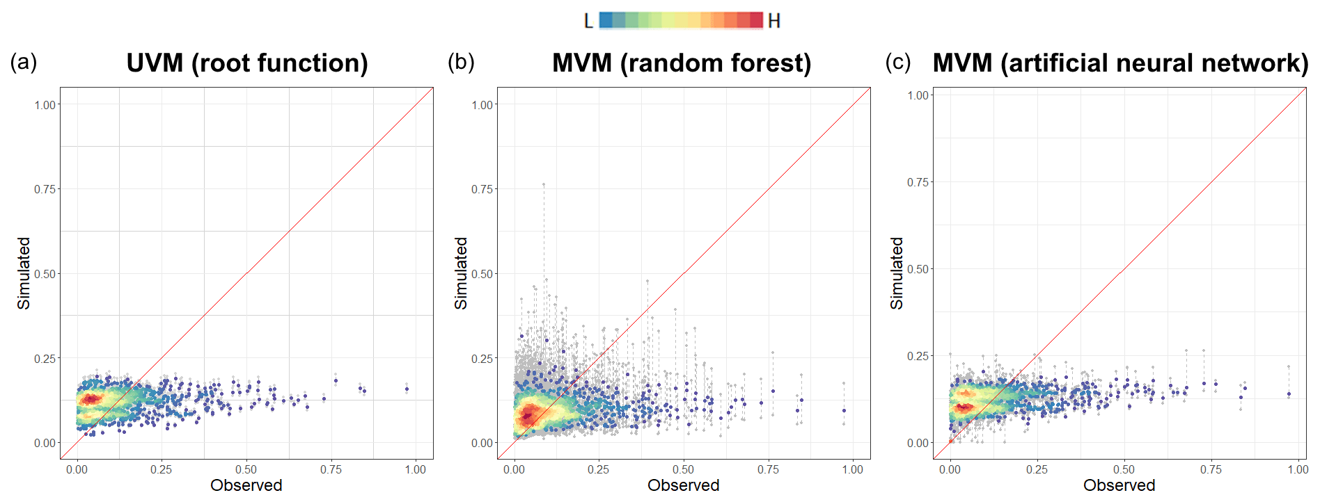
Figure 11Comparison of the predictive capacity of UV and MV models: simulated damage (y axis) is plotted against the observed damage (x axis) for the UV model by using square root function (a), random forest (b) and artificial neural network (c). The grey dashed line shows the range of model outputs for each damage record. The median is shown in colour as a function of the record density.
4.3.3 Comparing model performances
First, we evaluate how selected literature UVMs (JRC-IT, Luino and OS) compare to the root function trained on the empirical data set. Figure 12 shows the distribution and density of observed relative damage as a function of water depth for the full data set, together with the UV curves selected for testing. This figure explains the results presented in Sect. 4.3.1, with the JRC-IT and Luino models growing too fast for shallow water depths, as opposed to OS (shown as two separate curves for different numbers of storeys), which has a good mean fit to the data.
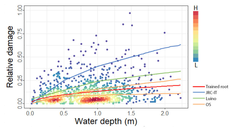
Figure 12Scatter plot of relative damage records (y axis) and water depth (x axis). Point colours represent record densities. The red line shows the empirical root function ()), selected as best suited. The other lines represent the three UV literature models (JRC-IT, Luino and OS) selected for the test. The OS model is made up of two curves in relation to the number of storeys.
Table 5 summarises the main results from all the models in terms of error metrics. Specifically, among all models, MVMs RF and ANN are those with the lowest MAE and RMSE, followed by UVM ROOT with a MAE of 0.086 and an RMSE of 0.123. In terms of percentage error, the ranking is the same, with the sole exception of the OS result, which in terms of this metric lies between the two empirical data-trained MVMs. Overall, the two expert-based literature models, OS and INSYDE, are the best-performing ones when benchmarked against empirically trained models, as shown by the MAE, MBE and RMSE. As mentioned before, the performance of the UVM OS is very close to those of the MVM INSYDE, although this result may depend on the fact that the major share of records comes from the Secchia event, for which OS outperforms INSYDE.
Table 5Comparing error metrics between empirically based models and INSYDE.
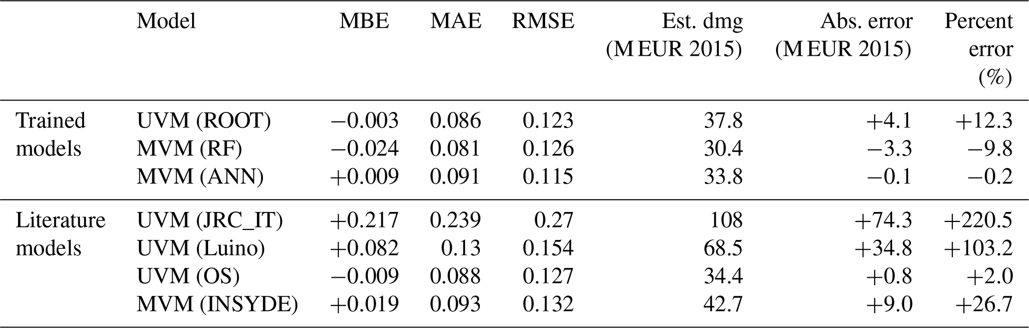
Based on these results, the synthetic models INSYDE and OS currently represent good alternatives for flood risk assessment in Italy, in cases where no empirical loss data are available to develop specific damage models. Indeed, our analysis has shown that particular care should be taken when transferring models derived from specific events (Luino curve) or from different scales (JRC-IT), while synthetic models can be considered more robust tools, relying on a physically based description of flood damage mechanisms. Overall, for the data set investigated, the synthetic MVM INSYDE was found to provide performances not much different from those of the UV OS. However, the results of INSYDE were more precise if we consider the different flood events with a general, although limited, damage overestimation in all the cases, as opposed to OS, which exhibited a more accurate performance only for the Secchia flood and larger variability for the other two events, consequently being less precise. Thus, caution should be used in generalising this finding. Further validation exercises, combined with the application of standardised, detailed procedures for damage data collection (e.g. Molinari et al., 2014) could improve INSYDE's predictive accuracy; since it is an open-source model, the damage functions can be modified for the different building components. For example, the availability of data sets with building losses subdivided into different categories (e.g. structural/non-structural elements, finishing, systems) could help to identify which damage components are responsible for the larger share of the error. The same cannot be said for OS, which is presented as a simple stage-damage curve, without a detailed explanation of the modelling assumptions on the considered flood damage mechanisms.
We cannot exclude that the performances of MVMs would benefit from the inclusion of additional predictive variables, such as those related to the implementation of an early warning system and precaution measures, or social vulnerability; however, the availability of such information is limited for our case study. As a final consideration, the accuracy and precision of damage observations are key factors for the correct development of an MVM. This makes synthetic and empirical MVMs better suited for applications at the micro-scale (up to the census block scale; Molinari and Scorzini, 2017), where explanatory variables can be spatially disaggregated. Indeed, the aggregation scale is of primary importance in the application of MVMs: if we can compare our results to those reported in other studies applying similar multivariable approaches on an extensive damage data set (bagging of regression trees), as in Wagenaar et al. (2017a) and in Kreibich et al (2017), we observe that our range of uncertainty is drastically smaller. This difference is likely imputable to the fact that, in the referred studies, information is aggregated at the municipality level, as opposed to our case, where each variable is precisely linked to the building locations.
Risk management requires a reliable assessment tool to identify priorities in risk mitigation and adaptation. Such a tool should be able to describe potential damage based on the available data related to hazard features and exposure characterisation. Recent studies suggest that multivariable flood damage modelling can outperform customary univariable models (depth-damage functions). In this study we collected a large empirical data set at the micro-scale (i.e. individual buildings), which includes multiple hazard and exposure variables for three riverine flood events in northern Italy, including the declared economic damage to residential buildings. On this basis, we produced three univariable, three bivariable and two multivariable models that are compared in terms of predictive accuracy and precision. We found that water depth is the most important predictor of flood damage for the assessed events, followed by secondary variables related to hazard (flow velocity, duration) and exposure features (area, perimeter and replacement value of the building). However, our results suggest that the inclusion of one additional variable (flow velocity) does not improve the estimates produced by simple regression models in a bivariable set-up. On the other hand, the analysis confirms the literature notion that the root function is the curve best suited for describing damage in relation to water depth. Two MVMs were trained by using two different machine-learning algorithms, namely random forest and artificial neural network. These empirically trained MVMs performed well (with errors ranging from 1 % to 10 %) in reproducing the damage output from the three events and thus were set as a reference for assessments in the same geographical context. In this perspective, other case studies are needed to confirm their robustness. Moreover, our results corroborate previous findings about the advantages of supervised machine-learning approaches for developing or improving flood damage models. Still, their application remains limited by the availability of the data required for the MVM set-up. However, in the case of a scarce number of variables, simple univariable models trained on the specific contexts seem to be a good alternative to MVMs.
We then considered four literature models of different natures and complexities to be tested on our extended case study data set. We compared their error metrics with those of the empirically trained UVMs and MVMs in order to evaluate their performance as a predictive tool for flood risk assessment. The results showed important errors when transferring models derived from different countries and scales, such as the JRC-IT curve, or from events with different characteristics, such as the empirical model from Luino, which is based on a flash-flood event in which flow velocity likely has a significant role in flood impacts. On the other hand, we found that both UV (Oliveri and Santoro, 2000) and MV (INSYDE, Dottori et al., 2016) synthetic models can provide similar results (although with larger uncertainties) to those observed from the empirically trained models. The tested synthetic models can be currently considered as the best option for damage prediction purposes in the Italian context, in cases where no extensive loss data are available to derive a location-specific flood damage model. Overall, we found that errors produced by synthetic models were within 30 % of observed damage, with MVM INSYDE providing more precise results over the single case study events (with a percentage overestimation of 19 %, 5 % and 37 % of observed damage for Adda, Bacchiglione and Secchia, respectively) and is more accurate for two out of the three case studies (i.e. Adda and Bacchiglione), while the OS model is generally less precise but more accurate for the sole Secchia flood event (2 % error, as opposed to a 72 % overestimation for the Adda and an 18 % underestimation for the Bacchiglione event).
Observed errors depend in part on the inherent larger variability found in the data set related to that particular event. Nevertheless, the collection of additional independent flood records from different geographical contexts in Italy would help to further evaluate the adaptability of these models, estimate their uncertainty and increase their predictive accuracy. The open-source INSYDE model holds the best potential in this sense. To conclude, the work presented here has assembled a data set that is currently one of the most extensive and advanced for Italy: empirical damage data are the most important set of information for improving and validating damage models. On this track, we aim to promote a shared effort towards an updated catalogue of floods that includes hazard, exposure and damage information at the micro-scale. To this end, the adoption of a standardised and detailed procedure for damage data collection is a mandatory step.
The data set developed for this research is available upon request to the author. The INSYDE model is available as an R open-source code from https://github.com/ruipcfig/insyde (Dottori et al., 2016). The hazard simulation of the Secchia flood event was kindly provided by Renato Vacondio (University of Parma), who we sincerely thank.
MA, AS, FC designed the study, provided the data, produced the analysis and wrote the manuscript. AHE contributed with the analysis performed using the artificial neural network. AHE, AD, JM and AC helped with the interpretation of results and the critical revision of the article. All authors reviewed the final manuscript.
The authors declare that they have no conflict of interest.
This article is part of the special issue “Flood risk assessment and management”. It is a result of the EGU General Assembly 2018, Vienna, Austria, 8–13 April 2018.
The research leading to this paper received funding through the projects CLARA (EU's Horizon 2020 research and innovation programme under grant agreement no. 730482) and SAFERPLACES (Climate-KIC innovation partnership).
The authors express their gratitude to Daniela Molinari, who provided the data for the Adda case study, within the framework of the Flood-Impat+ project, funded by Fondazione Cariplo.
This paper was edited by Cristina Prieto and reviewed by two anonymous referees.
AdBPo: Caratteristiche del bacino del fiume Po e primo esame dell'impatto ambientale delle attività umane sulle risorse idriche, Autorità di Bacino del Fiume Po, Po River Basin Authority, available at: ahttp://adbpo.gov.it/ (last access: 21 March 2019), 2006.
Agenzia delle Entrate: Osservatorio del Mercato Immobiliare – Quotazioni zone OMI, available at: http://www.agenziaentrate.gov.it/wps/content/Nsilib/Nsi/Documentazione/omi/Banche+dati/Quotazioni+immobiliari/ (last access: 1 July 2015), 2018.
Alfieri, L., Feyen, L., Salamon, P., Thielen, J., Bianchi, A., Dottori, F., and Burek, P.: Modelling the socio-economic impact of river floods in Europe, Nat. Hazards Earth Syst. Sci., 16, 1401–1411, https://doi.org/10.5194/nhess-16-1401-2016, 2016.
Amadio, M., Mysiak, J., Carrera, L., and Koks, E.: Improving flood damage assessment models in Italy, Nat. Hazards, 82, 2075–2088, https://doi.org/10.1007/s11069-016-2286-0, 2016.
ANIA – Associazione Nazionale fra le Imprese Assicuratrici: Le alluvioni e la protezione delle abitazioni, available at: http://www.ania.it/it/index.html (last access: 21 March 2019), 2015.
Apel, H., Thieken, A. H., Merz, B., and Blöschl, G.: Flood risk assessment and associated uncertainty, Nat. Hazards Earth Syst. Sci., 4, 295–308, https://doi.org/10.5194/nhess-4-295-2004, 2004.
Apel, H., Aronica, G. T., Kreibich, H., and Thieken, A. H.: Flood risk analyses – how detailed do we need to be?, Nat. Hazards, 49, 79–98, https://doi.org/10.1007/s11069-008-9277-8, 2009.
ARPAV: Scheda Evento “Idro” 31 Ottobre–5 Novembre 2010, available at: w http://www.regione.veneto.it/web/guest;jsessionid=A6A80F62BAA03DE9D8F9AB8D629441FA.liferay01 (last access: 21 March 2019), 2010.
Barton, C., Viney, E., Heinrich, L., and Turnley, M.: The Reality of Determining Urban Flood Damages, in: NSW Floodplain Management Authorities Annual Conference, Sydney, 2003.
Belcaro, P., Gasparini, D., and Baldessari, M.: 31 ottobre–2 novembre 2010: l'alluvione dei Santi, Regione Veneto, available at: http://statistica.regione.veneto.it/ (last access: 21 March 2019), 2011.
Beta Studio: Interventi per la sicurezza idraulica dell'area metropolitana di Vicenza: bacino di laminazione lungo il Torrente Timonchio in comune di Caldogno – Progetto definitivo, Relazione idrologica e idraulica, Regione Veneto, available at: http://statistica.regione.veneto.it/ (last access: 21 March 2019), 2012.
Breiman, L.: Classification and regression trees, Chapman & Hall, available at: https://books.google.it/books/about/Classification_and_Regression_Trees.html?id=JwQx-WOmSyQC&redir_esc=y (last access: 30 July 2018), 1984.
Breiman, L.: Random Forests, Mach. Learn., 45, 5–32, https://doi.org/10.1023/A:1010933404324, 2001.
Buck, W. and Merkel, U.: Auswertung der HOWASSchadendatenbank, Institut für Wasserwirtschaft und Kulturtechnik der Universität Karlsruhe, Karlsruhe, 1999.
Cammerer, H., Thieken, A. H., and Lammel, J.: Adaptability and transferability of flood loss functions in residential areas, Nat. Hazards Earth Syst. Sci., 13, 3063–3081, https://doi.org/10.5194/nhess-13-3063-2013, 2013.
Campolo, M., Soldati, A., and Andreussi, P.: Artificial neural network approach to flood forecasting in the River Arno, Hydrolog. Sci. J., 48, 381–398, https://doi.org/10.1623/hysj.48.3.381.45286, 2003.
Carisi, F., Schröter, K., Domeneghetti, A., Kreibich, H., and Castellarin, A.: Development and assessment of uni- and multivariable flood loss models for Emilia-Romagna (Italy), Nat. Hazards Earth Syst. Sci., 18, 2057–2079, https://doi.org/10.5194/nhess-18-2057-2018, 2018.
Carrera, L., Standardi, G., Bosello, F., and Mysiak, J.: Assessing direct and indirect economic impacts of a flood event through the integration of spatial and computable general equilibrium modelling, Environ. Model. Softw., 63, 109–122, https://doi.org/10.1016/j.envsoft.2014.09.016, 2015.
Chinh, D., Gain, A., Dung, N., Haase, D., and Kreibich, H.: Multi-Variate Analyses of Flood Loss in Can Tho City, Mekong Delta, Water, 8, 6, https://doi.org/10.3390/w8010006, 2015.
Cipolla, F., Guzzetti, F., Lolli, O., Pagliacci, S., Sebastiani, C., and Siccardi, F.: Catalogo delle località colpite da frane e da inondazioni: verso un utilizzo più maturo dell'informazione, in: Il rischio idrogeologico e la difesa del suolo, Accademia dei Lincei, 1–2 October 1998, Roma, 285–290, 1998.
CRESME/CINEAS/ANIA: Definizione dei costi di (ri)costruzione nell'edilizia, edited by CINEAS, available at: http://cresme.cineas.it/ (last access: 21 March 2019), 2014.
D'Alpaos, L., Brath, A., and Fioravante, V.: Relazione tecnico-scientifica sulle cause del collasso dell' argine del fiume Secchia avvenuto il giorno 19 gennaio 2014 presso la frazione San Matteo, available at: http://www.comune.bastiglia.mo.it/ (last access: 21 March 2019), 2014.
de Moel, H. and Aerts, J. C. J. H.: Effect of uncertainty in land use, damage models and inundation depth on flood damage estimates, Nat. Hazards, 58, 407–425, https://doi.org/10.1007/s11069-010-9675-6, 2011.
de Moel, H., Jongman, B., Kreibich, H., Merz, B., Penning-Rowsell, E., and Ward, P. J.: Flood risk assessments at different spatial scales, Mitig. Adapt. Strateg. Global Change, 20, 865–890, https://doi.org/10.1007/s11027-015-9654-z, 2015.
Domeneghetti, A., Carisi, F., Castellarin, A., and Brath, A.: Evolution of flood risk over large areas: Quantitative assessment for the Po river, J. Hydrol., 527, 809–823, https://doi.org/10.1016/j.jhydrol.2015.05.043, 2015.
Dottori, F., Figueiredo, R., Martina, M. L. V., Molinari, D., and Scorzini, A. R.: INSYDE: A synthetic, probabilistic flood damage model based on explicit cost analysis, Nat. Hazards Earth Syst. Sci., 16, 2577–2591, https://doi.org/10.5194/nhess-16-2577-2016, 2016.
EASAC: Extreme weather events in Europe, Preparing for climate change adaptation: an update on EASAC's 2013 study, available at: https://easac.eu/publications/ (last access: 21 March 2019), 2018.
EEA – European Environment Agency: Mapping the impacts of recent natural disasters and technological accidents in Europe – An overview of the last decade, available at: https://www.eea.europa.eu/publications#c7=en&c11=5&c14=&c12=&b_start=0 (last access: 21 March 2019), 2010.
EEA: Flood risks and environmental vulnerability – Exploring the synergies between floodplain restoration, water policies and thematic policies, https://doi.org/10.2800/039463, 2016.
Elmer, F., Thieken, A. H., Pech, I., and Kreibich, H.: Influence of flood frequency on residential building losses, Nat. Hazards Earth Syst. Sci., 10, 2145–2159, https://doi.org/10.5194/nhess-10-2145-2010, 2010.
Essenfelder, A. H.: Climate Change and Watershed Planning: Understanding the Related Impacts and Risks, Universita' Ca' Foscari Venezia, Venezia, 2017.
Feranec, J. and Otahel, J. Final version of the 4th level CORINE land cover classes at scale 1 : 50,000, Technical report, European Agency Phaee Topic Link on Land Cover and Institute of Geography, Slovak Academy of Science (SAS), Bratislava, 1998.
Figueiredo, R., Schröter, K., Weiss-Motz, A., Martina, M. L. V., and Kreibich, H.: Multi-model ensembles for assessment of flood losses and associated uncertainty, Nat. Hazards Earth Syst. Sci., 18, 1297–1314, https://doi.org/10.5194/nhess-18-1297-2018, 2018.
Geofabrik GmbH: OpenStreetMap data extracts, available at: http://download.geofabrik.de/ (last access: 30 March 2017), 2018.
Giacinto, G. and Roli, F.: Design of effective neural network ensembles for image classification purposes, Image Vis. Comput., 19, 699–707, https://doi.org/10.1016/S0262-8856(01)00045-2, 2001.
Gissing, A. and Blong, R.: Accounting for variability in commercial flood damage estimation, Aust. Geogr., 35, 209–222, https://doi.org/10.1080/0004918042000249511, 2004.
Govi, M. and Turitto, O.: Casistica storica sui processi d'interazione delle correnti di piena del Po con arginature e con elementi morfotopografici del territorio adiacente, Sci. e vita nel momento attuale, V, 105–160, 2000.
Hagan, M. T. and Menhaj, M. B.: Training Feedforward Networks with the Marquardt Algorithm, IEEE Trans. Neural Networks, 5, 989–993, 1994.
Hallegatte, S.: An adaptive regional input-output model and its application to the assessment of the economic cost of Katrina, Risk Anal., 28, 779–799, https://doi.org/10.1111/j.1539-6924.2008.01046.x, 2008.
Han, J.: Application of Artificial Neural Networks for Flood Warning Systems, North Carolina State University, available at: https://repository.lib.ncsu.edu/handle/1840.16/4173 (last access: 21 March 2019), 2002.
Hasanzadeh Nafari, R., Amadio, M., Ngo, T., and Mysiak, J.: Flood loss modelling with FLF-IT: a new flood loss function for Italian residential structures, Nat. Hazards Earth Syst. Sci., 17, 1047–1059, https://doi.org/10.5194/nhess-17-1047-2017, 2017.
Haykin, S.: Neural Networks: A Comprehensive Foundation, 2nd Edd., Prentice Hall, Inc., Upper Saddle River, NJ, USA, 2001.
Heermann, P. D. and Khazenie, N.: Classification of multispectral remote sensing data using a back-propagation neural network, IEEE T. Geosci. Remote., 30, 81–88, 1992.
Hsieh, W. W. and Tang, B.: Applying Neural Network Models to Prediction and Data Analysis in Meteorology and Oceanography, B. Am. Meteorol. Soc., 79, 1855–1870, https://doi.org/10.1175/1520-0477(1998)079<1855:ANNMTP>2.0.CO;2, 1998.
Huizinga, J.: Flood damage functions for EU member states, Technical report implemented in the framework of the contract # 382441-F1SC awarded by the European Commission – Joint Research Centre, HKV Consultants, Lelystad, 2007.
Huizinga, J., De Moel, H., and Szewczyk, W.: Methodology and the database with guidelines Global flood depth-damage functions, Publications Office of the European Union, ISSN: 1831-9424, https://doi.org/10.2760/16510, 2017.
ISTAT: 15∘ censimento della populazione e delle abitazioni, Istituto nazionale di statistica, Rome, 2011.
Jongman, B., Kreibich, H., Apel, H., Barredo, J. I., Bates, P. D., Feyen, L., Gericke, A., Neal, J., Aerts, J. C. J. H., and Ward, P. J.: Comparative flood damage model assessment: Towards a European approach, Nat. Hazards Earth Syst. Sci., 12, 3733–3752, https://doi.org/10.5194/nhess-12-3733-2012, 2012.
Jonkman, S. N., Bočkarjova, M., Kok, M., and Bernardini, P.: Integrated hydrodynamic and economic modelling of flood damage in the Netherlands, Ecol. Econ., 66, 77–90, https://doi.org/10.1016/j.ecolecon.2007.12.022, 2008.
Koks, E. E., Carrera, L., Jonkeren, O., Aerts, J. C. J. H., Husby, T. G., Thissen, M., Standardi, G., and Mysiak, J.: Regional disaster impact analysis: comparing input–output and computable general equilibrium models, Nat. Hazards Earth Syst. Sci., 16, 1911–1924, https://doi.org/10.5194/nhess-16-1911-2016, 2016.
Kreibich, H. and Thieken, A. H.: Assessment of damage caused by high groundwater inundation, Water Resour. Res., 44, 1–14, https://doi.org/10.1029/2007WR006621, 2008.
Kreibich, H., Thieken, A. H., Petrow, T., Müller, M., and Merz, B.: Flood loss reduction of private households due to building precautionary measures – lessons learned from the Elbe flood in August 2002, Nat. Hazards Earth Syst. Sci., 5, 117–126, https://doi.org/10.5194/nhess-5-117-2005, 2005.
Kreibich, H., Piroth, K., Seifert, I., Maiwald, H., Kunert, U., Schwarz, J., Merz, B., and Thieken, a. H.: Is flow velocity a significant parameter in flood damage modelling?, Nat. Hazards Earth Syst. Sci., 9, 1679–1692, https://doi.org/10.5194/nhess-9-1679-2009, 2009.
Kreibich, H., Botto, A., Merz, B., and Schröter, K.: Probabilistic, Multivariable Flood Loss Modeling on the Mesoscale with BT-FLEMO, Risk Anal., 37, 774–787, https://doi.org/10.1111/risa.12650, 2017.
Lastoria, B., Simonetti, M. R., Casaioli, M., Mariani, S., and Monacelli, G.: Socio-economic impacts of major floods in Italy from 1951 to 2003, Adv. Geosci., 7, 223–229, https://doi.org/10.5194/adgeo-7-223-2006, 2006.
Liaw, A. and Wiener, M.: Classification and Regression by randomForest, R News, 2, available at: https://cran.r-project.org/doc/Rnews/ (last access: 21 March 2019), 2002.
Luino, F., Cirio, C. G., Biddoccu, M., Agangi, A., Giulietto, W., Godone, F., and Nigrelli, G.: Application of a model to the evaluation of flood damage, Geoinformatica, 13, 339–353, https://doi.org/10.1007/s10707-008-0070-3, 2009.
Maier, H. R. and Dandy, G. C.: Neural networks for the prediction and forecasting of water resources variables: A review of modelling issues and applications, Environ. Model. Softw., 15, 101–124, https://doi.org/10.1016/S1364-8152(99)00007-9, 2000.
Masoero, A., Claps, P., Asselman, N. E. M., Mosselman, E., and Di Baldassarre, G.: Reconstruction and analysis of the Po River inundation of 1951, Hydrol. Process., 27, 1341–1348, https://doi.org/10.1002/hyp.9558, 2013.
McBean, E., Fortin, M., and Gorrie, J.: A critical analysis of residential flood damage estimation curves, Can. J. Civ. Eng., 13, 86–94, https://doi.org/10.1139/l86-012, 1986.
Merz, B., Kreibich, H., Thieken, A., and Schmidtke, R.: Estimation uncertainty of direct monetary flood damage to buildings, Nat. Hazards Earth Syst. Sci., 4, 153–163, https://doi.org/10.5194/nhess-4-153-2004, 2004.
Merz, B., Kreibich, H., Schwarze, R., and Thieken, A.: Review article “assessment of economic flood damage,” Nat. Hazards Earth Syst. Sci., 10, 1697–1724, https://doi.org/10.5194/nhess-10-1697-2010, 2010.
Merz, B., Kreibich, H., and Lall, U.: Multi-variate flood damage assessment: a tree-based data-mining approach, Nat. Hazards Earth Syst. Sci., 13, 53–64, https://doi.org/10.5194/nhess-13-53-2013, 2013.
Messner, F., Penning-rowsell, E., Green, C., Tunstall, S., Van Der Veen, A., Tapsell, S., Wilson, T., Krywkow, J., Logtmeijer, C., Fernández-bilbao, A., Geurts, P., and Haase, D.: Evaluating flood damages: guidance and recommendations on principles and methods, FLOODsite Project Deliverable D9.1, Contract No. GOCE-CT-2004-505420, 189, 2007.
Meyer, V. and Messner, F.: National flood damage evaluation methods: A review of applied methods in England, the Netherlands, the Czech republic and Germany, UFZ Discussion Papers 21/2005, Helmholtz Centre for Environmental Research (UFZ), Division of Social Sciences (ÖKUS), 49 pp., 2005.
Molinari, D. and Scorzini, A. R.: On the influence of Input data quality to flood damage estimation: the performance of the INSYDE model, Water, 9, 688, https://doi.org/10.3390/w9090688, 2017.
Molinari, D., Menoni, S., Aronica, G. T., Ballio, F., Berni, N., Pandolfo, C., Stelluti, M. and Minucci, G.: Ex post damage assessment: an Italian experience, Nat. Hazards Earth Syst. Sci., 14, 901–916, https://doi.org/10.5194/nhess-14-901-2014, 2014.
Molinari, D., De Bruijn, K. M., Castillo-Rodríguez, J. T., Aronica, G. T., and Bouwer, L. M.: Validation of flood risk models: Current practice and possible improvements, Int. J. Disast. Risk Reduct., 33, 441–448, https://doi.org/10.1016/j.ijdrr.2018.10.022, 2019.
Mysiak, J., Testella, F., Bonaiuto, M., Carrus, G., De Dominicis, S., Cancellieri, U. G., Firus, K., and Grifoni, P.: Flood risk management in Italy: Challenges and opportunities for the implementation of the EU Floods Directive (2007/60/EC), Nat. Hazards Earth Syst. Sci., 13, 2883–2890, https://doi.org/10.5194/nhess-13-2883-2013, 2013.
Mysiak, J., Surminski, S., Thieken, A., Mechler, R., and Aerts, J.: Brief communication: Sendai framework for disaster risk reduction – success or warning sign for Paris?, Nat. Hazards Earth Syst. Sci., 16, 2189–2193, https://doi.org/10.5194/nhess-16-2189-2016, 2016.
Oliveri, E. and Santoro, M.: Estimation of urban structural flood damages: the case study of Palermo, Urban Water, 2, 223–234, https://doi.org/10.1016/S1462-0758(00)00062-5, 2000.
Paprotny, D., Sebastian, A., Morales-Nápoles, O., and Jonkman, S. N.: Trends in flood losses in Europe over the past 150 years, Nat. Commun., 9, 1985, https://doi.org/10.1038/s41467-018-04253-1, 2018.
Penning-Rowsell, E., Johnson, C., Tunstall, S., Morris, J., Chatterton, J., Green, C., Koussela, K., and Fernandez-bilbao, A.: The Benefits of Flood and Coastal Risk Management: a Handbook of Assessment Techniques, Middlesex Univ. Press, Middlesex, Hydraulic Engineering Reports, ISBN 1904750516, 2005.
Pistrika, A. K. and Jonkman, S. N.: Damage to residential buildings due to flooding of New Orleans after hurricane Katrina, Nat. Hazards, 54, 413–434, https://doi.org/10.1007/s11069-009-9476-y, 2010.
Rossetti, S., Cella, O. W., and Lodigiani, V.: Studio idrologico-idraulico del tratto di F. Adda inserito nel territorio comunale di Lodi, Milano, Studio Paoletti Ingegneri Associati, Milano, 2010.
Scawthorn, C., Flores, P., Blais, N., Seligson, H., Tate, E., Chang, S., Mifflin, E., Thomas, W., Murphy, J., Jones, C., and Lawrence, M.: HAZUS-MH Flood Loss Estimation Methodology. II. Damage and Loss Assessment, Nat. Hazards Rev., 7, 72–81, https://doi.org/10.1061/(ASCE)1527-6988(2006)7:2(72), 2006.
Schröter, K., Kreibich, H., Vogel, K., Riggelsen, C., Scherbaum, F., and Merz, B.: How useful are complex flood damage models?, Water Resour. Res., 50, 3378–3395, https://doi.org/10.1002/2013WR014396. Received, 2014.
Scorzini, A., Radice, A., and Molinari, D.: A New Tool to Estimate Inundation Depths by Spatial Interpolation (RAPIDE): Design, Application and Impact on Quantitative Assessment of Flood Damages, Water, 10, 1805, https://doi.org/10.3390/w10121805, 2018.
Scorzini, A. R. and Frank, E.: Flood damage curves: new insights from the 2010 flood in Veneto, Italy, J. Flood Risk Manage., 10, 381–392, https://doi.org/10.1111/jfr3.12163, 2017.
Scorzini, A. R. and Leopardi, M.: River basin planning: from qualitative to quantitative flood risk assessment: the case of Abruzzo Region (central Italy), Nat. Hazards, 88, 71–93, https://doi.org/10.1007/s11069-017-2857-8, 2017.
Seifert, I., Kreibich, H., Merz, B., and Thieken, A. H.: Application and validation of FLEMOcs – a flood-loss estimation model for the commercial sector, Hydrolog. Sci. J., 55, 1315–1324, https://doi.org/10.1080/02626667.2010.536440, 2010.
Sluijs, L., Snuverink, M., van den Berg, K., and Wiertz, A.: Schadecurves industrie ten gevolge van overstroming, Tebodin Consultant, RWS DWW, Den Haag, 2000.
Smith, D.: Flood damage estimation. A review of urban stage-damage curves and loss function, Water SA, 20, 231–238, 1994.
Spekkers, M. H., Kok, M., Clemens, F. H. L. R., and ten Veldhuis, J. A. E.: Decision-tree analysis of factors influencing rainfall-related building structure and content damage, Nat. Hazards Earth Syst. Sci., 14, 2531–2547, https://doi.org/10.5194/nhess-14-2531-2014, 2014.
Steffler, P. and Blackburn, J.: River2D – Two-dimensional depth averaged model of river hydrodynamics and fish habitat, Cumulative Environmental Management Association, Fort McMurray, CA, 2002.
Tesfamariam, S. and Liu, Z.: Earthquake induced damage classification for reinforced concrete buildings, Struct. Saf., 32, 154–164, https://doi.org/10.1016/j.strusafe.2009.10.002, 2010.
Thieken, A. H., Müller, M., Kreibich, H., and Merz, B.: Flood damage and influencing factors: New insights from the August 2002 flood in Germany, Water Resour. Res., 41, 1–16, https://doi.org/10.1029/2005WR004177, 2005.
Thieken, A. H., Olschewski, A., Kreibich, H., Kobach, S., and Merz, B.: Development and evaluation of FLEMOps – a new Flood Loss Estimation MOdel for the private sector, Flood Recover. Innov. Response, WIT Press, Southampton, UK, 315–324, 2008.
Thieken, A. H., Ackermann, V., Elmer, F., Kreibich, H., Kuhlmann, B., Kunert, U., Maiwald, H., Merz, B., Müller, M., Piroth, K., Schwarz, J., Schwarze, R., Seifert, I., and Seifert, J.: Methods for the evaluation of direct and indirect flood losses, in: RIMAX Contrib. 4th Int. Symp. Flood Def., 6–8 May 2008, Toronto, CA, 1–10, 2009.
Tobin, G. A.: The levee love affair: a stormy relationship?, J. Am. Water Resour. Assoc., 31, 359–367, https://doi.org/10.1111/j.1752-1688.1995.tb04025.x, 1995.
Vacondio, R., Dal Palù, A., and Mignosa, P.: GPU-enhanced finite volume shallow water solver for fast flood simulations, Environ. Model. Softw., 57, 60–75, https://doi.org/10.1016/j.envsoft.2014.02.003, 2014.
Vacondio, R., Aureli, F., Ferrari, A., Mignosa, P., and Dal Palù, A.: Simulation of the January 2014 flood on the Secchia River using a fast and high-resolution 2D parallel shallow-water numerical scheme, Nat. Hazards, 80, 103–125, https://doi.org/10.1007/s11069-015-1959-4, 2016.
Vacondio, R., Dal Palù, A., Ferrari, A., Mignosa, P., Aureli, F., and Dazzi, S.: A non-uniform efficient grid type for GPU-parallel Shallow Water Equations models, Environ. Model. Softw., 88, 119–137, https://doi.org/10.1016/J.ENVSOFT.2016.11.012, 2017.
Van Ootegem, L., Verhofstadt, E., Van Herck, K., and Creten, T.: Multivariate pluvial flood damage models, Environ. Impact Assess. Rev., 54, 91–100, https://doi.org/10.1016/j.eiar.2015.05.005, 2015.
Vogel, K., Riggelsen, C., Scherbaum, F., Schroeter, K., Kreibich, H., and Merz, B.: Challenges for Bayesian Network Learning in a Flood Damage Assessment Application, in: 11th International Conference on Structural Safety & Reliability, 16–20 June 2013, CRC Press, New York, USA, 3123–3130, 2013.
Wagenaar, D., de Jong, J., and Bouwer, L. M.: Data-mining for multi-variable flood damage modelling with limited data, Nat. Hazards Earth Syst. Sci. Discuss., https://doi.org/10.5194/nhess-2017-7, in review, 2017a.
Wagenaar, D., de Jong, J. and Bouwer, L. M.: Multi-variable flood damage modelling with limited data using supervised learning approaches, Nat. Hazards Earth Syst. Sci., 17, 1683–1696, https://doi.org/10.5194/nhess-17-1683-2017, 2017b.
Wagenaar, D., Lüdtke, S., Schröter, K., Bouwer, L. M., and Kreibich, H.: Regional and Temporal Transferability of Multivariable Flood Damage Models, Water Resour. Res., 54, 3688–3703, https://doi.org/10.1029/2017WR022233, 2018.
Wagenaar, D. J., De Bruijn, K. M., Bouwer, L. M., and De Moel, H.: Uncertainty in flood damage estimates and its potential effect on investment decisions, Nat. Hazards Earth Syst. Sci., 16, 1–14, https://doi.org/10.5194/nhess-16-1-2016, 2016.
Wang, Z., Lai, C., Chen, X., Yang, B., Zhao, S., and Bai, X.: Flood hazard risk assessment model based on random forest, J. Hydrol., 527, 1130–1141, https://doi.org/10.1016/j.jhydrol.2015.06.008, 2015.
Yu, H. and Wilamowski, B. M.: Levenberg-Marquardt Training, Intell. Syst., 5, 12–18, https://doi.org/10.1201/b10604-15, 2011.
Zampetti, G., Ottaviani, F., and Minutolo, A.: I costi del rischio idrogeologico, Dossier Legambiente, Roma, 2012.
Zhou, Q., Panduro, T. E., Thorsen, B. J., and Arnbjerg-Nielsen, K.: Verification of flood damage modelling using insurance data, Water Sci. Technol., 68, 425–432, https://doi.org/10.2166/wst.2013.268, 2013.