Projected intensification of sub-daily and daily rainfall extremes in convection-permitting climate model simulations over North America: implications for future intensity–duration–frequency curves

Convection-permitting climate models have been recommended for use in projecting future changes in local-scale, short-duration rainfall extremes that are of the greatest relevance to engineering and infrastructure design, e.g., as commonly summarized in intensity–duration–frequency (IDF) curves. Based on thermodynamic arguments, it is expected that rainfall extremes will become more intense in the future. Recent evidence also suggests that shorter-duration extremes may intensify more than longer durations and that changes may depend on event rarity. Based on these general trends, will IDF curves shift upward and steepen under global warming? Will long-return-period extremes experience greater intensification than more common events? Projected changes in IDF curve characteristics are assessed based on sub-daily and daily outputs from historical and late 21st century pseudo-global-warming convection-permitting climate model simulations over North America. To make more efficient use of the short model integrations, a parsimonious generalized extreme value simple scaling (GEVSS) model is used to estimate historical and future IDF curves (1 to 24 h durations). Simulated historical sub-daily rainfall extremes are first evaluated against in situ observations and compared with two high-resolution observationally constrained gridded products. The climate model performs well, matching or exceeding performance of the gridded datasets. Next, inferences about future changes in GEVSS parameters are made using a Bayesian false discovery rate approach. Large portions of the domain experience significant increases in GEVSS location (>99 % of grid points), scale (>88 %), and scaling exponent (>39 %) parameters, whereas almost no significant decreases are projected to occur (<1 %, <5 %, and <5 % respectively). The result is that IDF curves tend to shift upward (increases in location and scale), and, with the exception of the eastern US, steepen (increases in scaling exponent), which leads to the largest increases in return levels for short-duration extremes. The projected increase in the GEVSS scaling exponent calls into question stationarity assumptions that form the basis for existing IDF curve projections that rely exclusively on simulations at the daily timescale. When changes in return levels are scaled according to local temperature change, median scaling rates, e.g., for the 10-year return level, are consistent with the Clausius–Clapeyron (CC) relation at 1 to 6 h durations, with sub-CC scaling at longer durations and modest super-CC scaling at sub-hourly durations. Further, spatially coherent but small increases in dispersion – the ratio of scale and location parameters – of the GEVSS distribution are found over more than half of the domain, providing some evidence for return period dependence of future changes in extreme rainfall.

1 Introduction

The design of some civil infrastructure – culverts, storm drains, sewers, bridges, etc. – is based on information about local flood extremes with specified low annual probabilities of occurrence (or, equivalently, long return periods). When gauged streamflow data are not available, information about rainfall extremes can instead be used by engineers to infer flood magnitudes for the return periods of interest. The necessary information on the frequency of occurrence, duration, and intensity of rainstorms is compactly summarized in rainfall intensity–duration–frequency (IDF) curves, and hence IDF curves are a key source of information for water resource and engineering design applications (Canadian Standards Association, 2012). Typical IDF curves summarize the relationship between the intensity and occurrence frequency of extreme rainfall over averaging durations ranging from minutes to a day, usually at local gauging sites. Sub-daily and daily rainfall extremes found in IDF curves are also featured in building codes (e.g., 15 min and 1 day of extreme rainfall is used to estimate roof drainage and loading; National Research Council, 2015).

For the purpose of water resource management and engineering design, it has been stated that “stationarity is dead” (Milly et al., 2008). Increases in atmospheric moisture are expected with anthropogenic global warming as saturation vapour pressure – loosely, the moisture holding capacity of the atmosphere – scales approximately exponentially with temperature following the Clausius–Clapeyron (CC) relation (∼7 % ^∘C⁻¹). In the absence of other influences, e.g., changes in large-scale circulation and soil moisture availability, the intensity of extreme rainfall should therefore also increase as the atmosphere warms (Trenberth, 2011). While historical increases in local extreme rainfall are difficult to detect due to the relatively small forced signal relative to natural variability, as well as uncertainties due to measurement errors and series length, evidence from observations over large regions and from climate model simulations is largely consistent with widespread thermodynamically driven intensification of rainfall extremes (Min et al., 2011; Westra et al., 2013a; Zhang et al., 2013; Pfahl et al., 2017). Moving into the future, even with aggressive mitigation strategies, warming will likely continue over typical design lifetimes due to continued emissions of short- and long-lived greenhouse gases and climate forcing agents (Millar et al., 2017). Attendant changes in rainfall extremes are thus also expected to persist with continued warming.

The reality of climate change, in combination with the long service life of infrastructure, has prompted the incorporation of future climate projections into the engineering design process. Despite the general expectation that short-duration rainfall extremes will become more intense in the future, there is still substantial uncertainty about the sensitivity of local rainfall extremes to warming (Westra et al., 2014; Pendergrass, 2018). For example, evidence from some idealized convection-permitting model experiments suggests that sub-daily extremes may intensify more than longer durations (O'Gorman, 2015), but the conditions under which this occurs (e.g., sensitivity to microphysics parameterization) are not fully understood. Furthermore, results from CMIP5 global climate models (GCMs) indicate that rarer extreme daily precipitation events intensify more than less rare events (Kharin et al., 2018), with some indication of return period dependence in sub-daily convection-permitting simulations over small midlatitude domains as well (e.g., Evans and Argueso, 2015; Kuo et al., 2015; Tabari et al., 2016). What will this mean for future IDF curves in North America? Will they shift upward and steepen and will changes in risk depend on return period?

Complicating the transfer of information from climate model simulations to future IDF curves is the historical reliance on (1) climate models with parameterized convection and (2) extrapolation of information on simulated daily extremes to sub-daily extremes. In the first case, short-duration, local-scale rainfall extremes are mostly generated by convective storm systems that are not resolved by most climate models (e.g., those with parameterized convection). Credible projections of localized sub-daily extreme rainfall may require high-resolution convection-permitting climate models (Kendon et al., 2017) in which the convective parameterization scheme is turned off and the model is capable of simulating convective clouds explicitly (Prein et al., 2015). In the second case, prior unavailability of short-duration precipitation outputs from climate models has meant that observed relationships between long and short durations have been used to extrapolate changes at the daily timescale to sub-daily timescales. For instance, Srivastav et al. (2014) used equidistant quantile mapping to statistically downscale and temporally disaggregate daily global climate model outputs to IDF curves at station locations. Assuming a stationary relationship between durations necessarily constrains relative changes in shorter-duration extremes to largely match those at longer durations.

Direct investigation of sub-daily rainfall extremes, and hence IDF curves, from convection-permitting climate models may therefore provide an avenue forward for the water resource management and engineering community. However, integrations of such computationally expensive models are typically short, at most between 1 to 2 decades, which makes robust estimation of rare extremes difficult; the high computational expense has also limited their application to small domains. Zhang et al. (2017) suggested that the use of convection-permitting models, in combination with advanced statistical methods that make better use of short records, may be required to reliably project future changes in short-duration rainfall extremes. Based on this recommendation, the current study links projected changes in sub-daily rainfall extremes from a convection-permitting climate model with changes in specific characteristics of IDF curves using a parsimonious statistical model. Unlike previous studies, which have focused on relatively small domains and/or very short integrations (e.g., Evans and Argueso, 2015; Kuo et al., 2015; Tabari et al., 2016), the focus here is on decadal simulations for a continental domain covering most of North America. The main goals of the study are to (1) assess whether there is evidence for a shift upward and steepening of IDF curves under global warming, (2) determine whether changes depend on return period, and finally (3) link projected changes in IDF curve return levels to the magnitude of local warming.

To this end, hourly 4 km rainfall outputs from historical and end-of-century pseudo-global-warming convection-permitting simulations by the Weather Research and Forecasting (WRF) model (Rasmussen et al., 2017; Liu et al., 2017) are used in conjunction with a parsimonious generalized extreme value simple scaling (GEVSS) model (Nguyen et al., 1998; Van de Vyver, 2015; Blanchet et al., 2016; Mélèse et al., 2018) to estimate historical and future IDF curves (1 to 24 h durations) over a domain covering northern Mexico, the conterminous US, and southern Canada. The pseudo-global-warming simulation perturbs historical boundary conditions with the climate change signal obtained from an ensemble of global climate models. The GEVSS model leverages information from multiple durations to characterize relationships between the frequency of occurrence and duration of extreme rainfall intensities. Assuming that the underlying model assumptions are met, “borrowing strength” by pooling data from different durations provides more robust estimates of GEV distribution parameters than standard un-pooled estimates (Innocenti et al., 2017). Furthermore, the GEVSS model parameterization provides a straightforward framework to make inferences about future changes in IDF curve characteristics. For example, projected increases in the GEVSS temporal scaling exponent lead to greater intensification of shorter-duration extremes relative to longer durations, whereas increases in the dispersion of the GEVSS distribution lead to greater intensification of long-return-period extremes relative to shorter return periods. Statistical model assumptions and simulated historical sub-daily rainfall extremes are evaluated using two high-resolution gridded observational products and in situ station observations. Projected changes in GEVSS parameters, and hence IDF curve characteristics, are obtained under a Bayesian framework, with inferences made using a false discovery rate (FDR) approach to multiple comparisons. Finally, return level projections are expressed as relative changes with respect to local warming – so-called “temperature scaling” – to assess adherence to the theoretical CC relation.

The remainder of the paper is structured as follows. Observational data and model simulations are described in Sect. 2. The GEVSS approach to IDF curve estimation is provided in Sect. 3 and the Bayesian framework for parameter inference is summarized in Sect. 4. Simulated short-duration rainfall extremes and goodness of fit of the GEVSS model are evaluated in Sect. 5. Projected changes in GEVSS parameters and IDF curves are summarized in Sect. 6 along with estimates of temperature scaling of extreme rainfall return levels. Finally, Sect. 7 provides a discussion of results, conclusions, and suggestions for future research.

2 Observations and simulations

Climate model simulations and observational data used in this study are summarized in Table 1. To investigate future changes in extreme short-duration rainfall and associated IDF curves over North America, precipitation outputs from convection-permitting climate model simulations performed by the National Center for Atmospheric Research (NCAR) using WRF model version 3.4.1 (Liu et al., 2017; Rasmussen et al., 2017) are used at their 1 h archived time step. Outputs from two sets of WRF simulations – a historical control run (CTRL) and a pseudo-global-warming (PGW) simulation for the end of the 21st century – each on the same 1360×1016 4 km grid, are provided over a domain (referred to as HRCONUS) spanning northern Mexico, the conterminous US, and southern Canada (Fig. 1). In both cases, spectral nudging of geopotential height, horizontal wind, and temperature (five model layers above the top of the boundary layer) is applied at spatial scales greater than ∼2000 km and with an e-folding time of ∼6 h. Boundary conditions for the CTRL simulation are given by the European Centre for Medium-Range Weather Forecasts ERA-Interim reanalysis (Dee et al., 2011) for the period from 1 October 2000 to 30 September 2013. The PGW simulation uses the same ERA-Interim boundary conditions, but with all variables perturbed with the climate change signal from an ensemble of Coupled Model Intercomparison Project Phase 5 (CMIP5) (Taylor et al., 2012) global climate models taken between 1976 and 2005 and between 2071 and 2100 under the Representative Concentration Pathway (RCP8.5) scenario (Meinshausen et al., 2011).

Importantly, the experimental design – including PGW and spectral nudging – suppresses the influence of internal variability, which would otherwise make detection of forced changes more difficult. It is thus mainly able to isolate the thermodynamic climate change response over the domain. While vertical temperature structure and baroclinicity can be modified by the PGW perturbation, substantive changes in large-scale circulation are not considered (Liu et al., 2017; Prein et al., 2017c). However, decomposition of the forced response of daily-scale extreme rainfall in CMIP5 models into thermodynamic and dynamic components suggests that the dynamic contribution over Canada and the US is small (Pfahl et al., 2017). Furthermore, by focusing on the late 21st century and RCP8.5 forcings, the PGW experiment is exposed to a relatively large warming signal relative to the CTRL simulation (global mean temperature change of +3.5 ^∘C), which will also tend to enhance detectability of local-scale changes. Further details on the simulations are provided by Liu et al. (2017) and Rasmussen et al. (2017).

ECCC (2014)Xie et al. (2017)Beck et al. (2017a, b)Liu et al. (2017)Liu et al. (2017)Rasmussen et al. (2017)

Table 1 Summary of observational data and climate model simulations used in the study.

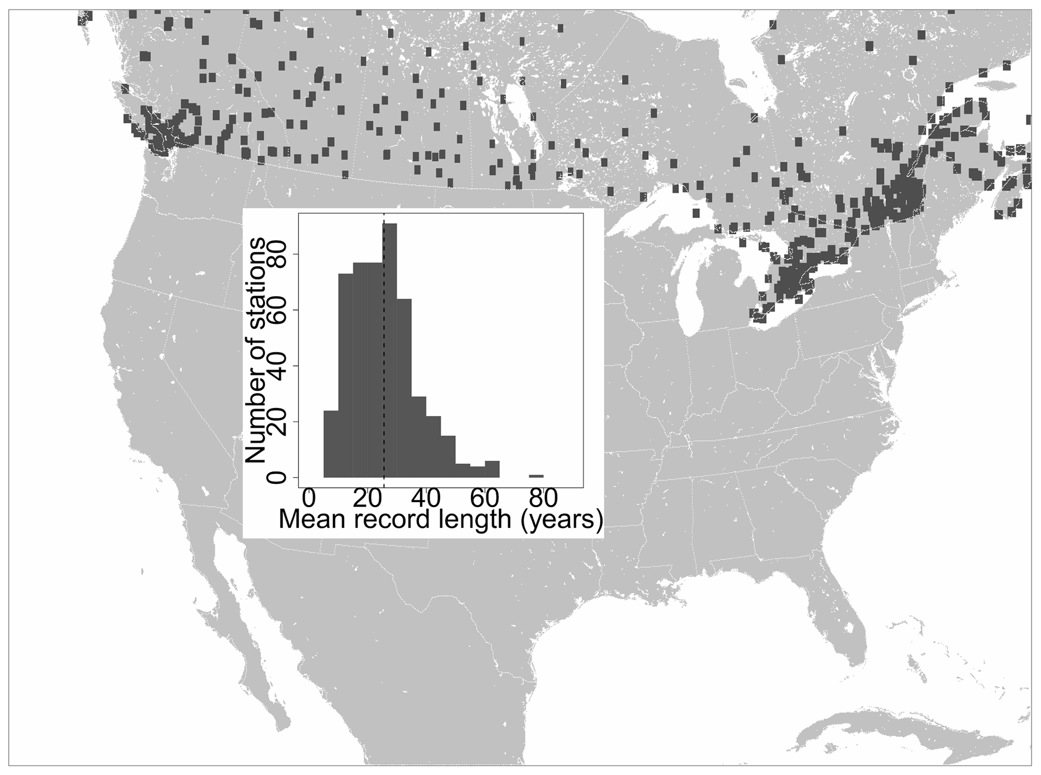
Figure 1 Map showing the NCAR HRCONUS WRF land mask and locations (rectangles) of the 488 IDF curve TBRG stations in Canada. The inset plot shows a histogram of mean record length (all IDF curve durations) at the stations; the median (vertical dashed line) is 25 years.

Precipitation outputs from the WRF CTRL simulations over the US have been evaluated against observations in several studies (e.g., Liu et al., 2017; Dai et al., 2017; Prein et al., 2017a, c; Raghavendra et al., 2018). To extend these results, the focus here is instead on the Canadian portion of the domain and the range of sub-daily to daily extremes communicated in IDF curves. Annual precipitation maxima at short durations are driven by rainfall, and hence the evaluation deals exclusively with extremes generated by rainstorms. In Canada, national IDF curves are disseminated by Environment and Climate Change Canada (ECCC, 2014) at more than 500 locations with long tipping-bucket rain gauge (TBRG) records; 488 stations fall within the WRF HRCONUS domain (Fig. 1) and are used in this study. TBRG record lengths range from 10 to 81 years, with a mean length of 25 years. Information on the observing program, quality control, and quality assurance methods is provided in detail by Shephard et al. (2014). IDF curves are derived from annual maximum rainfall extremes for accumulation durations ranging from 5 min to 24 h; model evaluation in this study will also focus on these data. For the WRF CTRL and PGW simulations, annual maximum rainfall intensities are calculated at land grid points for accumulation durations from 1 to 24 h. The first partial calendar year of the CTRL and PGW simulations is treated as spin-up and is not used in any calculations.

As a complement to the in situ observations, data from two observationally constrained gridded precipitation products are also considered. CMORPH CRT V1.0 is a near-global, reprocessed, and bias-corrected satellite precipitation product with 30 min temporal and ∼8 km spatial resolution (1998–2015) (Xie et al., 2017). Over land, CMORPH CRT adjusts raw CMORPH satellite precipitation estimates towards gauge analyses using a probability density function matching algorithm. MSWEP V2 is a global merged product that combines information from satellite, reanalysis, and gauge precipitation estimates at a 3 h temporal and 0.1^∘ spatial resolution (1979–2016) (Beck et al., 2017a, b). For consistency with the WRF CTRL simulations, annual maximum rainfall intensities are calculated for accumulation durations ranging from 1 to 24 h for CMORPH and from 3 to 24 h for MSWEP.

3 IDF curves and the GEVSS distribution

IDF curves provided by ECCC (2014) summarize the relationship between observed annual maximum rainfall intensity for specified frequencies of occurrence (2-, 5-, 10-, 25-, 50-, and 100-year return periods, i.e., 0.5, 0.8, 0.9, 0.96, 0.98, and 0.99 quantiles) and durations (5, 10, 15, 30, and 60 min and 2, 6, 12, and 24 h). Because TBRG records rarely exceed 50 years in length (Fig. 1), return value estimates at long return periods rely on statistical extrapolation guided by extreme value theory (Coles, 2001). In Canada, official IDF curves are constructed by first fitting the Gumbel distribution, i.e., the extreme value type I form of the GEV distribution, to annual maximum rainfall intensity series at each site for each duration (Hogg et al., 1989). At the majority of stations, the actual curves are then based on best-fit linear interpolation equations between log-transformed duration and log-transformed quantiles for each of the specified return periods. To illustrate, IDF curves for Victoria Intl. A., a station on the southwest coast of British Columbia, Canada, are shown in Fig. 2. Points indicate return values of rainfall intensity obtained from the fitted Gumbel distribution for each combination of return period and duration. IDF curves for each return period are based on log-log interpolating equations through these points and hence plotted as straight lines. While IDF curves produced in other national and subnational jurisdictions may be based on slightly different procedures and assumptions (Svensson and Jones, 2010), results are typically presented in a similar fashion and, broadly, share common characteristics.

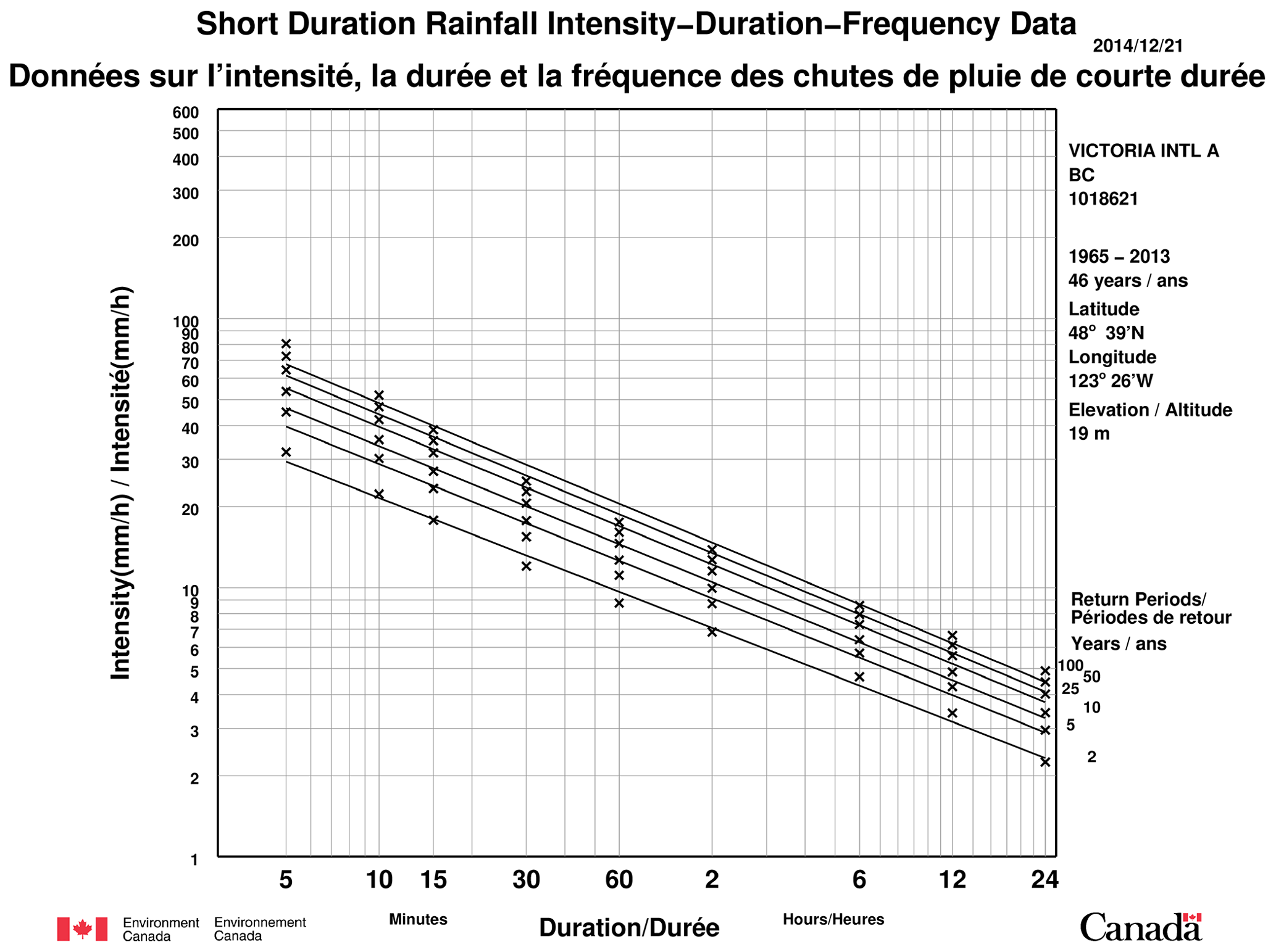
Figure 2 Example ECCC IDF data for Victoria Intl. A. (station 1018621) in British Columbia, Canada. Points (x) show quantiles associated with (from bottom to top) 2-, 5-, 10-, 25-, 50-, and 100-year-return-period intensities estimated by fitting the Gumbel form of the GEV distribution by the method of moments to annual maximum rainfall rate data for 5, 10, 15, 30, and 60 min and 2, 6, 12, and 24 h durations (left to right). Lines are from best-fit linear interpolation equations between log-transformed duration and log-transformed Gumbel quantiles for each return period.

For simplicity, the study starts with the ECCC IDF curve methodology as its basis. However, modifications to the standard approach are made to accommodate (1) the relatively short 13-year record lengths provided by the WRF CTRL and PGW simulations, (2) the underlying goal of assessing changes in general IDF curve characteristics (i.e., shifts and/or changes in IDF curve slope), and (3) the current state of the art of the analysis of rainfall extremes. More specifically, the two-step Gumbel–log-log interpolating equation approach is replaced with single-step estimation of IDF curves using a GEV simple scaling (GEVSS) distribution. Observational evidence suggests that daily rainfall extremes follow an extreme value distribution with a heavy upper tail (Papalexiou and Koutsoyiannis, 2013). Hence, a three-parameter GEV distribution, which includes the heavy-tailed type II extreme value or Fréchet form of the GEV distribution, is used rather than artificially restricting the GEV shape parameter to be zero (i.e., by using the two-parameter extreme value type I or Gumbel distribution). Separate GEV distribution parameters for each duration of interest, combined with separate interpolating equations for each quantile, leads to a very large number of statistical parameters that need to be estimated from relatively short WRF simulations. Despite the large forced signal and PGW experimental design, the limited sample size necessitates making efficient use of the available data. Hence, to reduce the overall number of distributional and regression parameters that need to be estimated, an aggregated GEVSS distribution is instead fitted to pooled annual maxima for all durations. The GEVSS model is based on the application of the simple scaling hypothesis – an empirical power-law relation that links the distributions of rainfall intensities at different durations – to the GEV distribution.

Use of the GEV distribution is motivated by the extreme value theorem, which states that the GEV is the only possible limit distribution for the maxima of a sequence of independent and identically distributed random variables (Coles, 2001). Defining $I_{D_{\mathrm{0}}}$ as the random variable of annual maximum rainfall intensity (mm h⁻¹) for an arbitrary reference duration, in this case D₀=24 h, it is assumed that samples of annual maxima are distributed according to the GEV distribution

$$\begin{array}{}\text{(1)}& \mathrm{Pr}(I_{D_{\mathrm{0}}}\le x)=\left\{\begin{array}{ll}\exp \left\{-{\left(\mathrm{1}+{\mathit{\xi }}_{\mathrm{0}}{\displaystyle \frac{x-{\mathit{\mu }}_{\mathrm{0}}}{{\mathit{\sigma }}_{\mathrm{0}}}}\right)}^{-\mathrm{1}/{\mathit{\xi }}_{\mathrm{0}}}\right\}& \mathrm{if}{\mathit{\xi }}_{\mathrm{0}}\ne \mathrm{0}\\ \exp \left\{-\exp \left(-{\displaystyle \frac{x-{\mathit{\mu }}_{\mathrm{0}}}{{\mathit{\sigma }}_{\mathrm{0}}}}\right)\right\}& \mathrm{if}{\mathit{\xi }}_{\mathrm{0}}=\mathrm{0}\end{array}\right.,\end{array}$$

where μ₀, σ₀>0, and ξ₀ are, respectively, the GEV location, scale, and shape parameters; ξ₀=0 corresponds to the type I extreme value distribution (Gumbel form), ξ₀>0 to the type II (Fréchet form), and ξ₀<0 to the type III (Weibull form). Quantiles associated with the T-year return period $T=\mathrm{1}/\left[\mathrm{1}-\mathrm{Pr}(I_{D_{\mathrm{0}}}\le x)\right]$ are determined by inverting the GEV cumulative distribution function given by Eq. (1).

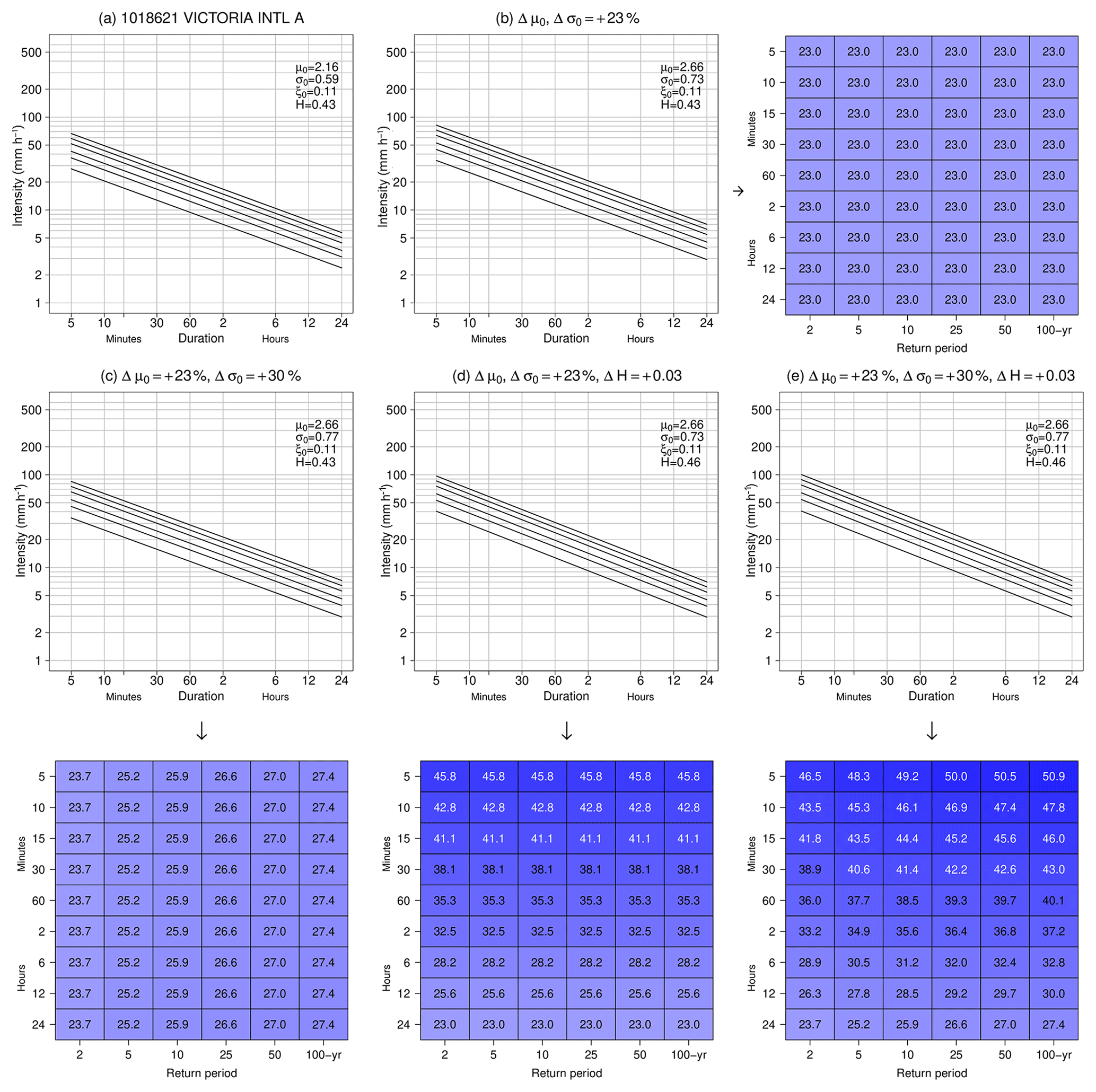
Figure 3 (a) Observed GEVSS IDF curves at Victoria Intl. A. (1018621) (see Fig. 2). Hypothetical IDF curves resulting from (b) increases of $\mathrm{\Delta }{\mathit{\mu }}_{\mathrm{0}}=+\mathrm{23}$ % and $\mathrm{\Delta }{\mathit{\sigma }}_{\mathrm{0}}=+\mathrm{23}$ % (i.e., no change in dispersion σ₀∕μ₀); (c) increases of $\mathrm{\Delta }{\mathit{\mu }}_{\mathrm{0}}=+\mathrm{23}$ % and $\mathrm{\Delta }{\mathit{\sigma }}_{\mathrm{0}}=+\mathrm{30}$ % (i.e., an increase in dispersion σ₀∕μ₀); (d) increases of $\mathrm{\Delta }{\mathit{\mu }}_{\mathrm{0}}=+\mathrm{23}$ %, $\mathrm{\Delta }{\mathit{\sigma }}_{\mathrm{0}}=+\mathrm{23}$ %, and $\mathrm{\Delta }H=+\mathrm{0.03}$; and (d) increases of $\mathrm{\Delta }{\mathit{\mu }}_{\mathrm{0}}=+\mathrm{23}$ %, $\mathrm{\Delta }{\mathit{\sigma }}_{\mathrm{0}}=+\mathrm{30}$ %, and $\mathrm{\Delta }H=+\mathrm{0.03}$. The matrix plots that accompany (b–d) show the associated percentage changes in return levels for each duration: (b) with constant H, increasing μ₀ and σ₀ without changing the dispersion leads to relative increases in return levels for all durations that match the relative changes in the underlying parameters; (c) increasing dispersion leads to return period dependence of changes, with larger relative increases evident at longer return periods; (d) increasing H steepens the IDF curves, which leads to duration dependence of changes; and (e) increases in both H and dispersion result in greater intensification at longer return periods and shorter durations. Note that values in (e) are based on domain mean values from Sect. 6.

To incorporate other durations, simple scaling makes the assumption that

$$\begin{array}{}\text{(2)}& I_D\stackrel{\mathrm{dist}}{=}{\left({\displaystyle \frac{D}{D_{\mathrm{0}}}}\right)}^{-H}{I}_{D_{\mathrm{0}}},\end{array}$$

where $\mathrm{0}<H<\mathrm{1}$ is a scaling exponent and $\stackrel{\mathrm{dist}}{=}$ means equality of distributions (Gupta and Waymire, 1990); for the GEV distribution (Nguyen et al., 1998), simple scaling implies that

$$\begin{array}{}\text{(3)}& {\mathit{\mu }}_D={\left({\displaystyle \frac{D}{D_{\mathrm{0}}}}\right)}^{-H}{\mathit{\mu }}_{\mathrm{0}};{\mathit{\sigma }}_D={\left({\displaystyle \frac{D}{D_{\mathrm{0}}}}\right)}^{-H}{\mathit{\sigma }}_{\mathrm{0}};{\mathit{\xi }}_D={\mathit{\xi }}_{\mathrm{0}}=\mathit{\xi }.\end{array}$$

The resulting GEVSS distribution for annual maximum rainfall intensities at different durations can be described by four parameters: location μ₀ and scale σ₀ parameters associated with the reference duration, a temporal scaling exponent H used to scale the reference location and scale parameters to other durations, and a shared shape parameter ξ for all durations. This leads to a simple expression for IDF curves at any duration and return period

$$\begin{array}{}\text{(4)}& i_{D,T}={\left({\displaystyle \frac{D}{D_{\mathrm{0}}}}\right)}^{-H}\left\{{\mathit{\mu }}_{\mathrm{0}}-{\displaystyle \frac{{\mathit{\sigma }}_{\mathrm{0}}}{\mathit{\xi }}}\left[\mathrm{1}-{\left(-\log \left[\mathrm{1}-{\displaystyle \frac{\mathrm{1}}{T}}\right]\right)}^{-\mathit{\xi }}\right]\right\},\end{array}$$

where i_D, T is the return level estimate for duration D and the T-year return period (Mélèse et al., 2018). In addition, changes in each parameter can be linked to changes in specific characteristics of IDF curves. For reference, hypothetical examples, based on the data shown in Fig. 2, are provided in Fig. 3. The scaling exponent H controls the common slope, in log-log space, of linear IDF curves for each quantile. Larger values lead to steeper IDF curves. Hence, increases in H provide direct evidence for stronger intensification of shorter-duration rainfall extremes than longer durations. The location μ₀ and scale σ₀ parameters control the vertical positioning (and hence changes lead to shifts) of the IDF curves. Furthermore, with constant ξ, changes in the non-dimensional dispersion coefficient σ₀∕μ₀ of the GEV distribution result in relative changes in return level that depend on return period; i.e., for a given duration, an increase in dispersion means that relative changes of more rare events will increase more than less rare events.

4 Parameter inference

Inferences about GEVSS parameters are made using a Bayesian framework (Van de Vyver, 2015; Mélèse et al., 2018). Posterior parameter distributions are obtained at each grid point from pooled 1, 3, 6, 12, and 24 h annual maximum rainfall intensities using the Metropolis–Hastings Markov chain Monte Carlo (MCMC) algorithm (Kruschke, 2015). The Bayesian GEVSS model for CTRL and PGW rainfall intensities is defined as

$$\begin{array}{ll}{\displaystyle }& {\displaystyle }{I}_{D_{\mathrm{CTRL}}}\sim \mathrm{GEVSS}\left({\mathit{\mu }}_{{\mathrm{0}}_{\mathrm{CTRL}}},{\mathit{\sigma }}_{{\mathrm{0}}_{\mathrm{CTRL}}},\mathit{\xi },H_{{}_{\mathrm{CTRL}}}\right)\\ {\displaystyle }& {\displaystyle }{I}_{{\mathrm{D}}_{\mathrm{PGW}}}\sim \mathrm{GEVSS}\left({\mathit{\mu }}_{{\mathrm{0}}_{\mathrm{PGW}}},{\mathit{\sigma }}_{{\mathrm{0}}_{\mathrm{PGW}}},\mathit{\xi },H_{\mathrm{PGW}}\right)\\ \text{(5)}& {\displaystyle }& {\displaystyle }{D}_{\mathrm{0}}=\text{24\hspace{0.17em}h},D=\mathit{\left\{}\text{1,\hspace{0.17em}3,\hspace{0.17em}6,\hspace{0.17em}12,\hspace{0.17em}24\hspace{0.17em}h}\mathit{\right\}},{\displaystyle }& {\displaystyle }{\mathit{\mu }}_{{\mathrm{0}}_{\mathrm{CTRL},\mathrm{PGW}}}\sim U\left(\mathrm{0.01}{\stackrel{\mathrm{‾}}{i}}_{{\mathrm{0}}_{\mathrm{CTRL}}},\mathrm{4}{\stackrel{\mathrm{‾}}{i}}_{{\mathrm{0}}_{\mathrm{CTRL}}}\right)\\ {\displaystyle }& {\displaystyle }{\mathit{\sigma }}_{{\mathrm{0}}_{\mathrm{CTRL},\mathrm{PGW}}}\sim U\left(\mathrm{0.01}{\stackrel{\mathrm{‾}}{i}}_{{\mathrm{0}}_{\mathrm{CTRL}}},\mathrm{4}{\stackrel{\mathrm{‾}}{i}}_{{\mathrm{0}}_{\mathrm{CTRL}}}\right)\\ {\displaystyle }& {\displaystyle }\mathit{\xi }\sim N\left(\mathrm{0.114},\mathrm{0.045}\right)\\ \text{(6)}& {\displaystyle }& {\displaystyle }{H}_{{}_{\mathrm{CTRL},\mathrm{PGW}}}\sim U\left(\mathrm{0},\mathrm{1}\right),\end{array}$$

where GEVSS, U, and N refer to the GEVSS, normal, and uniform distributions with specified parameters, respectively, and ${\stackrel{\mathrm{‾}}{i}}_{{\mathrm{0}}_{\mathrm{CTRL}}}$ is the sample mean 24 h annual maximum rainfall intensity for the WRF CTRL simulation. A relatively broad uniform prior distribution, with limits constrained to be positive multiples of ${\stackrel{\mathrm{‾}}{i}}_{{\mathrm{0}}_{\mathrm{CTRL}}}$, is used for both the location μ₀ and scale σ₀ parameters of the CTRL and PGW simulations. This choice is informed by past work showing (1) that end-of-century projected changes in annual rainfall extremes by CMIP5 models, which scale similarly to μ₀ and σ₀, are expected to be less than half the upper limit of the prior (Kharin et al., 2013; Toreti et al., 2013; Cannon et al., 2015) and (2) that observational estimates of the dispersion σ₀∕μ₀ for daily rainfall extremes in North America are on the order of ∼0.2 (Koutsoyiannis, 2004). While this implies that a narrower prior could be used for σ₀, a more conservative choice is adopted here. Following Kharin et al. (2013) and related work, it is assumed that the shape parameter ξ is the same in the CTRL and PGW periods (see below for more details). The normal prior distribution used for ξ follows from an analysis of daily station observations by Papalexiou and Koutsoyiannis (2013), who found that ξ varies globally in a narrow range $\mathrm{0}<\mathit{\xi }<\mathrm{0.23}$. Finally, the uniform distribution between 0 and 1 for H follows from Van de Vyver (2015).

Posterior distributions for GEVSS parameters at each grid point are estimated from 100 000 MCMC samples taken following a burn-in period of 10 000 samples. Standard diagnostics (e.g., Geweke, Ratery–Lewis, and Heidelberg–Welch tests; Plummer et al., 2006) are used to assess convergence of the chain; these are complemented by spot visual inspections at randomly selected grid points. Because of the high model resolution, large domain, and associated storage cost, the MCMC chain is thinned to 1000 samples by saving every 100th sample. All subsequent results are based on the thinned chain. The independence likelihood is used for the GEVSS model. Hence, the model is, from a strict standpoint, misspecified as simulated annual rainfall extremes for different durations can be generated by the same storm system. Implications of this lack of independence on the posterior distributions are examined via Monte Carlo simulation in the Supplement (Fig. S1 in the Supplement). Results suggest that posterior distributions for μ₀ and σ₀ are slightly too narrow when the independence assumption is violated, but those for ξ and H are reliable. To test the stationarity assumption for ξ, separate models in which ξ was free to differ between the CTRL and PGW simulations are also considered. Modified deviance information criterion (DIC^*) differences between the nonstationary and stationary models (Spiegelhalter et al., 2014) and posterior distributions of the ξ_PGW−ξ_CTRL differences for the nonstationary model (Fig. S2) confirm that the assumption of constant shape is reasonable. Subsequent results are thus reported for the stationary ξ model; unless noted otherwise, results are based on posterior means.

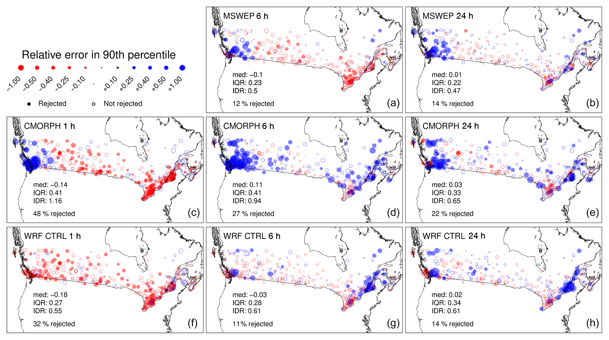
Figure 4 Relative error (RE) in the empirical 90th percentile (10-year return level) of annual maximum rainfall intensities between each MSWEP (a, b), CMORPH (c, d, e), and WRF CTRL (f, g, h) gridded dataset and station observation for 1 h (c, f), 6 h (a, d, g), and 24 h (b, e, h) accumulation durations. Summary statistics reported in each figure include the median (med), interquartile range (IQR), and interdecile range (IDR) of RE, as well as the percentage of locations exhibiting statistically significant values of RE. Statistical testing is performed at the 0.05 significance level.

5 Historical model evaluation

Prior to assessing projected changes in extreme rainfall and IDF curve characteristics, evaluations are first conducted to assess whether (1) extreme rainfall in the WRF CTRL simulation is well-simulated; (2) whether the GEVSS statistical model assumptions are met; and, finally, whether (3) WRF CTRL IDF curve estimates based on the GEVSS statistical model are consistent with those from observations. As noted above, simulated rainfall extremes from the WRF CTRL simulation have already been evaluated against station data over the US (e.g., Figs. S2–S4 in Prein et al., 2017c, which led the authors to conclude that “the control simulation is able to reproduce the observed intensity and frequency of extreme hourly precipitation in most parts of CONUS”). The focus here is thus on the Canadian portion of the domain.

Annual maxima from in situ observations arguably represent the most accurate and reliable estimates of extreme rainfall, despite instrumental uncertainty and limited spatiotemporal coverage. For this reason, extremes from the WRF CTRL simulation are first assessed against 488 IDF curves derived from data at TBRG stations; the station locations are shown in Fig. 1. Because extreme rainfall is a non-negative quantity with substantial spatial variation over the domain, model performance statistics used for evaluation are based on the accuracy ratio ${\mathrm{AR}}_i=\widehat{y_i}/y_i$ or, equivalently, relative error (or bias) ${\mathrm{RE}}_i={\mathrm{AR}}_i-\mathrm{1}$, where y_i and $\widehat{y_i}$ are observed and modelled values for i=1 … N locations. Grid points in each dataset are matched with the nearest neighbouring station. Statistics include the mean logarithmic accuracy ratio (MLAR), which summarizes relative bias,

$$\begin{array}{}\text{(7)}& \mathrm{MLAR}={\displaystyle \frac{\mathrm{1}}{N}}\sum _{i=\mathrm{1}}^N{\log }_{\mathrm{10}}\left({\mathrm{AR}}_i\right),\end{array}$$

and mean absolute logarithmic accuracy ratio (MALAR), which summarizes overall magnitude of relative error,

$$\begin{array}{}\text{(8)}& \mathrm{MALAR}={\displaystyle \frac{\mathrm{1}}{N}}\sum _i\left|{\log }_{\mathrm{10}}\left({\mathrm{AR}}_i\right)\right|.\end{array}$$

Notably, LAR-based statistics, unlike those based on untransformed RE, are symmetric measures of relative error, i.e., proportional errors of 1∕10 and 10 are assigned equal magnitudes (−1 and +1, respectively).

For comparison, results are also provided for the CMORPH and MSWEP observationally constrained gridded datasets (Table 1), bearing in mind that both products are directly informed by station observations within the WRF domain and are thus not strictly independent from the verification data. Also, it is assumed that the 4 km WRF, 0.073^∘ CMORPH, and 0.1^∘ MSWEP grids are of sufficiently high resolution that they can be meaningfully compared against in situ data, notwithstanding differences in interpolation and gridding methods, grid area (nominally 16 to ∼85 km² at the median station latitude), and inherent issues with area-to-point comparisons. To investigate the latter issue, MLAR and MALAR performance statistics are also calculated after rescaling quantiles from the gridded datasets based on empirical areal reduction factors (ARFs) from Kjeldsen (2007); these corrected values are reported in Figs. S3–S5. Values in the main text are based on raw, uncorrected quantile estimates.

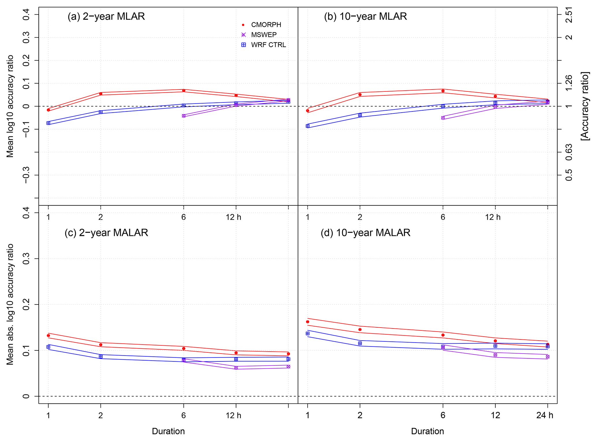
Figure 5 Summaries of MLAR and MALAR for the empirical 50th (2-year return level) and 90th percentile (10-year return level) of annual maximum rainfall intensities between each MSWEP, CMORPH, and WRF CTRL gridded dataset and station observation for 1 to 24 h accumulation durations. Solid lines indicate the 95 % confidence interval. Perfect performance is indicated by the horizontal dashed lines.

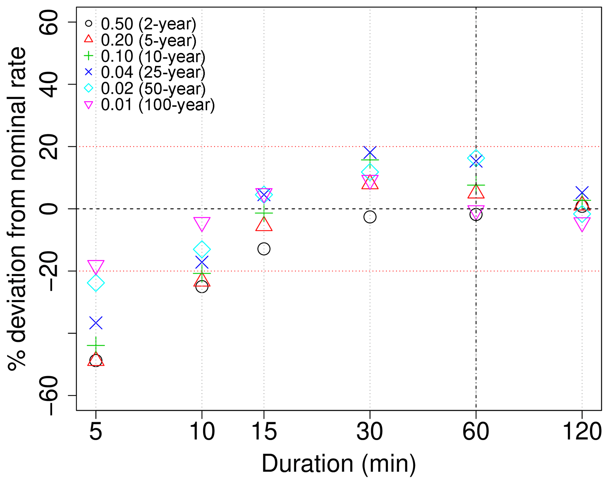
Figure 6 Posterior predictive checks for sub-hourly durations extrapolated from GEVSS distributions fitted to observed annual maxima for durations ≥60 min. Values are relative deviations from nominal exceedance rates for 2- to 100-year return level estimates (i.e., 50 % to 1 % chance of exceedance, respectively). Perfect reliability is indicated by the horizontal black dashed line; deviations of ±20 % are indicated by horizontal red dotted lines.

Before summarizing performance in terms of MLAR and MALAR, maps of RE for the empirical 90th percentile (10-year return level) of annual maximum rainfall between the gridded datasets and station observations are shown in Fig. 4 for 1, 6, and 24 h durations. A permutation test is used to estimate the statistical significance of the RE values. The permutation test considers a null hypothesis of equal quantiles between station and grid box distributions. Under this null hypothesis, station and grid box annual maxima at a given location are combined into a single sample. The combined data are then randomly reassigned to two permutation resamples (i.e., two series of shuffled annual maxima) having equal length as the original un-permuted station and grid box samples. For each station–grid box pair, the distribution of the RE statistics is approximated using 5000 random permutation resamples and the p value is computed as the fraction of resamples generating RE absolute values equal to or larger than those observed on the original annual maxima samples.

Due to the short WRF record length, empirical return levels for return periods longer than 10 years are not considered. For all stations and grid points, empirical quantiles are calculated based on the entire period of record, which differs in length at each station and product. While this will result in some level of unknown station-dependent bias, there is limited evidence to suggest that historical trends in annual maximum short-duration rainfall intensity are detectable at individual stations (Shephard et al., 2014; Barbero et al., 2017); an argument can thus be made in favour of using as much data as possible for estimation, rather than harmonizing the periods of record.

Figure 4 indicates that performance of WRF in terms of RE reaches or, in some cases, exceeds that of the best observationally constrained product. Spatially, RE for WRF and the two gridded observational products is generally low over the interior of the domain for 6 and 24 h durations. Bias is largest over coastal regions and the western Cordillera, where both the simulations and gridded observations tend to overestimate the 10-year return level. Notably, MSWEP and WRF perform better than CMORPH at these two durations. For the 24 h (6 h) duration, significant RE values are found at 14 % (12 %) of stations for MSWEP, 14 % (11 %) for WRF, and 22 % (27 %) for CMORPH. Performance at the shortest 1 h duration degrades for both CMORPH and WRF – the two gridded products with a sampling frequency <3 h – with significant RE found at 48 % and 32 % of stations, respectively. In both cases, 10-year return levels tend to be underestimated, except in the west for CMORPH, with median RE values of −0.14 and −0.18 for CMORPH and WRF, respectively. Note, however, that results are more consistent for WRF (interquartile and interdecile ranges of 0.27 and 0.55 versus 0.41 and 1.16 for CMORPH).

MLAR and MALAR, which provide aggregated measures of performance over the in situ station network, are shown in Fig. 5 for quantiles associated with the 2- and 10-year return levels for each of the 1, 2, 6, and 24 h durations. Values are accompanied by 95 % confidence intervals estimated based on 1000 bootstrap samples drawn from the series of annual maxima at each location. The pattern of relative bias across durations for WRF and the two sets of gridded observations, expressed in terms of MLAR, is similar for the 2- and 10-year return levels. All datasets show similar values of MLAR at the 24 h duration, whereas WRF outperforms CMORPH for durations from 2 to 12 h, and MSWEP at the 6 h duration. WRF underestimates more than CMORPH at the shortest 1 h duration, but the overall level of bias is still modest for both datasets. However, when contributions from both systematic and unsystematic errors are taken into consideration via MALAR, WRF is found to outperform CMORPH for both return levels and all durations. MSWEP performs best for the 12 and 24 h durations but is matched by WRF at the 6 h duration.

When empirical quantiles of the gridded data are adjusted to account for area-to-point comparisons, i.e., by rescaling by inverse ARFs from Kjeldsen (2007), performance of WRF relative to CMORPH improves, especially at the shortest durations (Fig. S3). While WRF performs better at 1 and 2 h durations following adjustment, the performance of CMORPH degrades at all durations, which suggests that it may be overpredicting extreme rainfall at its nominal native resolution. Significant improvements in performance of MSWEP are also noted at the 6 h duration. Results must, however, be treated with caution, given that ARFs are empirical and are an imperfect, approximate way to harmonize area and point extremes.

In addition to verifying that WRF can reliably simulate sub-daily rainfall extremes, the ability of the GEVSS statistical model to describe the distribution of annual rainfall maxima must also be checked. One of the advantages of the GEVSS model is that it can be used to extrapolate from available durations to shorter durations, e.g., from simulated 1 h data to sub-hourly durations needed in IDF curves or building codes. However, the ability to extrapolate depends strongly on the GEVSS goodness of fit, especially for the shortest durations for which the simple scaling hypothesis may no longer hold (Innocenti et al., 2017). If the GEVSS model is consistent with observations, then observed exceedance probabilities of the predicted quantiles should match nominal values. For example, 10 % of station observations should exceed the predicted 10-year return levels (the 90th percentiles), and so forth. Results from posterior predictive checks of the GEVSS distribution for observed annual maxima are shown in Fig. 6. In this case, the GEVSS distribution is fitted to pooled 1, 2, 6, 12, and 24 h duration observations at each station, and predictive quantiles are computed and compared against observations for sub-hourly data not used to fit the model. As expected, results are consistent with observations for the 1 and 2 h durations used to fit the GEVSS model. The model continues to perform reliably when extrapolating to the 30 and 15 min durations but begins to deviate from the nominal exceedance probabilities for the 10 min duration. Expected exceedance probabilities are underestimated by ∼20 %–55 % at the 5 min duration, suggesting that predicted GEVSS return levels are overpredicted; results for the shortest durations should thus either not be used or be treated with caution.

Given findings above that (1) daily and sub-daily rainfall extremes from the WRF model are generally well-simulated and (2) that the GEVSS distribution provides an acceptable fit to station observations for durations >10 min, GEVSS IDF curves derived from WRF outputs should resemble those calculated directly from in situ observations. To verify that this is indeed the case, IDF curve return levels estimated from WRF (and, for reference, CMORPH and MSWEP) are compared with those calculated from station observations. (A separate intercomparison is presented for GEVSS parameters in Figs. S6–S8.) The observational reference in this case is the set of return level estimates from IDF curves disseminated by ECCC (i.e., calculated using the two-step Gumbel–log-log regression methodology outlined in Sect. 3). Furthermore, uncertainty due to differences in estimation methodology is examined by comparing the ECCC IDF curves with those obtained by fitting the GEVSS distribution to station data. This is carried out for GEVSS-based estimates from the full set of observed durations (5 min to 24 h) and a restricted set of durations (1 to 24 h) to match the sampling frequency of the WRF outputs. Results are shown for relative bias (MLAR) in Fig. 7 and for relative error magnitude (MALAR) in Fig. 8. In all cases, posterior means and 95 % credible intervals for the MLAR and MALAR statistics are estimated from the posterior distributions of the GEVSS parameters and the resulting return levels.

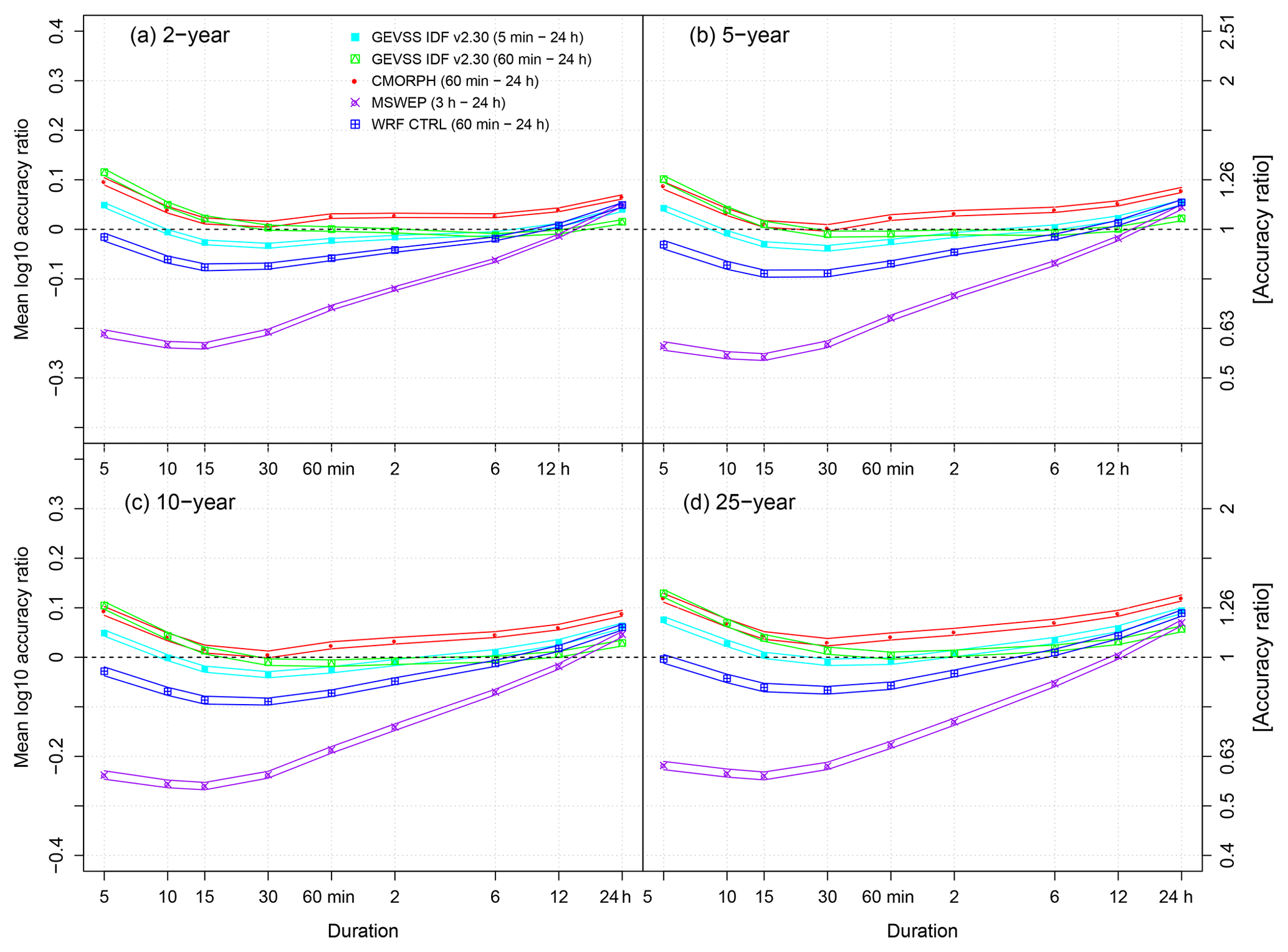
Figure 7 Summaries of MLAR for the GEVSS (a) 50th (2-year return level), (b) 80th (5-year return level), (c) 90th (10-year return level), and 96th (25-year return level) percentile estimates of annual maximum rainfall intensities for each MSWEP, CMORPH, and WRF CTRL gridded dataset. Results are compared with ECCC IDF curve v2.30 estimates for 5 min to 24 h accumulation durations at 488 TBRG stations. For reference, values are shown for GEVSS IDF curve estimates based on 5 min to 24 h TBRG data and a restricted set of 60 min to 24 h durations. Solid lines indicate the 95 % credible interval. Perfect performance is indicated by the horizontal dashed lines.

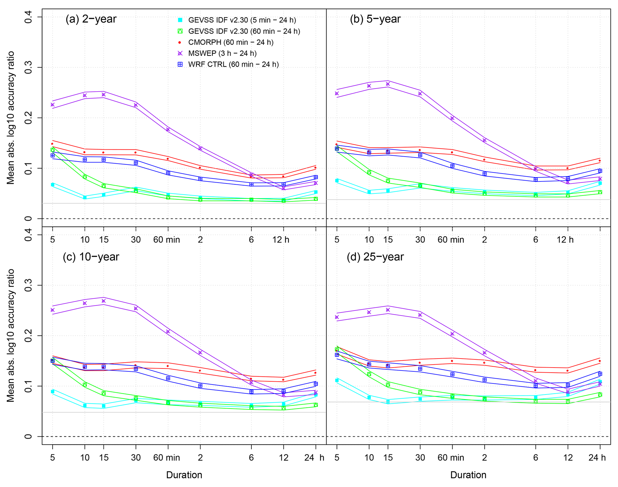
Figure 8 As in Fig. 7, but for MALAR. For reference, the horizontal gray line indicates the expected MALAR for empirical quantile estimates, based on 25-year samples (the median record length of TBRG station observations), from a true $\mathrm{GEV}(\mathit{\mu }=\mathrm{1.93},\mathit{\sigma }=\mathrm{0.64},\mathit{\xi }=\mathrm{0.10})$ distribution; parameters correspond to median estimates at the 488 IDF curve TBRG stations.

Fitting the GEVSS distribution to station data results in IDF curves that are largely similar to the official ECCC IDF curves. When fitting to all observed durations, differences are small, even for sub-hourly durations. When the set of fitted durations is restricted to be ≥1 h and the GEVSS distribution is used to extrapolate to sub-hourly durations, estimates are consistent with the ECCC IDF curves down to the 15 min duration; overprediction is evident at the shortest 5 and 10 min durations. Turning now to GEVSS IDF curves estimated from WRF CTRL outputs, results indicate that WRF is generally equally consistent or more consistent than CMORPH with ECCC IDF curves for all durations and return levels. The same is true when WRF is compared with MSWEP for durations ≤6 h.

Values of MLAR and MALAR calculated following ARF adjustment of gridded data are shown in Figs. S4 and S5, respectively. For WRF, area-to-point correction improves the level of consistency with GEVSS estimates based on in situ station data. In particular, no statistically significant differences in MLAR are found for 5 min to 6 h IDF curves between WRF- and GEVSS-based estimates from the restricted set of durations; minimal bias is found for durations from 15 min to 6 h. This is accompanied by reductions in MALAR and, hence, overall relative error. For CMORPH and MSWEP, area-to-point correction leads to opposite changes in performance. Relative bias and error become worse for CMORPH, whereas performance of MSWEP is improved substantially for durations less than 12 h.

6 Future projections

The main goal of this study is to investigate how IDF curve characteristics are projected to change in convection-permitting climate model simulations. From a statistical perspective, this is achieved by making inferences about changes in the parameters of the GEVSS distribution. Inference is based on posterior distributions of differences in parameters between the CTRL and PGW simulation periods.

For example, if the goal is to assess whether there is evidence for a steepening of IDF curves in the future,

$$\begin{array}{}\text{(9)}& \mathrm{\Delta }{H}_{\mathrm{PGW}-\mathrm{CTRL}}>\mathrm{0},\end{array}$$

then values of the posterior error probability (PEP), defined as $\mathrm{Pr}(\mathrm{\Delta }{H}_{\mathrm{PGW}-\mathrm{CTRL}}\le \mathrm{0})$, are determined from the posterior parameter distributions at each grid point. To account for the problem of multiple comparisons, the PEP values are evaluated under a Bayesian FDR framework – a Bayesian analogue of the approach recommended by Wilks (2016) – using a global FDR of 10 % following Storey et al. (2003), Käll et al. (2008), and as summarized by Robinson (2017). Based on the PEP, grid points with sufficient evidence for an increase are identified such that no more than 10 % are included by mistake, i.e., the probability of correctly identifying an increase in a given parameter at a grid point is at least 90 %. Conversely, one can evaluate evidence for decreases in GEVSS parameters by reversing the definition of PEP.

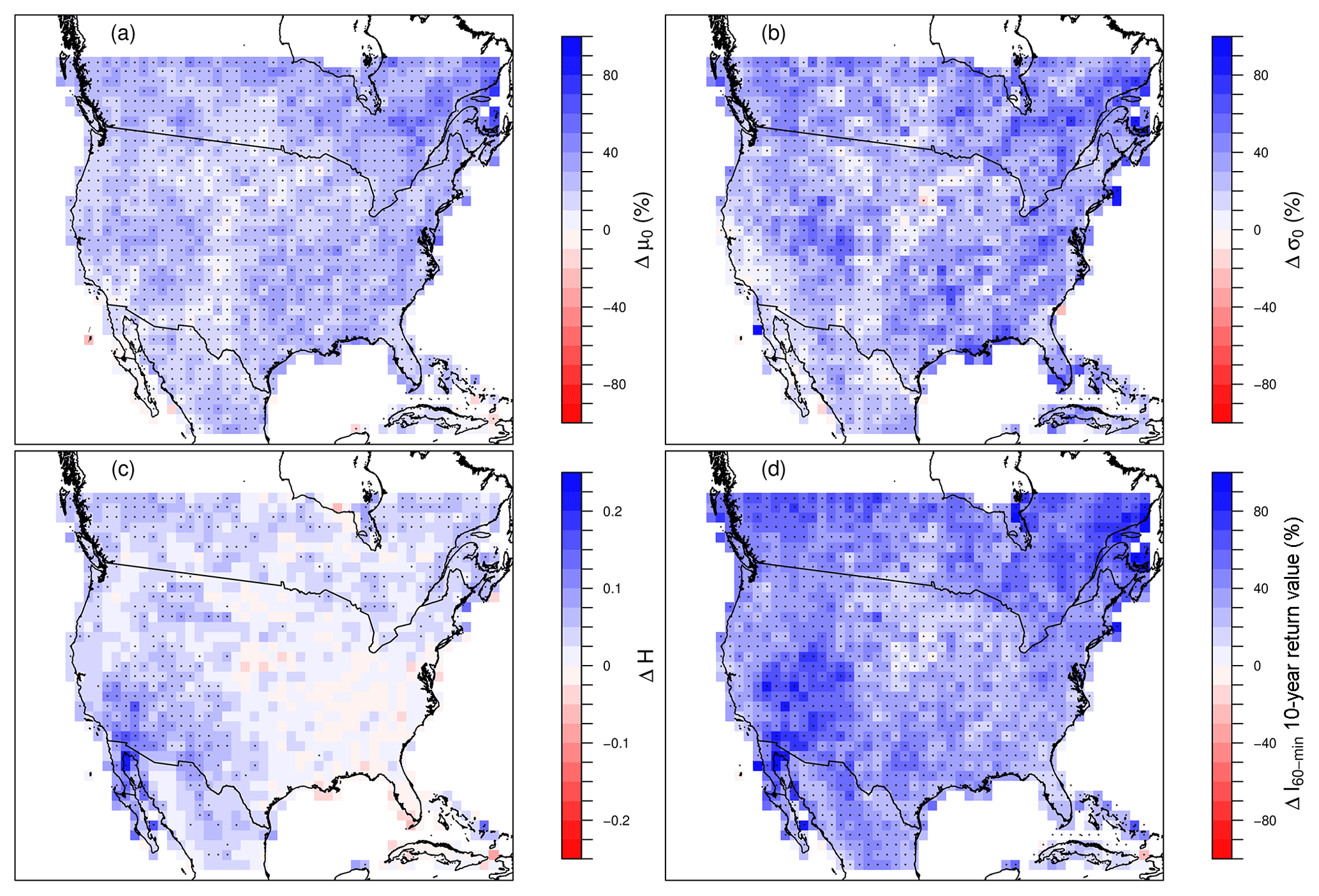
Figure 9 Projected changes in GEVSS (a) location μ₀, (b) scale σ₀, and (c) scaling exponent H parameters, as well as changes in (d) 10-year return level 1 h duration rainfall extremes I_{60 min, 10 years}. For ease of visualization, results are aggregated to a 100 km × 100 km grid. Values shown are aggregated grid box means; boxes in which more than half of the 4 km WRF grids show significant increases (decreases) are marked with a * (∕).

Projected PGW–CTRL changes over the domain are shown in Fig. 9. Significant increases in GEVSS location (>99 % of grid points), scale (>88 %), and scaling exponent (>39 %) parameters are projected over large portions of the domain, whereas almost no significant decreases in the GEVSS parameters are projected to occur (<1 %, <5 %, and <5 % respectively). The result is that IDF curves tend to shift upward and, with the exception of the eastern US, steepen, which leads to the largest increases in return values for short-duration extremes at the end of the 21st century. For example, at the 1 h duration, the median projected increase in the 10-year return value (Fig. 9d) is +38 % (+29 % lower quartile, +49 % upper quartile), versus +25 % (+18 %, +33 %) for the 10-year return level of the 24 h duration. The projected increase in the GEVSS scaling exponent calls into question stationarity assumptions (i.e., that daily to sub-daily scaling remains the same) that form the basis for existing IDF curve projections that rely exclusively on simulations at the daily timescale.

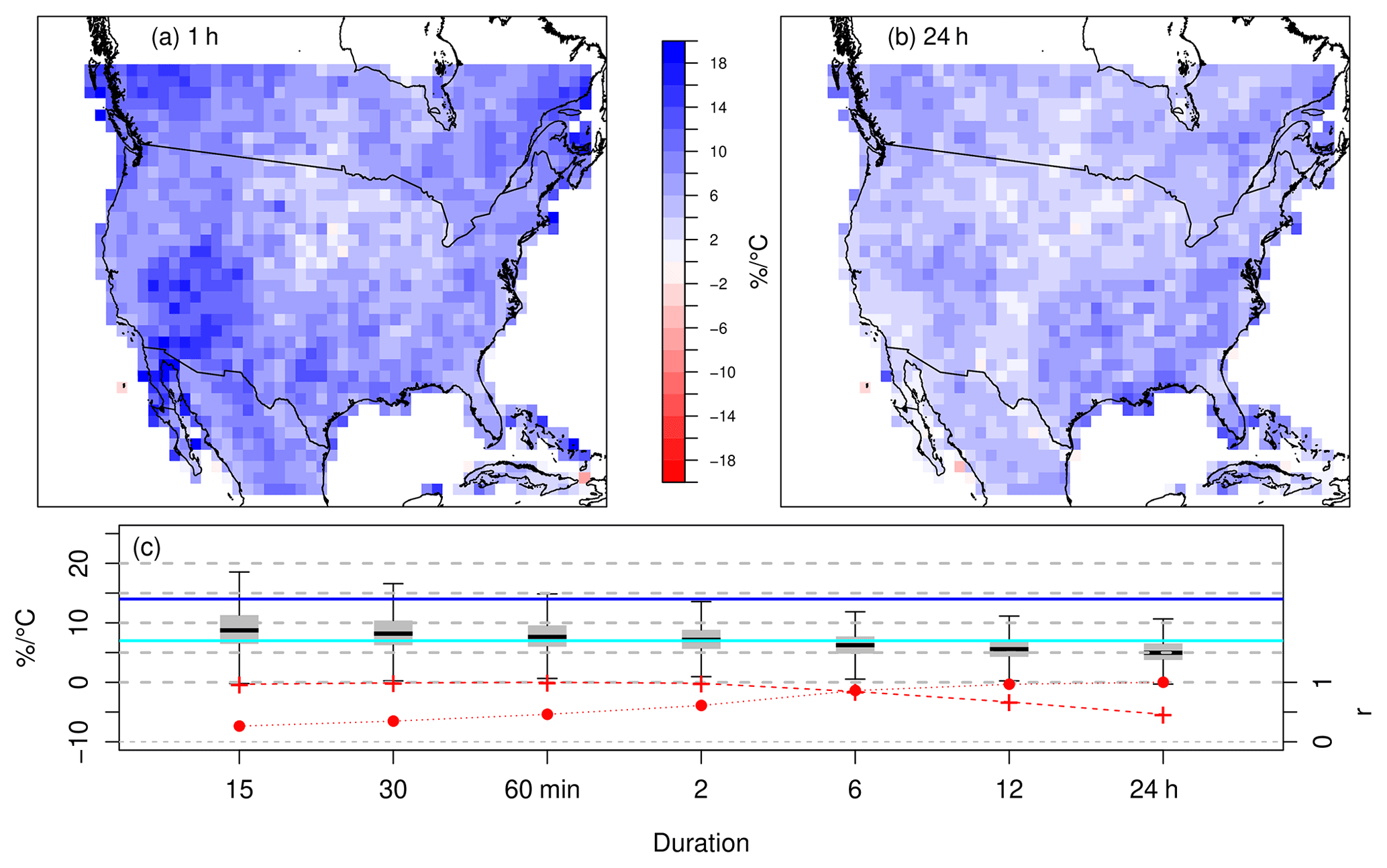
Figure 10 Temperature scaling of 10-year return levels of (a) 1 h and (b) 24 h extreme rainfall; values shown are aggregated 100 km × 100 km grid box means. (c) Box plots summarizing the distribution of temperature scaling values for 10-year return levels of 15 min to 24 h duration extreme rainfall. The horizontal line in the middle of each box indicates the median, boxes extend from the lower quartile to the upper quartile, and the whiskers extend to 1.5 times the IQR. The horizontal cyan (blue) line indicates temperature scaling of 7 % ^∘C⁻¹ (14 % ^∘C⁻¹). The red dashed (dotted) lines and the secondary vertical axis indicate the spatial correlation between maps of temperature scaling for each duration and the 1 h (24 h) maps.

These findings are for a strong +3.5 ^∘C global warming signal that corresponds to end-of-century conditions under the RCP8.5 scenario, which limits their general usefulness. Given that there is little evidence to suggest that changes in precipitation extremes for a given temperature change depend on RCP forcing scenario over North America (Pendergrass et al., 2015), results are reframed in terms of local scaling with annual mean temperature change. Assuming that the temperature scaling relationship holds, which may depend on the relative composition of aerosol vs. greenhouse gas forcings (Lin et al., 2016), future projections of local temperature can then be used to gain information about future return levels of extreme rainfall. Temperature scaling results for the 1 and 24 h 10-year return levels are shown in Fig. 10a and b, respectively, with summaries for the other durations shown in Fig. 10c. Based on the model evaluation presented in Sect. 5, results are not shown for the 5 and 10 min durations. Median temperature scaling values for 1 h (7.6 % ^∘C⁻¹) to 6 h (6.2 % ^∘C⁻¹) durations are consistent with the CC relation (∼6 % ^∘C⁻¹ to 8 % ^∘C⁻¹ over the range of temperatures simulated by WRF), although with some regional variation. Notably, larger scaling magnitudes are found over coastal regions and a region extending northward from the Baja California Peninsula into the Great Basin. Scaling rates in the interior of the continent – the Great Plains and Central Lowland – tend to be smaller. Sub-hourly durations share the same spatial pattern, but with overall enhancement of temperature scaling (median values of 8.7 % ^∘C⁻¹ at 15 min and 8.2 % ^∘C⁻¹ at 30 min). Given the form of the GEVSS model, however, note that results at sub-daily durations are strongly influenced by projected changes in the scaling exponent parameter H (see Fig. 9c). At longer durations, median scaling rates are lower (5.6 % ^∘C⁻¹ at 12 h and 5.0 % ^∘C⁻¹ at 24 h) and are more spatially uniform, without as strong of a gradient between coastal and interior regions. For reference, temperature scaling of GEVSS parameters, rather than return levels, is provided in Fig. S9.

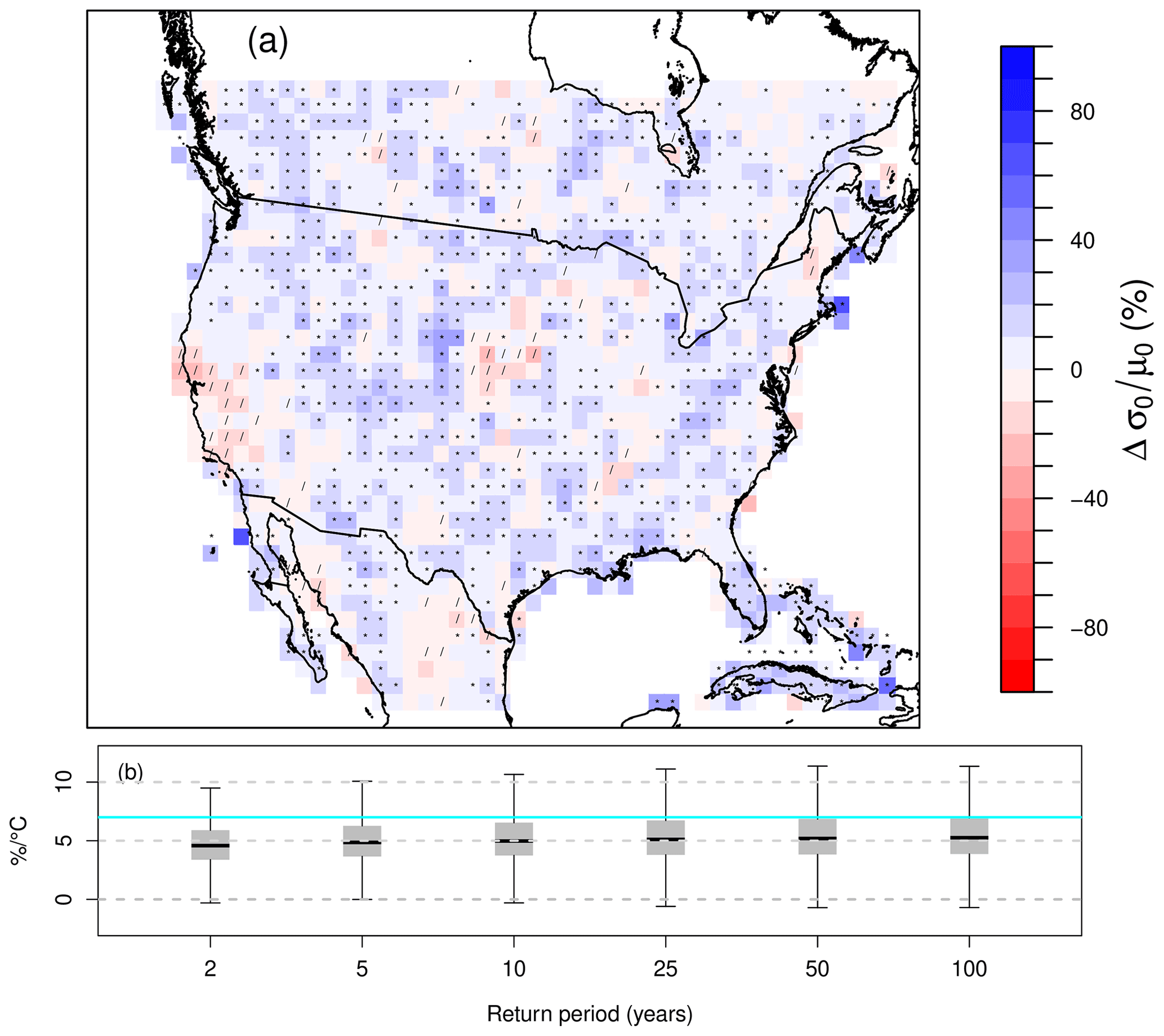
Figure 11 Projected changes in (a) GEVSS dispersion σ₀∕μ₀. Values shown are aggregated 100 km × 100 km grid box means; boxes in which more than half of the 4 km WRF grids show significant increases (decreases) are marked with a * (∕). (b) Box plots summarizing the distribution of temperature scaling values for 2- to 100-year return levels of 24 h duration extreme rainfall; the horizontal cyan line indicates temperature scaling of 7 % ^∘C⁻¹.

Given a constant shape ξ parameter between the CTRL and PGW simulations, relative changes in return levels from the GEVSS distribution can vary across return periods only if the dispersion σ₀∕μ₀ is projected to change. Over North America, Kharin et al. (2018) found that CMIP5 models with parameterized convection project greater intensification of more rare, more intense extreme daily precipitation events than less rare, less intense events. Results from the convection-permitting WRF simulations are shown in Fig. 11. Projected changes in σ₀∕μ₀ are predominantly positive; spatially coherent regions with significant increases are found over 50 % of the domain. This leads to a modest dependence of relative changes in return levels on return period. When expressed in terms of temperature scaling, median values for the 24 h duration – the reference duration in the GEVSS model – increase from 4.6 % ^∘C⁻¹ for the 2-year return period to 5.3 % ^∘C⁻¹ for the 100-year return period.

7 Discussion and conclusions

Annual maximum sub-daily and daily rainfall outputs from continental-scale decadal simulations of WRF are combined with a parsimonious GEVSS model, which “borrows strength” from multiple durations to improve parameter estimation, to assess changes in IDF curve characteristics over North America. The GEVSS model allows for non-zero shape parameter but constrains all quantile curves to share the same slope. This reduces the number of parameters relative to the official ECCC IDF curves, while keeping the main characteristics of the conventional approach, but also allowing some flexibility in terms of the ability to model heavy-tailed distributions. Comparisons of model performance statistics between GEVSS estimates and official ECCC IDF v2.30 values indicate that systematic and unsystematic errors are, in general, very low, which suggests that the two methodologies provide similar quantile estimates. In particular, for durations ≥15 min, the GEVSS model leads to IDF curve estimates that are consistent with official ECCC IDF curves at TBRG stations in Canada, mirroring findings of Innocenti et al. (2017). In agreement with previous climate model evaluations that have focused on the US (e.g., Prein et al., 2017c), WRF is found to provide credible simulations of historical annual maximum short-duration rainfall and associated IDF curves over the Canadian portion of the domain.

Projected changes in GEVSS parameters are evaluated using a Bayesian FDR framework. Large portions of the domain experience significant increases in GEVSS location μ₀ (>99 % of grid points), scale σ₀ (>88 %), and scaling exponent H (>39 %) parameters in the PGW simulation (+3.5 ^∘C global warming signal). Increases in each GEVSS parameter are linked to changes in specific characteristics of IDF curves. In particular, IDF curves tend to shift upward (increases in μ₀ and σ₀) and, with the exception of the eastern US, steepen (increases in H). This leads to the largest increases in return levels for short-duration extremes. In addition, spatially coherent but small increases in dispersion of the GEVSS distribution are found over more than half of the domain, providing some evidence for return period dependence of future changes in extreme rainfall. When changes in extremes are scaled according to projected regional temperature change, median scaling rates follow the CC relation at 1 to 6 h durations, which is consistent with CC scaling found by Prein et al. (2017c) for hourly extremes. Spatial patterns and dependence of the temperature scaling relationships on duration are also consistent with results found for station records in Canada (Panthou et al., 2014), although care must be taken due to differences in scaling definitions (e.g., Zhang et al., 2017). Modest sub-CC scaling at longer durations and modest super-CC scaling at sub-hourly durations are found for other timescales. In general, however, results are consistent with the statement by Pendergrass (2018) that “scaling changes of extreme precipitation to the rate of atmospheric moisture increase remains the default null hypothesis”, with, as they point out, additional complexity that modifies this default hypothesis. Given that more confidence can be placed on temperature projections, guidance on future changes in IDF curves that is based on regional temperature scaling relationships may provide a simple, actionable path forward for the water resource management and engineering community.

From a statistical perspective, the projected increase in the GEVSS scaling exponent calls into question stationarity assumptions that form the basis for IDF curve projections that rely exclusively on daily model outputs, for example those that statistically disaggregate from the daily to sub-daily timescales using historical temporal scaling relationships (Srivastav et al., 2014). While it is possible that statistical disaggregation methods may have utility for IDF curve projections, those that explicitly condition temporal scaling relationships on atmospheric covariates may be required (Westra et al., 2013b). However, given short historical records and the small forced change relative to natural variability, developing robust statistical relationships may be difficult.

The parsimony of the GEVSS model used in this study comes at a potential cost; it imposes strong constraints on the form of the IDF curve relationships – and their changes – that can be represented. Checks on GEVSS model assumptions and goodness of fit indicate acceptable performance. However, it is possible that less restrictive forms of the statistical model might reveal different future changes. For example, regional quantile regression models for IDF curves (Ouali and Cannon, 2018), including those that explicitly incorporate temporal scaling relationships (Cannon, 2018), are free from the parametric assumptions of the GEVSS model and may provide additional insight into dependence of changes on event rarity and duration. Conversely, a more flexible model requires estimation of more parameters that may not be as easily interpreted. Trade-offs between model expressiveness and estimation uncertainty are left for future study.

In addition, this study only considered borrowing strength over multiple durations at a single site. It is also possible to reduce estimation uncertainty by pooling data from neighbouring locations in space, via regional frequency analysis methods. As a recent example, Li et al. (2019) found that spatial pooling noticeably improved parameter estimates in a nonstationary GEV model applied to extreme precipitation simulations from a regional climate model over North America. Future work could explore the combination of temporal and spatial pooling of data.

Given differences in model structure, boundary conditions, and domains, it is difficult to directly compare results from the continental-scale convection-permitting simulations investigated here with those from other midlatitude locations or smaller North American subregions. Results are, however, at least qualitatively similar to other studies that have explicitly considered future projections of IDF curves in convection-permitting models. For example, Tabari et al. (2016) found both duration and return period dependence of changes in summer season IDF curves in the CCLM model over central Belgium; similar to the results from this study, larger intensification was found for shorter durations and longer return periods. Evans and Argueso (2015) found greater increases in WRF simulations of extreme rainfall over the greater Sydney region for longer return periods but did not identify a clear dependence on duration. Finally, warm season IDF curves based on MM5 simulations over central Alberta by Kuo et al. (2012) were generally projected to shift upward, although dependence on return period and duration was found to be complicated and subject to large uncertainty.

The findings of this study are based on simulations from a single convection-permitting model run over a continental-scale North American domain. While the WRF runs are relatively long for a large high-resolution domain, the ability to robustly estimate parameters of the GEV distribution, and hence return levels, from 13-year records is somewhat limited. However, the large warming signal, PGW experimental design, and pooling of durations by the GEVSS model allows changes in IDF curve characteristics – those driven primarily by thermal effects – to be detected, but raises questions about whether results would be the same under lower levels of warming. Larger samples are needed to reduce sampling uncertainty. In this regard, efforts to run larger multi-model and initial condition ensembles of high-resolution simulations (Gutowski Jr. et al., 2016), including those by convection-permitting models in multiple regions of the world, will lead to more robust characterization of short-duration extremes, sampling of structural uncertainty (e.g., due to differences in microphysics schemes; Singh and O'Gorman, 2014), and regional intercomparisons. Furthermore, including simulations with boundary conditions supplied by global climate models, rather than PGW perturbations of historical data, will allow changes in large-scale dynamics and sensitivity to scenario (e.g., rate of transient warming, role of aerosol emissions as in Lin et al., 2016) to be assessed. The availability of sub-hourly simulations could also help in investigating the influence of other physical processes on very intense extremes.

Finally, this study did not attempt to link changes in IDF curve characteristics to physical processes. Results using the same set of WRF simulations by Prein et al. (2017b) indicate large increases in the frequency of mesoscale convective systems (MCSs) and attendant increases in MCS size, total rainfall, and extreme rainfall over much of the domain. A notable exception is the central US, a region coincident with the area of lower temperature scaling rates and non-significant changes in H found in this study, which experienced modest decreases in overall MCS frequency, especially for events with low maximum rainfall rates, despite increases in more rare high-rainfall-intensity events. Further research investigating changes in storm characteristics associated with the annual maximum rainfall events that contribute to IDF curve estimates is warranted.