the Creative Commons Attribution 4.0 License.
the Creative Commons Attribution 4.0 License.
 | 08 Oct 2019
Have trends changed over time? A study of UK peak flow data and sensitivity to observation period
Gianni Vesuviano
Elizabeth Stewart
Classical statistical methods for flood frequency estimation assume stationarity in the gauged data. However, recent focus on climate change and, within UK hydrology, severe floods in 2009 and 2015 has raised the profile of statistical analyses that include trends.
This paper considers how parameter estimates for the generalised logistic distribution vary through time in the UK. The UK Benchmark Network (UKBN2) is used to allow focus on climate change separate from the effects of land-use change. We focus on the sensitivity of parameter estimates to adding data, through fixed-width moving window and fixed-start extending window approaches, and on whether parameter trends are more prominent in specific geographical regions.
Under stationary assumptions, the addition of new data tends to further the convergence of parameters to some final value. However, addition of a single data point can vastly change non-stationary parameter estimates. Little spatial correlation is seen in the magnitude of trends in peak flow data, potentially due to the spatial clustering of catchments in the UKBN2. In many places, the ratio between the 50-year and 100-year flood is decreasing, whereas the ratio between the 2-year and 30-year flood is increasing, presenting as a flattening of the flood frequency curve.
- Article
(2041 KB) - Full-text XML
- BibTeX
- EndNote


Over the last decade, the United Kingdom has seen several extreme flood events, particularly as a result of significant winter storm events in 2009 and 2015–2016 (Barker et al., 2016; Defra, 2016). The 2015–2016 storms took place over the Lake District in north-west England, and during the event record observations of 24 h and 2 d rainfalls were seen (Marsh et al., 2016; Spencer et al., 2018). This has added weight to various questions about whether this frequency of extreme events is indicative of some change in the nature of the flooding due to changes in rainfall patterns as a result of climate change or due to land-use changes and river channel alterations (IPCC, 2014). Within statistical flood frequency estimation, one common assumption is that the time series of annual maxima or threshold exceedances (peaks over threshold) is stationary: the underlying modelling distribution is constant in time. However, this may not be wholly appropriate in all cases. Taking this non-stationarity into account may be crucial in flood risk management (Reynard, et al., 2017) due to the potential for underestimates of reliability of defence structures or overspending due to the failure to account for a reduction in flood estimates. Spencer et al. (2018) also use up-to-date National River Flow Archive (NRFA) data to look into whether the record-breaking events are reason for practitioners to adopt non-stationary assumptions, highlighting historical data and local data as ways to supplement the systematic data, being used as evidence for trends and to improve associated uncertainties.
Many authors have tried different approaches to the study of trends and non-stationarity in river flow data and have investigated how to apply statistical modelling to the problem. Typically, it is difficult to disentangle the effects of land-use change and climate in river flow regimes, due to simultaneous changes in both. Hannaford and Marsh (2006) developed a hydrological reference network, the UK Benchmark Network (explained below), to analyse changes in river flow in locations without anthropogenic influence. Harrigan et al. (2018) used the updated UK Benchmark Network to study high-flow and low-flow trends, looking at the 5th and 95th percentiles of daily discharge data. Hall et al. (2014) reviewed investigations of flood regime changes from across Europe to identify possible generating mechanisms, as well as the current methods of observing or modelling these changes.
It can be challenging to make conclusions on long-term trends or the magnitude of long-return-period floods in the presence of short record lengths in many locations, so various statistical approaches have been brought forward. O'Brien and Burn (2014) use several extreme value distribution parameters to estimate trends in peak flow in Canada, using parameters which evolve linearly in time; regionalisation was also implemented using trend direction as a pooling criterion. Prosdocimi et al. (2014) use a two-parameter log-normal distribution to analyse trends in UK peak flow data using the time and annual 99th percentile of daily rainfall as covariates, to account for the fact that trends may not be linear in chronological time but may be relative to changes in precipitation. Kay and Jones (2012) apply isotonic regression to look for monotonic changes in flood frequency in Britain. More recently Eastoe (2019) used a random effects model across the UK using peak-over-threshold data. Future Flows Hydrology is a UK nationwide probabilistic hydrological projection of trend using deterministic hydrological models to compare projections to baseline (1961–1990) high-flow and low-flow behaviour and to analyse the associated uncertainty (Collet et al., 2018).
One problem in the estimation of flood frequency in the presence of non-stationarity is that single significant events can have a great effect on estimates of flood magnitude and uncertainty estimates, which is compounded under trends. For example, actually observing the 1-in-1000-year flood in a 40-year monitoring period may lead to overestimation in the upper tails of the flood frequency curve. In related work, Kjeldsen and Prosdocimi (2016) found no clear drivers behind the most surprising events: those much bigger than any in the current record that overwhelmed defences in the UK.
Here, the moving window and extending window methods are used with non-stationary formulations of the generalised logistic distribution (GLO) to highlight sensitivity in parameter fitting to record length. The aims of the paper are to
-
investigate how flood frequency estimations change over time as records are extended,
-
investigate how sensitive the parameters of the GLO are to the most extreme events and
-
demonstrate examples of issues regarding the complexities in clearly describing changes in flood frequency estimates.
Section 2 will describe the NRFA data being used, the UK Benchmark Network and the generalised logistic distribution. Section 3 will outline the results of moving window and extending window analyses. In Sect. 4, results will be discussed, an explanation of the findings offered, and possible applications and extensions for this work suggested.
2.1 Data
This study will focus on data from the National River Flow Archive (NRFA, 2018) and in particular on the UK Benchmark Network (UKBN2) (Harrigan et al., 2018). An initial version of the benchmark network was set up by Hannaford and Marsh (2006) to provide a collection of near-natural catchments within the UK which have natural flow regimes broadly representative of the region, with high-quality hydrometric data. This dataset was updated in 2017 and has been used in the past to analyse trends in high and low flows in the UK. The current version has stations with between 21 and 86 years of record, with a mean length of 46 years. On average, these stations have 1.5 % of days missing data.
For the present work, a subset of the data (73 stations) is used, consisting of UKBN2 stations that have 30 or more years of annual maxima and are considered by the NRFA as “suitable for pooling”; see Fig. 1 for locations. This means that the three largest recorded instantaneous annual maximum (AMAX) values at a given station are likely to be close to their true value (NRFA, 2018). Due to the requirement of UKBN2 that catchments must be free of significant land-use change over the period of record, catchments in the more heavily urbanised south-east and midlands of England are fewer in number and typically smaller than catchments located elsewhere. For some portions of the current work, the 73 catchments are further divided into those with 40 or more years of annual maxima (67 catchments) and 50 or more years of annual maxima (29 catchments).
2.2 Methods
This paper focuses on how flood frequency estimates change over time as records are extended. To this end, the generalised logistic distribution (GLO) is fitted, using maximum likelihood estimators, to the AMAX series of peak river flow based on 15 min readings for stations in UKBN2. This is done using both stationary parameters and non-stationary parameters – values that vary over time – separately. These fitted parameters, along with estimates for the 1-in-30-year, 1-in-50-year and 1-in-100-year floods, are compared spatially and temporally across the UK, applying moving fixed-width windows and extending fixed-start windows to the AMAX series.
In the UK, the Flood Estimation Handbook (FEH; Robson and Reed, 1999) states that the recommended distribution for the AMAX series is the generalised logistic distribution (GLO), given by the quantile function describing flow Q (measured in m3 s−1) for return period T (measured in years):
with location parameter ξ, scale parameter α and shape parameter κ (Hosking and Wallis, 1997). Note that QMED and ξare similar but subtly different: QMED is the median of the observed series, whereas ξ is the median of an infinite series drawn from the same GLO distribution. The FEH statistical method constrains QMED and ξ as equal. However, this study does not. Figure 2 shows some examples of GLO flood frequency curves for different values of α and κ. Under stationary conditions T has a one-to-one correspondence with the annual exceedance probability (AEP), according to AEP .
2.2.1 Non-stationary generalised logistic distribution
To describe the changing distribution of the AMAX series over time, the stationary parameters are replaced by parameters that change in time:
where t is the number of years since the start of the record. In order to fit these time-varying parameters, maximum likelihood estimators are determined on the AMAX series. Much work has been done investigating linearly changing location and scale parameters (ξ, α) for the generalised extreme value (GEV) distribution (Cunderlik and Burn, 2003; Leclerc and Ouarda, 2007; O'Brien and Burn, 2014). The shape parameter is typically left constant due to the high level of uncertainty in estimating the shape parameters even on long records (Coles, 2001). However, to explore how these shape parameters might be changing in time and space, a changing value of κ, based on the logit function, is also included here. It should be noted, however, that the chosen form of κ(t) means that the parameter value will tend towards +0.75 or −0.75 as t approaches infinity, potentially passing through zero. Due to very different behaviours of the GLO for positive and negative values of κ, it is more physically realistic to expect a decay towards zero than a trend crossing zero. Other expressions could be used for κ; see Johannesson et al. (2019) for a more complex example; future work in this direction would be interesting.
2.2.2 Non-stationary return periods
The standard definition of the return period of flow Q (TQ) is intrinsically linked to the annual exceedance probability (AEP), the probability that a flow of given discharge Q is met or exceeded within a given year. For example, the 1-in-100-year event has an AEP of 1 %. However, when the probability of exceedance changes over time, due to the changing distribution, the notion of a return period should be updated similarly. Hu et al. (2018) focus on reliability of engineering structures, related to the probability of failure over the design life of the structure. For example, if the design lifespan is L years, then the survival probability of a structure built in year y would be , where PQ(s) is the annual exceedance probability of a flow Q in year s. In this work, the return period must take into account the point of reference of interest, similar to the design life of a piece of hydraulic engineering like a dam or bridge. Using the definitions from Salas and Obeysekera (2014), the return period of an event with flow exceeding Q, starting from year y, is given by
If the probability of exceedance is the same for each year (stationary), this can be simplified to give
which matches with the standard conversion from AEP to return period (Hosking and Wallis, 1997).
The non-stationary estimate for the T-year flood, starting from year y, , is obtained by inverting TQ(y). However, this is done numerically due to the intractability of the expressions involved. It should be observed that if PQ(s) decreases sufficiently quickly, it is possible for the value of TQ(y) to be infinite. This might be the case where an observed upper bound of flood magnitudes decreases over time, such that a value of interest Q* goes from below to above the upper bound (Salas and Obeysekera, 2014). In cases like this, a flood of magnitude Q* will never happen again, unless the trend or distribution changes. On a technical point, in Salas and Obeysekera (2014) the above definition (defined as an expectation E[X] in the paper) is based on monotonically increasing probabilities of exceedance. However, the same still holds for decreasing probabilities of exceedance as long as they do not decrease or converge to zero too quickly, ensuring that the product term (which equals the probability of at least one exceedance in r years) still produces an appropriate value. These conditions are satisfied in the present dataset, and so Eq. (3) can be computed in all cases.
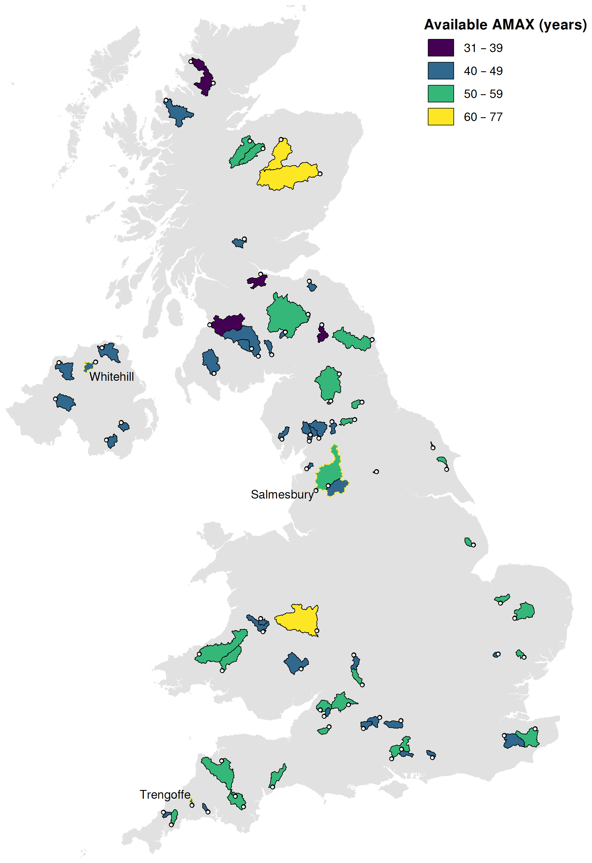
Figure 1Locations of the 73 stations used in the analysis, highlighting record length and location of associated watershed. The three stations considered individually in later figures are labelled and outlined in yellow.
2.2.3 Moving window analysis
To begin, this study uses a moving window analysis, which can be thought of as a window of recent memory. Although it may not be reasonable to assume stationarity over the whole length of a given station's record, it may be reasonable to choose a small window during which there is no statistically significant trend. In particular, the identification of flood-rich or flood-poor periods, as reviewed on a European scale by Hall et al. (2014), may be a strong application for this method.
A fixed-width window of 20 years is applied to each record. The window is moved across the record, year by year, from the start to the end. At each position, stationary GLO parameters are fitted and the value of QMED is computed for only the AMAX data inside the window. This is repeated using a 30-year and 40-year window, for each record that has more years of AMAX data than the width of the window.
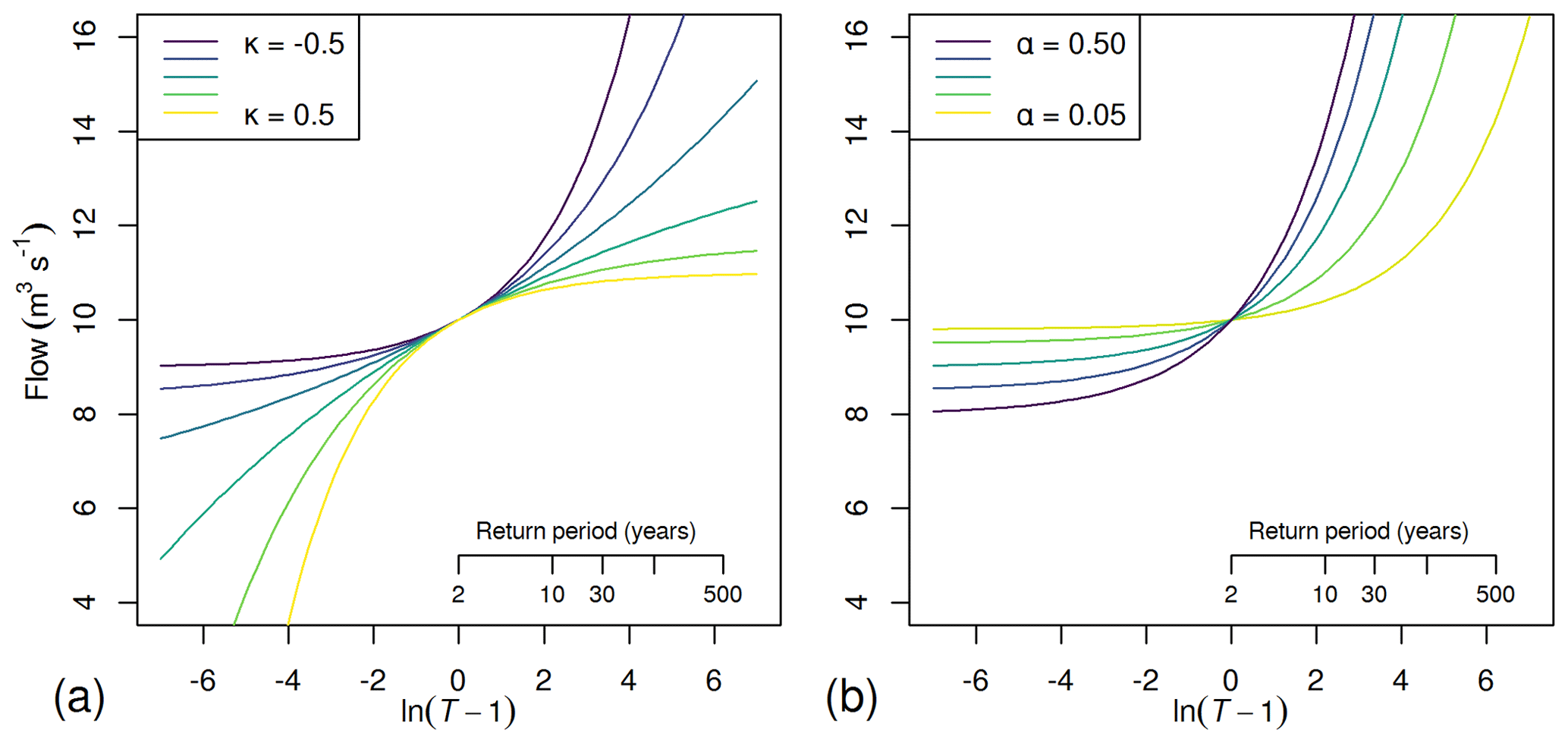
Figure 2Example GLO flood frequency curves. (a) Varying κ, with α=0.5, ξ=10; (b) varying α with κ=0.5, ξ=10. Plotted on logistic reduced variate scale.
2.2.4 Extending window analysis
An alternative approach to analysing the change in flood regime is to adopt an extending window approach, which matches the standard practice of recomputing the flood frequency distribution upon acquiring new data. In the present study, the window initially includes the first 20 years of the record and is extended year by year to eventually cover the whole record. For example, a station for which records start in 1901 would be investigated using windows covering the years 1901–1920, 1901–1921, etc., up to 1901–2016. As before, stationary parameters are fitted and the value of QMED computed at each station using only the data inside the window. The purpose of using extending windows is to see how specific events, once included, affect the values of the stationary parameters and return periods of large events.

Figure 3Example of results from fitting stationary parameters on the Ribble at Samlesbury in different time windows. Parameters (a–c) computed under moving windows, extending windows and on the whole record. AMAX series with QMED moving estimate (e), and flood frequency curves generated from the moving window analysis and from the whole record (d). Note that the value from 1972 to 1973 is missing, but this does not affect the analysis. Lines on figures (a), (b), (c) and (e) are plotted corresponding to the end of the moving or extending windows.
3.1 Moving window analysis
Comparisons between the time series of parameters for the three different window sizes show that wider windows result in more lag (delay in time between the extreme event and an equivalent change in parameters) and attenuation (“smoothing out”) of changes to the parameter estimates as the window is moved. The increased attenuation observed for wider windows is to be expected, as the largest event in a 20-year window has greater weight in parameter calculation than if it were the largest event in a 30- or 40-year window. The increased lag observed for wider windows can be explained as events from further back in the time series taking longer to drop out of the window. However, the width of the window ultimately has little effect on the general overall trends observed. For this reason, only the 20-year window will be used in the rest of this paper to best highlight differences between the start and end of records.
From a hydrological perspective, a distribution based on an AMAX record in which just one event is much larger than QMED (and many smaller) will have strongly negative κ, while a record with several similarly sized events much larger than QMED (and few smaller) will result in a strongly positive κ, which could also suggest a possible maximum flow rate at the station. Hence, for moving window analyses, the change in the shape parameter over time relates to the introduction and, in some cases, later ejection of events either much larger or much smaller than QMED. This can be seen at the end of the example in Fig. 3, where the extreme event (the largest in the record) creates a great change in the moving window estimate of the shape parameter.
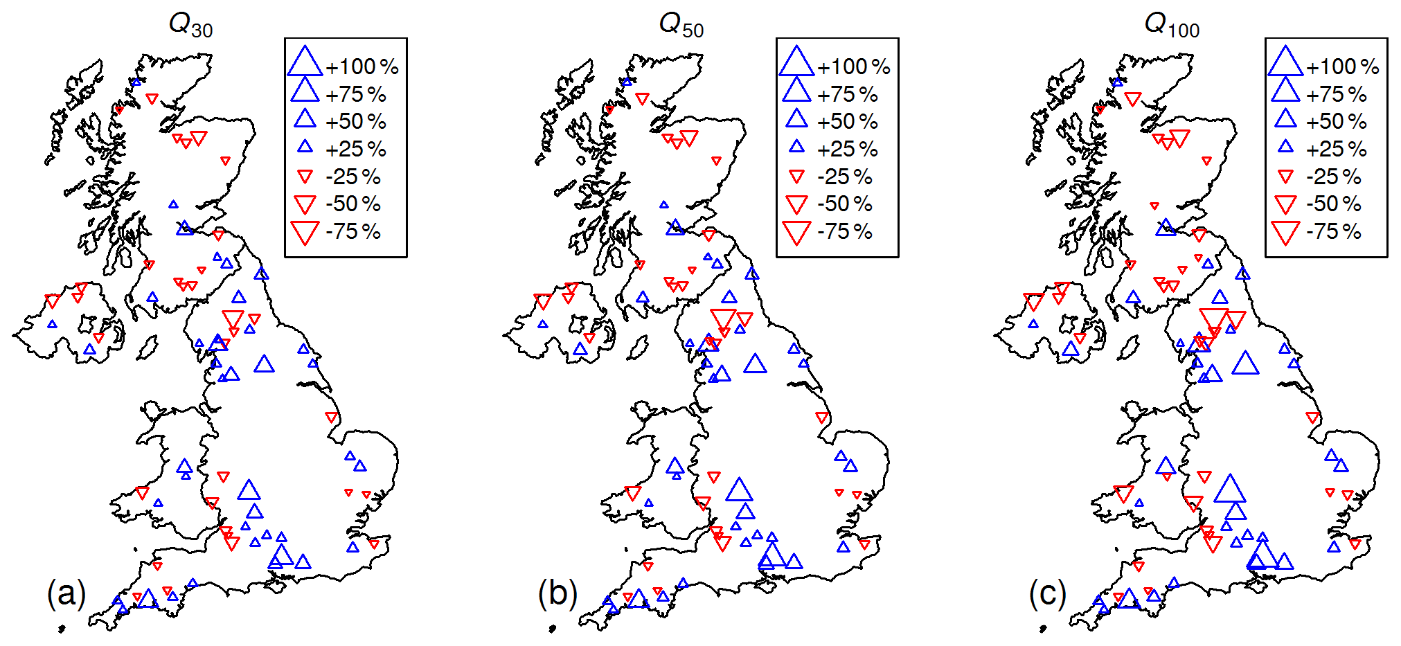
Figure 4Spatial distribution of trends in the 30-, 50- and 100-year return period floods across the UK Benchmark Network, comparing estimates (percentage increase) from the whole record to estimates just using the first 20 years of record at each station.
3.2 Extending window analysis
Trends within extending windows start similarly to those within fixed-width windows but gain an increasing amount of attenuation and lag as older events never drop out of the window. This attenuation and lag means that the flood frequency curves developed for extending windows do not vary as much as for fixed-width windows. Use of an extending window can therefore mask periods of record during which the distribution of AMAX events can be quite different from the average or mask changes in flow regime. However, extraordinary events do still have noticeable effects on the stationary location and shape parameters in particular.
3.2.1 Comparison of moving window and extending window analysis
A typical example of moving window estimates is presented for the Ribble at Samlesbury (NRFA station 71001) in Fig. 3. As a number of large events (bigger than QMED) “drop out of memory”, ξ decreases and κ becomes more extreme, moving away from zero due to the difference between the smallest and largest events in the window. As the big events in 2000 and 2011 appear, the location parameter ξ moves back the other way, whereas the many similarly sized events in this period lead to κ moving towards and eventually passing zero, to become positive again. However, a very extreme event in 2015 leads to a massive shift in the shape parameter, which becomes more negative again.
These changes can be clearly seen in the flood frequency curves (Fig. 3d), where the curves from the middle period are more extreme due to more negative values of κ, but the later curves are more elevated around QMED, where the reduced variate log(T−1) is close to zero, due to large values of ξ. This suggests that Q100 and Q50 estimates decrease towards the end of the record, but Q5 and QMED are increasing towards the end of the record.
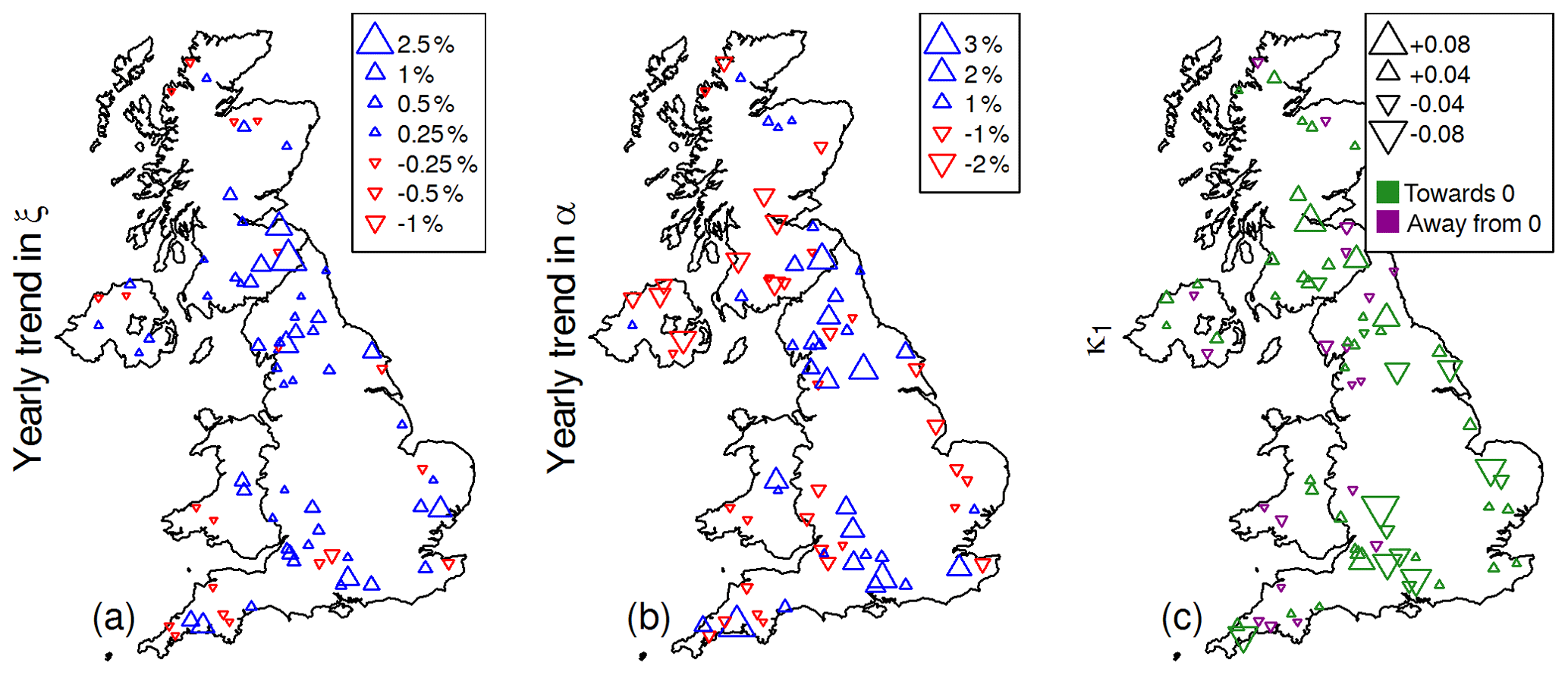
Figure 5Maps of the UK Benchmark Network showing relative spatial trends in ξ (a), α (b), and κ1 (c).
For the extending window analysis, the lengthening record leads to more stable estimates over time. However, variation in estimates can be seen throughout the record, suggesting a lack of convergence to a steady value, particularly in location and shape parameters. Single events such as the low value of 1995 have marked effects. The flood frequency curves under the extending window analysis (not shown) present a similar evolution in flood frequency to that of the moving window, but the curves on the whole show less inter-year variation. The extending window estimate for QMED is still fairly insensitive to the extreme events (both large and small) as records lengthen, even less so than from the moving window; QMED is in many cases chosen over mean annual flood as a primary descriptive statistic for this insensitivity to single extreme events.
3.2.2 Spatial patterns of trends as records lengthen in the UK
To see the effects of using an extending window over the whole of the UK, Fig. 4 demonstrates the difference between using the first 20 years of the record and the whole record for the 30-, 50- and 100-year return period events, corresponding to the 3.33 %, 2 % and 1 % AEP events under stationary conditions. Assuming they come from the same distribution, one might expect little variation between the two estimates (so the percentage difference plotted is close to zero). However, strong differences of up to a 90 % increase have been observed at all three return periods, particularly across England; elsewhere the signal is less clear. Common patterns observed at all long return periods are mostly down to the fixed expression for QT conditional on the parameter values. However, it is seen to be the case that opposite directions of change can be observed at some stations for the 2-year and 5-year events (e.g. Fig. 3).
3.3 Non-stationary analysis
To look at how the stationary estimates compare to the non-stationary ones, parameters that vary in time (ξ(t), α(t), κ(t)) are fitted to the entire record at each station using maximum likelihood estimators.
Across the 73 study catchments, the different types of trend can be divided according to the direction of movement in the median (QMED or ξ increasing or decreasing) and extremes of the flood frequency curve (κ tending towards and away from zero). In some cases, a parameter may reverse its direction of travel one or more times as the window is moved from the start to the end of the record, resulting in a flood frequency curve with an inconsistent time dependency.
Figure 5 shows the size and direction of the parameters ξ1, α1 and κ1 fitted to each of the 73 full AMAX records (i.e. the year-on-year change). The relative changes of location and scale parameters are shown (ξ1∕ξ0, α1), while for κ1 the actual value is shown. Figure 5 confirms that positive trends in the estimates for the location parameter ξ are more numerous and typically larger than negative trends (53 positive vs. 20 negative), and it shows that the largest positive trends cluster around the England–Scotland border, where ξ can increase by 1 %–2.5 % per year.
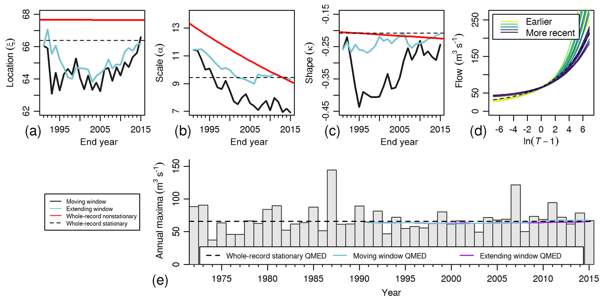
Figure 6Example of results from fitting stationary and non-stationary parameters on the Agivey at Whitehill in different time windows. (a–c) Stationary parameters computed under moving windows, extending windows, and the whole record, and non-stationary parameters computed on the whole record. (e) AMAX series with QMED moving estimate. (d) Flood frequency curves generated from the moving window analysis and generated from the whole record. Lines on figures (a), (b), (c) and (e) are plotted corresponding to the end of the moving or extending windows.
For the scale parameter α, there is less spatial consistency in the size and direction of trends, with 37 positive and 36 negative values of α1. Four positive and no negative trends are greater than 2 %; the most extreme case, α1=0.030, implies that doubles every 23.2 years. The shape parameter α has the greatest influence over the gradient of the flood frequency curve in the centre of the distribution away from the tails, so increased values of α suggest increases in the ratio between magnitudes of more frequent floods (2-year flood and 30-year flood, for example). It should be noted that, to obtain estimates with the same level of uncertainty, a longer AMAX series is required for α1 than for ξ1.
While the magnitudes of κ1 are well balanced on either side of zero, trends towards zero are more numerous than trends away from zero (53 towards vs. 20 away). Smaller values of κ (i.e. closer to zero) have the effect of straightening the flood frequency curve (when return periods are plotted as their logistic reduced variate). This has the effect of reducing the ratios between extreme events (e.g. between the 1 % AEP and 3.33 % AEP floods for a fixed year). It should be noted that an even longer AMAX series is required for a specific level of uncertainty in κ1 than for α1 or ξ1 and that this has been given as a reason in previous studies not to quantify trends in κ (O'Brien and Burn, 2014).
For most records, the overall trend is towards an increase in ξ, corresponding to an increase in QMED and other large floods. However, most stations show a trend in κ whereby its value moves closer to zero. This trend exists for both κ negative and increasing and κ positive and decreasing, and it has the effect of straightening the flood frequency curve: this reduces the ratio between magnitudes of extreme events (e.g. the 1 % AEP and 0.1 % AEP events for a given year) in cases where κ is negative and increasing. The combination thereof confirms the patterns of increasing Q50 and Q100 in Fig. 4.
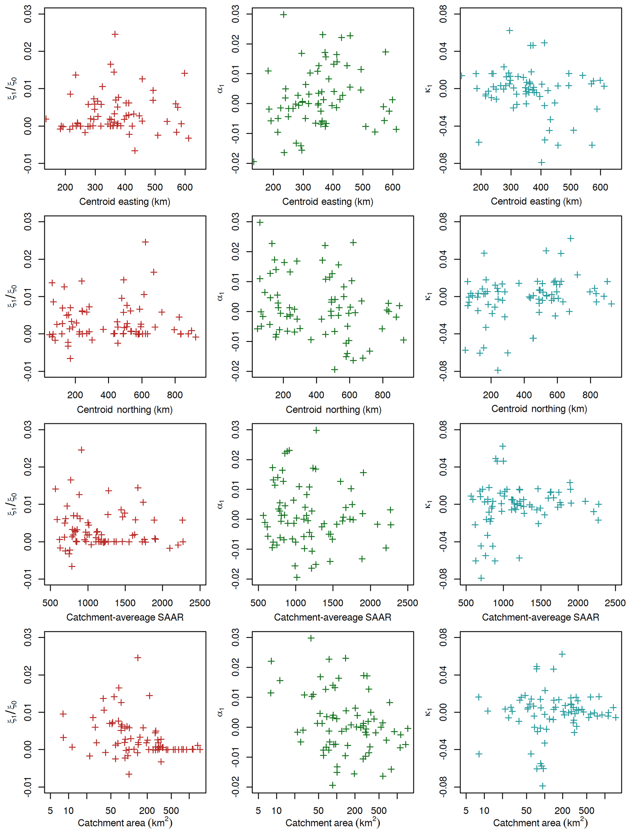
Figure 7Scatterplots plotting catchment descriptors against relative trends in non-stationary parameters.
Although non-stationary parameter fitting over the whole record allows trends to be quantified and compared easily, it can only register the cumulative total trend even if a trend changes direction several times over the period of record. An example of this is demonstrated at Agivey at Whitehill (NRFA station 203028, Fig. 6), where, for a 20-year moving window, κ falls from −0.21 to −0.40 before increasing again to −0.28, corresponding to the occurrence of the largest event in 1987, with the only other similarly large event in 2008. In contrast, for non-stationary parameter fitting, κ changes from −0.21 to −0.23. Although the changes are not consistent over time, a flattening of the flood frequency curve can still be observed, along with a decrease in Q100 (reduced variate of 4.59) despite a steady value of QMED.

Figure 8(a–c) Non-stationary parameters using fixed-start extending windows on the Warleggan at Trengoffe showing change due to addition of single data points, ξ1, α1 and κ1 plotted. (d) AMAX series highlighting period of extending windows.
Although this work does not attempt to attribute causes to the trends in UK peak flow data, it is of interest to see whether any standard covariates correlate strongly with the trends observed. Figure 7 shows the relative change in ξ (ξ1∕ξ0), the relative change in α (α1) and the value of κ1 against catchment centroid easting, catchment centroid northing, average annual rainfall during 1961–1990 (SAAR) and catchment area. This reveals that the strongest negative trends in κ1 are for catchments with SAAR less than about 1000, which are shown to be mostly located in the east of England by co-referencing against the easting and northing subplots. In all cases but one, values of κ1 less than −0.03 correspond to positive values of shape parameter initially decaying towards zero, indicating an increasing upper bound on the flood frequency curve as it straightens. In addition, there are no strong trends in ξ for catchments larger than around 500 km2, and α1 is also potentially shown to be closer to zero for larger catchments. In practical terms, this means that the centre of the flood frequency curve is relatively unchanging over time for larger UK catchments. Nothing else conclusive can be discerned from Fig. 7, potentially as a result of sampling variability causing some catchments to behave in ways that are not typical but still plausible given the record lengths involved.
3.4 Non-stationary extending window analysis
One can also investigate the sensitivity of non-stationary parameters to new data. Starting with the record up to 2000, the non-stationary parameters were refitted for each station after adding one new year at a time. In general, ξ0 and ξ1 changed in opposite directions due to the fact that QMED derived from the whole record (which roughly associates to the average of ξ(t) over the record) varies slowly, but the addition of an extreme point often changes the slope of the fit, so ξ0 has to change conversely to compensate. This is less marked in α(t). In cases where there is low variability in AMAX, the values of κ1, α1 and ξ1 vary slowly, but in many cases these parameters vary erratically.
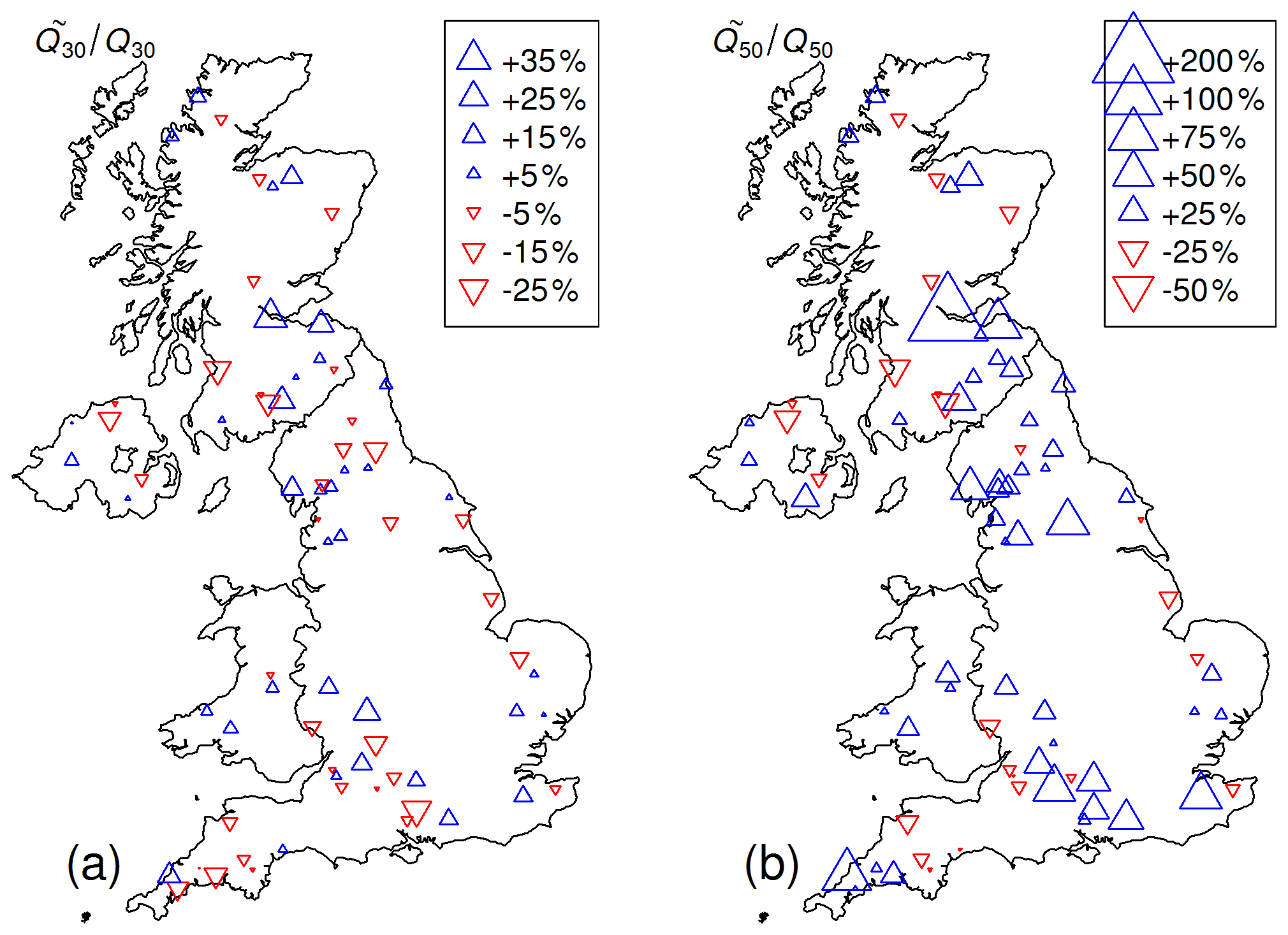
Figure 9Percentage change of long-return-period flood magnitudes computed under assumptions of stationarity (QT) and non-stationary probability of exceedance (. Shown for the 30-year event (a) and 50-year event (b).
Figure 8 shows an example where the presence of an extreme event massively changes the trend parameters. The event in 2010, which far exceeds any previous event, has a very large effect on κ1 and α1, causing both to become significantly more negative. Compare this to the relatively smooth variation before 2006 which could be linked to the very consistent values of AMAX close to QMED in 2000–2006, which would lead to an increase in κ(t) and drop in α(t), and push ξ1 closer to zero. It should be noted, though, that this example is extremely clear, most stations showed similar effects but with much more variability.
3.5 Changes in flood return periods
Finally the 30-year and 50-year floods are compared for each of the stations with records extending up to at least 2015, under stationary and non-stationary estimates. The values of Q30 and Q50 are computed from the stationary parameter estimates. Then, using the non-stationary parameter estimates, the annual probabilities of exceedance PQ(y) are computed. These are used to find the return period function TQ as in Sect. 3.3.2. and , with y0 equal to the start of each station's record, are then computed by inverting the function. Note that, for numerical tractability, the sum was truncated once the value of summands became less than 0.01. The values obtained were tested and seen to be fairly insensitive to the exact threshold for truncation, as long as it was sufficiently small (much less than 1).
Figure 9 shows the ratios of and . Note that if these changes are greater than zero, then this suggests that the event under non-stationary assumptions is larger. In general, we see a quite mixed signal for the 30-year event, suggesting that many of these estimates are quite similar under stationary and non-stationary assumptions. However, for the 50-year event we see a more consistent increase in magnitude compared to estimates made under stationary assumptions at the start of the period of record. This is likely due to the continued increase in location and scale parameters over time (compare to Fig. 5), causing an ever-increasing discrepancy between the stationary and non-stationary probabilities of exceedance. As in Fig. 5, the biggest changes are around the England–Scotland border. On the whole, however, it seems as though increases in location (ξ) and scale (α) have a bigger impact than the decrease in the absolute value of the shape (κ). This can be observed in the increases in Q50 and Q100 across the region.
In this paper, the updated UK Benchmark Network has been used as a near-natural set of example stations to investigate how the inclusion of new data affects flood frequency estimates, as well as the underlying distribution parameters under stationary and non-stationary models.
In a stationary setting, examples of parameters changing over time, using an extending window of record, highlight the fact that the addition of single large events can drastically change parameter estimates, forcing more extreme values of location and shape. Even in the non-stationary setting, the inclusion of new events can greatly shift the slope in all parameters, as the maximum likelihood estimation (MLE) method has to refit the entire slope to account for this one point.
When non-stationarity is included in the flood frequency model, the main spatial trends observed are consistent patterns in increasing location parameters and shape parameters moving towards zero, though an investigation into catchment descriptors identified no significant correlation. However, some slight patterns were observed regarding links between changes in location and scale parameter and area of catchment, as well as between shape parameter and average annual rainfall (SAAR) or geographical location. The uncertainty associated with this will be the focus of future work.
Leading on from the parameter variability, flood frequency curves can be strongly influenced by the introduction of new points, especially if a moving window approach is used. The change in the 2-year flood behaviour by the addition of larger and smaller events was reaffirmed, but this event was seen to be more robust to the addition of new data than the more extreme events. Flood frequency curves may be flattening in many places, suggesting that the most extreme floods may not necessarily be getting bigger relative to the 2-year flood but that the more likely floods, such as the 5-year flood, may be getting larger. This agrees with Hirsch and Archfield (2015), which showed that the addition of single events was enough to have a marked difference in the estimates of, for example, Q50 and Q100. Switching from stationary to nonstationary models was also seen to have a marked difference, especially in long return periods.
On the whole, the inclusion of non-stationarity allows, in some sense, the ability to exchange variability (which leads to more extreme scale and shape parameters) for change over time, which can lead to less extreme flood frequency curves overall. When deciding whether to include a new data point, unprecedented events should not be discarded, but close inspection of the change in flood frequency estimates should be undertaken to determine whether this is a symptom of changing flood regimes which may be better described using a non-stationary model.
As mentioned in Sect. 3.5, an increase in long-return-period events is observed despite a drop in the shape parameter towards zero. This is due to the overall increase in location and scale parameters over time. In some cases, correlation between change in scale and change in shape could be linked to the addition of a single large event. A full systematic investigation of this correlation would likely be interesting to undertake.
It should be noted that the choices of non-stationary functions for the GLO parameters made in this paper are not the only options. Aside from the inclusion of other covariates besides time, which is an important question in itself, the choice of transformation of time can make a difference. It has been discussed in the literature (O'Brien and Burn, 2014) and could be the source of more dedicated analysis.
In the future, the use of fixed-width moving windows would be very valuable in the study of flood-rich/flood-poor period quantification in river flow data. If these periods can be elucidated, it would be of interest to examine the underlying hydrological mechanisms. On a shorter timescale, the moving window approach could offer some insight into seasonality modelling in flood frequency estimation.
The data were all obtained freely from the National River Flow Archive (version 6: 2017).
ES coordinated the study, helped write the manuscript and added context to the research. GV generated all the figures and helped write the manuscript. AG designed and performed the analysis and helped write the manuscript.
The authors declare they have no conflict of interest.
The authors would like to thank Giuseppe Formetta and Chingka Kalai as well as the editors and reviewers for their invaluable feedback. This work was funded by the Centre for Ecology & Hydrology through the FEH research programme and through national capability funding within the Hydro-climate Risks science area.
This paper was edited by Vassiliki Kotroni and reviewed by Ilaria Prosdocimi and one anonymous referee.
Barker, L., Hannaford, J., Muchan, K., Turner, S., and Parry, S.: The winter 2015/2016 floods in the UK: a hydrological appraisal, Weather, 71, 324–333, https://doi.org/10.1002/wea.2822, 2016.
Coles, S: An Introduction to Statistical Modelling of Extreme Values, Springer Series in Statistics, Springer London, London, 2001.
Collet, L., Harrigan, S., Prudhomme, C., Formetta, G., and Beevers, L.: Future hot-spots for hydro-hazards in Great Britain: a probabilistic assessment, Hydrol. Earth Syst. Sci., 22, 5387–5401, https://doi.org/10.5194/hess-22-5387-2018, 2018.
Cunderlik, J. M. and Burn, D. H.: Non-stationary pooled flood frequency analysis, J. Hydrol., 276, 210–223, https://doi.org/10.1016/S0022-1694(03)00062-3, 2003.
Defra: National Flood Resilience Review, UK Government, London, 2016.
Eastoe, E. F.: Nonstationarity in peaks-over-threshold river flows: A regional random effects model, Environmetrics, e2560, https://doi.org/10.1002/env.2560, 2019.
Hall, J., Arheimer, B., Borga, M., Brázdil, R., Claps, P., Kiss, A., Kjeldsen, T. R., Kriaučiūnienė, J., Kundzewicz, Z. W., Lang, M., Llasat, M. C., Macdonald, N., McIntyre, N., Mediero, L., Merz, B., Merz, R., Molnar, P., Montanari, A., Neuhold, C., Parajka, J., Perdigão, R. A. P., Plavcová, L., Rogger, M., Salinas, J. L., Sauquet, E., Schär, C., Szolgay, J., Viglione, A., and Blöschl, G.: Understanding flood regime changes in Europe: a state-of-the-art assessment, Hydrol. Earth Syst. Sci., 18, 2735–2772, https://doi.org/10.5194/hess-18-2735-2014, 2014.
Hannaford, J. and Marsh, T.: An assessment of trends in UK runoff and low flows using a network of undisturbed catchments, Int. J. Climatol., 26, 1237–1253, https://doi.org/10.1002/joc.1303, 2006.
Harrigan, S., Hannaford, J., Muchan, K., and Marsh, T. J.: Designation and trend analysis of the updated UK Benchmark Network of river flow stations: The UKBN2 dataset, Hydrol. Res., 49, 552–567, https://doi.org/10.2166/nh.2017.058, 2018.
Hirsch, R. M. and Archfield, S. A.: Not higher but more often, Nat. Clim. Change, 5, 198–199, https://doi.org/10.1038/nclimate2551, 2015.
Hosking, J. R. M. and Wallis, J. R.: Regional Frequency Analysis, Cambridge University Press, Cambridge, 1997.
Hu, Y., Liang, Z., Singh, V. P., Zhang, X., Wang, J., Li, B., and Wang, H.: Concept of Equivalent Reliability for Estimating the Design Flood under Non-stationary Conditions, Water Resour. Manag., 32, 552–567, https://doi.org/10.1007/s11269-017-1851-y, 2018.
IPCC: Climate Change 2013 – The Physical Science Basis, Intergovernmental Panel on Climate Change, Climate Change 2013: The Physical Science Basis., Contribution of Working Group I to the Fifth Assessment Report of the Intergovernmental Panel on Climate Change, Cambridge University Press, Cambridge, https://doi.org/10.1017/CBO9781107415324, 2014.
Johannesson, Á. V., Hrafnkelsson, B., Huser, R., Bakka, H., and Siegert, S. Approximate Bayesian inference for spatial flood frequency analysis, arXiv preprint, arXiv:1907.04763, 2019.
Kay, A. L. and Jones, D. A.: Transient changes in flood frequency and timing in Britain under potential projections of climate change, Int. J. Climatol., 32, 489–502, https://doi.org/10.1002/joc.2288, 2012.
Kjeldsen, T. R. and Prosdocimi, I.: Assessing the element of surprise of record-breaking flood events, J. Flood Risk Manag., 11, S541–S553., https://doi.org/10.1111/jfr3.12260, 2018.
Leclerc, M. and Ouarda, T. B. M. J: Non-stationary regional flood frequency analysis at ungauged sites, J. Hydrol., 343, 254–265, https://doi.org/10.1016/j.jhydrol.2007.06.021, 2007.
Marsh, T. J., Kirby, C., Barker, L., Henderson, E., and Hannaford, J.: The winter floods of 2015/2016 in the UK – a review, Centre for Ecology & Hydrology, Wallingford, 2016.
NRFA: National River Flow Archive, available at: http://nrfa.ceh.ac.uk/data, last access: 20 November 2018.
O'Brien, N. L. and Burn, D. H.: A non-stationary index-flood technique for estimating extreme quantiles for annual maximum streamflow, J. Hydrol., 519, 2040–2048, https://doi.org/10.1016/j.jhydrol.2014.09.041, 2014.
Prosdocimi, I., Kjeldsen, T. R., and Svensson, C.: Non-stationarity in annual and seasonal series of peak flow and precipitation in the UK, Nat. Hazards Earth Syst. Sci., 14, 1125–1144, https://doi.org/10.5194/nhess-14-1125-2014, 2014.
Reynard, N. S., Kay, A. L., Anderson, M., Donovan, B., and Duckworth, C.: The evolution of climate change guidance for fluvial flood risk management in England, Prog. Phys. Geog., 41, 222–237, https://doi.org/10.1177/0309133317702566, 2017.
Robson, A. J. and Reed, D. W.: Statistical procedures for flood frequency estimation, Flood Estimation Handbook (Vol. 3), Institute of Hydrology, Wallingford, 1999.
Salas, J. D. and Obeysekera, J.: Revisiting the Concepts of Return Period and Risk for Non-stationary Hydrologic Extreme Events, J. Hydrol. Eng., 19, 554–568, https://doi.org/10.1061/(ASCE)HE.1943-5584.0000820, 2014.
Spencer, P., Faulkner, D., Perkins, I., Lindsay, D., Dixon, G., Parkes, M., Lowe, A., Asadullah, A., Hearn, K., Gaffney, L., Parkes, A., and James, R.: The floods of December 2015 in northern England: description of the events and possible implications for flood hydrology in the UK, Hydrol. Res., 49, 568–596, https://doi.org/10.2166/nh.2017.092, 2018.