the Creative Commons Attribution 4.0 License.
the Creative Commons Attribution 4.0 License.
 | 24 Oct 2018
Combining probability distributions of sea level variations and wave run-up to evaluate coastal flooding risks
Jan-Victor Björkqvist
Milla M. Johansson
Havu Pellikka
Lauri Laakso
Kimmo K. Kahma
Tools for estimating probabilities of flooding hazards caused by the simultaneous effect of sea level and waves are needed for the secure planning of densely populated coastal areas that are strongly vulnerable to climate change. In this paper we present a method for combining location-specific probability distributions of three different components: (1) long-term mean sea level change, (2) short-term sea level variations and (3) wind-generated waves. We apply the method at two locations in the Helsinki archipelago to obtain total water level estimates representing the joint effect of the still water level and the wave run-up for the present, 2050 and 2100. The variability of the wave conditions between the study sites leads to a difference in the safe building levels of up to 1 m. The rising mean sea level in the Gulf of Finland and the uncertainty related to the associated scenarios contribute notably to the total water levels for the year 2100. A test with theoretical wave run-up distributions illustrates the effect of the relative magnitude of the sea level variations and wave conditions on the total water level. We also discuss our method's applicability to other coastal regions.
- Article
(1589 KB) - Full-text XML
-
Supplement
(3566 KB) - BibTeX
- EndNote


Predicting coastal flooding and extreme sea level events has a focal role in the designing of rapidly evolving coastal areas, which are continuously more populated and convoluted. Such flooding events are influenced by long-term changes in mean sea level, together with short-term sea level variations and the wind-generated wave fields. These processes are further influenced by a variety of other processes and conditions like vertical crustal movements, islands, the shape of the shoreline and the topography of the seabed. Because of a rising mean sea level, the effect of sea level variations accompanied by waves might cause more damage in the future than in the present conditions. In this study, we analyse the joint effect of the still water level and wind waves on the Finnish coast.
Globally, several studies have addressed the topic of combining sea level changes and variations with wind waves in different circumstances and at different locations, using different methods and assumptions. Hawkes et al. (2002) studied the combined effect of large waves and high still water in coastal areas of England and Wales using Monte Carlo simulations, accounting for the dependence between the water level, the wave height and the wave steepness. Hawkes (2008) summarised joint probability methods and discussed issues related to data selection and event definition, concluding that the analysis method and source data should be well chosen to meet the requirements of a particular problem.
Wahl et al. (2012) applied Archimedean copula functions in the German Bight to achieve exceedance probabilities for storm surges and wind waves. They found that, when this methodology is used, realistic exceedance probabilities can be achieved and used to enhance the results from integrated (i.e. multivariate problems) flood risk analyses. A copula-based approach was also implemented by Masina et al. (2015) to examine the joint distribution of sea level and waves at a location suffering from coastal flooding in northern Italy (Ravenna coast). This method accounts for the dependence structure between the variables, and the authors also assessed the present probability of marine inundation, accounting for the interrelationship among the main sea condition variables and their seasonal variability. Results of this study highlight the need to utilise all variables and their dependences simultaneously in order to obtain realistic estimates for flooding probabilities.
In a study conducted by Prime et al. (2016), the authors used a combination of a storm impact model and a flood inundation model to quantify the uncertainty in flood depth and extent of a 0.5 % probability event in the Dungeness and Romney Marsh coastal zone in the UK. They found that the most significant flood hazards at their study site were caused by low swell waves during the highest water levels, as opposed to large wind waves occurring at lower water levels. Chini and Stansby (2012) used an integrated modelling system to investigate the joint probability of extreme wave height and water level at Walcott on the eastern coast of the UK, thus determining changes in overtopping rates. Using different scenarios for the mean sea level rise, the authors found that flooding probabilities are mainly influenced by changes in water level, as opposed to changes in the waves conditions. Cannaby et al. (2016) reached a similar conclusion when studying coastal flooding risks in the Singapore region.
Although the changes in water level have been deemed to have the highest impact on flooding risks by several authors, Chini et al. (2010) found the near-shore wave conditions on the East Anglia coast (UK) to be sensitive to the changes in water level. The authors used five linear sea level rise scenarios and one climatic scenario for storm surges and offshore waves to study the waves between 1960 and 2099. Cheon and Suh (2016) also found that the depth limitation of waves can be relaxed with increasing mean sea level, thus leading to increased risks for wave-induced damages on inclined coastal structures.
The Baltic Sea is a shallow semi-enclosed marginal sea, connected to the Atlantic Ocean only through the narrow and shallow Danish Straits. This gives the sea level variations in the Baltic Sea a unique nature, which differs from that on the ocean coasts. The components of local sea level variations on a short timescale include wind waves, wind- and air-pressure-induced sea level variations, currents, tides, internal oscillation (seiche) and meteotsunamis. Long-term changes are related to the climate-change-driven mean sea level variations; postglacial land uplift; and the limited exchange of water through the Danish Straits, which causes variations up to 1.3 m in the average level of the Baltic Sea on a weekly timescale (Leppäranta and Myrberg, 2009; Pellikka et al., 2014; Johansson et al., 2014).
Both sea level and wind waves have been thoroughly studied separately in the Baltic Sea area, but research into their joint effect is sparse compared to coastal regions outside the Baltic Sea. Hanson and Larson (2008) examined jointly waves and water levels to estimate run-up levels (as the sum of the mean water level and the wave run-up height) on the Swedish coast in the southern Baltic Sea. They established probability distributions based on existing climate data (mainly wind and water level data) also including scenarios of future climate change. On the Estonian coast in the Gulf of Finland the impact of breaking waves on the mean water level (wave set-up) was studied by Soomere et al. (2013), who found, based on results from a numerical wave model, the wave set-up to be strongly affected by the wind direction. Pindsoo and Soomere (2015) reached the same conclusion in a study that also accounted for varying offshore water level variations simulated by the Rossby Centre Ocean (RCO) model.
In Finland, there is a clear demand for flooding risk evaluation. The irregular coastline is characterised by coastal archipelagos consisting of tens of thousands of islands. Especially the southern part of the coast will likely become exposed to increasing flooding risks, as the land uplift rate no longer compensates for the accelerating sea level rise (Pellikka et al., 2018).
During the record-breaking storm Gudrun in 2005, three different components acted simultaneously in the Gulf of Finland: a high total water amount in the Baltic Sea, a high phase of the standing waves (seiches), and severe winds piling up the water and waves towards the shore. Gudrun caused major damage to coastal infrastructure on both the north and south sides of the Gulf of Finland (Parjanne and Huokuna, 2014; Tõnisson et al., 2008; Suursaar et al., 2006).
The earlier flooding risk estimates in Finland (Kahma et al., 1998, 2014; Pellikka et al., 2018) were based on combining the probability distributions of the observed short-term sea level variability and the long-term mean sea level projections (Johansson et al., 2014). On top of these estimates, a location-specific additional height for wind waves (henceforth “wave action height”) was accounted for separately.
In this study, we utilise location-specific probability distributions of water level and wave run-up to obtain a single probability distribution for the maximum absolute elevation of the continuous water mass (Fig. 1). For simplicity, we call this resulting elevation the total water level. The method presented in this paper has been applied to assess the safe building heights on the coast of Helsinki (Kahma et al., 2016).
This paper is structured in the following manner. In Sect. 2, we outline the parameters affecting the sea surface level on the Finnish coast. In Sect. 3, we introduce the scenarios and observations used in this study. This is continued in Sect. 4 by forming the sea level and wave probability distributions, presenting the theory for evaluating the sum of two random variables and the particulars of applying it to sea level variations and wind waves. In Sect. 5 we apply the method on a case study in the Helsinki archipelago and beside it investigate theoretically how different wave height conditions affect the resulting total water level. The paper is finished by discussion on the relevance and applicability of the results in Sect. 6, and finally conclusions in Sect. 7.
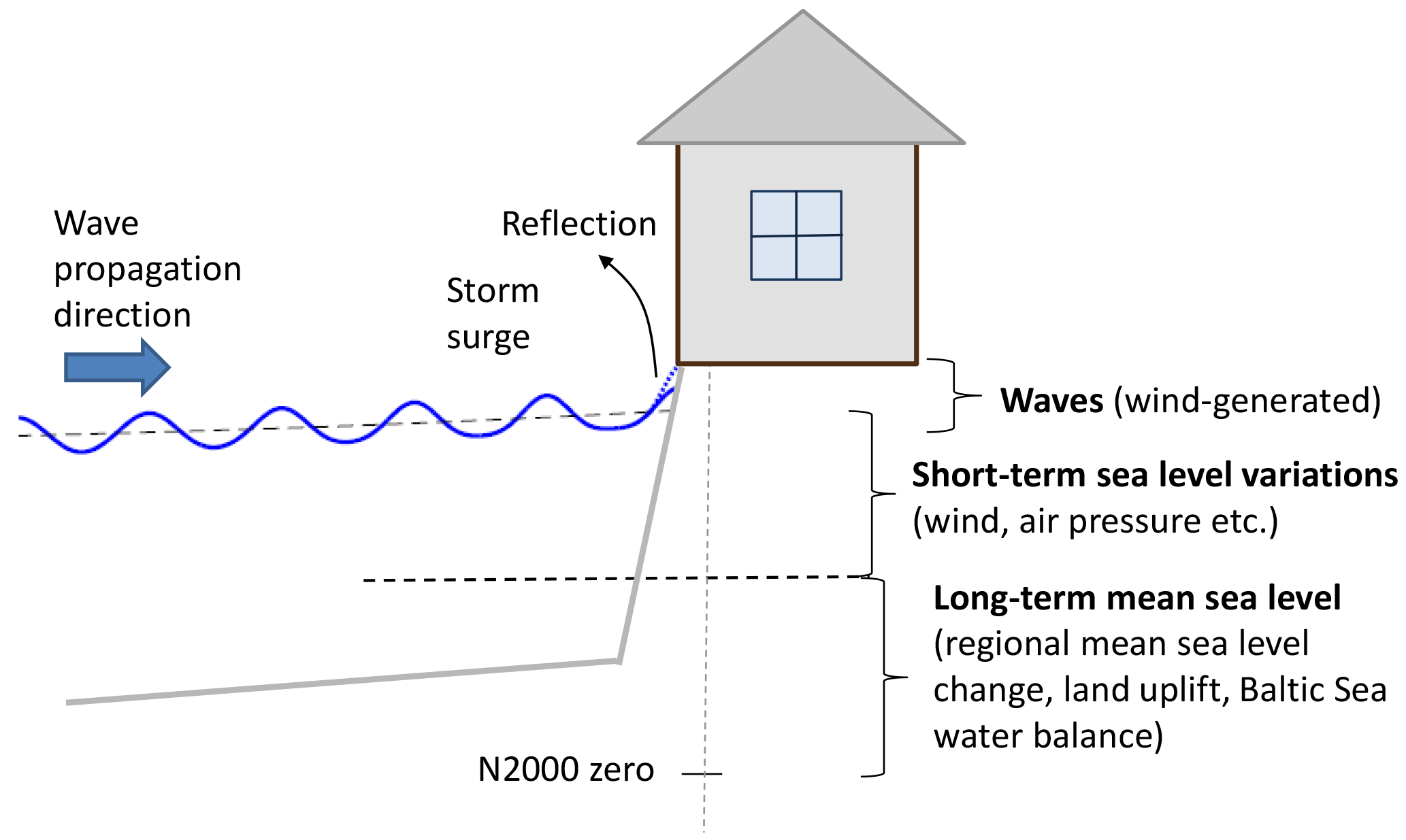
Figure 1The total water level, i.e. the maximum absolute elevation of the continuous water mass (solid blue), is a result of the (1) long-term mean sea level change, (2) short-term sea level variations and (3) wind-generated waves. On a steep shore the waves can also be fully or partially reflected (dotted blue).
The instantaneous sea surface height at any coastal site in the Baltic Sea is affected by several physical processes on different timescales. In this study, we use the term still water level to represent the maximum elevation of the water level (including short- and long-term sea level variations). Moreover, we use the term total water level H to represent the maximum absolute elevation of continuous water mass as a sum of three components with different timescales (Fig. 1):
where SL stands for the long-term sea level, SS for the short-term sea level variations and Hrunup for the wave run-up above the still water level (SL+SS).
The long-term mean sea level on the Finnish coast, on decadal timescale, is affected by the global mean sea level, the postglacial land uplift and the Baltic Sea water balance (Johansson et al., 2014). The global mean sea level is rising due to thermal expansion of sea water and melting of glaciers and ice sheets. Nevertheless, the rising sea level is locally mitigated by the postglacial land uplift, which presently amounts to 3–10 mm yr−1 on the Finnish coast. The mean sea level in the Baltic Sea can also deviate from the mean ocean level because of the limited water exchange through the narrow and shallow Danish Straits, which connect the Baltic Sea to the North Atlantic Ocean. The in- and outflow of water through the Danish Straits are mainly driven by the regional wind and air pressure conditions, while other factors such as river runoff, evaporation and precipitation have a negligible effect on the Baltic Sea water balance.
Short-term sea level variations on a sub-decadal timescale on the Finnish coast range from −1.3 to +2.0 m above the long-term mean sea level, with timescales ranging from year-to-year variability of the Baltic Sea total water volume down to storm surges and other rapid variations in less than an hour. The week-to-week variability of the water volume results in a sea level variability of about 1.3 m, while the shorter-period internal variations in the Baltic Sea basin contribute several tens of centimetres to the sea level variability (Leppäranta and Myrberg, 2009). Along the Finnish coast, the largest variations occur near the closed ends of the Bay of Bothnia and Gulf of Finland, while the range of variability at sites closer to the central area of the Baltic Sea is substantially smaller (e.g. Johansson et al., 2001). These variations are mainly driven by wind and air pressure variations. Ice conditions in the winter also affect the water level variability, but, unlike in many other coastal areas, the tidal variations range only up to 10–15 cm on the Finnish coast (Witting, 1911; Leppäranta and Myrberg, 2009; Särkkä et al., 2017).
The wave conditions in the Baltic Sea are influenced by the limited fetch, the topography of the seabed and the seasonal ice cover (Tuomi et al., 2011). The highest observed significant wave height in the Baltic Sea is 8.2 m (Björkqvist et al., 2017b). In the Gulf of Finland the growth of the waves is restricted by the narrowness of the gulf (Kahma and Pettersson, 1994), but a significant wave height of 5.2 m has still been measured in the centre of the Gulf of Finland (Pettersson et al., 2013). Close to the shoreline the waves are modified by the archipelago and the irregular shoreline (Tuomi et al., 2014; Björkqvist et al., 2017a). The significant wave height close to the coast in the Helsinki archipelago has been estimated to not exceed 2 m (Kahma et al., 2016), but the steep shoreline near Helsinki causes wave reflection leading to a positive interference (Björkqvist et al., 2017c). This reflection affects the wave run-up, which is the vertical elevation that the continuous water mass reaches with respect to the still water level.

Figure 2The coastal area off Helsinki and the measurement sites used in the study. The red box in the Baltic Sea map (a) marks the area shown in (b). The circles mark the location of the moored wave buoys, and the star represents the Helsinki tide gauge used to collect the sea level data. The contours mark the approximate water depth.
3.1 Long-term mean sea level: past estimate and future scenarios
We focused our calculations on three different years: 2017, 2050 and 2100. Pellikka et al. (2018) calculated estimates for the past long-term mean sea level, as well as future scenarios, on the Finnish coast. They estimated the past and present long-term mean sea level as a combination of the past actualised global sea level rise, land uplift and Baltic Sea water balance. The significant year-to-year variability in the Baltic Sea water balance was smoothed out by a 15-year floating average.
The future scenarios of Pellikka et al. (2018) were based on an ensemble of 14 global mean sea level rise projections from the recent scientific literature. Each projection was adjusted to the Finnish coast by taking into account the uneven geographical distribution of the thermal expansion of sea water, ocean dynamical changes and the fingerprints of the melting ice masses. The regionalised projections, along with their uncertainties, were combined to obtain a probability distribution of the sea level rise in 2000–2100. Lastly, these localised sea level rise scenarios were combined with the postglacial land uplift and an estimate of wind-induced changes in the Baltic Sea water balance. For more details of the method, see Johansson et al. (2014) and Pellikka et al. (2018). In Helsinki, the change in mean sea level in 2000–2100 was projected to be 30 cm (−15 to +87 cm, 5 %–95 % uncertainty range).
3.2 Sea level data
The Finnish Meteorological Institute (FMI) operates 14 tide gauges along the Finnish coast, most of which have been operating since the 1920s. We used 46 years (1971–2016) of instantaneous hourly sea level observations from the Helsinki tide gauge. The Finnish sea level data are measured in relation to a tide-gauge-specific fixed reference level, which is regularly levelled to the height system N2000. The height system N2000 is a Finnish realisation of the common European height system. The N2000 datum is derived from the NAP (Normaal Amsterdams Peil; Saaranen et al., 2009). For a more detailed description of the tide gauge data, measurement techniques and quality, see Johansson et al. (2001).
The sea level variations are location-specific, but, as our study area is limited to sites less than 5 km away from the Helsinki tide gauge, we considered the sea level variability measured at the tide gauge sufficiently representative for both study sites at Jätkäsaari and Länsikari (Fig. 2).
3.3 Wind wave data
FMI conducts operational wind wave measurements at four locations in the Baltic Sea. In the Gulf of Finland, the observations are carried out using a Datawell Directional Waverider moored in the centre of the gulf (see Fig. 2). However, these open-sea observations are not representative of nearshore wave conditions (e.g. Kahma et al., 2016; Björkqvist et al., 2017a). The operational measurements have therefore been supplemented by short-term observations with smaller Datawell G4 wave buoys inside the Helsinki archipelago.
We used the open-sea measurements from the operational Gulf of Finland wave buoy in 2000–2014 in combination with shorter time series at chosen locations inside the Helsinki coastal archipelago. The measurements in the archipelago were conducted at Jätkäsaari (31 days in October 2012) and Länsikari (11 days in November 2013) (see Fig. 2). These shorter measurements were a part of a research project commissioned by the City of Helsinki (Kahma et al., 2016).
We chose the measurement sites at Jätkäsaari and Länsikari so that they would represent two different kinds of wave conditions: Jätkäsaari is close to the shore, in a place well sheltered from the open sea by islands. Länsikari, on the other hand, is located in the outer archipelago, relatively unsheltered from the open-sea conditions.
Most wave parameters can be defined using spectral moments:
where S(f) is the variance density spectrum (m2Hz−1) given as a function of the wave frequency. The significant wave height can then be calculated as
The wave period Tm02 is defined as
As a first step in estimating the combined effect of the long-term mean sea level, the short-term sea level variability and the wind waves on the frequencies of exceedance of coastal floods, we constructed probability distributions for each of them separately (Sect. 4.1–4.3). Next, we calculated the probability distributions of their sum: the method for this is presented in Sect. 4.4 and applied on the three constructed distributions in Sect. 4.5.
In this paper, we use three types of probability distributions. The probability density function (PDF) fx, the cumulative distribution function (CDF) Fx and the complementary cumulative distribution function (CCDF) of the random variable are defined as
Since our data are based on hourly values, we converted the frequencies of exceedance from the CCDF to events per year by multiplying them with the average number of hours per year (8766). By using hourly sea level values, we practically assume a constant sea level for the entire hour. When summing a 1 h constant sea level value with a 1 h maximum wave run-up with respect to the mean water level, the result is the maximum absolute elevation within 1 h. This maximum absolute elevation during 1 h is defined as one event.
4.1 Distributions of the long-term sea level scenario
The probability distributions for the long-term mean sea level scenarios on the Finnish coast were calculated by Pellikka et al. (2018). We used their PDFs for sea level scenarios at Helsinki in 2050 and 2100, and the long-term mean sea level estimate of 0.19 m for the year 2017 in reference to the N2000 height system (Fig. 3). The medians of these scenarios project a rise of 0.04 m from the estimated mean sea level of 2017 up to 2050 and a rise of 0.27 m from 2017 to 2100. The uncertainties, however, increase markedly in the future, with the width of the 5 % to 95 % range of the CDF being 0.37 m in 2050 and 1.03 m in 2100.
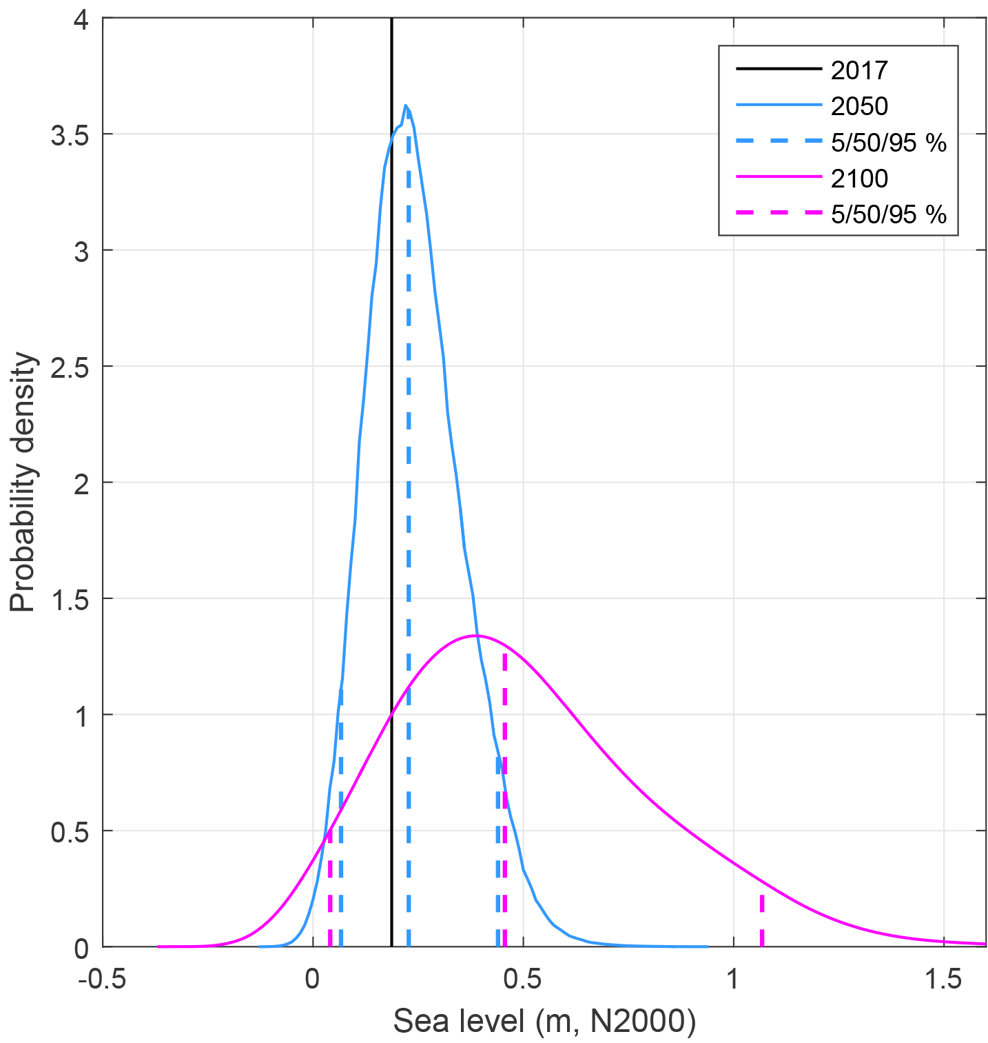
Figure 3Probability density functions of future mean sea level at the Helsinki tide gauge for the years 2050 and 2100 and the long-term mean sea level estimate of 0.19 m for the year 2017. The 5th, 50th and 95th percentiles are shown for 2050 and 2100. The data in the figure are from the results of Pellikka et al. (2018).
4.2 Distribution of the short-term sea level variability
We constructed the probability distribution of short-term sea level variability from the observed sea levels in 1971–2016. The observed sea levels practically represent the sum of the first two terms of Eq. (1). We subtracted the annual values of the past long-term variations (SL; see Sect. 3.1) from the observed time series to obtain the short-term variability SS.
We then calculated the CCDF for the short-term sea level variations and extrapolated it with an exponential function (Fig. 4). The exponential function was fitted to the tail of the CCDF, to sea levels with a frequency of exceedance less than , which corresponds to 5 h yr−1. This limit was selected because only the tail part of the distribution follows the exponential shape, while more frequent sea levels behave differently. Särkkä et al. (2017) examined different functions and methods for extrapolating sea level CCDFs at Helsinki. They found that both a Weibull and an exponential extrapolation of simulated daily sea level maxima produced results well in line with a generalised extreme value (GEV) fit to simulated annual sea level maxima.
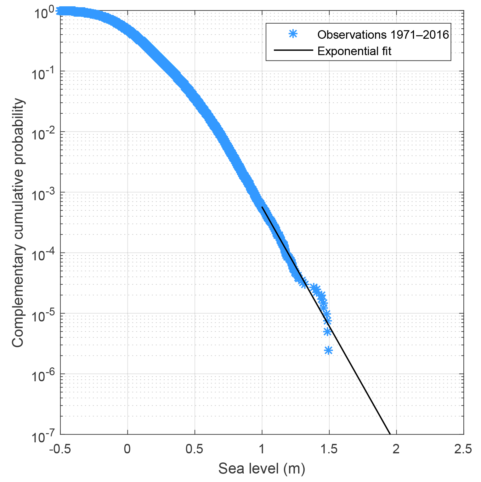
Figure 4CCDF of the short-term sea level variations at the Helsinki tide gauge: observed hourly values in 1971–2016, from which a time-dependent estimate for the long-term mean sea level has been subtracted.
4.3 Distributions of the wind wave run-up
4.3.1 Observed distributions
The short time series measured at Jätkäsaari and Länsikari (Sect. 3.3) are not long enough for constructing the local wave height probability distributions. We therefore compared these measurements to the simultaneous open-sea data from the Gulf of Finland to determine an attenuation factor for each wave direction and wave period. The attenuation factors were then applied to the 15-year open-sea measurement record to produce estimates of the wave conditions at the study locations. We calculated hourly significant wave heights from two consecutive measured 30 min values, to be able to combine these with the hourly sea level data.
The wave height values obtained by attenuating the open-sea data were combined with the local measurements, and CCDFs were estimated by fitting piecewise exponential functions to the data. For the large values of the CCDF the exponential function was fitted to the observational data, while for the smaller values (rarer events) a fit was made to the modelled values. These two pieces were connected to form one continuous distribution (see Fig. 6). The distribution was then extrapolated using an exponential fit. Since neither the observations nor the modelled values are by themselves sufficient to form a probability distribution, the above method was chosen to make the most efficient use of both data sets.
The final step was to estimate the wave run-up, i.e. the maximum vertical elevation of the water in relation to the still water level. We defined the wave run-up using the highest single wave during an hour, since this will produce one well-defined event when combined statistically with the water level data.
The highest wave during an hour was determined by assuming that the height of the single waves are Rayleigh-distributed, following Longuet-Higgins (1952). At both study sites the relation was valid for the entire measurement period of the wave buoys. For simplicity we will use throughout the paper. The high coefficient is explained by the waves being short inside the archipelago (mean values for Tm02 were 3.2 s for Länsikari and 3 s for Jätkäsaari).
The run-up depends on a number of parameters, but on a steep, sufficiently deep shoreline the maximum vertical elevation is determined by the highest single individual wave, which is further magnified by reflection. Spectral wave measurements have been conducted at the Jätkäsaari study site (Björkqvist et al., 2017c) in front of a wave-damping chamber (Fig. 5). The authors found a reflection coefficient of 1.5 for the significant wave height when the measurements were compared to the wave buoy measurements, since the shorter waves where damped by the chambers. However, the longest waves were fully reflected.
Our results should be valid also for the part of the shoreline that is not equipped with wave-damping chambers. Based on the results of Björkqvist et al. (2017c), it is necessary to assume that the shorter waves would be fully reflected in a similar manner to the longer waves if no damping devices were present. We therefore used the conservative assumption of full reflection, thus doubling the single highest wave at the shore (Hmax,refl=4Hs), but, since only half of the wave is above the still water level, we arrive at the expression Hrunup=2Hs. Shallow-water wave non-linearities are ignored, since the wave lengths are typically small relative to the water depth at the shore. The resulting cumulative wave run-up distributions are illustrated in Fig. 6.
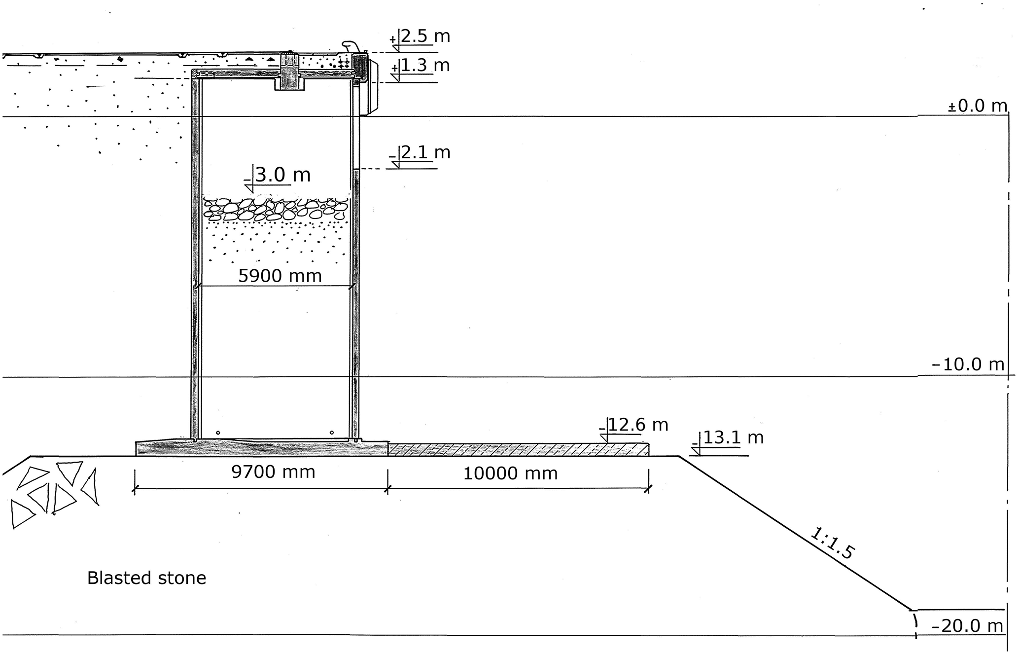
Figure 5The shoreline near the Jätkäsaari wave buoy. A part of the shoreline is equipped with wave-damping chambers. Reprinted from Björkqvist et al. (2017c).
4.3.2 Theoretical distributions
One traditional distribution used to describe the significant wave height at a certain location is the Weibull distribution (Battjes, 1972). Nevertheless, the wave conditions at the study locations in this paper are heavily influenced by e.g. the bottom topography and the numerous islands, which is why their distributions deviate from the Weibull distribution. In order to generalise the presentation of the method, we will also combine the sea level data to a set of Weibull two-parameter distributions.
These distributions have different properties: shape, expected value and typical magnitude relative to the sea level variations, with probability functions (PDFs and CDFs)
where k is the shape parameter and λ is the scale parameter. We formed three distribution pairs, each having equal scale parameter and expected value but different shape parameters (Table 1). These pairs represent three different wave conditions when compared to the still-water-level distribution (Fig. 7). The first pair (W1a and W1b) represents a typical sheltered situation where the wave height is small in comparison to the more dominant sea level variations. For the second pair (W2a and W2b) the waves and the sea level variations are of similar magnitude, while the third pair (W3a and W3b) represents waves that are clearly dominant compared to the sea level variations. The effect of the slightly larger shape parameter of distributions W1b, W2b and W3b compared to W1a, W2a and W3a can be seen as a slightly narrower and sharper form of the wave height distributions.
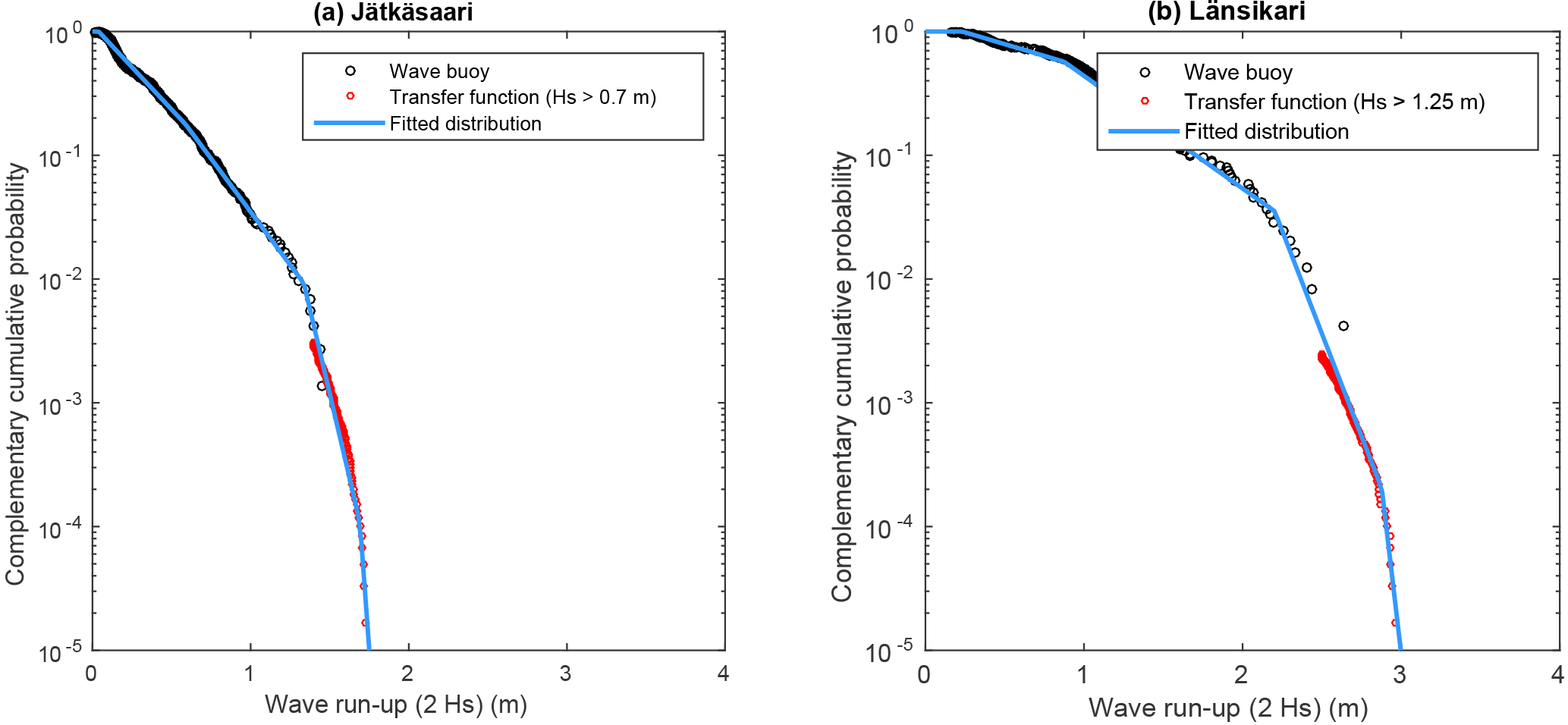
Figure 6Wave run-up distributions for the two locations in the Helsinki archipelago: Jätkäsaari and Länsikari.
Table 1The different theoretical wave run-up distributions and observation-based still-water-level distribution used for the theoretical test. The Weibull scale parameter (λ); shape parameter (k); expected value 𝔼; and 90th, 95th and 99th percentiles are given for the wave run-up distributions, and the same percentile values for the still-water-level distribution.
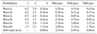
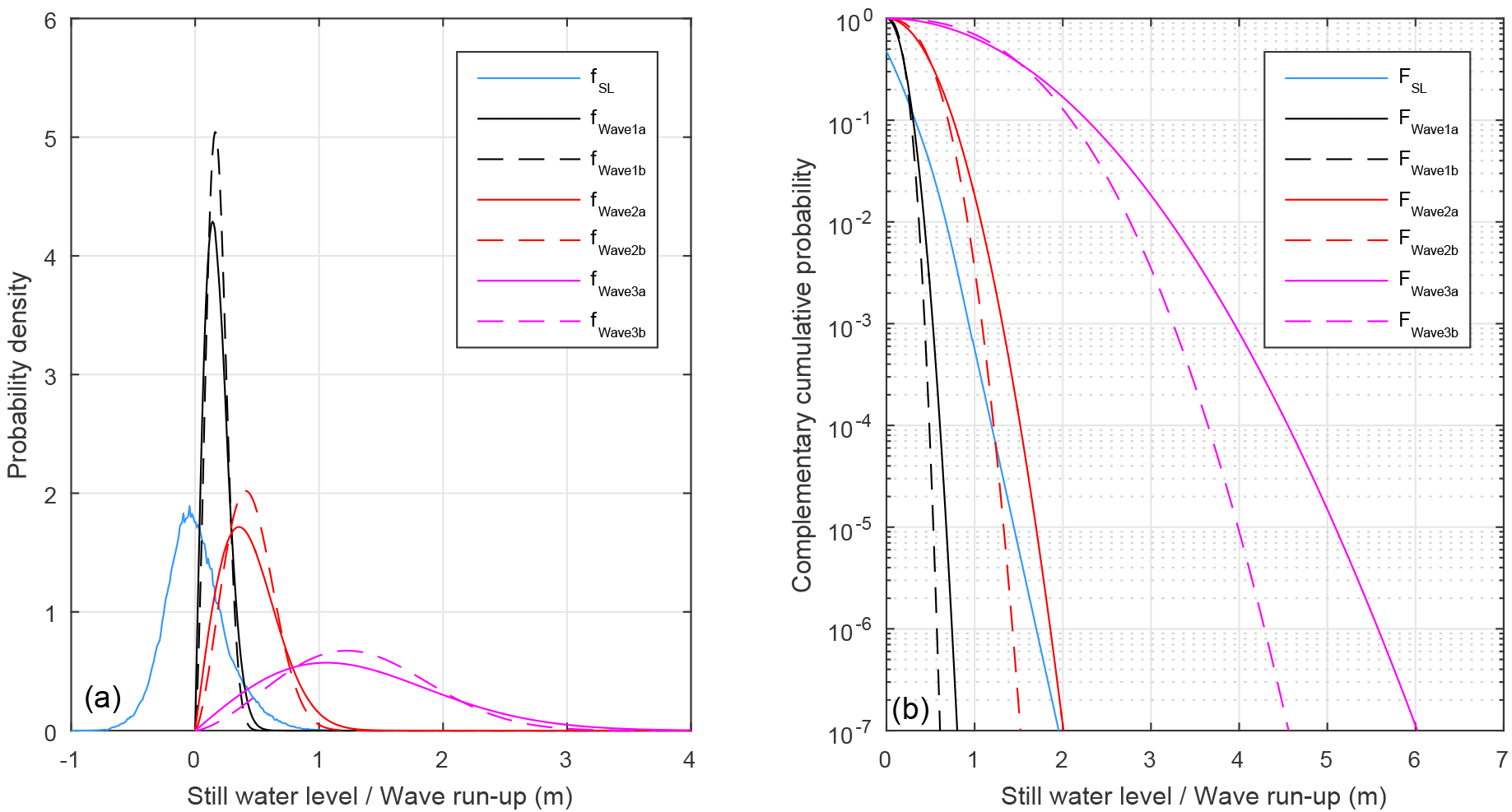
Figure 7PDFs (a) and CCDFs (b) for the still water level and the six theoretical wave run-up distributions.
4.4 Probability of the sum of two independent random variables
The theory for determining the probability distribution of the sum of two random variables can be found in textbooks (e.g. Schay, 2016), but it will nonetheless be outlined below for completeness and to introduce notation.
Let be continuous random variables, which can take values denoted by x, y and z respectively. We use the established notation of and for the associated probability density functions and cumulative distribution functions (Eq. 5). We now define to be the sum of the independent random variables and , while imposing no further constraints on or .
The goal is to define the cumulative distribution function Fz, namely expressing the probability for an arbitrary z∈ℝ. As is given as the sum , it is easy to realise that when and for any ξ∈ℝ. Consequently, when and , since . When the assumption of independence is made, the probability of the occurrence can be expressed as a product, thus yielding
Since this holds for any ξ∈ℝ and the probability is a sum of all these occurrences, we can express Fz(z) as the convolutions integral
For practical purposes fx and Fy are usually given as discrete functions. By defining the discrete functions as
for some Δξ∈ℝ and redefining fx as the probability mass function fulfilling , we end up with the discrete version of Eq. (8):
4.5 Distributions of the sum of sea level variations and wind waves
We applied the method for calculating the probability of the sum of two random variables (Sect. 4.4) to get the probability distribution of the sum of the three factors (Eq. 1) from the probability distributions of each of those (Sect. 4.1, 4.2 and 4.3). As the first step, we calculated the CDF of the still water level FSL, which accounts for the sea level variations only (SL+SS).
For the present conditions (year 2017), we calculated FSL simply by adding the long-term mean sea level estimate of 0.19 m (in the N2000 height system) to the distribution of the short-term sea level variability. For the future (years 2050 and 2100), we calculated the convolution of the PDF of the long-term mean sea level scenarios (SL) and the CDF of the short-term sea level variability (SS).
Finally, we calculated a still-water-level distribution to be used in the theoretical test by simply taking the distribution of the short-term sea level variability (SS) as such. This resulted in a distribution where the variability equals present-day short-term variability, but the mean (or expected value) is zero.
As a second step, we calculated the CDF of the full three-component sum (Eq. 1). When the notations from Sect. 4.4 are used, is the still water level SL+SS, is the run-up Hrunup and is the total water level H. Since the method is symmetric, the choice of and is in theory arbitrary. In practice, more data are required to get a good estimate of the PDF fx, which guides the proper choice of variables. We had significantly more sea level data available and will for the remainder of this paper adopt the notation fSL (“sea level”) and FW (“wave”) for fx and Fy in Eq. (9). The distribution of the total water level obtained using convolution and corresponding to Fz in Eq. (9) will be denoted .
This calculation of the three-component sum was performed for the still-water-level distributions for 2017, 2050 and 2100 combined with the observation-based wave run-up distributions at Jätkäsaari and Länsikari, as well as for the zero-mean still-water-level distribution combined with the six theoretical wave run-up distributions.
5.1 Case study in Helsinki archipelago
We applied the presented method in the Helsinki archipelago, located at the northern coast of the Gulf of Finland in the Baltic Sea. The calculations were done for two locations, where Jätkäsaari is situated deep inside the archipelago near the shoreline, while Länsikari is more exposed to the open-sea wave conditions (Fig. 2).
We calculated FSL for the still water level as a sum of two components: the short- and long-term sea level variations. Still water levels corresponding to certain frequencies of exceedance are shown in Table 2. In the convolutions FSL,W, the wave run-up was additionally accounted for, as they were calculated as a sum of three components as outlined in Sect. 4. We calculated the distributions both for the present conditions (2017) and for the future scenarios in 2050 and 2100 (Fig. 8). The total water levels representing the maximum elevation of the continuous water mass on a steep shore with selected frequencies of exceedance are given in Table 3.
The total water levels for a location closer to the open sea (Länsikari) are up to 1.2 m higher compared to the values for the sheltered shore location (Jätkäsaari). This clear difference follows from the difference in the wave run-up distributions (see Fig. 6) and highlights the variability of the waves due to locational differences, even in a rather small coastal area under investigation.
The impact of the future mean sea level change is evident in the FSL distributions for the three different years (Fig. 8). The still water levels corresponding to certain frequencies of exceedance change only slightly from 2017 to 2050 but increase significantly more from 2050 to 2100. From 2050 to 2100, the 1∕1 events year−1 still water level increases by 0.84 m, and the 1∕250 events year−1 still water level by 0.96 m (Table 2). This change results from the projected accelerating mean sea level rise in the Gulf of Finland, as well as from the wider uncertainty range in the mean sea level projections for 2100, which is reflected in the mean sea level probability distribution (for details, see Pellikka et al., 2018).
As we used the same mean sea level scenario for both Jätkäsaari and Länsikari, the effect of the mean sea level change is similar for them even in the FSL,W distributions. For example, the total water levels exceeded by 1∕100 events year−1 increase by 0.86 m in Jätkäsaari and 0.83 m in Länsikari from 2050 to 2100. The small difference between the two study locations results from the slightly different shape of the wave run-up distributions.
Table 2Still water levels (in metres relative to N2000) corresponding to certain frequencies of exceedance for three years (2017, 2050 and 2100) based on the observed sea level variability and mean sea level scenarios for the Helsinki tide gauge.
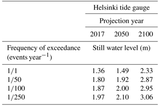
Table 3Total water levels (metres relative to N2000), as the sum of still water level and wave run-up, for three different years (2017, 2050 and 2100) for Jätkäsaari and Länsikari.
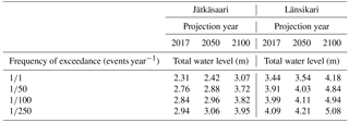
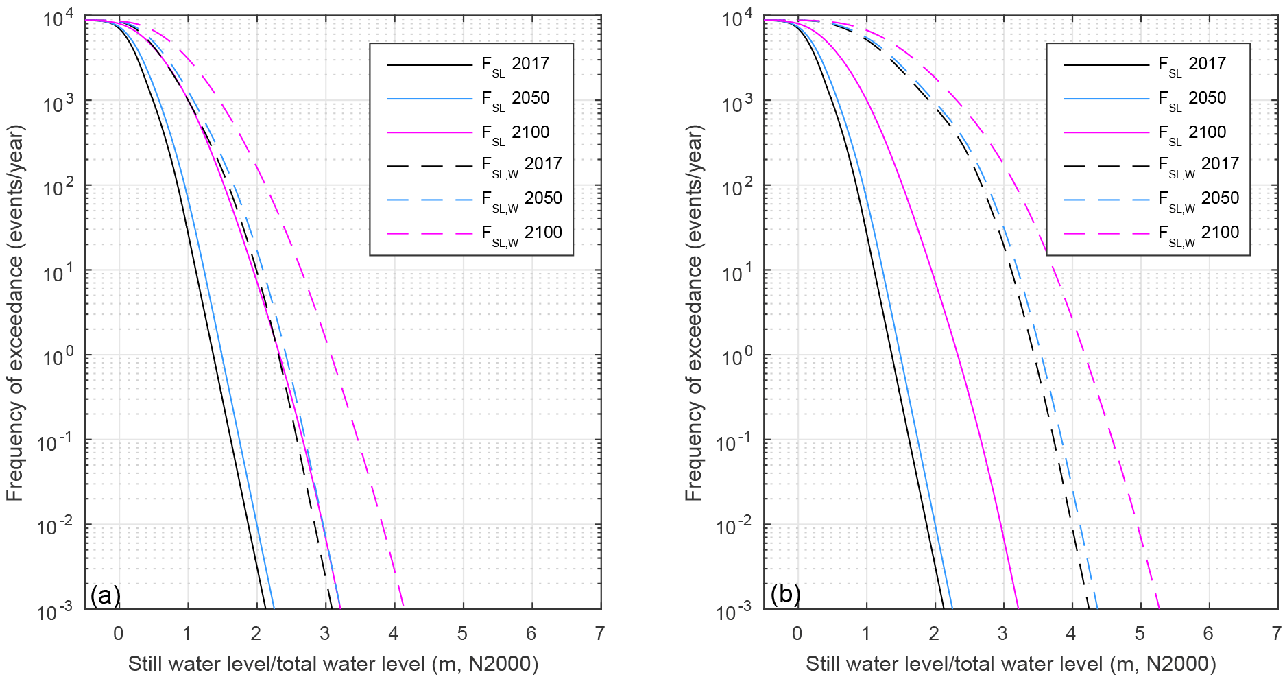
Figure 8CCDFs for the still water level alone (FSL) and the sum of the still water level and wave run-up (FSL,W) for three different years (2017, 2050 and 2100) at the two case study locations: Jätkäsaari (a) and Länsikari (b).
5.2 Test with theoretical wave run-up distributions
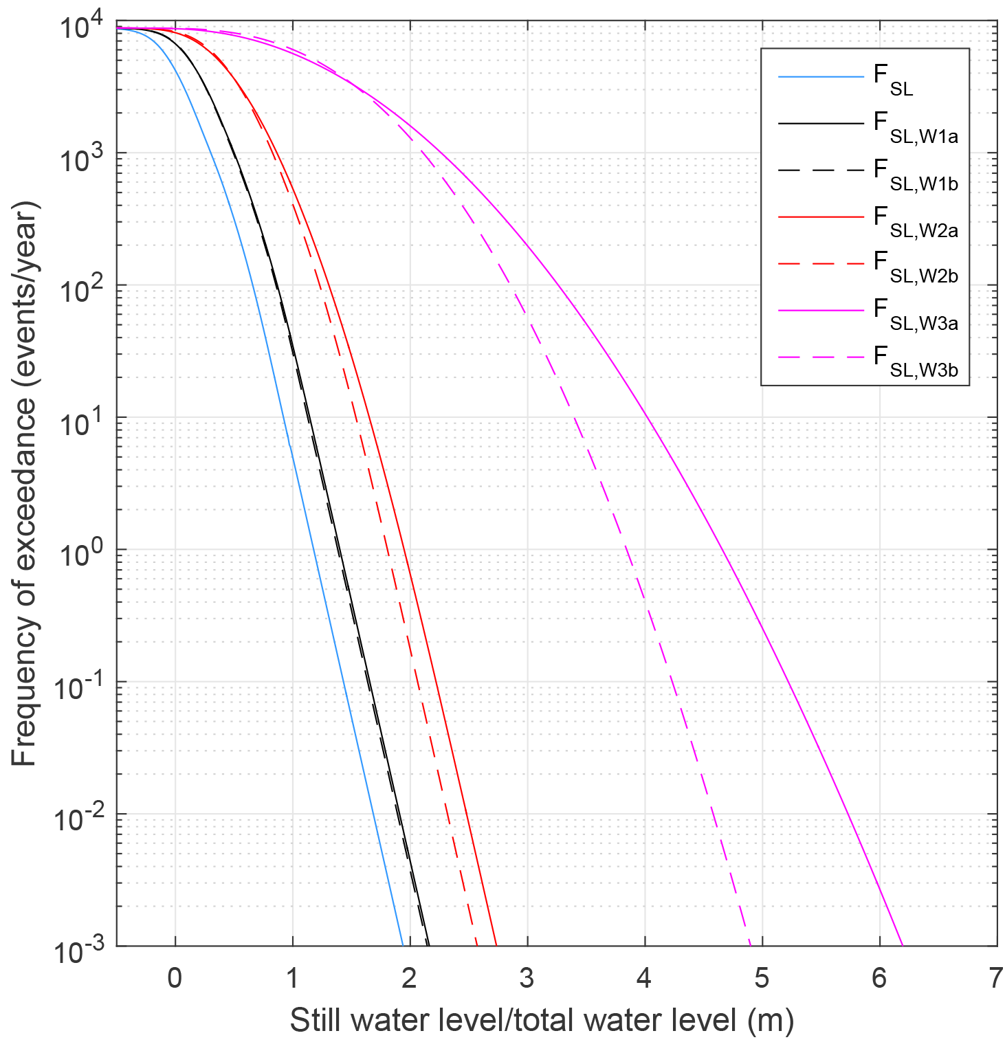
Figure 9CCDFs for the still water level and the total water level, obtained by applying six theoretical wave run-up distributions.
Table 4Results of the theoretical test, i.e. values for different frequencies of exceedance for the still-water-level distribution SL, the six theoretical wave run-up distributions W1a–W3b and the total water level distributions SL,W1a (the convolution fSL∗FW1a). The total water levels resulting from the sum of still water level and expected value of the wave run-up distributions are marked by SL + 𝔼 (W1a).
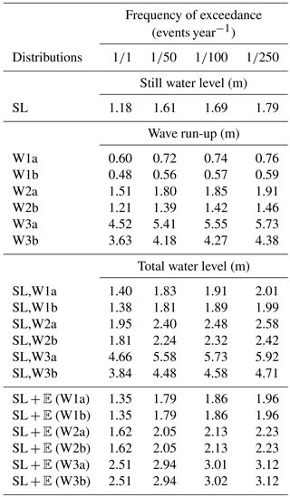
The total water level distributions SL,W1a, SL,W1b etc. obtained by combining the distribution of the short-term still water level with the theoretical wave run-up distributions, are shown in Fig. 9. We chose four different frequencies of exceedance (1∕1, 1∕50, 1∕100 and 1∕250 events year−1) for a closer examination. Table 4 summarises these for the still-water-level distribution and the six wave run-up distributions, as well as for the sum of these, i.e. the total water level distributions. As a comparison, also the corresponding still water levels added to the expected values of the wave run-up distributions are shown.
For the first pair of wave run-up distributions (W1a and W1b; see Table 1), the sea level variations clearly dominate the wave variations. The total water levels are mostly set by the still water levels; the total water levels at certain frequencies of exceedance are about 0.2 m higher than the corresponding still water levels alone. The effect of the different shapes of W1a and W1b on the results is negligible.
In the second pair (W2a and W2b), neither the wind waves nor the sea level variations are clearly dominant. The contribution of the waves is now larger compared to the first pair. Even the total water level with a frequency of 1∕1 events year−1 for the SL,W2a (1.95 m) is larger than the still water level with a frequency of 1∕250 events year−1 (1.79 m). The effect of the shapes of the wave distributions is no longer negligible. W2a has a thicker tail compared to W2b, meaning that the higher values are more probable. The difference in the total water level with a frequency of exceedance of 1∕250 events year−1 between SL,W2a and SL,W2b is 0.2 m (Table 4). This difference is caused solely by the different shapes of W2a and W2b, since they have the same expected value.
In the case of the third pair (W3a and W3b), the contribution of the larger waves becomes evident. The total water levels are up to 3.5 m (1∕1 events year−1) and 4.1 m (1∕250 events year−1) higher compared to the still water levels alone. The still water levels increase by 0.6 m from the frequency of 1∕1 events year−1 to 1∕250 events year−1, but the increase in the corresponding total water levels is 0.9–1.3 m (Table 4). Unlike in the other cases, the effect of the shape factor of the wave distribution on the total water level increases with decreasing frequencies of exceedance, being 1.2 m for 1∕250 events year−1. This shape-related behaviour is evident in Fig. 9.
With the first pair, the total water levels (SL,W1a and SL,W1b) differed by at most 0.1 m from the sum of the still water levels and expected values of the wave run-up distributions, namely SL + 𝔼 (W1a) and SL + 𝔼 (W1b). Thus, in this situation where the sea level variations dominate, simply adding the expected value of the wave run-up distribution on top of the still water levels produces results quite similar to those based on the distribution of the sum. The effect of waves on the total water level reduces to a “fixed wave action height”, which can be approximated with the expected value of the wave run-up distribution. In such cases, there is no need to calculate the distribution of the sum to obtain a good approximation of the distribution.
However, as soon as the contribution of the waves increases, the situation changes. In the situation where the wave height and sea level variations are of the same order (SL,W2a and SL,W2b vs. SL + 𝔼 (W2a) and SL + 𝔼 (W2b)), simply adding the expected value of the wave run-up distribution on top of the still water levels would underestimate the total water levels by up to 0.4 m compared to the distribution of the sum. However, when looking at the difference between the still water levels and the total water levels, we notice that the effect of the waves can still be quantified almost as a constant value to be added on top of the still water levels, “fixed wave action height”, for all the four frequencies of exceedance under inspection. However, the distribution of the sum still needs to be calculated to obtain this value, as it exceeds the expected value.
Finally, in the case where the waves dominate (SL,W3a and SL,W3b vs. SL + 𝔼 (W3a) and SL + 𝔼 (W3b)) there are large differences (up to 2.8 m), showing that the simplified solution of adding the expected value of the wave run-up distribution on top of the still water levels would lead to a remarkable underestimation of the total water level. Moreover, it is clear that in this situation the effect of the waves cannot be quantified as a constant value to be added on top of the still water levels.
5.3 Comparison of the theoretical test with the case study results
The observed wave run-up distribution at Jätkäsaari (Fig. 6) is closest to the second pair (W2a, W2b) of the theoretical distributions (Fig. 7), while the distribution at Länsikari falls between the second and third (W3a, W3b) pairs of the theoretical distributions. At both locations, the contribution of waves to the total water levels in 2017 can be quantified with a virtually constant addition to the distribution of the still water levels: 0.95–0.97 m in the case of Jätkäsaari and 2.08–2.12 m for Länsikari. Even Länsikari, where the wave variations somewhat dominate the sea level variability, does not show the behaviour characteristic for the third theoretical pair: the increase of the effect of waves with decreasing frequency of exceedance.
The same applies for the distributions of the total water level in 2050: the effect of waves adds 0.93–0.96 m to the still-water-level distribution at Jätkäsaari and 2.05–2.11 m at Länsikari. The distributions for 2100, however, behave differently. For them, the contribution of waves increases with decreasing frequency of exceedance: from 0.74 to 0.89 m at Jätkäsaari and from 1.85 to 2.02 m at Länsikari. It is also noteworthy that the contribution of waves is smaller in 2100 than in 2017 or 2050.
The effect of waves on the distributions of the total water level at Jätkäsaari and Länsikari in 2017 and 2050 can thus be quantified with a fixed wave action height, but – similar to the theoretical distributions SL,W2a and SL,W2b – this value clearly exceeds the expected value of the wave run-up distribution.
6.1 Conditions and applicability of the method
In general case, the relationships between the wave height, wave run-up and sea level variations are complex. In this study, we made several assumptions and simplifications. The aim of this section is to discuss the validity of our results, as well as to help the reader to estimate whether this method could be used at a certain location or with specific data available.
The essential prerequisites for applying the method presented above are as follows:
-
An estimate for the long-term mean sea level is needed. In its simplest form, this can be a single mean sea level height value. If the mean sea level is changing, however, an estimate for this change is needed. Again, a simple estimate could be a time-dependent mean sea level value – a linear trend, for instance. Using an ensemble of estimates for the future scenarios (like was done by Pellikka et al., 2018), however, leads to a time-dependent probability distribution for the mean sea level. Such distribution contains more information on the different possible future pathways.
-
An estimate for the range of the short-term sea level variability is needed – technically, in the form of a good-quality probability density function. In the case of the Finnish coast, we have found that several decades of observations with hourly time resolution are needed to get a reliable estimate for the extent of the local sea level variations. Additionally, to estimate total water levels with low frequencies of exceedance, such as 1∕250 events year−1 used in this study, the observation-based probability distribution – rarely extending down to frequencies below 1∕100 events year−1 – needs to be extrapolated using suitable extreme-value analysis methods.
-
An estimate for the wave run-up distribution is needed to account for the effect of waves on the coast. In this paper we have used the simplest formula for a steep shore using the highest single wave, which was estimated from the significant wave height Hs. The method can be generalised by using wave run-up formulations that also account for e.g. the slope of the beach.
-
We based our analysis on a simplifying assumption that the sea level variations and wave run-up are independent. This makes it possible to calculate the distribution of the sum from the marginal distributions without additional assumptions. In practice, the independence of the variables can be, at least partly, achieved for locations with a constant beach profile, such as deep and steep shores. Strong wind-independent components in the sea level also decrease the dependence of the sea level and the wave run-up. In the Baltic Sea, such a component is the total Baltic Sea water volume, which, although expressing a strong correlation with the wind conditions (Johansson et al., 2014), does so on a timescale much longer than that of the wind waves. In addition, the mutual dependence of the sea level and waves is weakened in the Gulf of Finland, since strong easterly winds lower the sea level by emptying the gulf. Tidal variations are also a sea level component which is independent of waves; such variations are small on the Finnish coast, however.
As long as the above conditions are met, we consider the method presented here applicable also for other places than the Finnish coast. Naturally, as the most important factors causing sea level variations are different in different places, this needs to be taken into account. For instance, in places where the tidal variations dominate over storm surges, a different analysis of the short-term sea level variability might be appropriate.
6.2 Limitations and potential improvements
In our approach, we treated the still-water-level variations and the wave run-up as independent variables as a first approximation. The limited amount of wave data available for this study imposed challenges in the construction of the full joint distribution, which would have taken into account the possible dependencies between these variables. The dependency might be affected by the location-specific circumstances, and further studies are needed to determine the conditions under which the use of the full two-dimensional distributions is preferable to assuming independence.
Pellikka et al. (2018) used the observed monthly maxima of sea levels on the Finnish coast to calculate the location-specific short-term sea level variability distributions. They calculated the probability distribution of the sum of long- and short-term sea level variations with a method similar to the one we used to calculate the FSL distribution. By this method they analysed the present and future flooding risks on the Finnish coast. Our results for still water levels with frequencies of exceedance of 1∕1, 1∕50 and 1∕100 events year−1 (Table 2) are higher than those of Pellikka et al. (2018). This is likely explained by the differences in statistics. Several high hourly sea level values can occur during the same month, or even the same storm surge event, and still result in only one monthly maximum in the statistics. Thus, the hourly values have a higher frequency of exceedance than the monthly maxima, reflecting the difference in the definition of “an event” in each case.
Using block maxima of sea level variations – such as the monthly maxima used by Pellikka et al. (2018) – in our analysis would implicitly restrict the study of the joint effect to cases where the still water level is high, thus excluding combinations of moderate still water level and high waves.
We calculated the future scenarios for the flooding risks by simply combining the mean sea level scenarios with the present-day short-term sea level variability and wave conditions. Thus, we implicitly assumed that those will not change in the future. A potential improvement, to get deeper insight into the changes of flooding risks in the future, would be to include scenarios of short-term sea level variability or wave conditions. As these both mainly depend on short-term weather (wind and air pressure) conditions, this would require scenarios for the short-term weather variability.
Safe coastal building elevations are usually estimated for structures with a designed lifetime of at least several decades, but the relevant safety margins differ between commercial buildings, residential buildings and e.g. nuclear power plant sites. We therefore need to consider scenarios up to 2100 and frequencies of exceedance as rare as 1∕250 events year−1 or even less. The approach presented in this paper allows for the determining of different building levels based on the acceptable risks for various infrastructure, thus reducing building costs while maintaining necessary safety margins. Thereby it assists in a cost-effective coastal planning to meet the requirements of the changing climate of the future.
In this study, a location-specific statistical method was used for the first time on the Finnish coast to evaluate flooding risks based on the joint effect of three components: (1) long-term mean sea level change, (2) short-term sea level variability and (3) wind-generated waves. We conducted an observation-based case study for two locations with steep shorelines and performed a test with theoretical wave run-up distributions.
The case study at the Helsinki archipelago (Sect. 5) showed that the flooding risk estimates are sensitive to local wave conditions: the total water levels at the site close the open sea (Länsikari) were clearly higher compared to the values at the sheltered location near the shoreline (Jätkäsaari). This finding highlights the need for a location-specific evaluation of the wave height to prevent over- or underestimation of the joint effect, especially in places with an irregular coastline.
We found the coastal flooding risks at our case study location to increase towards the end of the century. This behaviour in our results is due to the projected mean sea level rise as well as increasing uncertainties in these projections (Pellikka et al., 2018). It is noteworthy that the frequencies of exceedance given for certain total water levels in our distributions for 2100 do not represent the actual flooding risk in that year. Instead, they are statistical estimates, which include the uncertainty due to the range of possible mean sea level scenarios. Eventually, only one (or none) of these scenarios will be realised in 2100.
Our test with the theoretical wave run-up distributions showed that, in a situation where the sea level variations dominate over waves, simply adding the expected value of the wave run-up on top of the still-water-level distribution produces results close to the distribution of the sum. However, when the contribution of the waves increases, such addition leads to an underestimation of the effect of waves on the total water levels. Finally, when the waves are clearly dominant, their effect starts to depend on the frequency of exceedance and cannot be quantified as a constant value to be added on top of the still water levels anymore.
Please see the Supplement for our data.
The supplement related to this article is available online at: https://doi.org/10.5194/nhess-18-2785-2018-supplement.
The research question was proposed by KK. Sea level data were analysed by UL and MJ, and wind wave data by JVB and KK. The mean sea level scenarios were prepared by HP. KK, MJ and UL combined the probability distributions of sea level variations and wave run-up. The compiling of the manuscript was initiated by UL and LL, and it was mainly written by UL, JVB and MJ with contributions from all co-authors.
The authors declare that they have no conflict of interest.
This research was partly funded by the Finnish State Nuclear Waste
Management Fund (VYR) through SAFIR2018 (the Finnish Research Programme on
Nuclear Power Plant Safety 2015–2018), the City of Helsinki, and Arvid och
Greta Olins fond (Svenska kulturfonden, 15/0334-1505). This study has utilised
research infrastructure facilities provided by FINMARI (Finnish Marine Research
Infrastructure network). We would like to thank the three referees for constructive
comments, which helped us to improve the manuscript.
Edited by: Piero Lionello
Reviewed by: Jose A. Jiménez and two anonymous referees
Battjes, J. A.: Long-term wave height distributions at seven stations around the British Isles, Deutsche Hydrographische Zeitschrift, 25, 179–189, https://doi.org/10.1007/BF02312702, 1972. a
Björkqvist, J.-V., Tuomi, L., Fortelius, C., Pettersson, H., Tikka, K., and Kahma, K. K.: Improved estimates of nearshore wave conditions in the Gulf of Finland, J. Mar Syst., 171, 43–53, https://doi.org/10.1016/j.jmarsys.2016.07.005, 2017a. a, b
Björkqvist, J.-V., Tuomi, L., Tollman, N., Kangas, A., Pettersson, H., Marjamaa, R., Jokinen, H., and Fortelius, C.: Brief communication: Characteristic properties of extreme wave events observed in the northern Baltic Proper, Baltic Sea, Nat. Hazards Earth Syst. Sci., 17, 1653–1658, https://doi.org/10.5194/nhess-17-1653-2017, 2017b. a
Björkqvist, J.-V., Vähäaho, I., and Kahma, K.: Spectral field measurements of wave reflection at a steep shore with wave damping chambers, WIT Trans. Built Env., 170, 185–191, 2017c. a, b, c, d
Cannaby, H., Palmer, M. D., Howard, T., Bricheno, L., Calvert, D., Krijnen, J., Wood, R., Tinker, J., Bunney, C., Harle, J., Saulter, A., O'Neill, C., Bellingham, C., and Lowe, J.: Projected sea level rise and changes in extreme storm surge and wave events during the 21st century in the region of Singapore, Ocean Sci., 12, 613–632, https://doi.org/10.5194/os-12-613-2016, 2016. a
Cheon, S.-H. and Suh, K.-D.: Effect of sea level rise on nearshore significant waves and coastal structures, Ocean Eng., 114, 280–289, 2016. a
Chini, N. and Stansby, P.: Extreme values of coastal wave overtopping accounting for climate change and sea level rise, Coast. Eng., 65, 27–37, 2012. a
Chini, N., Stansby, P., Leake, J., Wolf, J., Roberts-Jones, J., and Lowe, J.: The impact of sea level rise and climate change on inshore wave climate: A case study for East Anglia (UK), Coast. Eng., 57, 973–984, 2010. a
Hanson, H. and Larson, M.: Implications of extreme waves and water levels in the southern Baltic Sea, J. Hydraulic Res., 46, 292–302, 2008. a
Hawkes, P.: Joint probability analysis for estimation of extremes, J. Hydraulic Res., 46, 246–256, 2008. a
Hawkes, P., Gouldby, B., Tawn, J., and Owen, M.: The joint probability of waves and water levels in coastal engineering design, J. Hydraulic Res., 40, 241–251, 2002. a
Johansson, M. M., Boman, H., Kahma, K. K., and Launiainen, J.: Trends in sea level variability in the Baltic Sea, J. Mar. Syst., 6, 159–179, 2001. a, b
Johansson, M. M., Pellikka, H., Kahma, K. K., and Ruosteenoja, K.: Global sea level rise scenarios adapted to the Finnish coast, J. Mar. Syst., 129, 35–46, https://doi.org/10.1016/j.jmarsys.2012.08.007, 2014. a, b, c, d, e
Kahma, K., Pettersson, H., Boman, H., and Seinä, A.: Alimmat suositeltavat rakennuskorkeudet Pohjanlahden, Saaristomeren ja Suomenlahden rannikoilla, 1998 (in Finnish). a
Kahma, K., Pellikka, H., Leinonen, K., Leijala, U., and Johansson, M.: Pitkän aikavälin tulvariskit ja alimmat suositeltavat rakentamiskorkeudet Suomen rannikolla (Long-term flooding risks and recommendations for minimum building elevations on the Finnish coast), available at: http://hdl.handle.net/10138/135226 (last access: 17 October 2018), 2014 (in Finnish with English summary). a
Kahma, K. K. and Pettersson, H.: Wave growth in narrow fetch geometry, The Global Atmosphere and Ocean System, 2, 253–263, 1994. a
Kahma, K. K., Björkqvist, J.-V., Johansson, M., Jokinen, H., Leijala, U., Särkkä, J., Tikka, K., and Tuomi, L.: Turvalliset rakentamiskorkeudet Helsingin rannoilla 2020, 2050 ja 2100 (Safe building elevations on the Helsinki coast in 2020, 2050 and 2100), available at: http://www.hel.fi/static/kv/turvalliset-rakentamiskorkeudet.pdf (last access: 17 October 2018), 2016 (in Finnish with English abstract). a, b, c, d
Leppäranta, M. and Myrberg, K.: Physical Oceanography of the Baltic Sea, Springer, 2009. a, b, c
Longuet-Higgins, M.: On the Statistical Distribution of the Heights of Sea Waves, J. Mar. Res., 11, 245–266, 1952. a
Masina, M., Lamberti, A., and Archetti, R.: Coastal flooding: A copula based approach for estimating the joint probability of water levels and waves, Coast. Eng., 97, 37–52, 2015. a
Parjanne, A. and Huokuna, M.: Tulviin varautuminen rakentamisessa – opas alimpien rakentamiskorkeuksien määrittämiseksi ranta-alueilla (Flood preparedness in building – guide for determining the lowest building elevations in shore areas), http://hdl.handle.net/10138/135189 (last access: 17 October 2018), 2014 (in Finnish with English summary). a
Pellikka, H., Rauhala, J., Kahma, K., Stipa, T., Boman, H., and Kangas, A.: Recent observations of meteotsunamis on the Finnish coast, Nat. Hazards, 74, 197–215, 2014. a
Pellikka, H., Leijala, U., Kahma, K. K., Leinonen, K., and Johansson, M. M.: Future probabilities of coastal floods in Finland, Cont. Shelf Res., 157, 32–42, https://doi.org/10.1016/j.csr.2018.02.006, 2018. a, b, c, d, e, f, g, h, i, j, k, l, m
Pettersson, H., Lindow, H., and Brüning, T.: Wave climate in the Baltic Sea 2012, http://www.helcom.fi/baltic-sea-trends/environment-fact-sheets/hydrography/wave-climate-in-the-baltic-sea/ (last access: 17 October 2018), 2013. a
Pindsoo, K. and Soomere, T.: Contribution of wave set-up into to the total water level in the Tallinn area, P. Est. Acad. Sci., 64, 338–348, 2015. a
Prime, T., Brown, J. M., and Plater, A.: Flood inundation uncertainty: The case of a 0.5% annual probability flood event, Environ. Sci. Pol., 59, 1–9, 2016. a
Saaranen, V., Lehmuskoski, P., Rouhiainen, P., Takalo, M., Mäkinen, J., and Poutanen, M.: The new Finnish height reference N2000, in: Geodetic Reference Frames, edited by: Drewes, H., IAG Symposium Munich, Germany, 9–14 October 2006, Springer, 297–302, 2009. a
Särkkä, J., Kahma, K. K., Kämäräinen, M., Johansson, M. M., and Saku, S.: Simulated extreme sea levels at Helsinki, Boreal Environ. Res., 22, 299–315, 2017. a, b
Schay, G.: Introduction to Probability with Statistical Applications, Springer International Publishing, Switzerland, https://doi.org/10.1007/978-3-319-30620-9, 2016. a
Soomere, T., Pindsoo, K., Bishop, S. R., Käärd, A., and Valdmann, A.: Mapping wave set-up near a complex geometric urban coastline, Nat. Hazards Earth Syst. Sci., 13, 3049–3061, https://doi.org/10.5194/nhess-13-3049-2013, 2013. a
Suursaar, Ü., Kullas, T., Otsmann, M., Saaremäe, I., Kuik, J., and Merilain, M.: Cyclone Gudrun in January 2005 and modelling its hydrodynamic consequences in the Estonian coastal waters, Boreal Environ. Res., 11, 143–159, 2006. a
Tõnisson, H., Orviku, K., Jaagus, J., Suursaar, Ü., Kont, A., and Rivis, R.: Coastal damages on Saaremaa Island, Estonia, caused by the extreme storm and flooding on January 9, 2005, J. Coast. Res., 24, 602–614, 2008. a
Tuomi, L., Kahma, K., and Pettersson, H.: Wave hindcast statistics in the seasonally ice-covered Baltic Sea, Boreal Environ. Res., 16, 451–472, 2011. a
Tuomi, L., Pettersson, H., Fortelius, C., Tikka, K., Björkqvist, J.-V., and Kahma, K.: Wave modelling in archipelagos, Coast. Eng., 83, 205–220, 2014. a
Wahl, T., Mudersbach, C., and Jensen, J.: Assessing the hydrodynamic boundary conditions for risk analyses in coastal areas: a multivariate statistical approach based on Copula functions, Nat. Hazards Earth Syst. Sci., 12, 495–510, https://doi.org/10.5194/nhess-12-495-2012, 2012. a
Witting, R.: Tidvattnen i Östersjön och Finska Viken, Fennia, 29:2, 1911. a
- Abstract
- Introduction
- Components contributing to the sea surface level
- Scenarios and observations used in this study
- Probability methods to combine sea level variations and wind waves
- Results
- Discussion
- Conclusions
- Data availability
- Author contributions
- Competing interests
- Acknowledgements
- References
- Supplement