Implementation and validation of a new operational wave forecasting system of the Mediterranean Monitoring and Forecasting Centre in the framework of the Copernicus Marine Environment Monitoring Service

Within the framework of the Copernicus Marine Environment Monitoring Service (CMEMS), an operational wave forecasting system for the Mediterranean Sea has been implemented by the Hellenic Centre for Marine Research (HCMR) and evaluated through a series of preoperational tests and subsequently for 1 full year of simulations (2014). The system is based on the WAM model and it has been developed as a nested sequence of two computational grids to ensure that occasional remote swell propagating from the North Atlantic correctly enters the Mediterranean Sea through the Strait of Gibraltar. The Mediterranean model has a grid spacing of 1∕24^∘. It is driven with 6-hourly analysis and 5-day forecast 10 m ECMWF winds. It accounts for shoaling and refraction due to bathymetry and surface currents, which are provided in offline mode by CMEMS. Extensive statistics on the system performance have been calculated by comparing model results with in situ and satellite observations. Overall, the significant wave height is accurately simulated by the model while less accurate but reasonably good results are obtained for the mean wave period. In both cases, the model performs optimally at offshore wave buoy locations and well-exposed Mediterranean subregions. Within enclosed basins and near the coast, unresolved topography by the wind and wave models and fetch limitations cause the wave model performance to deteriorate. Model performance is better in winter when the wave conditions are well defined. On the whole, the new forecast system provides reliable forecasts. Future improvements include data assimilation and higher-resolution wind forcing.

1 Introduction

In recent years the requirements of the marine industry for real-time wave forecasts have increased substantially. Various sectors such as, for example, maritime transport, shipping, and offshore mineral industry require accurate wave forecasts in order to secure operations at sea, save fleet fuel consumption using more accurate routing, and prevent from potential ship and platform oil spill drift. In addition, a detailed wave information along coastal regions is crucial for coast guards and port authorities as there is the need to anticipate wave conditions that could interfere in ships arriving and leaving the harbours. Furthermore, wave forecasting provides significant advantages for the offshore wind and the wave energy so as to schedule installation and maintenance activities, to define control strategies according to the predominant wave conditions, or to plan for storm events. Scientifically, waves are a bridge between the ocean and the atmosphere, playing a key role in air–sea interaction and are also an important mixing agent with an active role in erosion and resuspension processes.

The dramatic increase in computing power and the enhanced understanding of the physical processes responsible for wave generation, evolution, and dissipation have resulted in third-generation wave models which use first principles in the integration of an action or energy balance equation (Tolman, 1992) based on the sophisticated physics pertaining to wave generation, propagation, and decay mechanisms. Wave models like WAM (WAMDI Group, 1988; Komen et al., 1994), WAVEWATCH III (Tolman, 1991, 1999), and SWAN (Booij et al., 1999) are being used by many meteorological and oceanographic operational centres and have been reasonably successful in operational wave predictions at the global, regional, and coastal scales. One of the pioneers in the implementation and the development of wave analysis and forecast systems is the European Centre for Medium Weather Forecasts (ECMWF), which has provided daily medium-range global wave forecasts up to 10 days ahead since 1992. With time, more centres (e.g. UK Met Office, the Service Hydrographique et Océanographique de la Marine (SHOM), and several others) began to use state-of-the-art third-generation numerical wave models in operational forecasting. In addition, an international wave forecast inter-comparison project was established (Bidlot, 2007), coordinated by the ECMWF, to evaluate forecast quality and performance and identify areas of potential improvement (Breivik et al., 2015).

The EU-funded Copernicus Marine Environmental Monitoring Service (CMEMS) driven by the requirements of a large user panel in need of wave information in all ocean basins has enriched its portfolio since early 2017 with the provision of open, cost-free, and quality-controlled wave products for the global ocean and regional European seas. CMEMS is based on a strong European partnership with more than 50 marine operational and research centres in Europe involved in marine monitoring and forecasting services and their evolution, providing a wide range of marine measurements of social and environmental value such as ocean currents, temperature, salinity, sea level, pelagic biogeochemistry, and waves. The backbone of the CMEMS relies on a Central Information System (CIS) and an architecture of production centres inherited from the MyOcean projects for both observations (Thematic Assembly Centre – TAC) and modelling–assimilation (Monitoring and Forecasting Centre – MFC). The MFCs are distributed according to the marine area covered and generate model-based products including analysis of the current situation, forecasts of the situation a few days in advance, and the provision of retrospective data records (reanalysis). Detailed information on the systems and products is on CMEMS web site: http://marine.copernicus.eu/ (last access: September 2018). The Mediterranean Sea (Med) MFC is composed of INGV (Italy), HCMR (Greece), OGS (Italy), and the Euro-Mediterranean Centre on Climate Change (CMCC, Italy). It is an expert consortium with profound expertise in the Mediterranean phenomenology and dynamics, from waves to currents, and biogeochemistry, and it provides regular and systematic information about the physical state of the ocean and the dynamics of the marine ecosystem of the basin.

In this study we present the wave component of the Med MFC, a high-resolution operational wave forecasting system (hereafter called Med-waves), which has been developed by HCMR and provides daily accurate products – wave simulations and 5-day forecasts – of the wave environment of the Mediterranean Sea to the general public through the CMEMS portal. The system employs the WAM Cycle 4.5.4 (Günther and Behrens, 2012), a modernized and improved version of the WAM model. In this study, a modelling system consisting of a nesting sequence of two computational grids (North Atlantic and Mediterranean) has been developed with the fine-grid model covering the Mediterranean Sea and the coarse-grid model the North Atlantic. A nesting approach of this kind enables us to properly simulate the effect of the remotely generated Atlantic swell into the Mediterranean Sea as it passes through the Strait of Gibraltar. In fact, Cavaleri and Sclavo (2006) pointed out that the narrow Strait of Gibraltar appreciably affects the wave climate in the close-by area of the Alboran Sea and it is often neglected in wave modelling systems of the Mediterranean Sea. Moreover, the system incorporates offline coupling with general circulation models (CMEMS global and Mediterranean analysis and forecast systems) to provide surface currents for wave refraction to both nests of the modelling system. Refraction due to surface currents impacts the wave spectrum to some extent. Its impact on improving the wave forecast is addressed by Osuna and Wolf (2005), Clementi et al. (2013, 2017), and Mao and Xia (2017). Thus, while in the last years few operational centres have already developed and implemented regional wave forecast systems for the entire Mediterranean, none of these take into account the sensitivity of Mediterranean wave dynamics to the nesting with the Atlantic, at the same time incorporating the surface currents effect on wave refraction. In addition, the system offers an extended set of freely available wave products and has a spatial and spectral resolution high enough to describe with sufficient accuracy the wind wave dynamics over the Mediterranean Basin.

Despite the diversity of wave generation models as well as of atmospheric models, obtaining good quality of short-term wave forecasts for the Mediterranean Sea is still a difficult task due to the large spatial and temporal variability in the surface wind field over the basin (e.g. Bidlot, 2017). Wind-wave models are very sensitive to wind field variations, which result in one of the main source of errors in wave predictions. The sensitivity of wave model prediction to variations in wind forcing fields has been studied by several authors (Komen et al., 1994; Teixeira et al., 1995; Holthuijsen et al., 1996; Ponce and Ocampo-Torres, 1998). This is particularly true for the Mediterranean where the limited contribution of swell to the wave spectrum makes the regional wind conditions the most important factor in determining the local wave state. Bearing in mind this context, the complex structure of the Mediterranean Sea due to the presence of large mountainous islands, protruding peninsulas, jagged coastlines, and sharp orography gradients deeply influences the wind and wave dynamics, especially close to the coast, making the local forecast particularly challenging. Many authors have highlighted the fact that forecasted winds in the Mediterranean are not as accurate as in the open ocean (Cavaleri and Bertotti, 2003, 2004; Bolaños et al., 2005; Signell et al., 2005; Ardhuin et al., 2007; Bolaños-Sanchez et al., 2007) and advocate the necessity of further improvement on the wind field quality as well as the increase in its spatial resolution, especially in enclosed basins such as the Mediterranean Sea (Cavaleri et al., 1991; Cavaleri and Bertotti, 2004, 2009a, b; Bentamy et al., 2007; Lionello et al., 2008). Today, the full coupling of different geophysical models (e.g. atmospheric, ocean, wave) is also a favoured approach to reduce the wind forecasting error, especially in dynamically complicated coastal areas, as it accounts for the complex interactions of waves, currents, and the atmosphere (Wahle et al., 2017). For the Mediterranean Sea, the added value of coupled air–sea models has been demonstrated by many research groups (Artale et al., 2009; Renault et al., 2012; Katsafados et al., 2016; Varlas et al., 2018) particularly in the region of the Adriatic Sea (Pullen et al., 2006; Carniel et al., 2016; Licer et al., 2016; Ricchi et al., 2016) where the synoptic wind regimes are difficult to forecast. However, despite the rapid progress and the encouraging results of this field, there are still open scientific issues such as missing physics and poor parameterizations for the coupled atmospheric–ocean–wave processes in the air–sea interaction zone, especially under extreme wind and ocean conditions (Chen et al., 2007; Soloviev et al., 2014). Furthermore, the coupled models are still computationally expensive and even with increased computational potential to date only few major meteorological and oceanographic centres have the capability to incorporate these high computationally demanding systems at fine spatiotemporal resolution and at large spatial scales into their operational weather–ocean forecasting chains. The recent white paper by Cavaleri et al. (2018) analyses in detail the various aspects and problems affecting the performance of wave models in enclosed and inner seas including the Mediterranean Sea. In this framework, the selection of an appropriate wind forcing is a vital step in the operational wave modelling of the Mediterranean Sea. As such, the Med-waves system in particular uses the analysis and forecast wind fields produced by the ECMWF Integrated Forecasting System (IFS). The quality and appropriateness of ECMWF 10 m winds for wave simulations and forecasting in different areas has been demonstrated by many studies. On a global scale, repetitive statistics have shown that the ECMWF products are, and have been for a long while, the best ones in the world (Bertotti et al., 2011). However, for semi-enclosed basins, the quality of ECMWF wind fields decreases and the wave model underestimates the high wave heights because of the underestimation of high wind speeds (Cavaleri and Bertotti, 2004; Signell et al., 2005; Cavaleri and Scalvo, 2006; Saket et al., 2013) and/or overestimates the lower ones because of the overestimation of low wind speeds by ECMWF (Moeini et al., 2010). In our system, this underestimation of wind is compensated for by reducing the energy loss due to whitecapping, performing a fine tuning of the free parameters of the dissipation function.

We present here the first comprehensive documentation of the system and the evaluation of its accuracy over a period of 1 year (2014). The rest of the paper is organized as follows. A detailed description of the Med-waves modelling system is given in Sect. 2. Section 3 outlines the methodology followed in the model validation, and Sect. 4 is devoted to the validation results including both hindcast and forecast skill evaluation against in situ and satellite observations. Finally, a summary and some concluding remarks are given in Sect. 5.

2 The wave forecasting system

As previously stated, Med-waves is based on the WAM Cycle 4.5.4 wave model, a state-of-the-art third-generation wave model which is a modernized and improved version of the well-known and extensively used WAM Cycle 4 wave model (WAMDI Group, 1988; Komen et al., 1994). Cycle 4.5.4 has been released during the MyWave (“A pan-European concerted and integrated approach to operational wave modelling and forecasting – a complement to GMES MyOcean services”) EU FP7 research project and is freely available to the entire research and forecasting community. WAM solves the wave transport equation explicitly without any presumption on the shape of the wave spectrum. Its source–sink terms include the wind input, whitecapping dissipation, non-linear transfer, and bottom friction. The wind input and whitecapping dissipation source terms of the present cycle of the wave model are a further development based on Janssen's quasilinear theory of wind-wave generation (Janssen, 1989, 1991). The non-linear transfer term is a parameterization of the exact non-linear interactions as proposed by Hasselmann and Hasselmann (1985) and Hasselmann et al. (1985). Lastly, the bottom friction term is based on the empirical JONSWAP model of Hasselmann et al. (1973).

The Med-waves set-up includes a coarse-grid domain with a resolution of 1∕6^∘ covering the North Atlantic Ocean (NA) from 75^∘ W to 10^∘ E and from 10 to 70^∘ N and a nested fine-grid domain with a resolution of 1∕24^∘ covering the Mediterranean Sea from 18.125^∘ W to 36.2917^∘ E and from 30.1875 to 45.9792^∘ N. The areas covered by the two grids are shown in Fig. 1, which is a schematic of the Med-waves system. The bathymetric map has been constructed using the GEBCO 30 s bathymetric data set (GEBCO, 2016) for the Mediterranean Sea model and the ETOPO2 2 min bathymetric data set (NGDC, 2006) for the North Atlantic model.

Figure 1 Schematic of the Med-waves system.

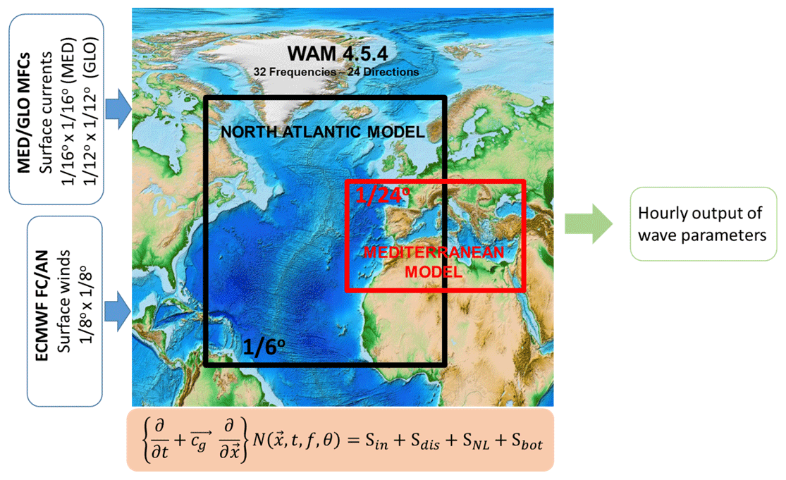
The Mediterranean Sea model receive the full wave spectrum at hourly intervals at its Atlantic Ocean open boundary from the North Atlantic model. The latter model is considered to have all of its four boundaries closed with no wave energy propagation from the adjacent seas. Because of the wide geographical coverage of the North Atlantic model, the consideration of closed boundaries does not affect the swell propagation towards the open boundary of the Mediterranean model, which is the main interest of this nesting approach.

The wave spectrum is discretized using 32 frequencies, which cover a logarithmically scaled frequency band from 0.04177 to 0.8018 Hz at intervals of $\frac{df}{f}=\mathrm{0.1}$ and 24 equally spaced directions (15^∘ bin size).

The Mediterranean model runs in shallow-water mode considering wave refraction due to depth and currents in addition to depth-induced wave breaking. The North Atlantic model runs in deep-water mode with wave refraction due to currents only. The North Atlantic model additionally considers wave energy damping due to the presence of sea ice.

Following ECMWF (2015), the tunable whitecapping dissipation coefficients C_dis and δ have been altered from their default values. Specifically, the values of C_dis=1.33 (C_dis=2.1 default) and δ=0.5 (δ=0.6 default) have been adopted. The aim of this tuning is to produce results which are in good agreement with data on fetch-limited growth and with data on the dependence of the surface stress on wave age.

The atmospheric forcing of the Med-waves system is the operational 10 m wind analysis and forecast from the ECMWF global meteorological forecasting system (ECMWF, 2017) that are disseminated at a horizontal resolution of 1∕8^∘. The quality of the ECMWF forecasts is regularly evaluated (Haiden et al., 2016). Sea ice coverage fields are also obtained from ECMWF IFS at the same horizontal resolution as the wind fields. An issue here concerns the temporal resolution of the disseminated ECMWF wind fields as these data are provided on a 3-hourly basis for the first 3 days of the forecast while it is expected that higher-temporal-resolution wind forcing can better capture storm events, especially if the latter have a short duration. For example, Alomar et al. (2014) have shown that on the southern Catalan coast (NW Mediterranean Sea), the best wind speed estimations, compared with the observations, corresponded to a grid size of 4 km and a temporal resolution of 1 h.

Surface current forcing is accounted for in Med-waves. The Mediterranean Sea model is forced by surface currents obtained from the physical forecasting system of the CMEMS Med-MFC at 1∕16^∘ horizontal resolution (CMEMS, 2016a) and the North Atlantic model by surface currents obtained from the physical forecasting system of the CMEMS Global-MFC at 1∕12^∘ horizontal resolution (CMEMS, 2016b). Both physical forecasting systems are based on the Nucleus for European Modelling of the Ocean (NEMO) ocean physics model, which is a state-of-the-art free-surface primitive equation model (Madec, 2008). NEMO is free software used by a large community.

Med-waves is run once per day starting at 12:00:00 UTC. It produces 5-day forecast fields initialized by a 1-day hindcast. The wave hindcast is forced by 6-hourly analysis wind fields and daily averaged analysis current fields. The 5-day forecast is forced by 3-hourly forecast wind fields for the first 3 days and 6-hourly forecast wind fields for the rest of the forecast cycle. Daily averaged forecast currents are used over the entire wave forecast. Sea ice coverage fields are updated at daily frequency and remain constant during the forecast cycle.

Figure 2 Wave buoys' location and unique ID code.

Med-waves generates hourly wave fields over the Mediterranean Sea at 1∕24^∘ horizontal resolution. These wave fields correspond either to wave parameters computed by integration of the total wave spectrum or to wave parameters computed using wave spectrum partitioning. In the latter case the complex wave spectrum is partitioned into wind sea and primary and secondary swell. Wind sea is defined as those wave components that are subject to wind forcing while the remaining part of the spectrum is termed swell. Wave components are considered to be subject to wind forcing when

$$\begin{array}{}\text{(1)}& {\displaystyle }{\displaystyle }c\le \mathrm{1.2}\times \mathrm{28}{u}_{*}\cos (\mathit{\vartheta }-\mathit{\phi }),\end{array}$$

where c is the phase speed of the wave component, u_* is the wind friction velocity, θ is the direction of wave propagation, and φ is the wind direction. As the swell part of the wave spectrum can be made up of different swell systems with quite distinct characteristics, it is further partitioned into the two most energetic wave systems, the so-called primary and secondary swell. Swell partitioning is carried out following the method proposed by Gerling (1992), which finds the lowest energy threshold value at which upper parts of the spectrum get disconnected, with the process repeated until primary and secondary swell is detected.

Total spectrum and partitioned wave parameters produced by Med-waves and disseminated though CMEMS include spectral significant wave height (Hm0), spectral moments (−1, 0) wave period (T_m−10), spectral moments (0, 2) wave period (T_m02), wave period at the spectral peak or peak period (T_p), mean wave direction (M_dir), wave principal direction at spectral peak, surface Stokes drift U, surface Stokes drift V, spectral significant wind wave height, spectral moments (0, 1) wind wave period, mean wind wave direction, spectral significant primary swell wave height, spectral moments (0, 1) primary swell wave period, mean primary swell wave direction, spectral significant secondary swell wave height, spectral moments (0, 1) secondary swell wave period, and mean secondary swell wave direction.

3 Validation framework

Med-waves has been validated against in situ and satellite observations, focusing on its performance in the Mediterranean Sea. Model output and observations corresponding to the year 2014 have been compared, focusing on the fundamental wave parameters of significant wave height, H_s, and mean wave period, T_m.

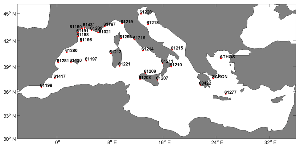
In situ measurements of H_s and T_m for 2014 were extracted from the Copernicus In Situ Thematic Assemble Centre (INS-TAC), a component of CMEMS which aims at providing a research and operational framework to develop and deliver in situ observations and derived products based on such observations. H_s measurements from 32 wave buoys within the Mediterranean Sea were available in the examined year. Figure 2 depicts their location and unique ID code. T_m measurements were available from a subset of the depicted buoys which excludes all the buoys offshore from the Italian coastline. To collocate model output and buoy measurements, in space model output was taken at the grid point nearest to the buoy location. In time, buoy measurements within a time window of ±1 h from model output times at 3 h intervals (0, 3, 6 …, etc.) were averaged. Prior to model–buoy collocation, the in situ observations were filtered so as to remove those values accompanied by a bad quality flag (quality flags included in the data files provided by the INS-TAC). After collocation, visual inspection of the data was carried out, which led to some further filtering of spurious data points. In addition, T_m data below 2 s were omitted from the statistical analysis since 0.5 Hz (T=2 s) is a typical cut-off frequency for wave buoys. It is noted that WAM, in contrast to the wave buoys, does not implement a high-frequency cut-off in the computation of T_m but instead includes a high frequency tail extending the calculation to infinity. As a result, model T_m is anticipated to be somewhat biased towards lower values compared to measured T_m.

Figure 3 Mediterranean Sea subregions for qualification metrics.

Satellite observations of significant wave height, H_s, and wind speed, U₁₀ (used to obtain H_s−U₁₀ quality associations), for the year 2014 were obtained from a merged altimeter wave height database set-up at CERSAT – IFREMER (France). This database contains altimeter measurements that have been filtered and corrected (Queffeulou and Croizé-Fillon, 2013). Here, measurements from three satellite missions, Jason-2, Cryosat-2, and SARAL, were used. To collocate model output and satellite observations, the first two were interpolated in time and space to the individual satellite tracks. For each track, corresponding to one satellite pass, along-track pairs of satellite measurements and interpolated model output were averaged over ∼50 km (0.5^∘) grid cells, centred at grid points of the forcing wind model (0.125^∘ × 0.125^∘). This averaging is intended to break any spatial correlation present in successive 1 Hz (∼7 km) observations and/or in neighbouring model grid output (Pierre Queffeulou, personal communication, 2015).

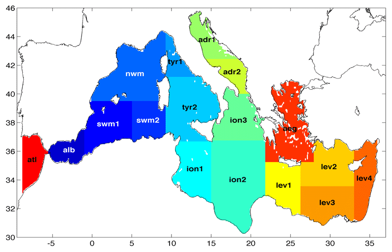
Metrics that are commonly applied to assess numerical model skill and are in alignment with the recommendations of the EU FP7 project MyWave (Saulter, 2014) have been used to qualify the Med-waves system within the Mediterranean Sea. These include the RMSE, bias, scatter index (SI), Pearson correlation coefficient (CORR), and best-fit slope (slope). The SI, defined here as the standard deviation of errors (model – observations) relative to the observed mean, as well as being dimensionless, is more appropriate to evaluate the relative closeness of the model output to the observations at different locations compared with the RMSE, which is representative of the size of a “typical” error. The slope corresponds to a best-fit line forced through the origins (zero intercept). In addition to the aforementioned core metrics, merged density scatter and quantile–quantile (QQ) plots are provided. Metrics are computed for the Mediterranean Sea as a whole, for the individual wave buoy locations shown in Fig. 2, and for 17 subregions of which one is in the Atlantic Ocean and 16 are in the Mediterranean Sea (Fig. 3): (atl) Atlantic, (alb) Alboran Sea, (swm1) West South-West Med, (swm2) East South-West Med, (nwm) North West Med, (tyr1) North Tyrrhenian Sea, (tyr2) South Tyrrhenian Sea, (adr1) North Adriatic Sea, (adr2) South Adriatic Sea, (ion1) South-West Ionian Sea, (ion2) South-East Ionian Sea, (ion3) North Ionian 3, (aeg) Aegean Sea, (lev1) West Levantine, (lev2) North-Central Levantine, (lev3) South-Central Levantine, and (lev4) East Levantine. All metrics are evaluated over a period of 1 year (2014). In addition, metrics associated with the full Mediterranean Sea are evaluated seasonally.

4 Validation results

4.1 Hindcast significant wave height

4.1.1 Comparison with in situ observations

Table 1 shows results of the comparison between hindcast H_s (model data) and in situ observations (reference data), for the Mediterranean Sea as a whole, for the entire year of 2014, and seasonally. In the table, “Entries” refers to the number of model–buoy collocation pairs; i.e. to the sample size available for the computation of the relevant statistics, $\overline{R}$ is the mean reference value, $\stackrel{\mathrm{‾}}{M}$ is the mean model value, and SD R and SD M are the standard deviations of the reference and model data respectively. The remaining quantities are the qualification metrics defined in the previous section. Figure 4 is the respective merged QQ–scatter plot (left), together with the QQ plot alone (right) for visual clarity, for the full 1-year period. In the figure, the QQ–plot is depicted with black crosses. Also shown are the best-fit line forced through the origin (red solid line, left plot) and the 45^∘ reference line (red dashed line).

Table 1 Med-waves H_s evaluation against wave buoy H_s, for the full Mediterranean Sea, for a 1-year period (2014) and seasonally.

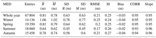
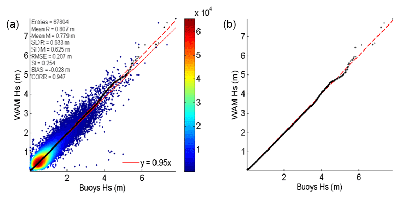
Figure 4 QQ–scatter plots (a) and QQ plot alone (b) of Med-waves output H_s versus wave buoy observations, for the full Mediterranean Sea, for a 1-year period (2014): QQ plot (black crosses), 45^∘ reference line (dashed red line), least-squares best-fit line (red line, a).

Table 1 shows that the typical error (RMSE) varies from 0.17 m in summer to 0.25 m in winter. However, the scatter in summer (0.26) is about 2 % higher than the scatter in winter (0.24) whilst a lower correlation coefficient is associated with the former season. This suggests that the model follows the observations in “stormy” conditions better, with well-defined patterns and higher waves. A similar conclusion has been derived by other studies (Cavaleri and Sclavo, 2006; Ardhuin et al., 2007; Bertotti et al., 2013) with respect to wind and wave modelling performance in the Mediterranean Sea. Like summer, autumn is characterized by lower mean wave height, higher scatter, and a lower correlation coefficient compared to winter and spring. Relative bias (BIAS/$\stackrel{\mathrm{‾}}{R}$) has an approximate variation of 2.5 % (spring) to 5 % (autumn) and is always negative. Accordingly, slopes are also below unity with small variation among seasons. These values are indicative of an underestimation of the wave height in the Mediterranean Sea by the model, a result which is in agreement with the results of a number of operational or preoperational models for the Mediterranean Sea (e.g. Bidlot, 2015; Donatini et al., 2015) and is linked to an underestimation of the wind speed by the ECMWF forcing wind model (see Fig. 7). Overall, the spring statistics are the ones closest to the year-long statistics for the Mediterranean Sea.

Figure 4 depicts the pattern of the agreement between hindcast and observed H_s for different H_s value ranges. The figure reveals that the H_s underestimation by the model mainly occurs for wave heights below 4 m and is rather small. It also shows a QQ plot that is really close to the reference line over most of the H_s range observed, which means that waves of a specific wave height have a very similar probability of occurrence in the hindcast and in the observations. The “outliers” present in the scatter plot, i.e. a number of measured waves of 2–4.5 m in height which are not simulated by the model (not enough evidence was found to remove the depicted outliers from the calculation of the statistics as faulty), correspond to buoy location 61218 in the Adriatic Sea (Fig. 2) and mostly belong to a single storm.

Table 2 Med-waves H_s evaluation against wave buoy H_s, for each individual buoy location, for a 1-year period (2014).

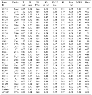
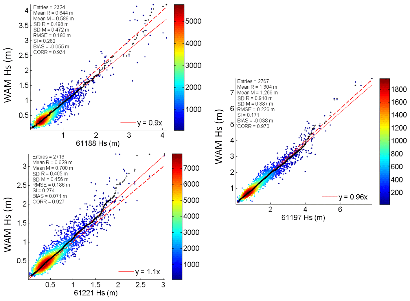
Figure 5 QQ–scatter plots of Med-waves output H_s versus wave buoy observations at specific wave buoy locations, for a 1-year period (2014): QQ plot (black crosses), 45^∘ reference line (dashed red line), and least-squares best-fit line (red line).

Table 2 shows results of the comparison between hindcast H_s and in situ observations for each of the wave buoys depicted in Fig. 2 (buoys listed from west to east). The table reveals that RMSE varies from 0.16 to 0.44 m with the highest values (>0.3 m) observed in the North Adriatic Sea at buoy location 61218 (0.44) and offshore of the French coastline at buoy location 61021 (0.35). Both locations are associated with poor overall qualification metrics, with location 61218 in particular displaying the poorest overall statistics. Thus, SI, which varies between 0.17 (61197) and 0.53 (61218), also obtains its highest values – indicating a poorer model performance – at locations within the North Adriatic Sea. Locations SARON and 61021 follow with values of 0.4 and 0.32 respectively. In general, SI values above the mean value for the whole Mediterranean Sea (0.25) are obtained at all wave buoys located near the coast that are sheltered by land masses to their west (e.g. western French coastline, eastern part of Corsica, and eastern part of Italy). With respect to the Italian buoys, this result is in close agreement with Cavaleri and Sclavo (2006), who found that the performance of the operational ECMWF wave model deteriorated at those Italian wave buoys facing east. This is because the resolution of the forcing wind model is not capable of reproducing the fine interaction between the prevailing north-northwesterly winds in the northern Mediterranean Sea with the complex orography sheltering the northern Mediterranean coastline well. An underestimation of wind speeds and consequently of wave heights (also the case herein) is commonly observed at such locations (Ardhuin et al., 2007). In addition, the buoys are often located only a few kilometres from the coastline; thus, in these conditions, i.e. when the wind is blowing from the coast, the approximation of the wave model grid size can lead to non-negligible fetch differences. Similar SI values are found within enclosed basins characterized by a complex topography such as the Adriatic and Aegean seas. In general, the closer the location to the coastline (e.g. 61187) and/or the more complex the surrounding topography (e.g. SARON), the poorer the model performance expected. As explained in several studies (e.g. Cavaleri and Sclavo, 2006; Bertotti et al., 2013; Zacharioudaki et al., 2015; Cavaleri et al., 2018), in these cases, the spatial resolution of the wave model is not adequate to resolve the fine bathymetric features, whilst, as mentioned above, the spatial resolution of the forcing wind model is incapable of reproducing the fine orographic effects, introducing errors to the wave hindcast. The correlation coefficient (CORR) largely follows the pattern of variation of the SI. It ranges from 0.79 (61218) in the Adriatic Sea to 0.98 (61213) at a location west of Sardinia which is well exposed to the prevailing north-westerly winds in the region. Bias varies from −0.13 m at location 61218 in the Adriatic Sea to 0.11 m at location 61021 offshore of the French coastline. It is mostly negative, indicating an underestimation of the observed wave height by the model, with positive bias observed at only six out of the 32 buoy locations examined. In most of the cases of relatively high positive bias, this is because the wave model resolution has missed or has partly captured important bathymetric features in the surroundings of the relevant locations, thus missing or reducing the shadowing effects produced by these features. For example, at shoreward buoy 61021 where the largest positive bias is observed, there are a few small islands that are almost entirely missed by the model. Also, at buoy 61221, similar to in Bertotti et al. (2013), the coastal geometry is not well represented by WAM. Bertotti et al. (2013) state that the buoy position is exposed to the easterly waves more than is actually the case, leading to the observed overestimate by the model. Similar conclusions stand for the SARON buoy in the Aegean Sea. Overestimation at buoy 61198 in the Alboran Sea is part of a general overestimation of the wave heights in the Atlantic and Alboran regions as it will be seen later in the comparison with the satellites. In accordance with bias, best-fit slopes (slope) vary from 0.77 at buoy location 61218 in the Adriatic Sea to 1.1 at buoy location 61021 offshore of France. Slope values above unity coincide with locations of positive bias; otherwise they are below unity, confirming an overall underestimation of the observations by the model. In general, the pattern of variation in slope is close to the pattern of variation in bias.

Table 3 Med-waves H_s evaluation against satellite H_s, for the full Mediterranean Sea, for a 1-year period (2014).

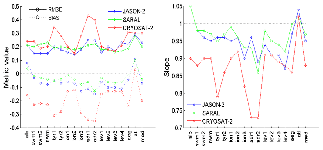
Figure 6 Med-waves H_s evaluation against satellite H_s, for each Mediterranean Sea subregion shown in Fig. 3, for a 1-year period (2014).

Up to now, the overall performance of the Med-waves modelling system at the different wave buoy locations has been analysed independently of the severity of the conditions. Figure 5, similar to Fig. 4, shows the QQ–scatter plots of hindcast H_s versus measured H_s at three buoy locations, exhibiting model performance over the different wave height ranges. The results at these three locations are reasonably representative of the different behaviours of the wave model at the different wave buoy locations in the Mediterranean Sea shown in Fig. 2. Thus, the top left plot shows the behaviour of the model at location 61188, offshore from the border between France and Spain, backed on the west by the Pyrenees Mountains. It is seen that model underestimation occurs throughout the measured H_s range except from the highest percentiles of H_s at which model overestimation is observed. This distribution, with a smaller or larger model underestimate and with a more or less pronounced convergence or overestimate towards the highest waves, is observed at the majority of the wave buoy locations. The bottom left plot corresponds to location 61221, south of the island of Sardinia. There, the model overestimates the observed H_s over the entire H_s range, even more so in the upper end of this range. Considerable model overestimation, mostly over the middle and higher H_s ranges, is observed at all wave buoys associated with unresolved bathymetric features in their surroundings (e.g. 61021, SARON). Over the lower H_s range, convergence or underestimation is also observed in these conditions. At SARON (not shown), the surrounding topography is highly complex, including both orographic and bathymetric effects, resulting in highly scattered data around the reference line. The right plot shows results at buoy location 61197 east of the Balearic Islands. This is a well-exposed offshore wave buoy; consequently, the behaviour of the model at this location is expected to be representative of its performance at well-exposed offshore sites. Relatively small scatter of the data points is shown in the plot with QQ crosses and the best-fit line laying close to the reference line. More specifically, the model converges to the observations for wave heights below about 2 m, somewhat underestimates the observations for wave heights between 2 and 4 m, and tends to overestimate H_s for higher waves. A very similar distribution is found for location 61430 west of the Balearic Islands. Other well-exposed offshore locations present QQ–scatter patterns that are not far from the one shown for location 61197.

4.1.2 Comparison with satellite observations

This subsection starts with the comparison of Med-waves hindcast H_s with satellite observations of H_s separately for each satellite. This is carried out for a 1-year period (2014) for the full Mediterranean Sea and for the different subregions defined in Fig. 3. Respective results are shown in Table 3 and Fig. 6.

Table 3 shows that even though the model–satellite comparison behaves similarly for the three different satellites in terms of SI and CORR, a substantially more (>10 %) negative model bias associated with a considerably lower slope is found for Cryosat-2. RMSE is also higher for this satellite. Figure 6 shows that these results are largely consistent among the different Mediterranean subregions although they are more pronounced in the western Mediterranean and the Adriatic Sea. A lower model underestimate of the Cryosat-2 measurements is observed in the Ionian Sea and the eastern Mediterranean. The statistics of model–Jason-2 and model–SARAL comparisons are comparable, with the model exhibiting its best performance when compared to the observations of SARAL.

Table 4 Med-waves H_s evaluation against satellite H_s (Jason-2 and SARAL), for the full Mediterranean Sea, for a 1-year period (2014) and seasonally.

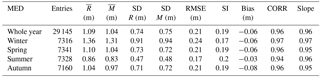
Figure 7 QQ–scatter plots of (a) ECMWF forcing wind speed U₁₀ versus satellite U₁₀ (Jason-2) and (b) Med-waves H_s versus satellite H_s (Jason-2 and SARAL), for the full Mediterranean Sea, for a 1-year period (2014).

It was decided to exclude the observations of Cryosat-2 from the analysis. Apart from the aforementioned discrepancies, there are other results in the literature to support this decision. Specifically, satellite–buoy comparisons performed by Sepulveda et al. (2015) have shown that SARAL H_s is of better quality than Jason-2 and Cryosat-2 H_s at both open-ocean and coastal buoy sites. In fact, SARAL data are of very high quality with no need of corrections whilst corrections are applied to Jason-2 and Cryosat-2 H_s observations (corrected data are used herein). After corrections, Jason-2 H_s has been found to approximate SARAL H_s well whilst less accurate results have been obtained for Cryosat-2, particularly for wave heights below 1.5 m. For these reasons, in what follows, the comparison of Med-waves H_s is performed against merged satellite observations from the SARAL and Jason-2 satellites, which are of similar accuracy.

Table 4 shows statistics from the comparison of the Med-waves hindcast H_s and satellite observations of H_s, for the full Mediterranean Sea, for a 1-year period and seasonally. Figure 7b shows the corresponding QQ–scatter plot for a 1-year period, for the full Mediterranean Sea. Figure 7a shows an equivalent QQ–scatter plot resulting from the comparison of the ECMWF forcing wind speeds, U₁₀, and Jason-2 measurements of U₁₀ (no U₁₀ available from SARAL or Cryosat-2).

Figure 7a shows that the ECMWF forcing wind model mostly underestimates observed U₁₀, even more so at high wind speeds. An overall model underestimation of 8 % associated with a slope of 0.9 has been computed. Figure 7b also shows an overall Med-waves model underestimation of observed H_s by about 5 % associated with a slope of 0.96. Nevertheless, in this case, the model somewhat underestimates observed H_s over the lower H_s range (<2 m), converges to the observed H_s over the middle H_s range (2–3.5 m), and, generally, somewhat overestimates the larger waves in the data records. This apparent discrepancy between wind and wave scatter distributions is a consequence of the modification of the default values of the whitecapping dissipation coefficients in WAM as described in Sect. 3. A QQ–scatter plot obtained before this modification (not shown) is indeed very similar to the one of the ECMWF wind speeds in Fig. 7. On the whole, Fig. 7 shows that the performance of Med-waves at offshore locations in the Mediterranean Sea (satellite records near the coast are mostly filtered out as unreliable) is very good. Comparing to the equivalent results obtained from the model–buoy comparison (Fig. 4), a very similar pattern of scatter distribution is observed in the two plots, also evident from the orientation of the best-fit lines and the curvature of the QQ plots. A smaller scatter (by about 6 %) with a larger overall bias (by about 2 %) is associated with the model–satellite comparison. SI values compare well at the more exposed wave buoys in the Mediterranean Sea.

Table 5 Med-waves H_s evaluation against satellite H_s (Jason-2 and SARAL), for each individual Mediterranean Sea subregion shown in Fig. 3, for a 1-year period (2014).

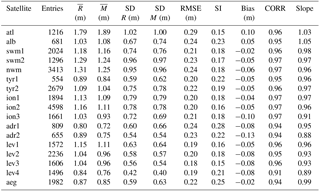
Table 4 shows the seasonal variation in the Med-waves model performance. RMSE varies from 0.17 m in summer to 0.24 m in winter. SI is highest in summer (0.2) and lowest in winter (0.17). Correlation coefficient varies accordingly. In general, as explained in the previous subsection, a lower scatter with a higher correlation is expected the more well-defined the weather conditions are. Similar to in the model–buoy comparison, bias is negative in all seasons. Its highest relative value (BIAS/$\stackrel{\mathrm{‾}}{R}$) of 7.7 % is computed for autumn and its lowest of 3.5 % for summer. Slope varies from 0.95 in spring and autumn to 0.97 in winter. Overall, Table 4, like Table 1, reveals that the statistics of spring are the most representative of the year-long statistics for the Mediterranean Sea.

Table 5 shows the statistics of the comparison of the Med-waves hindcast H_s and satellite observations of H_s for the different subregions of the Mediterranean Sea defined in Fig. 3. For visualization purposes, Fig. 8b maps the statistics shown in Table 5. In addition, equivalent statistics are mapped for the ECMWF – satellite comparison of wind speeds (Fig. 8a). It is noted that the relative bias (BIAS/$\stackrel{\mathrm{‾}}{R}$) is displayed in the figure. This quantity allows for a more straightforward comparison among the different sub-basins in terms of percentage deviations from the observed mean value. It is also highlighted that the spatial coverage of the model–satellite wind collocations (measurements only from Jason-2) is much more limited than the spatial coverage of the model–satellite wave collocations (measurements from both SARAL and Jason-2). As a consequence, the wave statistics are expected to be more representative of the subregions under consideration compared to the wind statistics. This is particularly true for the Adriatic, the Ligurian, and the Alboran Seas. In addition, the wave statistics have been computed using a sample size of at least 400 data points whilst the wind statistics have been obtained with a minimum sample requirement of 200 data points. Thus, the confidence associated with the wave statistics is higher than the confidence associated with the wind statistics. For the above reasons, the wind metrics presented in Fig. 8 are interpreted with caution.

Figure 8 ECMWF U₁₀ (a) and Med-waves H_s (b) evaluation against satellite U₁₀ (Jason-2) and satellite H_s (Jason-2 and SARAL) respectively: maps of metric values over the Mediterranean Sea subregions shown in Fig. 3, for a 1-year period (2014).

Figure 8b shows that the typical error (RMSE) varies from 0.18 m in the South-Central Levantine Basin (lev3 in Fig. 3) to 0.24 m in the Alboran Sea, the North West Mediterranean (nwm), and the North Adriatic subregions up to 0.29 m in the Atlantic subregion. In terms of SI, the highest value (0.28) is obtained in the North Adriatic Sea followed by the Aegean Sea (0.24). The South Adriatic, Alboran, Ligurian (tyr1), and East Levantine (lev4) seas also have relatively high SI values (0.21–0.23). The lowest values are found over the south-eastern Mediterranean Sea (0.15–0.16) and in the Atlantic subregion (0.15). SI and CORR have a similar pattern of variation, a notable difference being that the correlation coefficient obtains its worst value in the East Levantine and, in general, it has relatively lower values in the well-exposed regions of the Levantine Basin compared to the well-exposed regions to its west. In accordance with the above results, Ratsimandresy et al. (2008), examining model–satellite agreement over coastal locations of the western Mediterranean Sea, found the worst correlations in the Alboran Sea and east of Corsica. Bertotti et al. (2013), in a comparison of high-resolution wind and wave model output with satellite data over different subregions of the Mediterranean Sea, also found the largest scatter and lowest correlations in the Adriatic and the Aegean seas. In agreement, Zacharioudaki et al. (2015), focusing on the Greek seas, have shown a considerably larger scatter in the Aegean Sea than in the surrounding seas when model output was compared to satellite observations. As explained in the previous subsection (model–buoy comparison), it is difficult for wind models to reproduce orographic effects and/or local sea breezes well and difficult for wave models to resolve complicated bathymetry that introduces errors in these fetch-limited, enclosed regions, often characterized by a complex topography, well. Indeed, comparison with the equivalent results for the ECMWF wind speeds confirms these difficulties. For example, the pattern of SI and CORR variation for U₁₀ largely resembles that for H_s, corroborating the conclusion of many studies that errors in wave height simulations by sophisticated wave models are mainly caused by errors in the generating wind fields (e.g. Komen et al., 1994; Ardhuin et al., 2007). Nevertheless, some differences do exist. For instance, the H_s SI in the Aegean Sea is relatively higher than the corresponding U₁₀ SI. This is most probably because in this region of highly complicated bathymetry with many little islands the error of the wave model increases in relation to the error of the wind model. Similarly, in the East Levantine, H_s SI is lower than that implied by U₁₀ SI. In this case, the wind model may not simulate local wind patterns, characterized by local sea breezes and easterly directions, well (Galil et al., 2006); however, the wave regime which is dominated by waves from the west sector (Galil et al., 2006) is better reproduced by the wave model. Negative bias and slope below unity are the case in all subregions except for the Atlantic Ocean and Alboran Sea.

Table 6 Med-waves T_m evaluation against wave buoys' H_s, for the full Mediterranean Sea, for a 1-year period (2014) and seasonally.

In the last two regions, the wave model overestimates the observations by 5 %–6 %. Otherwise, it underestimates the observations by about 2 % in the East South-West Mediterranean (swm1) and Aegean seas to about 15 % in the Adriatic (adr2). In general, the largest biases are found in the Adriatic (adr1, adr2), the North Ionian Sea (ion3), and the Levantine Basin (lev2, lev3, lev4) with values of 7.5 %–15.2 %. Slope varies accordingly with values between 0.88 in the South Adriatic Sea (adr2) and 0.99 in the Aegean Sea and up to 1.05 in the Alboran Sea. Comparing with the equivalent results for the ECMWF wind speed, it is evident that although there are similarities in the relative bias and slope distributions, there are also considerable differences. In general, in terms of absolute value, the relative bias associated with the wind field is larger than that associated with the wave field except for the South Adriatic Sea, the Alboran Sea, and the Atlantic. In fact, in the last two regions, a change of sign from negative to positive is observed between wind and waves. As already mentioned, this is a consequence of the modification of the whitecapping dissipation coefficients from default values in WAM, which has led to an important offset of the negative bias associated with the ECMWF wind speeds, especially over the high H_s range. Thus, in regions where the ECMWF underestimate has been small, as in the Atlantic, modification of the dissipation coefficients has eventually led to an overshoot of the observed H_s. This is a robust pattern obtained for the whole Atlantic area simulated by the nested Med-waves model (up to −18.125^∘ W; Fig. 1). The increase in negative H_s relative bias in the South Adriatic Sea relative to the respective U₁₀ relative bias is somewhat puzzling; however, as mentioned above, small confidence pertains to the results of U₁₀ in the Adriatic Sea due to a limited observational coverage by Jason-2.

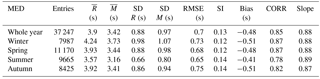
4.2 Hindcast mean wave period

Table 6 presents the statistics of the comparison between the Med-waves hindcast mean wave period, T_m, and in situ observations of mean wave period, for the full Mediterranean Sea, for a 1-year period (2014) and seasonally. Figure 9 shows the corresponding QQ–scatter plot for the year-long statistics. It is shown that the model exhibits greater variability than the observations (SD in Table 6). RMSE varies from 0.8 s in summer to 1.07 s in winter. In relation to the mean of the observations, the error is about 17 %–19 %, with winter and spring being at the low end of this range and autumn at the high end. SI varies from 0.12 in winter and spring to 0.14 in summer and autumn. The non-trivial deviation of SI from relative RMSE (RMSE/$\stackrel{\mathrm{‾}}{R}$) indicates that a substantial part of the error is caused by bias. CORR has its minimum value (0.78) in summer and its maximum (0.87) in winter and spring. As before, these results indicate that the model wave period, like the model wave height, better follows the observations in well-defined wave conditions of higher waves and larger periods. Bias is negative with values that correspond to a model underestimate of about 11.5 %–13 %. Correspondingly, slope has a small variation of 0.87–0.89. Like for wave height, spring statistics are the most representative of the year-long statistics. Figure 9 clearly shows that the wave model underestimates the observations throughout the observed T_m range. Measurements of T_m<4.5 s are especially underestimated while those of relatively high T_m are better approximated by the model. As mentioned in Sect. 3, part of the model underestimation of observed T_m, especially over the lower T_m range, may be attributed to the absence of a high frequency cut-off in the model in contrast to the observations.

Figure 9 QQ–scatter plots of Med-waves output versus wave buoy observations, for the full Mediterranean Sea, for a 1-year period (2014).

Table 7 Med-waves T_m evaluation against wave buoy T_m, for each individual buoy location, for a 1-year period (2014).

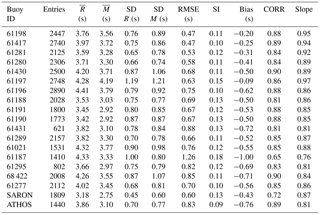
Table 7 gives the statistics of the model–buoy comparison at the individual wave buoy locations. The typical error relative to the mean of the observations (RMSE/$\stackrel{\mathrm{‾}}{R}$) has its lowest values of 12 %–16 % over the western part of the Mediterranean Sea, west and south of France, with the two locations nearest to the Gibraltar Straight being at the low end of this range. Otherwise, this error is 17 %–23 %, reaching up to 29 % at location 61187 near the French–Italian border. At this location, all qualification metrics obtain their worst value. This is because wave buoy 61187 is located at a distance less than 2 km from coast and is affected by winds blowing from land. As already explained in the model–buoy wave height comparison, in this situation, the simulated fetch may differ substantially from the actual fetch because of the wave model grid size approximation; moreover, wind speed and wave height are considerably underestimated. RMSE is mainly caused by bias, which is negative at all locations. Thus, according to the RMSE, the relative bias is below 10 % over the western Mediterranean and is 14 %–20 % otherwise reaching up to 23 % at location 61187. It is only at location 61197, offshore from the eastern Balearic Islands, that the scatter of the data appears to contribute more to the typical error than the bias. This is a well-exposed offshore location where bias (2 %) and slope (0.97) have their best values and where model performance has been found to be optimal for wave height. The relatively high SI (0.15) and moderate correlation (0.86) at this location could be associated with the appearance of two density peaks in the density scatter plot (not shown), indicative of a double-peaked frequency spectrum. Density scatter plots with two peaks, although less distinct, have also been obtained for locations 61289 and 61021, offshore from France. In general, a close examination of the QQ–scatter plots (not shown) corresponding to the different locations has revealed that the model largely underestimates the observed T_m over the lower wave period range at all locations. Over the higher range, the model converges or overestimates the observed T_m in the western Mediterranean Sea, west and south of France. Otherwise, the model underestimates all observed T_m values with some convergence towards higher values. Slope mostly follows the pattern of variation in bias with values between 0.76 and 0.97. SI is relatively small with values between 0.09 (ATHOS) and 0.18 (61187) while CORR varies from 0.65 (61187) to 0.9 (61430, 68422). Generally, similar to the wave height results, the lowest correlations are found at coastal locations affected by fetch differences between model and reality due to a complex surrounding topography. Conversely, the highest correlations are obtained at the most exposed wave buoy locations.

4.3 Forecast skill

In the previous section, the performance of the Med-waves system has been characterized through the comparison of hindcast wave parameters with observations. In this section, the forecast skill of the Med-waves system is explored by comparing forecast wave parameters with observations at different forecast lead times. Hence, Fig. 10 shows Med-waves forecast skill for H_s (Fig. 10b, c) together with ECMWF forecast skill for U₁₀ (Fig. 10a). The latter is evaluated against satellite observations, the former is evaluated against satellite (Fig. 10b) and buoy (Fig. 10c) observations. It is noted that in the model–buoy comparisons, each lead time represents a single point in time, whist, in the model–satellite comparisons, each lead time represents a full forecast day; i.e. +0 h represents forecast day 1 containing data from 0 to 24 h forecast. This approach is dictated by the scarcity of satellite observations in time.

Figure 10 ECMWF U₁₀ forecast skill evaluated against satellite observations (a) and Med-waves H_s forecast skill evaluated against satellite (b) and buoy (c) observations, for the full Mediterranean Sea, for a 1-year period (2014).

Figure 11 Med-waves T_m forecast skill evaluated against buoy observations, for the full Mediterranean Sea, for a 1-year period (2014).

Figure 10 shows that H_s SI grows with forecast lead time at a constantly increasing growth rate. At the same time, CORR decreases with forecast lead time, with the decrease being more notable after the third day of forecast (+48 h). These patterns, which are consistent between model–buoy and model–satellite observations, mostly agree with the equivalent U₁₀ patterns and manifest the deterioration of the forecast in time. A small difference between U₁₀ and H_s forecast skill is the somewhat more linear increase in SI with forecast lead time in the first case, which results in a smaller overall U₁₀ deterioration over the length of the forecast (14 %) compared to the respective H_s deterioration (19 % for model–satellite comparisons). This is indicative of the sensitivity of wave height to even limited variations in the input wind intensity. Conversely, waves seem to be less sensitive to wind misfits in time and space, which is manifested by the higher and more persistent H_s CORR over the forecast range compared to the respective U₁₀ CORR. Contrary to SI and CORR but also to U₁₀ bias, the evolution of H_s bias with forecast lead time in not monotonic. This apparent discrepancy between wind and wave bias evolution is attributed to the modification of the default values of the whitecapping dissipation coefficients in WAM, which, as shown in Sect. 4.1.2, have an impact on the bias of the wave model output relative to the observations. In any case, for both winds and waves, the variation in bias with forecast range is small and does not exceed 2 %.

Figure 11, like Fig. 10c, shows Med-waves forecast skill for T_m evaluated against wave buoy observations. Similar to H_s, SI increases with forecast range, CORR decreases, and bias exhibits a non-monotonic variation analogous to the one of H_s. In this case however, the variation in SI over the forecast period is small (5 %) compared to the respective H_s variation (25 %). This agrees with the finding that T_m errors are mainly caused by bias (Sect. 4.2).

5 Conclusions

The CMEMS Mediterranean wave forecasting system, Med-waves, has been operational since April 2016, providing short-range forecasts over the Mediterranean Sea at hourly intervals and at a horizontal resolution of 1∕24^∘. The development and the evaluation of the performance of the system has been presented in detail in this paper. In the framework of this evaluation, the wave parameters of significant wave height and mean wave period have been evaluated against in situ and satellite observations over a period of 1 year (2014). Both hindcast quality and forecast skill have been assessed. In the former case, evaluation statistics have been provided for the Mediterranean Sea as a whole, at individual buoy locations and over predefined Mediterranean subregions. In the latter case, evaluation statistics have been provided only for the entire Mediterranean Sea. The main findings of this evaluation assessment are summarized below.

Overall, the significant wave height is accurately simulated by the model. Considering the Mediterranean Sea as a whole, the RMSE is 0.21 m and the bias is −0.03 m (3.7 %) when the model is compared to in situ observations and −0.06 m (5.5 %) when it is compared to satellite observations. In general, the model somewhat underestimates the observations for wave heights below 4 m whilst it mostly converges to the observations for higher waves. The scatter index, indicative of the scatter of the data around their regression line, is 25 % for the model–in situ comparison and 19 % for the model–satellite comparison, demonstrating a reduced scatter off the shore (where satellite measurements are mostly located) compared to near the shore (where in situ measurements are mostly obtained). The correlation coefficient is 0.95–0.96 and so is the best-fit slope. Model performance is better in winter when the wave conditions are well defined. Spatially, the model performs optimally at offshore wave buoy locations and well-exposed Mediterranean subregions. Within enclosed basins and near the coast, unresolved topography by the wind and wave models and fetch limitations cause the wave model performance to deteriorate. In particular, the model has an optimal performance along most of the southern Mediterranean Sea. Its performance is less good in the Alboran, Ligurian, Adriatic, Aegean, and Eastern Levantine seas, with the worst evaluation statistics obtained in the Adriatic. In terms of bias, the model overall underestimates the measurements in the Mediterranean Sea. The smallest underestimate is observed in the Aegean Sea while overestimate is observed in the Alboran Sea and in the Atlantic.

Poor wave model statistics were strongly linked to poor wind forcing statistics. Naturally, it is expected that an improved orographic representation of the ECMWF forecasting system will improve the quality of the surface wind fields near the coast while a higher temporal resolution of wind forcing would be beneficial to the model to resolve the high wind and wave variability in the Mediterranean Sea, providing more accurate wave fields. Moreover, the atmospheric model of ECMWF, which was not coupled with an ocean model (coupling was performed only with the wave component) by the time of this study, did not consider some vigorous air–sea interaction processes (large heat fluxes or strong ocean mixing processes) that occur in regions which are usually affected by extreme weather events such as the northern part of the Adriatic during strong wind events (Bora, Sirocco). As a result, it failed to properly reproduce the spatial structure of the wind fields. To overcome this limitation, many studies (Carniel et al., 2016; Ricchi et al., 2016, 2017) show that the use of a fully coupled atmosphere–ocean–wave model can be considered appropriate for these regions for properly representing the air–sea interactions and for providing a more realistic and consistent evolution of the atmospheric and oceanic fields. It is noted at this point that substantial progress has been made since the year 2014 – the year the results of this study are obtained for – by ECMWF regarding spatial and temporal resolutions and coupling. Specifically, the spatial resolution of the ECMWF winds has increased since spring 2016 from 16 to 9 km. Also, in June 2018, it was decided that ECMWF can provide hourly forecasts up to a forecast step of 90 h (Jean Bidlot, personal communication, 2018). Finally, in June 2018, the ECMWF forecasting system is a fully coupled atmosphere–waves–ocean–sea ice system (ECMWF, 2018). As a consequence of these improvements, a future validation of the Med-waves system is expected to yield better validation results.

The mean wave period is reasonably well simulated by the model. The RMSE is 0.7 s and is mainly caused by model bias, which has a value of −0.48 s (12 %). In general, the model underestimates the observed mean wave period and exhibits greater variability than the observations. A relatively larger model underestimate is found for mean wave periods below 4.5 s. The scatter index is 13 %, the correlation coefficient is 0.85 and the best-fit slope is 0.88. Model performance is a little better in winter when wave conditions are well defined. Spatially, the model somewhat overestimates the highest mean wave period values in the western Mediterranean Sea, west and south of France. Otherwise, model underestimate is widespread. Similar to the wave height, the model performance is best at well-exposed offshore locations and deteriorates near the shore mainly due to fetch limitations.

The forecast skill of the model over the Mediterranean Sea deteriorates with forecast range. The growth of error in the wave forecast is mainly due to the growth of error in the forcing wind fields. The scatter index of the significant wave height deteriorates by 19 and 25 % over the 5-day forecast for model–satellite and model–buoy comparisons respectively. The equivalent deterioration for mean wave period is only 5 % (model–buoy comparison). A monotonic decrease in correlation is also observed. On the contrary, the evolution of bias with forecast range shows some variability with no clear trend. Nevertheless, this variability does not exceed 3 % over the forecast period.

In the next version of the system an optimal interpolation data assimilation scheme is added to the Med-waves system in order to blend satellite along-track significant wave height measurements with model background forecasts. Although wave data assimilation is known not to be particularly beneficial in areas where wind sea conditions are dominant, we expect that wave forecasts in certain sub-areas of the Mediterranean Sea where swell propagation is quite frequent, will be improved at +24 h and perhaps +48 h lead time. The enhanced Med-waves system with the data assimilation system module is going to produce 3-hourly wave analyses on a daily basis for the Mediterranean Sea by assimilating Sentinel-3 and Jason-3 altimeter measured significant wave heights and surface winds. The assimilation is based on the inherent data assimilation scheme of WAM Cycle 4.5.4 model, which generates an updated wave field by distributing the information from the observed significant wave height and surface wind data within a given time window over the entire model grid. The Med-waves data assimilation component is integrated into the Med-waves system since April 2018.

Lastly, more work will be devoted to improve the offline coupling between waves and currents by including as a next step the variations in the sea level as predicted by the physical component of the Med MFC system. In parallel the full online two-way coupling between Mediterranean waves and currents will be developed and implemented into the Med MFC system, with a target to enter into the operational chain in future versions of the Copernicus Marine Service, improving the forecasting skill of the models in various coastal areas of the basin.