the Creative Commons Attribution 4.0 License.
the Creative Commons Attribution 4.0 License.
 | 18 Oct 2018
Convection-permitting regional climate simulations for representing floods in small- and medium-sized catchments in the Eastern Alps
Christian Reszler
Matthew Blaise Switanek
Heimo Truhetz
Small-scale floods are a consequence of high precipitation rates in small areas that can occur along frontal activity and convective storms. This situation is expected to become more severe due to a warming climate, when single precipitation events resulting from deep convection become more intense (super Clausius–Clapeyron effect). Regional climate model (RCM) evaluations and inter-comparisons have shown that there is evidence that an increase in RCM resolution and, in particular, at the convection-permitting scale will lead to a better representation of the spatial and temporal characteristics of heavy precipitation at small and medium scales. In this paper, the benefits of grid size reduction and bias correction in climate models are evaluated in their ability to properly represent flood generation in small- and medium-sized catchments. The climate models are sequentially coupled with a distributed hydrological model. The study area is the Eastern Alps, where small-scale storms often occur along with heterogeneous rainfall distributions leading to a very local flash flood generation. The work is carried out in a small multi-model framework using two different RCMs (CCLM and WRF) in different grid sizes. Bias correction is performed by the use of the novel scaled distribution mapping (SDM), which is similar to the usual quantile mapping (QM) method. The results show that, in the investigated RCM ensemble, no clear added value of the usage of convection-permitting RCMs for the purpose of flood modelling can be found. This is based on the fact that flood events are the consequence of an interplay between the total precipitation amount per event and the temporal distribution of rainfall intensities on a sub-daily scale. The RCM ensemble is lacking in one and/or the other. In the small catchment (<100 km2), a favourable superposition of the errors leads to seemingly good CCLM 3 km results both for flood statistics and seasonal occurrence. This is, however, not systematic across the catchments. The applied bias correction only corrects total event rainfall amounts in an attempt to reduce systematic errors on a seasonal basis. It does not account for errors in the temporal dynamics and deteriorates the results in the small catchment. Therefore, it cannot be recommended for flood modelling.
- Article
(11724 KB) - Full-text XML
-
Supplement
(1148 KB) - BibTeX
- EndNote


Floods in small- and medium-sized catchments are often triggered by atmospheric processes on small scales, i.e. small-scale frontal systems (Schemm et al., 2016) and convective storms. In the Austrian Alpine area, these types of small-scale storms cause millions of Euros in damage every year. This situation is expected to become more severe as a result of a warming climate and the Clausius–Clapeyron relationship. Single precipitation events are expected to become more intense (e.g. Allen and Ingram, 2002; Trenberth et al., 2003; Allan and Soden, 2008; Gobiet et al., 2014), and recent investigations have shown increases in deep convective precipitation can exceed the Clausius–Clapeyron relationship (known as the super Clausius–Clapeyron scaling effect, e.g. Lenderink and Van Meijgaard, 2009; Berg et al., 2013; Wang et al., 2017; Lenderink et al., 2017).
Regional climate models (RCMs) are valuable tools for studying climate change effects on water resources. They are employed to generate climate simulations at scales below a 50 km horizontal resolution, like in the EU-FP7 project ENSEMBLES (Hewitt and Griggs, 2004) or the North American Regional Climate Change Assessment Program (NARCCAP) (Mearns et al., 2009). RCMs operating with 0.11∘ (∼12 km) grid spacing became the standard in Europe as a result of EURO-CORDEX (https://www.euro-cordex.net/, last access: 15 October 2018) (Jacob et al., 2014, which is the ongoing European branch of the global Coordinated Regional Downscaling Experiment – CORDEX (Giorgi et al., 2009) of the World Climate Research Programme – WCRP). Prein et al. (2016) investigated the added value in precipitation in the EURO-CORDEX RCMs. They demonstrated that as model resolution increased, atmospheric processes such as extreme precipitation are more realistically represented, especially in regions of complex terrain (e.g. the Alpine region). Nissen and Ulbrich (2017) focused on the representation of heavy precipitation events in the EURO-CORDEX ensemble. They found that the frequency and size of heavy precipitation events are predicted to increase over most of Europe with increasing greenhouse gas concentrations. Moreover, the most severe events were detected to be in the projection period.
With improvements in numerical weather prediction (NWP) and computing technology, RCM grid spacing can now be further reduced to allow convection-permitting climate simulations (CPCSs). CPCSs benefit from two major advantages with respect to precipitation extremes: (1) deep moist convection, which is the most important process in the majority of extreme precipitation events, is physically resolved by the RCM; and (2) the representation of orography and surface fields is improved. Multiple studies have already demonstrated the added value of convection-permitting models (CPMs, Prein et al., 2015) in capturing extreme precipitation (e.g. Chan et al., 2013, 2014, 2016; Meredith et al., 2015; Zittis et al., 2017) and their frequency of occurrence (Ban et al., 2014; Knist et al., 2018). However, there are only a few future projections that use CPCSs, like Prein et al. (2017), Ban et al. (2015), Kendon et al. (2014), and Knist et al. (2018). Although processes are better represented in CPCSs, local biases are not necessarily being reduced. Their bandwidths are large and (spatial and temporal) correlation coefficients are poor when they are compared to highly resolved observation data (e.g. Prein et al., 2013; Ban et al., 2014; Knist et al., 2018). In particular, Ban et al. (2014) and Knist et al. (2018) found that their models (CCLM and WRF) increasingly overestimate extreme events in mountainous regions. This makes bias-correction techniques indispensable, even if deep convection becomes resolved by RCMs. Also, additional computational costs for the convection-permitting simulations are high, which can limit their application, in particular for climate change studies in decision making (e.g. uncertainty assessment by ensemble simulations).
Hinging on the scale of the driving data, climate change impact studies have often focussed on water balance in relatively large catchments (e.g. Fowler et al., 2007). Regarding floods, numerous studies were performed and pointed out the high uncertainties in the GCM–RCM–hydrological-model chain (e.g. Hennegriff et al., 2006; Dankers et al., 2007; Hanel and Buishand, 2010). Maraun et al. (2010) provided a comprehensive review on the requirements of hydrological models and their fulfilment via RCMs. They define the requirements in a correct representation of (1) intensities, (2) temporal variability, (3) spatial variability and (4) consistency between different local-scale variables. Köplin et al. (2014) used future climate change scenarios from the ENSEMBLES project to analyse the seasonality and magnitude of floods in Switzerland. They found that the simulated change in flood seasonality is a function of the change in flow regime type. Magnitudes of both mean annual floods and maximum floods (in a 22-year period) are expected to increase in the future because of changes in flood-generating processes and scaled extreme precipitation. Using the new EURO-CORDEX models Alfieri et al. (2015) assessed projected changes in flood hazard in Europe based on the RCP8.5 scenario and the hydrological LISFLOOD model. Their results indicate that the change in frequency of discharge extremes is likely to have a larger impact on the overall flood hazard as compared to the change in their magnitude. On average, in Europe, flood peaks with return periods above 100 years are projected to double in frequency within 3 decades. In an effort to sequentially couple convection-permitting RCMs with a hydrological model, first attempts have been made. For example, Kay et al. (2015) use results of a 1.5 km RCM nested in a 12 km RCM driven by European reanalysis boundary conditions to drive a gridded hydrological model. However, they found that the 1.5 km RCM generally performs worse than the 12 km RCM for simulating river flows in 32 example catchments.
In this study, two regional climate models (CCLM and WRF) with different grid spacing (∼50, ∼12.5 and ∼3 km) are sequentially coupled (one way) with a hydrological model for representing floods on small and medium spatial scales (30 to 1000 km2). An improved bias-correction technique (Switanek et al., 2017) is used to minimise error propagation throughout the modelling chain. The study area is located in south-eastern Austria (Styria), where local flash floods are the predominant flood type (e.g. Merz and Blöschl, 2003). The spatially distributed hydrological model KAMPUS (Blöschl et al., 2008) is used, which is in operational use for flood forecasting in Austria in small- to medium-sized scales (Blöschl et al., 2008; Ruch et al., 2012). The added value of the highly resolved convection-permitting RCM set-up (∼3 km grid spacing) is evaluated in the period 1989–2010 by quantitative and qualitative criteria regarding flood generation.
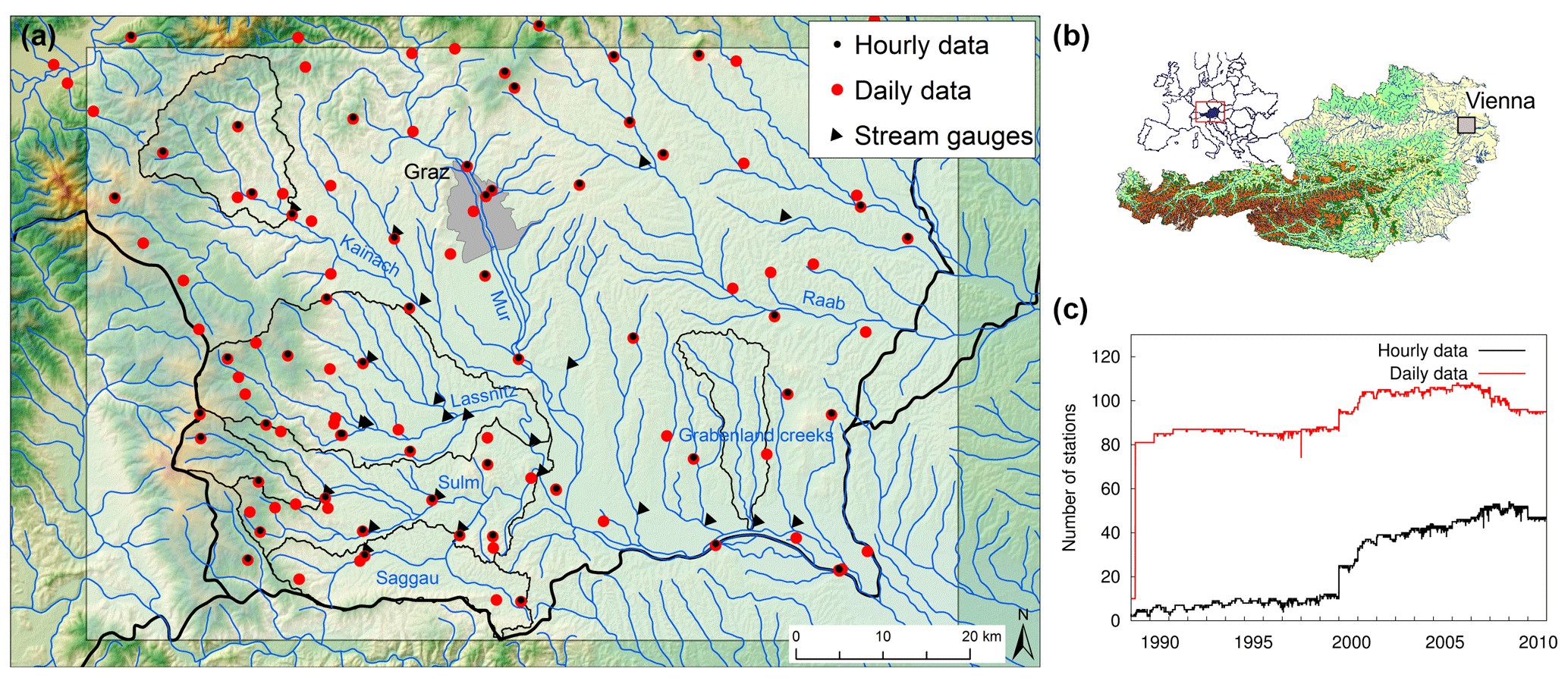
Figure 1Study area and station distribution (a) as well as availability of high-resolution meteorological data (c). Polygons are the catchment boundaries of the stream gauges for evaluation in this study (Table 1, Fig. 3).
The study area is located in south-eastern Austria, at the border of the Eastern Alps (Fig. 1). Meteorological data of all available stations in the region were acquired from the Hydrographic Service of the provincial government of Styria and the Austrian Central Institute for Meteorology and Geodynamics (ZAMG). Figure 1 shows the distribution of the stations during the period 2000 to 2009, which corresponds to the calibration period of the hydrological model. Data coverage has improved through the years by installing new stations. Historically in Austria, the network of stations with daily data (ombrometer) is much denser than the network of stations with high temporal recording (e.g. every 15 min or hourly). In the bottom right plot the development of the station availability in southern Styria is shown. At the beginning of 2000 the number of stations with high temporal resolution significantly increased, whereas the number of stations with daily data was high since the beginning of the study period in 1989.
Interpolated fields of precipitation and air temperature are generated on an hourly basis. Stations with daily data are incorporated into the interpolation procedure to benefit from the dense network as follows (Reszler et al., 2006): first, daily data are interpolated on the model grid (1 km). Then, hourly data are interpolated on the same grid and the daily sum of the cells is calculated and scaled to the daily grid. Spatial distribution of daily precipitation is expected to be accurate even in the years before 2000, which is important for an accurate representation of the general water balance. However, due to the high spatial variability of precipitation in the region, hourly fields before 2000 contain more uncertainty. In contrast, uncertainty in interpolated hourly air temperature is generally much lower. The data were interpolated by a regression with station altitude and an interpolation of the residuals on the 1 km working grid. As an interpolation method for both variables, the inverse squared distance method was used. The interpolated fields for model calibration serve also as a reference data set for the RCM evaluation.
Run-off data for a high number of stream gauges are available at an hourly time step. These gauges are all used for model calibration (black triangles in Fig. 1, data provided by the Hydrographic Service of Styria). Representative gauges were selected in this study (labelled triangles with corresponding catchment boundaries in Fig. 3, Table 1) in order to cover a wide range of catchment sizes (75 to 1100 km2) and different characteristics of soils and geology. There are more gauges used in the western part, because the catchments vary largely by slope, climate, geology and soil type. This leads to differences in flood response and occurrence. For example, catchments of the Schwanberg (S) and Voitsberg (V) gauges reach relatively high altitudes up to 2100 m a.s.l. at the Koralpe massif and are therefore expected to show significant influences of snow in winter and spring. Geology is crystalline (predominating gneiss and schist) with a deep weathering zone (Flügel and Neubauer, 1984; BMLFUW, 2007), which implies significant storage capacities. Areas at the foot of the Koralpe consist mainly of tertiary sediments with low storage capacities (BMLFUW, 2007). Run-off at the corresponding gauges (e.g. Gündorf gauge, Gü) shows a relatively rapid response to rainfall and low baseflow (Ruch et al., 2012). The Tillmitsch (T) gauge covers the whole Lassnitz branch which flows into the Sulm, which is gauged at the catchment outlet in Leibnitz (L).
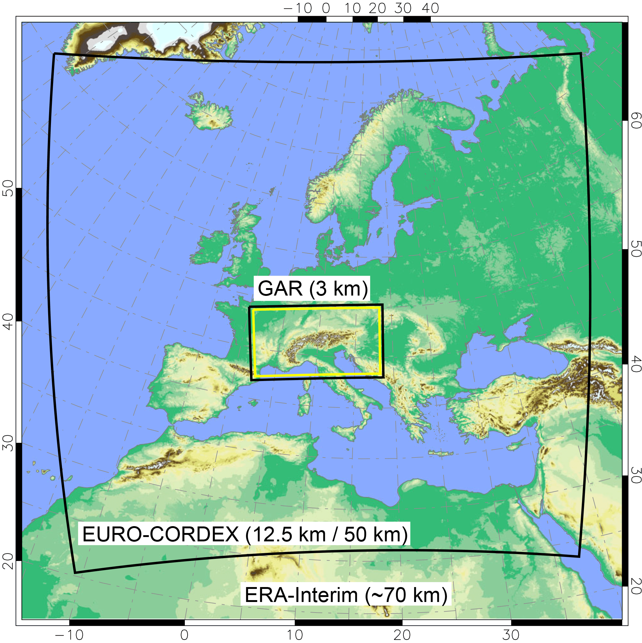
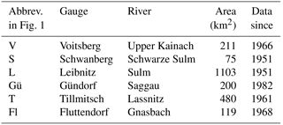
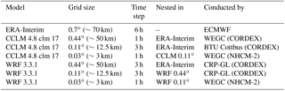
Figure 2RCM domains. ERA-Interim is dynamically downscaled with CCLM and WRF from its initial resolution of ∼70 to 3 km in the Greater Alpine Region (GAR) by making use of an intermediate model domain, the EURO-CORDEX domain with 12.5 and 50 km grid spacing.
In the eastern part (so-called Grabenland creeks) only one gauge (Fluttendorf – Fl) is selected because of the relatively homogeneous climate, geology and soils. The run-off record extends over the whole simulation period and data are assumed very reliable according to the data provider (Hydrographic Service). Geology and soils mainly consist of tertiary material. Influence of continental climate is increasing towards the east with values of annual precipitation in the order of annual evapotranspiration: mean annual precipitation (MAP) is 700 mm in the east, whereas in the western part MAP ranges from 1100 mm at the foot to 1500 at the high altitudes.
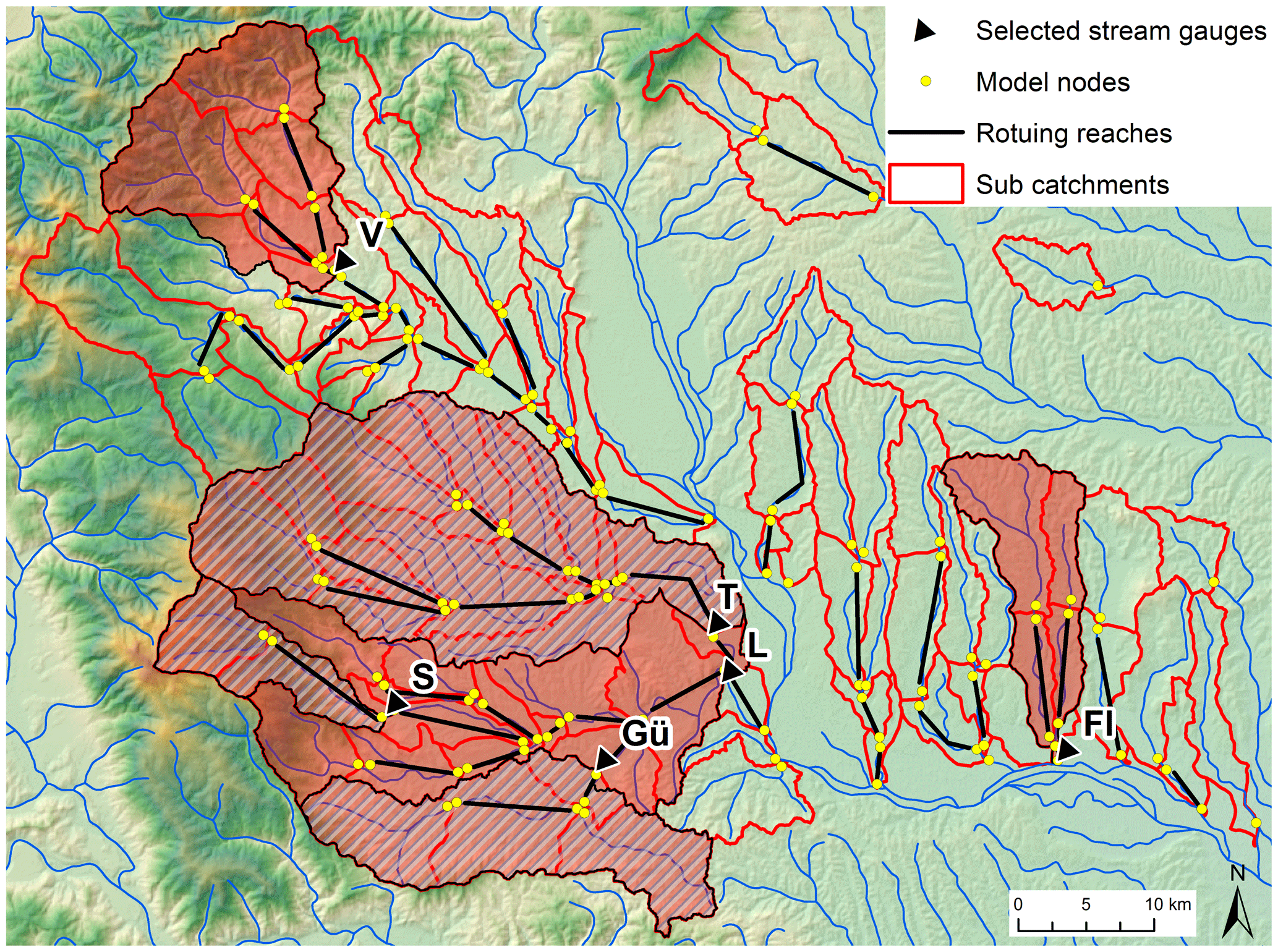
Figure 3Spatial model structure (sub-catchments, nodes, routing reaches), available gauges for calibration and catchments of stream gauges for evaluation highlighted (nested catchments are shaded). Evaluation gauges see Table 1.
3.1 Regional climate models
The RCMs we employ are the non-hydrostatic Consortium for Small-scale Modeling (COSMO) model in CLimate Mode (COSMO-CLM or CCLM) (Böhm et al., 2006; Rockel et al., 2008) version 4.8 clm 17 and the Advanced Research version of the Weather Research and Forecasting Model (WRF/ARW) (Skamarock et al., 2007) version 3.3.1. Both models are driven by the reanalysis data set ERA-Interim (Dee et al., 2011) and cover the period 1989 to 2010. The models' innermost domain, the Greater Alpine Region (GAR) with 3 km grid spacing, is reached via intermediate pan-European domains (without nudging) with 12.5 km grid spacing for CCLM and 50 and 12.5 km grid spacing for WRF. By doing so, we mimic a typical set-up as it is used in regional climate modelling applications and we do not run the risk of underestimating internal variability in our investigations. The simulations of the pan-European domains have contributed to the EURO-CORDEX initiative and have been evaluated in several studies, e.g. Katragkou et al. (2015), Kotlarski et al. (2014) and Prein et al. (2016). The model configurations for the convection-permitting (3 km grid spacing) simulations in the GAR are based on experiences from previous sensitivity experiments (Suklitsch et al., 2011; Awan et al., 2011; Prein et al., 2013, 2015). Our RCMs differ from their coarser resolved counterparts (EURO-CORDEX) insofar that the parameterisation for deep convection, the Tiedtke scheme (Tiedtke, 1989) in CCLM and the Kain-Fritsch scheme (Kain, 2004) in WRF has been turned off in the GAR. Overview of the model domains and simulations used are given in Fig. 2 and Table 2, respectively.
3.2 Error correction
The novel method scaled distribution mapping (SDM) is used to bias correct the model precipitation and temperature data time series (Switanek et al., 2017). SDM is a parametric method, but it is nearly identical to that of quantile mapping (QM) when correcting the historical period. However, for a future period (or any period outside of calibration), the method scales the observed distribution by the relative (for precipitation) or absolute (for temperature) distances between the future and historical modelled cumulative distribution functions (CDFs). The commonly used bias-correction method of QM (Wood et al., 2004; Piani et al., 2010; Themeßl et al., 2011; Teutschbein and Seibert, 2013) assumes that error-correction functions can be treated as stationary from one time period to another. This assumption is responsible for altering the projected climate change signal. For example, a projected mean increase in precipitation of 20 % can be inflated to be 30 %, while extremes can be altered even more dramatically. However, Maraun (2012), Teutschbein and Seibert (2013), Maurer and Pierce (2014) and Switanek et al. (2017) showed this assumption of a stationary error-correction function to be invalid, and as a result, the altering of the raw-model-projected changes to precipitation and temperature was found to be unjustified. In addition, quantile mapping was found to overestimate values of low precipitation and underestimate high precipitation (Maraun, 2013). SDM, in contrast, does not rely on a stationary error-correction function, but rather attempts to best preserve the raw-model-projected changes across the entire distribution. However, the overestimation (underestimation) of low (high) precipitation intensities remains. Bias correction was performed on RCM precipitation and temperature data independently for each grid cell and calendar month. It was implemented on a 3-hourly window to more accurately capture the observed diurnal cycle.
3.3 Hydrological model
The spatially distributed model KAMPUS (Blöschl et al., 2008) is used, which is in operational use for flood forecasting in Austria. It contains conceptual models for snowmelt, soil moisture accounting and flow routing. The snow model is based on the degree-day approach, which calculates snowmelt depending on the air temperature. For snow accumulation precipitation is split into snow and rainfall by a lower and an upper threshold temperature with a linear transition. Depending on the actual soil moisture, rainfall and snowmelt are non-linearly partitioned into a component that increases soil moisture and a component that contributes to run-off, dQ. Soil moisture can only be depleted by evapotranspiration. Run-off routing on a raster cell (hillslope) is represented by an upper zone and two lower zones, which are formulated as linear reservoirs. dQ is the input into the upper zone. The zone has three outlets: (i) outflow with a low storage coefficient (k1) that represents interflow; (ii) percolation to the lower reservoirs (saturated zone); and (iii) when a defined threshold, L1, is exceeded, outflow with a very low storage coefficient (k0) representing surface or near-surface run-off. The percolation rate into the two lower zones is separated into two components by a factor. Outflow of the lower zones is defined as groundwater flow and deep groundwater flow, respectively. A bypass flow, dQby, routes rainfall and snowmelt directly into the lower storages (macropore flow). Model structure is described in detail in Blöschl et al. (2008). In this work, the original vertical structure is extended by a module for infiltration excess. At very high intensities (I>Icrit) parameters of soil storage are reduced, and bypass and deep percolation is set to zero. Values for Icrit and the reduction of infiltration parameters are obtained by calibration.
Total run-off on a grid cell is calculated as the sum of the outflows from all zones. It is then aggregated to sub-catchments and convoluted by a linear storage cascade which represents run-off routing in the stream network within each of the sub-catchments. Routing in the river reaches which connect model nodes is formulated by a cascade of linear reservoirs (Reszler et al., 2008b). Using a stepwise linear formulation, this model allows for incorporating non-linear effects in flood rooting, such as flood wave acceleration at high water levels and flood retention at flood plains. For the latter, discharge thresholds for flooding the banks and levees and existing 2-D hydrodynamic studies have been provided by the Hydrographic Service of Styria for calibrating the corresponding parameters. This is particularly important for a plausible representation of flood peak attenuation in very large floods. Since the hydrological model is also driven by simulated, often biased, precipitation input, flood peaks which exceed observations may be simulated.
The model domain extends over all of southern Styria (grey shaded window in Fig. 1). The western part has previously been calibrated (Ruch et al., 2012), as it is implemented for operational flood warning by the provincial government of Styria. The eastern part was extended in the current study. The model has a sub-catchment structure with 96 catchments and 152 internal model nodes (Fig. 3). The model is driven by precipitation and air temperature with an hourly temporal resolution and a 1 km gridded spatial resolution. No further climate variables are required; the potential evaporation is represented by the modified Blaney–Criddle method (Schrödter, 1985), which only requires air temperature as input.
The method of extending the model to the eastern domain followed the strategy outlined by Reszler et al. (2006, 2008a). This approach contains several steps for parameter identification based on the dominant processes concept (e.g. Grayson and Blöschl, 2000) and proposes the usage of auxiliary information and data (e.g. field surveys, snow depths, hydrogeological data) and the stratification into different event types (convective, advective and snowmelt events). Spatially distributed information is incorporated in a GIS framework, but the resulting hydrotope (i.e. areas with similar hydrological behaviour, also called hydrological response units) structure is manually fine tuned. The following hydrotope types were chosen (compare to Reszler et al., 2006): urban areas, low-density urban areas, steep slopes open, steep slopes forest, flat agricultural areas with porous aquifer, saturation areas and karstic areas. Hydrotope structure and parameter values are chosen in consistency with the existing model in western Styria, where in some catchments (e.g. at the foothills of the Koralpe massif) the physiographic situation is similar.
3.4 Evaluation measures
In order to combine quantitative and qualitative evaluation of the different model simulations, the following measures are chosen:
-
catchment size as an indicator for general attenuation effects;
-
frequency of floods, i.e. maximum annual floods (MAF);
-
seasonality of floods;
-
other variables, such as soil moisture (simulated by the hydrological model);
-
event-based analyses (performance at particular events, event/weather types).
Catchment size is implicitly incorporated by the selection of the gauges with a wide range of catchment areas from small to medium scale (75 to 200 km2) as well as the larger catchments of the gauges downstream (<1100 km2) (Table 1). In the evaluation plots in this paper the size is identified by the letters “L” for large, “M” for medium and “S” for small. In addition, differences between the catchments in run-off generation and response times are evaluated by different model parameters obtained by the calibration.
Frequency of floods are analysed by typical statistics of maximum annual flood peaks using the following plotting position (Weibull)
RP is the (empirical) return period, N the number of values (years) and m the ranking (1 for the maximum and N for the minimum flood).
The seasonality of floods gives first insights into the main hydrological drivers for flood occurrence (Parajka et al., 2010). It is the result of the relative influences of soil moisture, evaporation and snow processes and varies considerably in space. In their event-type analyses, Merz and Blöschl (2003) used the seasonality of maximum annual flood peaks as an indicator describing the timing of floods. Here, seasonality is first analysed simply by counting MAF peaks in the four seasons: December, January and February (DJF); March, April and May (MAM); June, July and August (JJA); and September, October and November (SON). Second, in order to illustrate seasonality for different simulation runs in the small multi-model framework, circular statistics are performed. For each event the date of occurrence of the MAF is transposed to an angle by
where Di denotes the day of the year (Di=1 for 1 January, Di=365 for 31 December). This angle is averaged by the following equations:
where X and Y are the rectangular coordinates of the mean angle θr; and r is the mean vector length, which is a measure of strengths of the seasonality (r=1 if all events occur at the same date). Note that the final resulting mean angle depends on the quadrant of the calculated mean angle.
Using a hydrological model for an evaluation of climate model results also enables the incorporation of other hydrological quantities, which give indications about the performance of the climate model regarding the hydrological conditions. Soil moisture is an important variable to be analysed in terms of non-linearity and threshold processes in flood generation (e.g. Penna et al., 2011). It is continuously calculated by the hydrological model and, hence, can be used as a comparison between the different simulation runs.
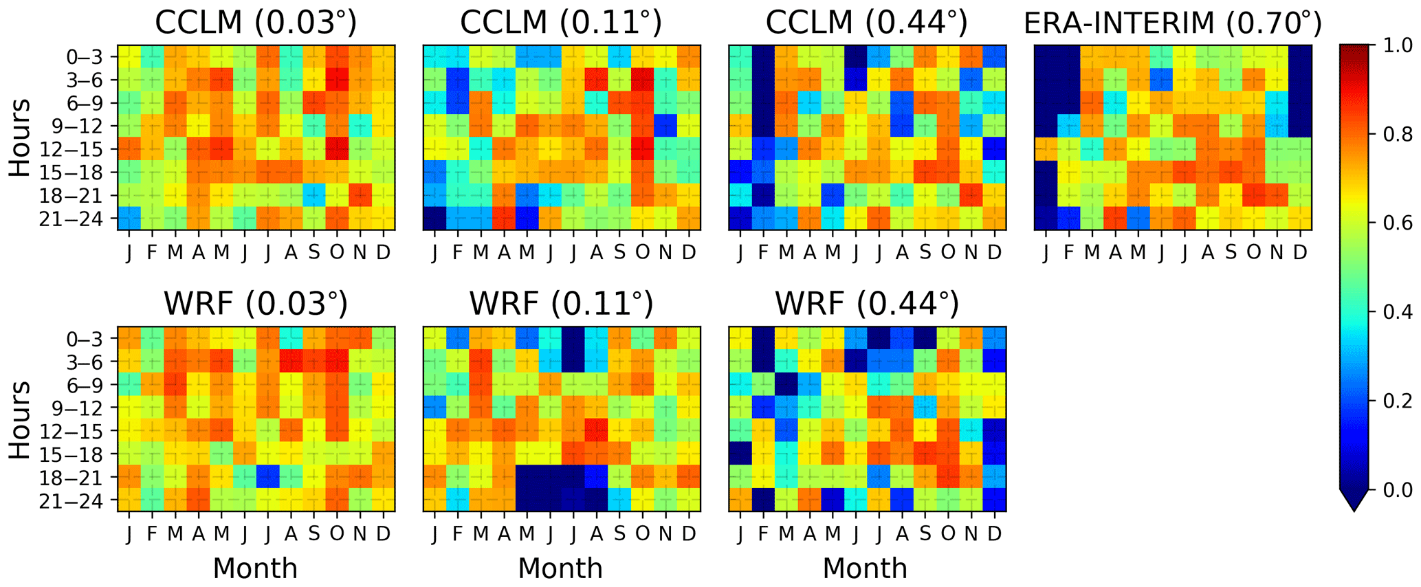
Figure 4Added value of using higher model resolution. The colour bar corresponds to the correlation coefficients between the observed and the modelled spatial fields of averaged precipitation. The x axes and the y axes show the months of the year and the hours of the day, respectively.
At last, mainly using the 3 km convection-permitting RCM results, run-off simulations at characteristic events are checked for their realistic event evolution and the plausibility of the corresponding atmospheric and hydrological conditions.
Table 3Model efficiency at the selected gauges in the calibration and historical (validation) period.
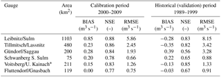
* Continuous run-off data since 1996 (only 4 years in the historical period), but with historical maximum annual flood peaks available (hydrographic year book).
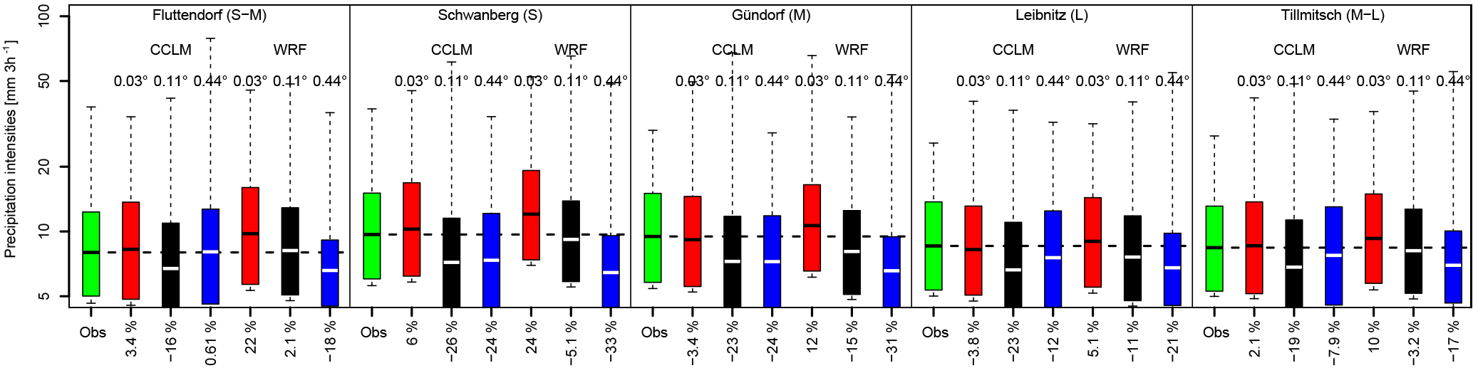
Figure 5Catchment-averaged heavy (>90th percentile) precipitation intensities of observations (green) and CCLM and WRF with 0.03∘ (3 km; red), 0.11∘ (12.5 km; black) and 0.44∘ (50 km; blue) grid spacing. Y axis has a logarithmic scale. Coloured boxes indicate the 10th–90th inter-quantile range, horizontal markers in the boxes denote mean values and whiskers refer to maximum values. Relative biases of mean values are given along the x axis.
In order to demonstrate added value due to a reduction in the model grid spacing, we derived averaged precipitation fields of the models and the observational data and calculated the spatial correlation coefficient between them. Figure 4 illustrates the resultant correlation coefficients for all models, months and hours of the day. Higher correlations for both models, illustrated by the warmer colours, are more clearly observed towards the left side of Fig. 4, the side where highest model resolutions are depicted. This shows that the RCMs improve, on average, in their ability to simulate precipitation fields across space as the resolution of the model increases.
Added value is also seen on catchment-averaged quantities. Generally, the convection-permitting models increase precipitation intensities from heavy (>90th percentile) precipitation events in all catchments. In the case of CCLM, this results in added value (together with some overestimation), since the coarser resolved counterpart CCLM 0.11∘ largely underestimates (in the range of −16 % to −26 % across the catchments) precipitation intensities on average (see Fig. 5). In contrast, WRF does not show such strong underestimations in the 0.11∘ simulation and WRF 0.03∘ gives an overestimation, because of its linkage to the coarser resolved 0.11∘ simulation that enables error propagation (Addor et al., 2016). The reasons for the enhancement of intensities in mountainous regions may be a result of the higher resolved orography, which is in agreement with previous evaluation studies (Knist et al., 2018; Prein et al., 2013; Ban et al., 2014; Langhans et al., 2013). Note that WRF 0.11∘ is generally in a better agreement with the observations than CCLM 0.11∘ (Fig. 5), although both simulations are of comparable performance on the European domain (e.g. Katragkou et al., 2015; Kotlarski et al., 2014) and add value in mountainous regions compared to their 0.44∘ counterparts (Prein et al., 2016).
The hydrological model was calibrated, for each sub-catchment, against run-off data of all available stream gauges in the period 2000–2009 (Fig. 1). Calibration results in western Styria are available, and the found parameters in catchments with similar soil and geological properties serve as a priori values for the catchments in the extended part. The historical data in the current study (1989–1999) are used for model validation. This allows also a validation of the existing model; these data were provided for the current study and had not been used for model calibration. Quantitative metrics such as the commonly used Nash–Sutcliffe efficiency (NSE, Nash and Sutcliffe, 1970), the bias based on mean run-off values and the root mean square error (RMSE) are used to measure model calibration. In Table 3 the results for the selected gauges are listed. As it is often the case, NSE is lowest in the smaller catchments, e.g. Schwanberg and Fluttendorf with 0.77 and 0.78 in the calibration period, respectively. In the validation period the NSE falls below 0.7 in these two catchments. The historical period also includes phases with poor data availability (see Fig. 1), which is also the reason for the drop in the NSE value in the validation period at the Gündorf gauge.
Examples of hydrographs in the calibration and validation period are attached in the Supplement (Figs. S1 and S2). In addition to flood peaks, run-off generation and rainfall response is represented very well. Differences in the shape of hydrographs are also accurately simulated. For example, the Schwanberg gauge shows short peaks due to short concentration times in the small catchment but at the same time high baseflow. The latter indicates a high fraction of slowly draining flow components (groundwater) from long-term storage. On the other hand, in the medium-sized Gündorf catchment, short peaks also indicate short response times, but baseflow is significantly lower. This difference can be attributed to the different geologic conditions in the area. In the Schwanberg catchment the significant subsurface storage can be attributed to a deep weathering zone overlaying schists and gneiss, and geology in the Gündorf catchment consists mainly of tertiary material (silt, loam) with very low storage capacities. In the larger catchments flood peaks are smooth, lasting over several hours, which shows the attenuation effects (Tillmitsch, Leibnitz). The resulting model parameter values representing timescales of run-off response show the flashy character in the catchments: The time constant of the fast flow component, i.e. surface run-off in open steep slopes (k0), at the hillslope scale is in the order of simulation time step of 1 h, routing within the sub-catchments (30–50 km2) is in the same order and travel time within most river reaches connecting the nodes is 2–3 h.
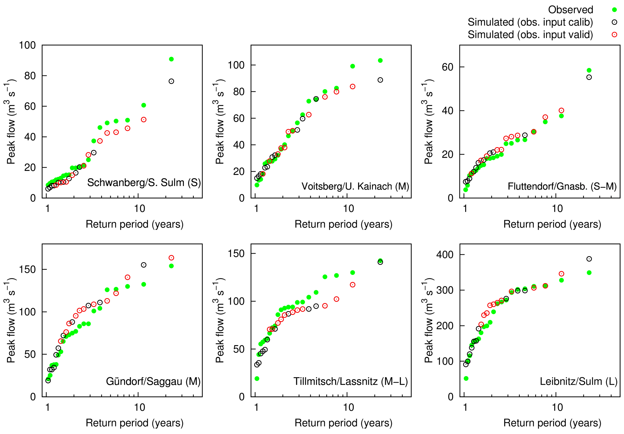
Figure 6Simulated and observed maximum annual flood peaks vs. empirical return periods (Eq. 1, flood frequency plots) of the selected gauges in the period 1989–2010. The peaks in the validation period are marked with red colour.
For this study, representation of flood frequency is important. Model-simulated maximum annual floods for the entire study period (calibration and validation period combined, 1989–2010, 22 years) are compared with observed flood peaks in Fig. 6 (flood frequency plot). Although the MAF distribution was not explicitly subject to calibration, and the data availability was relatively poor in the period 1990-2000, the model accurately simulates observed flood statistics at the selected gauges. The largest flood is simulated well at all gauges, while simulation results at the smaller events are reasonable. Both in the calibration and validation period, deviations in significant events are analysed in terms of probable errors in input (precipitation), model structure, model parameters and/or run-off data. At the exceptional events threshold processes are operative, which are accurately simulated. For example, the largest flood at the Schwanberg gauge in August 2005 (Fig. 6, plot above left, extrapolated RP would be more than 100 years) was a very local event (see Fig. 9 lowest panel) and the interpolated rainfall is assumed to be relatively uncertain. In order to simulate the observed flood peak, parameters which are not plausible and decrease model performance at other large events would be needed. Also inundation occurred during the event in the Schwanberg town, which likely led to uncertainties in the observed peak run-off data. At the Fluttendorf/Gnasbach gauge, flooding occurred at the two events in 2009 (see Fig. 5), and retention by inundation in flood plains was calibrated successfully in the flood routing model. At the Voitsberg gauge the two largest floods were slightly underestimated. The largest flood occurred in October 1993, within the validation period, which was underestimated in the simulation. The largest flood in the simulation is the 2009 flood, which was represented very well (see Supplement). Data quality used to be poor in 1993 in the high-altitude catchment in the north-western part. Station density in this part today is still lower than for example in the south-western part (see Fig. 1). The same situation can be stated for the Tillmitsch gauge. At this gauge, the four medium event peaks (from 92 to 117 m3 s−1) are the MAFs in the years 1993 – 1996, and the simulated flood peaks at the corresponding plotting positions were slightly underestimated.
With the calibrated hydrological model, simulations are performed using the results of the RCMs as input. In Sects. 6.1 and 6.2, evaluation results are discussed in detail for the run-off simulations using the CCLM results. The same procedure has been applied using the WRF results (provided in Supplement). In a synthesis step (Sect. 6.3), all the results of the small multi-model framework are summarised and compared for formulating final conclusions.
6.1 Uncorrected RCM data
Flood frequency plots for the selected gauges using uncorrected CCLM data (and the ERA-Interim data) as input compared to the observations are shown in Fig. 7. The figure illustrates the improvement of the results using the 3 km CCLM data, particularly for the smallest catchment, Schwanberg/S. Sulm, with a size of approximately 75 km2. In this specific region, the convection-permitting simulation seems to be a necessity in order to accurately represent the magnitude of floods. In some larger catchments the simulations with the coarser RCM data already yield reasonable results. As the plotting positions suggest, the statistical properties, mean and standard deviation decrease with increasing grid size. The skewness does not decrease; in Voitsberg and Schwanberg the CCLM 0.11∘ simulation yields a high skewness. At the latter only three events are simulated with peak flows above 20 m3 s−1, whereas the observation reaches a maximum of 90 m3 s−1.

Figure 7Simulated maximum annual flood peaks using raw CCLM data as input and observed maximum annual flood peaks vs. empirical return periods (Eq. 1, flood frequency plots) of the selected gauges in the period 1989–2010.
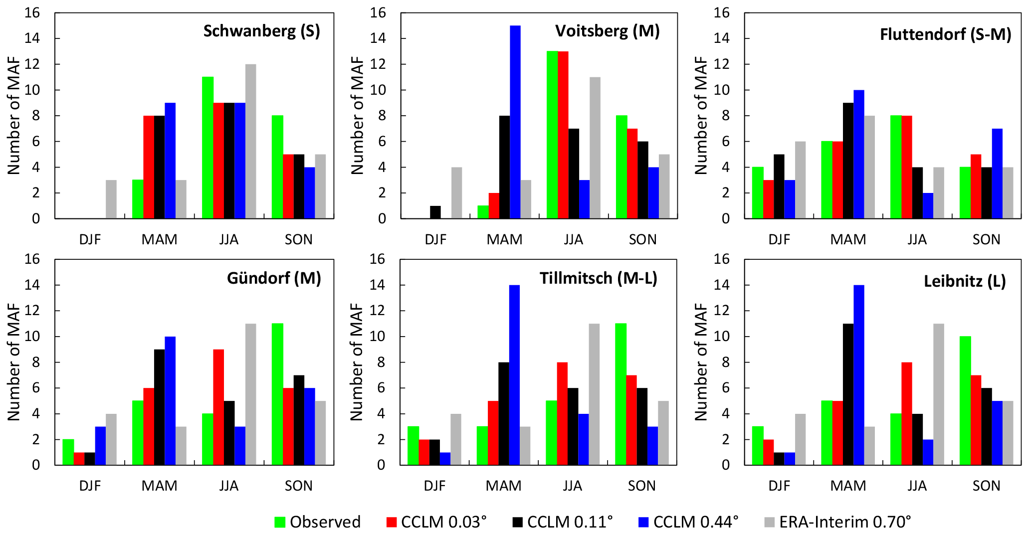
Figure 8Number of maximum annual floods in the four seasons (seasonality) from the simulation using raw CCLM data as input compared to the observation at the selected gauges in the period 1989–2010.
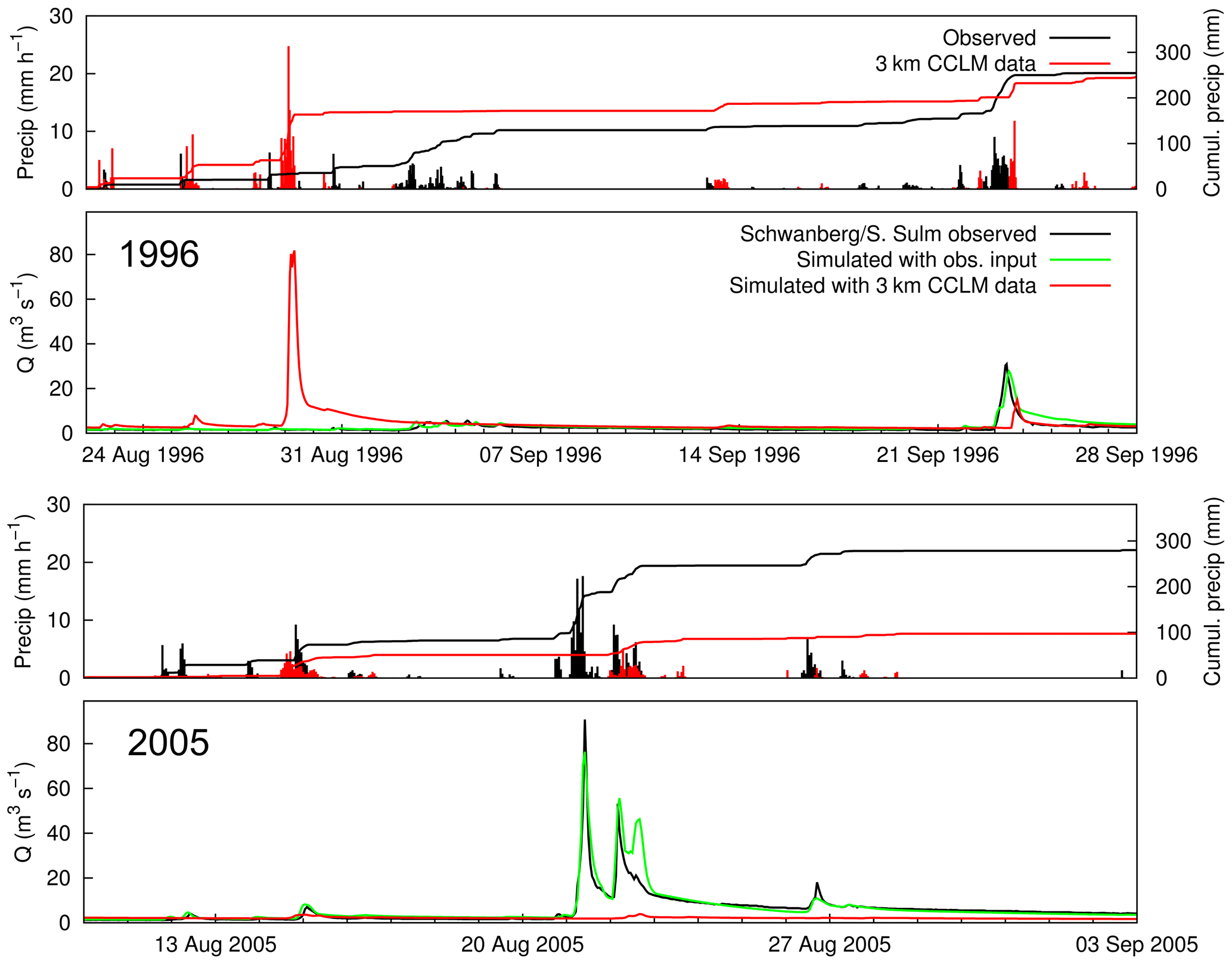
Figure 9Example of two events (August 1996, above, and August 2005, below, in each case plotted with catchment precipitation above the run-off) simulated with raw CCLM 3 km data compared to the simulation with observed input and observed run-off data for the Schwanberg gauge.
Most of the RCM settings show negative biases regarding MAF peaks; however, some are significantly positively biased, e.g. Voitsberg/Kainach in the north-western Alpine part. At the Fluttendorf gauge (upper-right subplot) the 0.44∘ data lead to a maximum flood that significantly exceeds the observations; this peak is the consequence of overestimated heavy rainfall intensities (approximately 300 mm in 18 h), which were simulated in August 2005 during the 2005 European floods (“Alpenhochwasser”). For comparison, the largest observed MAF at the Fluttendorf gauge occurred during an extreme precipitation event in June 2009 (Fig. 15 in the following section).
The seasonal occurrence (winter: DJF, spring: MAM, summer: JJA and autumn: SON) of the simulated MAFs is analysed in Fig. 8. The improvements are evident when reducing grid size; the simulation with the uncorrected 3 km CCLM data represents the observed seasonality very well. The figure further shows that both the CCLM with 0.44∘ (∼50 km) and the CCLM with 0.11∘ (∼12.5 km) grid sizes yield a shift in the flood season from summer (JJA) to spring (MAM) in all catchments – except Schwanberg. Also, in the catchments in western Styria (Kainach, Sulm, Saggau, Lassnitz), the number of MAFs in autumn is underestimated in all CCLM settings. In autumn, frequently occurring low-pressure systems in the Mediterranean or east of the Alpine region induce heavy rainfall which can often lead to large floods (Seibert et al., 2007). The simulations indicate that this is underrepresented in all CCLM data. This shows the value of the use of seasonality for an evaluation of an accurate representation of the main flood-generating mechanisms. Flood statistics in the mentioned cases yielded reasonable results, but this criterion alone could be misleading. In the catchment in eastern Styria (Gnasbach) the relatively uniform distribution is captured well (upper-right subplot). The results for flood frequency and seasonality when using the WRF data are worse than when using the CCLM data (shown in Figs. S3 and S4, and discussed later in Sect. 6.3).
Simulated soil moisture on a monthly basis (attached in Fig. S5 above) shows annual dynamics that are similar to the seasonality of MAF. Also, the improvements using the 3 km CCLM (0.03∘) compared to the coarser resolution are evident, and ERA-Interim is closest to the reference. Within ERA-Interim the observed situation is represented; however, the coarse resolution also leads to a bias. Underestimation in summer is significant, particularly in the case of the 0.44∘ (∼50 km) and 0.11∘ (∼12.5 km) grid sizes. In this season heavy storms occur with often convective character or double events. The corresponding flood magnitude is (non-linearly) controlled by the antecedent soil moisture, which is the consequence of the meteorological and hydrological history prior to the flood events. The same is true for the autumn (SON in Fig. 8), when the soil moisture is underestimated and often floods occur as a consequence of Mediterranean low-pressure systems in combination with wet soils due to reduced evapotranspiration.

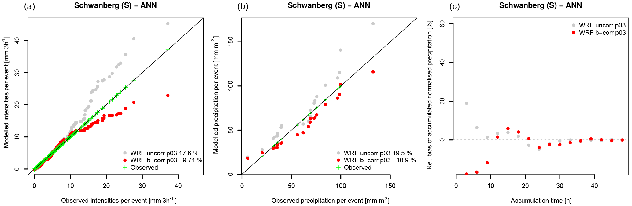
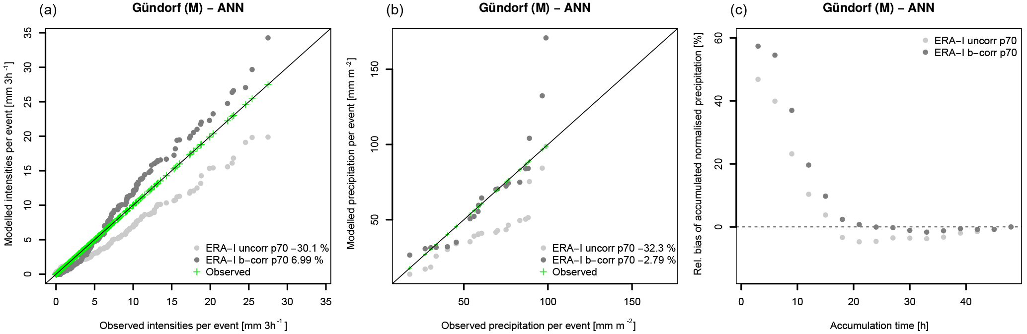
Figure 10Comparison between modelled (CCLM 3 km), bias-corrected and observed precipitation characteristics tied to the 22 MAF events in the Schwanberg catchment. (a) shows the single precipitation intensities. (b) depicts the total precipitation per event (defined as the 2-day period before the maximum peak flow). (c) shows the (event averaged) relative bias of the accumulated precipitation amount (normalised by the events' total precipitation) prior to the flood events as a function of its accumulation time. Numbers in the legends give the relative median bias of the plotted data.
As the first results show, the CCLM 3 km setting yields a clear benefit regarding magnitude and frequency of large floods particularly in small catchments. As stated above, the floods of the simulations are not necessarily aligned in time with observations. Figure 9 shows two simulation periods for the Schwanberg/S. Sulm gauge (75 km2). In the panel above, the period of August and September 1996 is plotted, when the largest flood was simulated with the 3 km CCLM input. There are several small rainfall events in the observation but no large flood occurred during this period. The panel below shows the largest flood in the record, which occurred in August 2005 (Alpenhochwasser). This flood was completely missed using the CCLM input. As it happens, the size and the month of occurrence of the two simulated floods is the same. Also, in 1996 the temporal rainfall distribution simulated by the climate model, showing a very high 1 h block embedded into a slight pre- and post-rainfall, leads to a plausible shape of the hydrograph. This example indicates that large floods are “produced” also for small catchments, which leads to a rather good statistical representation of maximum annual flood peaks (see Fig. 6), but an event-by-event comparison partly fails, because of the large RCM domain: the 3 km CCLM simulation is driven by a 12.5 km CCLM simulation covering the European domain that is in turn driven by reanalysis data (ERA-Interim) without nudging. Due to the internal model variability, the 12.5 km simulation partly deviates from ERA-Interim and even synoptically forced events (like the 2005 flood) may not be correctly represented in space and time in the RCM. This decoupling effect is well known in regional climate modelling and numerical weather prediction and was first published by Kida et al. (1991). Along the modelling chain, the convection-permitting 3 km simulation is affected by decoupling for two times: (1) via the 12.5 km domain that is partly decoupled on the synoptic scale; and (2) via its own internal variability, so that single thunderstorms (under weak synoptic forcing) may occur at different places and/or at different times as in the observations (“double penalty” problem). This limits the applicability of event-by-event comparisons and emphasises statistical evaluation approaches.
6.2 Bias-corrected RCM data
In the same way as for the raw RCM data, the hydrological model is driven using bias-corrected data. After bias correction, results of flood statistics using CCLM (Fig. 13) are improved, except for the smallest catchment, Schwanberg. Here in particular, the results deteriorate compared to the run using the uncorrected data (Fig. 6).
This can be explained by an interference of the temporal distribution of precipitation intensities during the flood-generating rainfall events and the bias correction that simply ignores such temporal relationships. Figure 10 shows the precipitation intensities that contribute to the maximum annual flood events in Schwanberg simulated by CCLM 3 km, before and after bias correction. Each event is limited to a duration of 2 days before the maximum peak flow is reached. Figure 10a demonstrates the work of the bias correction that removes severe underestimation (overestimation) of low (high) intensities in the CCLM 3 km data, but leaves the total amount of precipitation of these events largely unaffected so that a median underestimation of −15 % to −16 % remains (Fig. 10b). The success of CCLM 3 km in capturing the flood events (Fig. 13) lies in the precipitation amount that is accumulated over a shorter time period prior to the flood events. Figure 10c shows the averaged relative bias of accumulated precipitation as a function of the accumulation time prior to the event. On average, CCLM 3 km increasingly overestimates the accumulated precipitation as the accumulation time is shortened. The lack of total precipitation is compensated for by the temporal evolution that gives about 20 % more precipitation within a time range of 24 h before the flood event. The bias correction removes these (compensates for) overestimated intensities and the positioning of the peak flows (Fig. 13) rapidly drops. Note that the reason why single intensities are not properly corrected is based on the fact that the bias correction is independently applied on each grid cell. The remaining deviations from the observations (Fig. 10a) result from the aggregation of single grid cells to areas that cover the entire catchment.
In contrast, the positioning of WRF 3 km peak flows in Schwanberg lies above the observations and the bias correction leads to a deterioration (Fig. S3). In this case, WRF 3 km overestimates precipitation intensities across the flood events and the bias correction changes this (due to the aggregation of single grid cells to catchments) into an underestimation (Fig. 11a). This leads to an overestimation (underestimation) of event-related precipitation amounts (Fig. 11b) for the uncorrected (corrected) data. In WRF 3 km the temporal distribution of the intensities is in much better agreement with the observations than in CCLM 3 km (compare Fig. 11c and Fig. 10c). However, since the total amount is overestimated, the peak flows are higher. The bias correction further deteriorates the temporal distribution of the intensities that lie closer to the flood event and together with the underestimation of the total amount this gives a rapid drop in the positioning of the peak flows (Fig. S3). Note that this good representation of the temporal distribution in WRF 3 km is a catchment-specific feature.
Also, in the small catchments, the aggregation to 3 h sums has an influence on the performance. We tested it by using the 3 h sums of the CCLM 3 km and comparing to the 1 h results (not shown). There is a decrease in flood peaks, but the main decrease in performance in the small Schwanberg catchment is due to the error correction explained above.
In some cases bias correction leads to overcompensating for the flood peaks, particularly in the case of the ERA-Interim data. For instance in Gündorf, flood-event-related precipitation intensities and amounts are largely underestimated in ERA-Interim by more than 30 % on average (median) (Fig. 12a and b), but the precipitation amount within a time range of days before the flood event is overestimated by ∼25 % on average (Fig. 12c). However, this overestimation is too small and the peak flows of the corresponding flood events (Fig. 13) stay below the observations. The bias correction overcorrects the catchment-averaged intensities that are larger than ∼7 mm/3 h (Fig. 12a) and leaves smaller intensities undercorrected (as an effect of catchment aggregation), which yields a good representation of the precipitation amounts (Fig. 12b). The overcorrection of higher intensities leads to a further increase in the accumulated precipitation amount of days prior to the flood events and the corresponding positioning of the peak flows (Fig. 13) lies above the observations in general.
From a return period of 6–10 years the flood simulations are very sensitive to overestimations (e.g. Voitsberg and Gündorf gauges in Fig. 13) and underestimations (see Fig. 7) of the simulated rainfall, which is due to the non-linearity in the rainfall-run-off process (e.g. Komma et al., 2007; Rogger et al., 2012). This threshold is consistent with usual concepts in hydrology, such as the concept of the GRADEX method (e.g. Merz et al., 1999). At this size of floods the soils have been saturated by a high amount of precipitation and 100 % of the subsequent rainfall comes to run-off. This is vital to take into account when it comes to correcting high rainfall intensities within the bias-correction procedure.
Seasonal occurrence is improved for all CCLM settings after bias correction (Fig. 14). In particular, the shift from summer to spring using the raw 0.11 and 0.44∘ data is removed. Again, the 3 km data yield results closest to the observed distribution. Again, results using the bias-corrected WRF data as input are incorporated into discussion in the synthesis step in the following section.
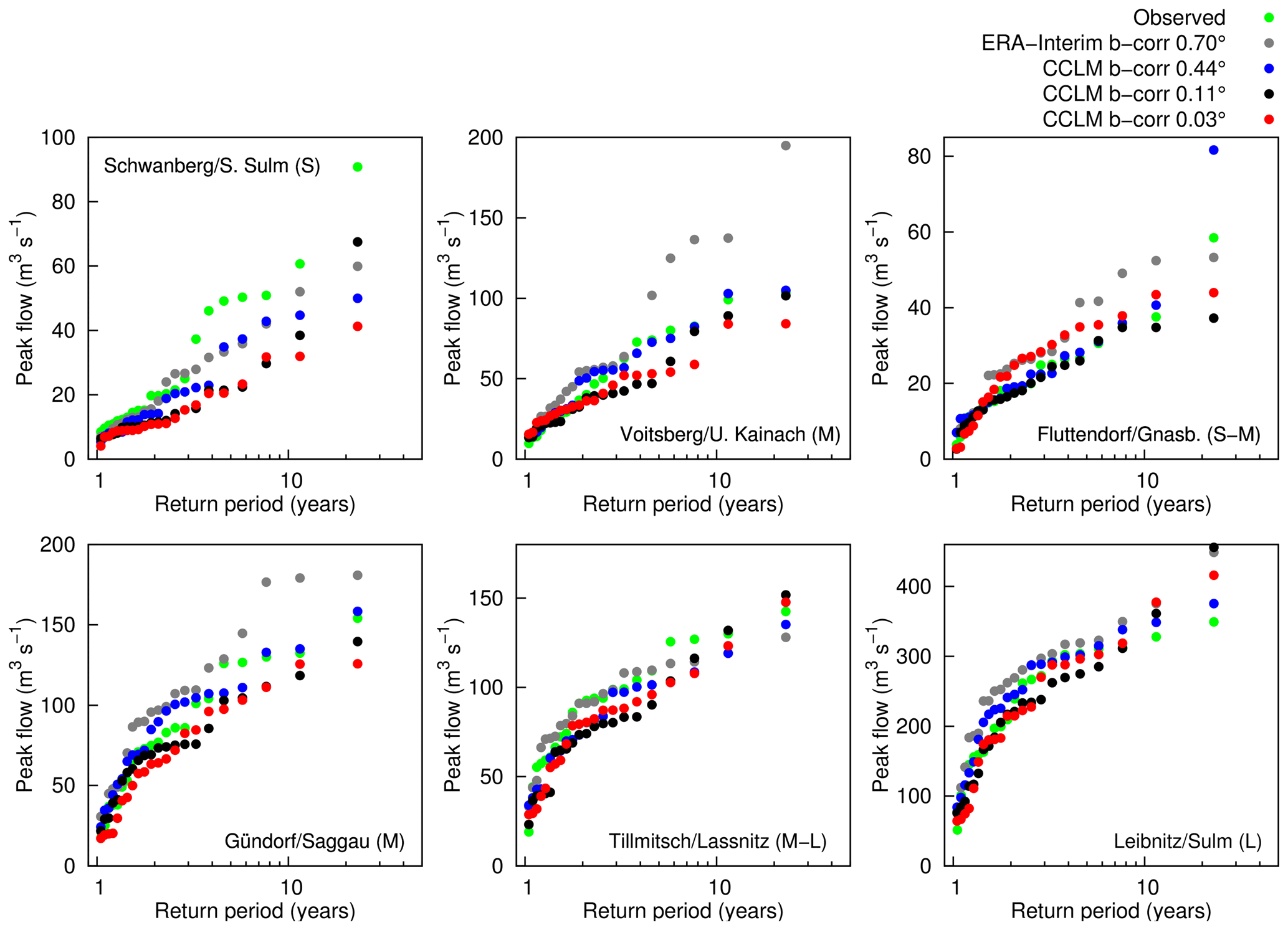
Figure 13Simulated maximum annual flood peaks using bias-corrected CCLM data as input and observed maximum annual flood peaks vs. empirical return periods (Eq. 1, flood frequency plots) of the selected gauges in the period 1989–2010.

Figure 14Number of maximum annual floods in the four seasons (seasonality) from the simulation using bias-corrected CCLM data as input compared to the observation at the selected gauges in the period 1989–2010.
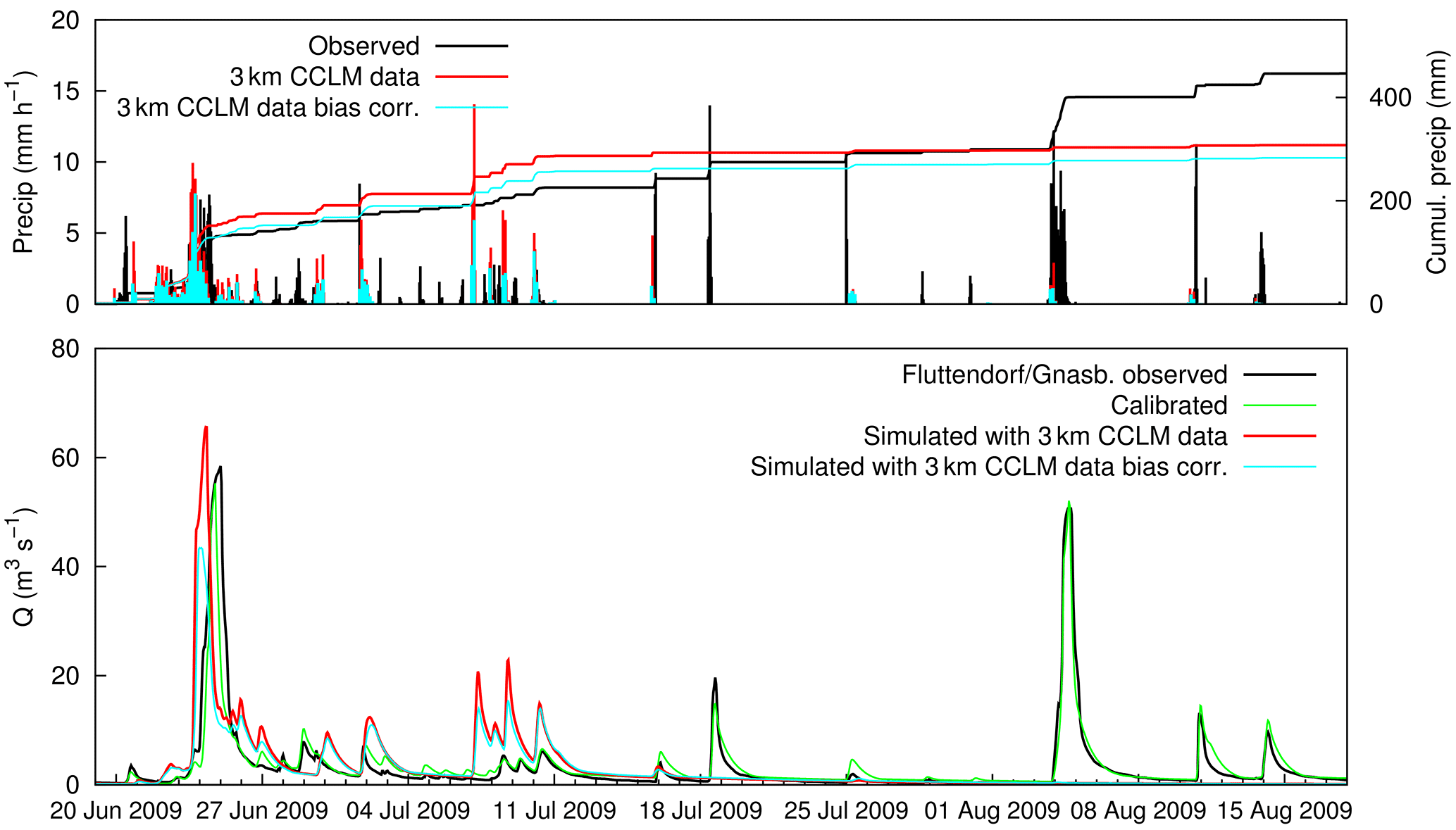
Figure 15Run-off simulated with the uncorrected (1 h rainfall sums) and bias-corrected (3 h rainfall sums) 3 km CCLM data for the period with the largest floods at the Fluttendorf/Gnasbach gauge. Above: catchment precipitation.
As for the seasonality, the seasonal shift in the simulated soil moisture is removed after bias correction, but the underestimation in summer and autumn cannot be entirely compensated for (see Fig. S5 below). This can be attributed to the fact that the modelled events are different in size, shape and overall structure to those of observations. The SDM methodology is performed independently for each grid cell and as a result is not imposing the structure of typical broad-scale observed weather events. Therefore, even though the distributions of bias-corrected precipitation align to observations at individual grid cells, the average precipitation amounts across multiple grid cells can differ from observations. ERA-Interim results now lie exactly on the observation. However, for the MAF performance using ERA-Interim data is not sufficient (compare Fig. 13). This shows that using observed atmospheric conditions with large grid size (∼70 km) is able to reproduce mean monthly hydrological conditions, but fails in flood event representation on this scale. Out of the CCLM data, performance using the 3 km data is still the best, and underestimation using the 0.11 and 0.44∘ data in summer is still evident in all catchments.
For an event-based illustration of the effect of bias correction, two events in 2009 at the Fluttendorf/Gnasbach gauge were chosen using the 3 km CCLM data as input (Fig. 15). The first event in June is the largest in the series and the second event in August is the second largest in the series. Synoptic forcing is different between the two events: the first event is controlled by a persistent upper-air cut-off low that is located over the Balkan region and brings warm and moist air towards the eastern Alpine region from the east (Godina and Müller, 2009). This led to floods in the whole southern Styria region, whereas the second flood is mainly driven by convective processes and concentrated on the eastern part. For the first event, the model with the uncorrected 3 km CCLM data simulates an event with the same order of magnitude, but slightly different timing, as the observation. After the bias correction, flood peak is decreased due to a general reduction of precipitation in the bias correction in this period. A reduction of rainfall in this period results from the bias correction as a consequence of the overestimation of the MAFs by raw CCLM data (compare Fig. 7, upper-right subplot). However, after bias correction, this is still the largest flood peak in the series (see Fig. 13, upper-right subplot). The second event is completely missed by the simulation run with the raw climate model data. No significant rainfall is simulated in the RCM and, hence, bias correction is totally ineffective. It is clear that at such missed events there is no possibility to correct raw RCM data using any statistical bias-correction method. Bias correction is not able to compensate for general uncertainties in representing convective situations. Note that bias-corrected intensities in the upper panel are aggregated 3 h sums.
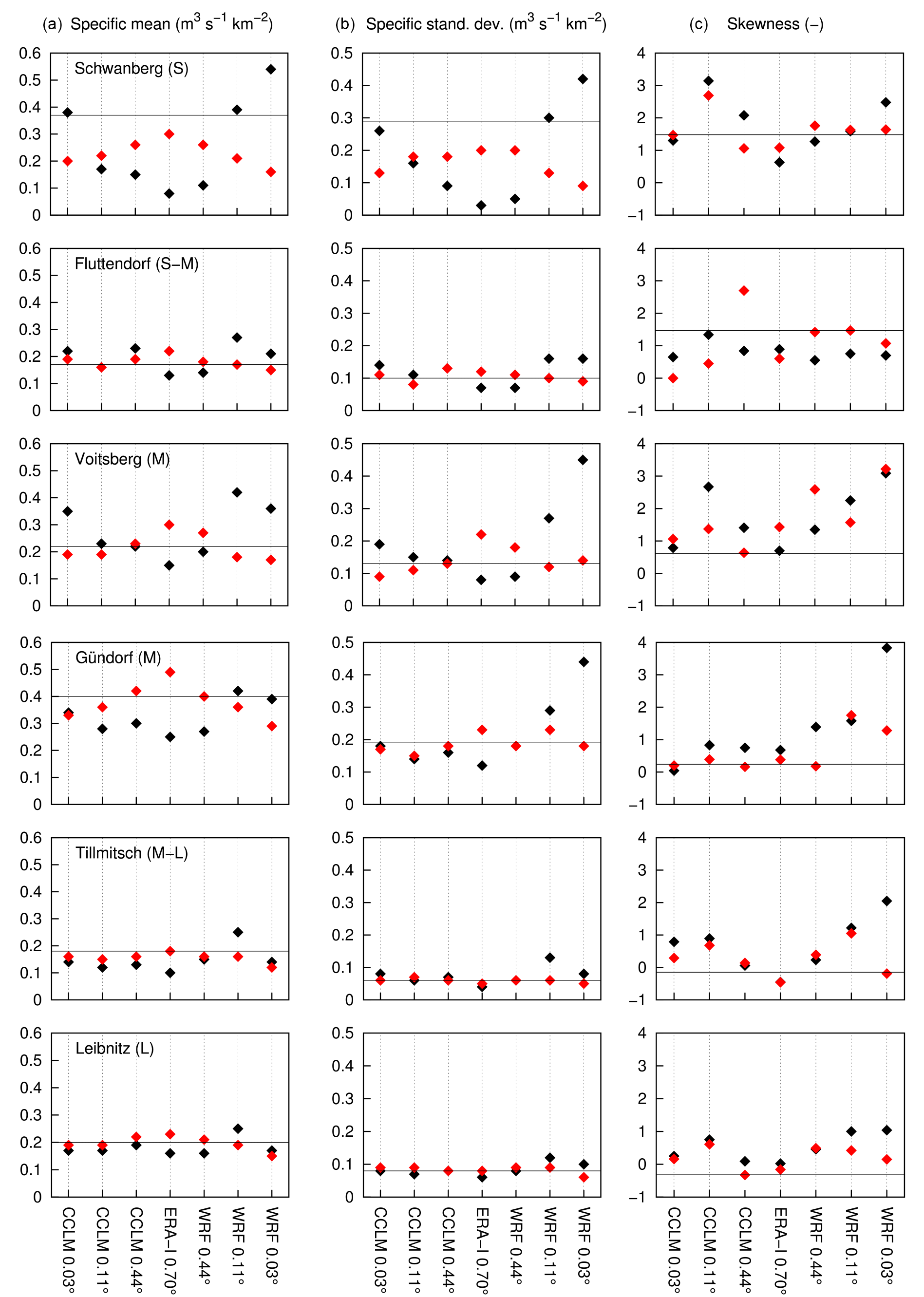
Figure 16Statistical measures of maximum annual flood peak distribution evolving the different model runs. (a) Specific mean, (b) specific standard deviation and (c) skewness. Black: raw RCM data; red: bias-corrected RCM data as input. Black horizontal line denotes the values from the observed flood peak series.
6.3 Synthesis
The statistical measures of mean, standard deviation and skewness for the 22-year sample of maximum annual floods resulting from the 14 different variants are illustrated in Fig. 16. The mean (left plot column) and the standard deviation (middle plot column) are related to the catchment area in order to compare these measures between the gauges. Results using the ERA-Interim data are plotted in the centre, and the results using the different RCM settings with decreasing grid size are plotted towards the left (CCLM) and the right (WRF). The values with raw RCM data as input are plotted as black points; the values with bias-corrected RCM data as an input are plotted as red points. The observed measures are indicated with a thin horizontal line for each gauge. The figure first clearly shows the decrease in mean-specific run-off peaks and – in connection to this – the specific standard deviation with the catchment sizes (S to L from above) for all variants. This is mainly the consequence of a decrease in mean areal precipitation for large rainfall intensities and short durations (e.g. Hershfield, 1961; Lorenz and Skoda, 2000) but also of attenuation effects through flood routing. As discussed in the previous section, in most of the CCLM data-driven simulations the statistical properties are improved reducing the grid size (black points) and further improved after bias correction (red points). For the larger catchments, Tillmitsch and Leibnitz, the differences between the model variants are small, which, again, indicates the good performance of the coarser RCMs regarding general flood statistics (particularly CCLM). This improvement is not always the case for the WRF-driven runs. Particularly large biases from the uncorrected run are either not compensated for (e.g. WRF 0.44∘ for Schwanberg) or even overcompensated for after bias correction (e.g. WRF 0.03∘ for Schwanberg and Voitsberg). The 3 km WRF produces in some periods unrealistic high rainfall intensities over several time steps, which leads to exceptional high flood peaks in the simulation. Examples are the very high values for the skewness (right plot column) at the Gündorf and Voitsberg gauge. This high skewness could sometimes not be compensated for after bias correction, e.g. Voitsberg gauge.
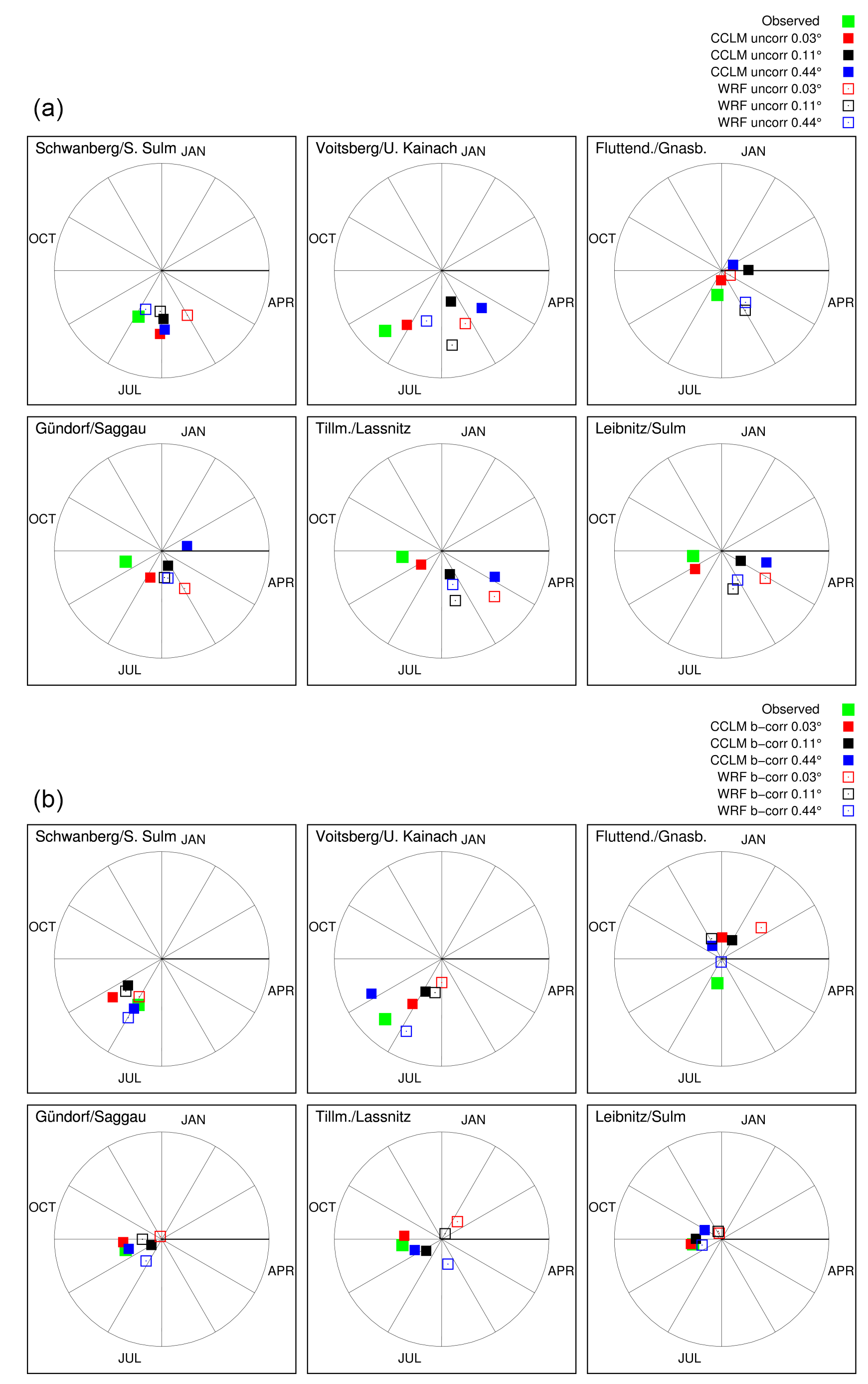
Figure 17Results of seasonality (circular statistics of the maximum annual floods) evolving the different model runs. (a) Raw RCM data as input; (b) bias-corrected RCM data as input. The distance from the centre is the mean vector r and a measure for the seasonality strength, i.e. concentration of timing.
In order to summarise the performance of the small multi-model framework regarding seasonality, Fig. 17 shows the results applying Eq. (2) and Eqs. (3)–(6) on the simulated MAFs using the different RCM data, raw (above) and after bias correction (below). The observation is plotted with a green filled square. As discussed in Sect. 6.1, the results illustrate again the improvement of the seasonality using the 3 km CCLM data (full red squares) compared to the simulations with the coarser CCLM data for all gauges. For example, the highest concentration of timing, i.e. length of vector, of floods in a year in Voitsberg is represented well by the raw 3 km CCLM (upper middle subplot). However, this outstanding result of CCLM 3 km is the result of compensating for errors: the complex interplay between single precipitation intensities and their temporal distribution during flood-generating rainfall events is not correctly represented (Sect. 6.2). Either the total precipitation amount is properly captured but the temporal distribution is failed or vice versa. This also holds for the other RCM simulations, including WRF 3 km, and ERA-Interim. This figure summarizes again that the bias-correction method is not able to correct displacements in this complex interplay.
Using the coarser RCMs, both the timing and strength of seasonality of MAFs deviate significantly from the observations in all catchments. Moreover, the scatter between the different settings is large. However, to some extent all CCLM settings represent the weak seasonality in the eastern part (Fluttendorf catchment, upper-right subplot). The convection-permitting WRF 3 km setting does not provide any improvements compared to the coarser resolutions. Timing of MAFs tends to be concentrated in May/June for all catchments, whereas flood events occur mainly from July to September. This indicates that more or less all WRF settings fail in representing the general mechanisms for flood generation in this area and at this scale. Mostly, discrepancies can be compensated for by the bias correction in the CCLM case, but not for the WRF case. In some catchments using the WRF 3 km settings, the results are worse after bias correction. For example, at the Fluttendorf gauge (upper-right subplot in Fig. 17 below) the concentration of timing shifts from the beginning of May (with a low strength) to February (with a relatively high strength), a month when flood generation is also influenced by snowmelt processes.
This study implemented regional climate models sequentially coupled with a spatially distributed hydrological model to be used for enhanced flood modelling on small and medium spatial scales (up to approximately 1000 km2) in the Eastern Alps. The work is carried out in a small multi-model (ensemble) framework using two different RCMs (CCLM and WRF) in different grid sizes: ∼50 and ∼12.5 km, including two runs at the convection-permitting scale (∼3 km). Additionally, a novel bias-correction method (i.e. a modified version of quantile mapping) is applied to minimise error propagation throughout the modelling chain. Together with the driving ERA-Interim data (grid size ∼70 km) the ensemble contains 14 model variants.
Evaluations using observed data in a historical period (1989–2010) showed that, in the investigated RCM ensemble, no clear added value of the usage of convection-permitting RCMs for the purpose of flood modelling can be found, although CCLM 3 km outperforms in most flood statistics. This is based on the fact that flood events are the consequence of an interplay between the total precipitation amount per event and the temporal distribution of rainfall intensities on a sub-daily scale. The investigated RCM ensemble is lacking in one and/or the other. The seemingly good CCLM 3 km results in the small catchment lie on an overestimation of the intensities and underestimation of the total rainfall amount. This superposition is not systematic across the catchments. From a statistical perspective, all RCMs with all resolutions are able to produce precipitation rates that may cause floods in the study area. In catchments with an area less than 100 km2 a 1 h time step due to the short response times is favourable but the influence is small. In the larger catchments, the 12.5 and 50 km resolutions already yield satisfying results regarding flood statistics. However, with the coarser grid size the seasonality of floods, i.e. date of occurrence in a year, is not accurately represented. This indicates that some main flood generation mechanisms are not captured with the coarser models. CCLM 3 km improves the seasonality of the maximum annual floods; however, in the light of the discrepancies mentioned above, the reason for this is not clear so far. An accurate representation of seasonality is important also in the light of recent findings by Blöschl et al. (2017) that shifts in the seasonality are the only consistent large-scale climate change signal regarding floods identified so far.
The bias-correction-method scaled distribution mapping is able to systematically reduce biases on a seasonal basis. SDM improves results in magnitude and seasonality of maximum annual floods in all settings except for the small catchment (<100 km2), which has to do with the intensity–rainfall amount interplay mentioned above. The procedure corrects the rainfall amount but cannot correct the temporal dynamics. Also, due to the internal model variability, the RCM simulations partly decouple from their driving data and both synoptically forced and convective events may occur at different places and/or at different times as in the observations. Hence, in a usual climate modelling framework, i.e. long simulation periods and large RCM domain without nudging, an event-by-event analysis is not possible. Since the bias correction does not account for this effect and since it does not account for the number of sequential precipitation events (persistence), it might fail for single events and in weather-type-related approaches. Single events with very large biases – as seen using the WRF results – are overcompensated for; i.e. an overestimation is turned into an underestimation and vice versa. This affects the simulated flood peaks particularly for the higher return periods. The results further showed that the bias-correction method is not able to compensate for deviations in the hydrological conditions, particularly in summer. This has implications on flood generation in summer storms, which are frequent in the study area, and highlights the need for further research regarding modifying rainfall events in this season within the bias correction.
With respect to climate change applications of convection-permitting simulations for flood representation we can conclude that, despite the seemingly good results in the CCLM 3 km setting, attention has to be paid and the testing of the results against historical data is of utmost importance. On the other hand, deep convection parameterisations in coarser resolved standard RCMs have been shown to be a source of deep uncertainty. For instance, Kendon et al. (2014) found significant increases in summertime precipitation in convection-permitting climate simulations in the UK while the coarser resolved counterpart does not show any significant change. Ban et al. (2015) and Berthou et al. (2018) found similar results for short-term extreme precipitation events in the Alpine region and in the Mediterranean. In order to circumvent possibly misguided but far reaching climate change adaptation strategies, either convection-permitting RCMs or proper statistical convection emulators (that are currently discussed in the climate modelling communities) should be used. Coarser models could still be used in larger catchments for rough estimations, but they should not be taken for granted regarding local and/or regional flood change. Also, there is a trade-off in the additional costs of a 3 km simulation and the postulated (small scale) process description as long as the physical representation of such small-scale processes can be substituted by statistical ones. Regarding bias correction, the temporal dynamics of the rainfall have to be analysed; an application of a current error-correction method can be recommended only if RCM errors are found to be systematic.
The used hydrometeorological data can be obtained from the Hydrographic Service of the province of Styria (for free) and from the Central Institute for Meteorology and Geodynamics (ZAMG) (for a charge). They were not stored in a separate study-related platform. CCLM simulations with 0.11∘ grid spacing can be found on the data portals of the Earth System Grid Federation (ESGF); WRF with 0.11 and 0.44∘ grid spacing may be obtained from Klaus Görgen (klaus.goergen@fz-juelich.de), Institute of Bio- and Geosciences (Agrosphere, IBG-3), Research Centre Jülich, Germany; and all other RCM simulations (CCLM 0.44 and 0.03∘ as well as WRF 0.03∘) may be obtained from Heimo Truhetz (heimo.truhetz@uni-graz.at), Wegener Center, University of Graz, Austria.
The supplement related to this article is available online at: https://doi.org/10.5194/nhess-18-2653-2018-supplement.
CR performed the hydrological model simulations, MBS implemented and applied the scaled distribution mapping method, and HT conducted the convection-permitting WRF simulations.
The authors declare that they have no conflict of interest.
The study was funded by the Austrian Climate Research Programme (ACRP
6th call, project number KR13AC6K11102 – CHC-FloodS) by the Austrian Climate and Energy
Fund (KLIEN). Regional climate model output on the EURO-CORDEX domain was
provided by Klaus Keuler (BTU Cottbus, Germany) and Klaus Görgen
(Institute of Bio- and Geosciences, Agrosphere, Research Centre Jülich).
The WRF simulations from Klaus Goergen used in this study were conducted at the
Centre de Recherche Public – Gabriel Lippmann (now the Luxembourg Institute of
Science and Technology) under grant FNR C09/SR/16 (CLIMPACT) from the
Luxembourg National Research Fund. The convection-permitting simulations were
conducted in the course of the project NHCM-2 (nhcm-2.uni-graz.at), funded by
the Austrian Science Fund (FWF, project no. P24758-N29). We also thank
Andreas F. Prein (National Center for Atmospheric Research, USA). He conducted the
convection-permitting CCLM simulation and helped with fruitful comments.
Computational resources were provided by the Jülich Supercomputing Centre (JSC)
and by the Vienna Scientific Cluster (VSC). Additionally, we gratefully
acknowledge the European Centre for Medium-Range Weather Forecasts (ECMWF)
for providing ERA-Interim data. Hydro-meteorological data were provided by
the Hydrographic Service of the province of Styria and the Central Institute
for Meteorology and Geodynamics (ZAMG).
Edited by: Joaquim G. Pinto
Reviewed by: three anonymous referees
Addor, N., Rohrer, M., Furrer, R., and Seibert, J.: Propagation of biases in climate models from the synoptic to the regional scale: Implications for bias adjustment, J. Geophys. Res.-Atmos., 121, 2075–2089, https://doi.org/10.1002/2015JD024040, 2016.
Alfieri, L., Burek, P., Feyen, L., and Forzieri, G.: Global warming increases the frequency of river floods in Europe, Hydrol. Earth Syst. Sci., 19, 2247–2260, https://doi.org/10.5194/hess-19-2247-2015, 2015.
Allan, R. P. and Soden, B. J.: Atmospheric warming and the amplification of precipitation extremes. Science, 321, 1481–1484, https://doi.org/10.1126/science.1160787, 2008.
Allen, M. R. and Ingram, W. J.: Constraints on future changes in climate and the hydrologic cycle, Nature, 419, 224–232, https://doi.org/10.1038/nature01092, 2002.
Awan, N. K., Truhetz, H., and Gobiet, A.: Parameterization-Induced Error Characteristics of MM5 and WRF Operated in Climate Mode over the Alpine Region: An Ensemble-Based Analysis, J. Climate, 24, 3107–3123, https://doi.org/10.1175/2011JCLI3674.1, 2011.
Ban, N., Schmidli, J., and Schaer, C.: Evaluation of the convection-resolving regional climate modeling approach in decade-long simulations, J. Geophys. Res.-Atmos., 119, 7889–7907, https://doi.org/10.1002/2014JD021478, 2014.
Ban, N., Schmidli, J., and Schaer, C.: Heavy precipitation in a changing climate: Does short-term summer precipitation increase faster?, Geophys. Res. Lett., 42, 1165–1172, https://doi.org/10.1002/2014GL062588, 2015.
Berg, P., Moseley, C., and Haerter, J. O.: Strong increase in convective precipitation in response to higher temperatures, Nat. Geosci., 6, 181–185, https://doi.org/10.1038/ngeo1731, 2013.
Berthou, S., Kendon, E. J., Chan, S. C., Ban, N., Leutwyler, D., Schär, C., and Fosser, G.: Pan-European climate at convection-permitting scale: a model intercomparison study, Clim. Dynam., https://doi.org/10.1007/s00382-018-4114-6, in press, 2018.
Blöschl, G., Reszler, C., and Komma, J.: A spatially distributed flash flood forecasting model, Environ. Model. Softw., 23, 464–478, https://doi.org/10.1016/j.envsoft.2007.06.010, 2008.
Blöschl, G., Hall, J., Parajka, J., Perdigão, R. A. P., Merz, B., Arheimer, B., Aronica, G. T., Bilibashi, A., Bonacci, O., Borga, O. M., Canjevac, I., Castellarin, A., Chirico, G., Claps, P., Fiala, K., Frovola, N., Gorbachova, L., Gül, A., Hannaford, J., Harrigan, S., Kiss, A., Kjeldsen, T. R., Kohnová, S., Koskela, J. J., Ledvinka, O., Macdonald, N., Mavrova-Guirguinova, M., Mediero, L., Merz, R., Molnar, P., Montanari, A., Murphy, C., Osuch, M., Ovcharuk, V., Radevski, I., Rogger, M., Salinas, J., Sauquet, E., Šraj, M., Szolgay, J., Viglione, A., Volpi, E., Wilson, D., Zaimi, K., and Zivkovic, N.: Changing climate shifts timing of European floods, Science, 357, 588–590, 2017.
BMLFUW: Hydrologic Atlas Austria, in: chap. 6.2: Hydrogeology, Bundesministerium für Land- und Forstwirtschaft, Umwelt und Wasserwirtschaft (BMLFUW), Sektion Wasser – Abt. Wasserhaushalt, Austrian ministery, 2007.
Böhm, U., Kücken, M., Ahrens, W., Block, A., Hauffe, D., Keuler, K., Rockel, B., and Will, A.: CLM – The Climate Version of LM: Brief Description and Long-Term Applications, COSMO Newsletter, 6, 225–235, 2006.
Chan, S. C., Kendon, E. J., Fowler, H. J., Blenkinsop, S., Ferro, C. A., and Stephenson, D. B.: Does increasing the spatial resolution of a regional climate model improve the simulated daily precipitation?, Clim. Dynam., 41, 1475–1495, https://doi.org/10.1007/s00382-012-1568-9, 2013.
Chan, S. C., Kendon, E. J., Fowler, H. J., Blenkinsop, S., Roberts, N. M., and Ferro, C. A.: The value of high-resolution met office regional climate models in the simulation of multihourly precipitation extremes, J. Climate, 27, 6155–6174, https://doi.org/10.1175/JCLI-D-13-00723.1, 2014.
Chan, S. C., Kendon, E. J., Roberts, N. M., Fowler, H. J., and Blenkinsop, S.: The characteristics of summer sub-hourly rainfall over the southern UK in a high-resolution convective permitting model, Environ. Res. Lett., 11, 094024, https://doi.org/10.1088/1748-9326/11/9/094024, 2016.
Dankers, R., Christensen, O. B., Feyen, L., Kalas, M., and de Roo, A.: Evaluation of very high resolution climate model data for simulating flood hazards in the Upper Danube Basin, J. Hydrol., 347, 319–331, https://doi.org/10.1016/j.jhydrol.2007.09.055, 2007.
Dee, D. P., Uppala, S. M., Simmons, A. J., Berrisford, P., Poli, P., Kobayashi, S., Andrae, U., Balmaseda, M. A., Balsamo, G., Bauer, P., Bechtold, P., Beljaars, A. C. M., van de Berg, L., Bidlot, J., Bormann, N., Delsol, C., Dragani, R., Fuentes, M., Geer, A. J., Haimberger, L., Healy, S. B., Hersbach, H., Holm, E. V., Isaksen, L., Kallberg, P., Koehler, M., Matricardi, M., McNally, A. P., Monge-Sanz, B. M., Morcrette, J.-J., Park, B.-K., Peubey, C., de Rosnay, P., Tavolato, C., Thepaut, J.-N., and Vitart, F.: The ERA-Interim reanalysis: configuration and performance of the data assimilation system, Q. J. Roy. Meteorol. Soc., 137, 553–597, https://doi.org/10.1002/qj.828, 2011.
Flügel H. W. and Neubauer, F.: Geologische Karte der Steiermark 1:200.000, Geologische Bundesanstalt, Wien, 1984.
Fowler, H. J., Blenkinsop, S., and Tebaldi, C.: Linking climate change modelling to impacts studies: recent advances in downscaling techniques for hydrological modelling, Int. J. Climatol., 27, 1547–1578, https://doi.org/10.1002/joc.1556, 2007.
Giorgi, F., Jones, C., and Asrar, G. R.: Addressing climate information needs at the regional level: the CORDEX framework, WMO Bulletin, 58, 175–183, 2009.
Gobiet, A., Kotlarski, S., Beniston, M., Heinrich, G., Rajczak, J., and Stoffel, M.: 21st Century Climate Change in the European Alps – A Review, Sci. Total Environ., 493, 1138–1151, https://doi.org/10.1016/j.scitotenv.2013.07.050, 2014.
Godina, R. and Müller, G.: Das Hochwasser in Österreich vom 22. bis 30 Juni, 2009 – Beschreibung der hydrologischen Situation, Report, Austrian Federal Ministry of Agriculture, Forestry, Environment and Water Management (BMLFUW), Abt. VII/3, Vienna, Austria, 21 pp., 2009.
Grayson, R. and Blöschl, G.: Summary of pattern comparison and concluding remarks, chap. 14, in: Spatial Patterns in Catchment Hydrology: Observations and Modelling, edited by: Grayson, R. and Blöschl, G., Cambridge University Press, Cambridge, UK, 355–367, 2000.
Hanel, M. and Buishand, T. A.: On the value of hourly precipitation extremes in regional climate model simulations, J. Hydrol., 393, 265–273, https://doi.org/10.1016/j.jhydrol.2010.08.024, 2010.
Hennegriff, W., Kolokotronis, V., Weber, H., and Bartels, H.: Klimawandel und Hochwasser – Erkenntnisse und Anpassungsstrategien beim Hochwasserschutz, KA – Abwasser, Abfall, 2006, 8, 2006.
Hershfield, D. M.: Estimating the probable maximum precipitation, J. Hydraul. Div. Am. Soc. Civ. Eng., 87, 99–116, 1961.
Hewitt, C. D. and Griggs, D. J.: Ensembles-Based Predictions of Climate Changes and Their Impacts (ENSEMBLES), Eos Trans. AGU, 85, 566, https://doi.org/10.1029/2004EO520005, 2004.
Jacob, D., Petersen, J., Eggert, B., Alias, A., Christensen, O. B., Bouwer, L. M., Braun, A., Colette, A., Deque, M., Georgievski, G., Georgopoulou, E., Gobiet, A., Menut, L., Nikulin, G., Haensler, A., Hempelmann, N., Jones, C., Keuler, K., Kovats, S., Kroener, N., Kotlarski, S., Kriegsmann, A., Martin, E., van Meijgaard, E., Moseley, C., Pfeifer, S., Preuschmann, S., Radermacher, C., Radtke, K., Rechid, D., Rounsevell, M., Samuelsson, P., Somot, S., Soussana, J.-F., Teichmann, C., Valentini, R., Vautard, R., Weber, B., and Yiou, P.: EURO-CORDEX: new high-resolution climate change projections for European impact research, Reg. Environ. Change, 14, 563–578, https://doi.org/10.1007/s10113-013-0499-2, 2013.
Kain, J. S.: The Kain–Fritsch convective parameterization: An update, J. Appl. Meteorol., 43, 170–181, 2004.
Katragkou, E., Garcia-Diez, M., Vautard, R., Sobolowski, S., Zanis, P., Alexandri, G., Cardoso, R. M., Colette, A., Fernandez, J., Gobiet, A., Goergen, K., Karacostas, T., Knist, S., Mayer, S., Soares, P. M. M., Pytharoulis, I., Tegoulias, I., Tsikerdekis, A., and Jacob, D.: Regional climate hindcast simulations within EURO-CORDEX: evaluation of a WRF multi-physics ensemble, Geosci. Model Dev., 8, 603–618, https://doi.org/10.5194/gmd-8-603-2015, 2015.
Kay, A. L., Rudd, A. C., Davies, H. N., Kendon, E. J., and Jones, R. G.: Use of very high resolution climate model data for hydrological modelling: baseline performance and future flood changes, Climatic Change, 133, 193–208, https://doi.org/10.1007/s10584-015-1455-6, 2015.
Kendon, E. J., Roberts, N. M., Fowler, H. J., Roberts, M. J., Chan, S. C., and Senior, C. A.: Heavier summer downpours with climate change revealed by weather forecast resolution model, Nat. Clim. Change, 4, 570–576, https://doi.org/10.1038/NCLIMATE2258, 2014.
Kida, H., Koide, T., Sasaki, H., and Chiba, M.: A New Approach for Coupling a Limited Area Model to a Gcm for Regional Climate Simulations, J. Meteorol. Soc. Jpn., 69, 723–728, 1991.
Knist, S., Goergen, K., and Simmer, C.: Evaluation and projected changes of precipitation statistics in convection-permitting WRF climate simulations over Central Europe, Clim. Dynam., https://doi.org/10.1007/s00382-018-4147-x, in press, 2018.
Komma, J., Reszler, C., Blöschl, G., and Haiden, T.: Ensemble prediction of floods – catchment non-linearity and forecast probabilities, Nat. Hazards Earth Syst. Sci., 7, 431–444, https://doi.org/10.5194/nhess-7-431-2007, 2007.
Köplin, N., Schädler, B., Viviroli, D., and Weingartner, R.: Seasonality and magnitude of floods in Switzerland under future climate change, Hydrol. Process., 28, 2567–2578, https://doi.org/10.1002/hyp.9757, 2014.
Kotlarski, S., Keuler, K., Christensen, O. B., Colette, A., Deque, M., Gobiet, A., Goergen, K., Jacob, D., Luethi, D., van Meijgaard, E., Nikulin, G., Schaer, C., Teichmann, C., Vautard, R., Warrach-Sagi, K., and Wulfmeyer, V.: Regional climate modeling on European scales: a joint standard evaluation of the EURO-CORDEX RCM ensemble, Geosci. Model Dev., 7, 1297–1333, https://doi.org/10.5194/gmd-7-1297-2014, 2014.
Langhans, W., Schmidli, J., Fuhrer, O., Bieri, S., and Schär, C.: Long-Term Simulations of Thermally Driven Flows and Orographic Convection at Convection-Parameterizing and Cloud-Resolving Resolutions, J. Appl. Meteorol. Clim., 52, 1490–1510, https://doi.org/10.1175/JAMC-D-12-0167.1, 2013.
Lenderink, G. and van Meijgaard E.: Unexpected rise in extreme precipitation caused by a shift in rain type?, Nat. Geosci., 2, 373, https://doi.org/10.1038/ngeo524, 2009.
Lenderink, G., Barbero, R., Loriaux, J. M., and Fowler, H. J.: Super-Clausius–Clapeyron Scaling of Extreme Hourly Convective Precipitation and Its Relation to Large-Scale Atmospheric Conditions, J. Climate, 30, 6037–6052, https://doi.org/10.1175/JCLI-D-16-0808.1, 2017.
Lorenz, P. and Skoda, G.: Bemessungsniederschläge kurzer Dauerstufen mit inadäquaten Daten, Nr. 80, Mitteilungsblatt des Hydrographischen Dienstes in Österreich, Wien, 2000.
Maraun, D.: Nonstationarities of regional climate model biases in European seasonal mean temperature and precipitation sums, Geophys. Res. Lett., 39, L06706, https://doi.org/10.1029/2012GL051210, 2012.
Maraun, D.: Bias Correction, Quantile Mapping, and Downscaling: Revisiting the Inflation Issue, J. Climate, 26, 2137–2143, https://doi.org/10.1175/JCLI-D-12-00821.1, 2013.
Maraun, D., Wetterhall, F., Ireson, A. M., Chandler, R. E., Kendon, E. J., Widmann, M., Brienen, S., Rust, H. W., Sauter, T., Themessl, M., Venema, V. K. C., Chun, K. P., Goodess, C. M., Jones, R. G., Onof, C., Vrac, M., and Thiele-Eich, I.: Precipitation Downscaling Under Climate Change: Recent Developments to Bridge the Gap between Dynamical Models and the End User, Rev. Geophys., 48, RG3003, https://doi.org/10.1029/2009RG000314, 2010.
Maurer, E. P. and Pierce, D. W.: Bias correction can modify climate model simulated precipitation changes without adverse effect on the ensemble mean, Hydrol. Earth Syst. Sci., 18, 915–925, https://doi.org/10.5194/hess-18-915-2014, 2014.
Mearns, L. O., Gutowski, W. J., Jones, R., Leung, R., McGinnis, S., Nunes, A. M. B., and Qian, Y.: A Regional Climate Change Assessment Program for North America, Eos Trans. AGU, 90, 311–312, https://doi.org/10.1029/2009EO360002, 2009.
Meredith, E. P., Maraun, D., Semenov, V. A., and Park, W.: Evidence for added value of convection-permitting models for studying changes in extreme precipitation, J. Geophys. Res.-Atmos., 120, 12500–12513, 2015.
Merz, R. and Blöschl, G.: A process typology of regional floods, Water Resour. Res., 39, 1340, https://doi.org/10.1029/2002WR001952, 2003.
Merz, R., Blöschl, G., und Piock-Ellena, U.: Zur Anwendbarkeit des Gradex-Verfahrens in Österreich (Applicability of the Gradex-Method in Austria), Österreichische Wasser- und Abfallwirtschaft, 51, 291–305, 1999.
Nash, J. E. and Sutcliffe, J. V.: River flow forecasting through conceptual models part I – A discussion of principles, J. Hydrol., 10, 282–290, 1970.
Nissen, K. M. and Ulbrich, U.: Increasing frequencies and changing characteristics of heavy precipitation events threatening infrastructure in Europe under climate change, Nat. Hazards Earth Syst. Sci., 17, 1177-1190, https://doi.org/10.5194/nhess-17-1177-2017, 2017.
Parajka, J., Kohnová, S., Bálint, G., Barbuc, M., Borga, M., Claps, P., Cheval, S., Dumitrescu, A., Gaume, E., Hlavčová, K., Merz, R., Pfaundler, M., Stancalie, G., Szolgay, J., and Blöschl, G.: Seasonal characteristics of flood regimes across the Alpine–Carpathian range, J. Hydrol., 394, 78–89, https://doi.org/10.1016/j.jhydrol.2010.05.015, 2010.
Penna, D., Tromp-van Meerveld, H. J., Gobbi, A., Borga, M., and Dalla Fontana, G.: The influence of soil moisture on threshold runoff generation processes in an alpine headwater catchment, Hydrol. Earth Syst. Sci., 15, 689–702, https://doi.org/10.5194/hess-15-689-2011, 2011.
Piani, C., Haerter, J. O., and Coppola, E.: Statistical bias correction for daily precipitation in regional climate models over Europe, Theor. Appl. Climatol., 99, 187–192, https://doi.org/10.1007/s00704-009-0134-9, 2010.
Prein, A. F., Gobiet, A., Suklitsch, M., Truhetz, H., Awan, N. K., Keuler, K., and Georgievski, G.: Added value of convection permitting seasonal simulations, Clim. Dynam., 41, 2655–2677, https://doi.org/10.1007/s00382-013-1744-6, 2013.
Prein, A. F., Langhans, W., Fosser, G., Ferrone, A., Ban, N., Goergen, K., Keller, M., Toelle, M., Gutjahr, O., Feser, F., Brisson, E., Kollet, S., Schmidli, J., van Lipzig, N. P. M., and Leung, R.:, A review on regional convection-permitting climate modeling: Demonstrations, prospects, and challenges, Rev. Geophys., 53, 323–361, https://doi.org/10.1002/2014RG000475, 2015.
Prein, A. F., Gobiet, A., Truhetz, H., Keuler, K., Goergen, K., Teichmann, C., Maule, C. F., van Meijgaard, E., Deque, M., Nikulin, G., Vautard, R., Colette, A., Kjellström, E., and Jacob, D.: Precipitation in the EURO-CORDEX 0.11∘ and 0.44∘ simulations: high resolution, high benefits?, Clim. Dynam., 46, 383–412, https://doi.org/10.1007/s00382-015-2589-y, 2016.
Prein, A. F., Rasmussen, R. M., Ikeda, K., Liu, C., Clark, M. P., and Holland, G. J.: The future intensification of hourly precipitation extremes, Nat. Clim. Change, 7, 48–52, https://doi.org/10.1038/NCLIMATE3168, 2017.
Reszler, C., Komma, J., Blöschl, G., and Gutknecht, D.: Ein Ansatz zur Identifikation flächendetaillierter Abflussmodelle für die Hochwasservorhersage, Hydrol. Wasserbewirt., 50, 220–232, 2006.
Reszler, C., Komma, J., Blöschl, G., and Gutknecht, D.: Dominante Prozesse und Ereignistypen zur Plausibilisierung flächendetaillierter Niederschlag-Abflussmodelle, Hydrol. Wasserbewirt., 52, 120–131, 2008a.
Reszler, C., Blöschl, G., and Komma, J.: Identifying runoff routing parameters for operational flood forecasting in small to medium sized catchments, Hydrolog. Sci. J., 53, 112–129, https://doi.org/10.1623/hysj.53.1.112, 2008b.
Rockel, B., Will, A., and Hense, A.: Special issue on regional climate modelling with COSMO-CLM (CCLM), Meteorol. Z., 17, 477–485, 2008.
Rogger, M., Pirkl, H., Viglione, A., Komma, J., Kohl, B., Kirnbauer, R., Merz, R., and Blöschl, G.: Step changes in the flood frequency curve: Process controls, Water Resour. Res., 48, W05544, https://doi.org/10.1029/2011WR011187, 2012.
Ruch, C., Reszler, C., Rock, G., and Plieschnegger, M.: Flash Flood Warning System – One Model, Two Methods, Geophys. Res. Abstr., 14, EGU2012-9437, 2012.
Schemm, S., Nisi, L., Martinov, A., Leuenberger, D., and Martius, O.: On the link between cold fronts and hail in Switzerland, Atmos. Sci. Lett., 17, 315–325, https://doi.org/10.1002/asl.660, 2016.
Schrödter, H.: Verdunstung – Anwendungsorientierte Meßverfahren und Bestimmungsmethoden, Springer Verlag, p. 186, 1985.
Seibert, P., Frank, A., and Formayer, H.: Synoptic and regional patterns of heavy precipitation in Austria, Theor. Appl. Climatol., 87, 139–153, https://doi.org/10.1007/s00704-006-0198-8, 2007.
Skamarock, W. C., Klemp, J. B., Dudhia, J., Gill, D. O., Barker, D., Wang, W., and Powers, J.: A description of the advanced research WRF version 2, Tech. Rep., NCAR, National Center for Atmospheric Research, Boulder, Colorado, USA, 2007.
Suklitsch, M., Gobiet, A., Truhetz, H., Awan, N. K., Göttel, H., and Jacob, D.: Error characteristics of high resolution regional climate models over the Alpine area, Clim. Dynam., 37, 377–390, https://doi.org/10.1007/s00382-010-0848-5, 2011.
Switanek, M. B., Troch, P. A., Castro, C. L., Leuprecht, A., Chang, H.-I., Mukherjee, R., and Demaria, E. M. C.: Scaled distribution mapping: a bias correction method that preserves raw climate model projected changes, Hydrol. Earth Syst. Sci., 21, 2649–2666, https://doi.org/10.5194/hess-21-2649-2017, 2017.
Teutschbein, C. and Seibert, J.: Is bias correction of regional climate model (RCM) simulations possible for nonstationary conditions?, Hydrol. Earth Syst. Sci., 17, 5061–5077, https://doi.org/10.5194/hess-17-5061-2013, 2013.
Themeßl M., Gobiet, A., and Leuprecht, A.: Empirical-statistical downscaling and error correction of daily precipitation from regional climate models, Int. J. Climatol., 31, 1530–1544, https://doi.org/10.1002/joc.2168, 2011.
Tiedtke, M.: A comprehensive mass flux scheme for cumulus parameterization in large-scale models, Mon. Weather Rev., 117, 1779–1800, 1989.
Trenberth, K. E., Dai, A., Rasmussen, R. M., and Parsons, D. B.: The changing character of precipitation, B. Am. Meteorol. Soc., 84, 1205–1217, https://doi.org/10.1175/BAMS-84-9-1205, 2003.
Wang, G., Wang, D., Trenberth, K. E., Erfanian, A., Yu, M., Bosilovich, M. G., and Parr, D. T.: The peak structure and future changes of the relationships between extreme precipitation and temperature, Nat. Clim. Change, 7, 268–274, https://doi.org/10.1038/NCLIMATE3239, 2017.
Wood, A. W., Leung, L. R., Sridhar, V., and Lettenmaier, D. P.: Hydrologic implications of dynamical and statistical approaches to downscaling climate model outputs, Climatic Change, 62, 189–216, https://doi.org/10.1023/B:CLIM.0000013685.99609.9e, 2004.
Zittis, G., Bruggeman, A., Camera, C., Hadjinicolaou, P., and Lelieveld, J.: The added value of convection permitting simulations of extreme precipitation events over the eastern Mediterranean, Atmos. Res., 191, 20–33, https://doi.org/10.1016/j.atmosres.2017.03.002, 2017.
- Abstract
- Introduction
- Study area and observation data
- Method
- Added value in RCMs due to increased resolution
- Hydrological model calibration and validation
- Evaluation of simulation results using RCM data as input
- Conclusions
- Data availability
- Author contributions
- Competing interests
- Acknowledgements
- References
- Supplement