Low cost, multiscale and multi-sensor application for flooded area mapping

Flood mapping and estimation of the maximum water depth are essential elements for the first damage evaluation, civil protection intervention planning and detection of areas where remediation is needed.

In this work, we present and discuss a methodology for mapping and quantifying flood severity over floodplains. The proposed methodology considers a multiscale and multi-sensor approach using free or low-cost data and sensors. We applied this method to the November 2016 Piedmont (northwestern Italy) flood. We first mapped the flooded areas at the basin scale using free satellite data from low- to medium-high-resolution from both the SAR (Sentinel-1, COSMO-Skymed) and multispectral sensors (MODIS, Sentinel-2). Using very- and ultra-high-resolution images from the low-cost aerial platform and remotely piloted aerial system, we refined the flooded zone and detected the most damaged sector. The presented method considers both urbanised and non-urbanised areas. Nadiral images have several limitations, in particular in urbanised areas, where the use of terrestrial images solved this limitation. Very- and ultra-high-resolution images were processed with structure from motion (SfM) for the realisation of 3-D models. These data, combined with an available digital terrain model, allowed us to obtain maps of the flooded area, maximum high water area and damaged infrastructures.

1 Introduction

Floods are natural disasters that cause significant damage and casualties (Barredo, 2007).

Mapping and modelling the areas affected by floods is a crucial task for (i) identifying the most critical areas for civil protection actions; (ii) evaluating damage and (iii) performing appropriate urban planning (Amadio et al., 2016). To perform a precise quantification of damage, detailed mapping of flooded areas and a reasonable estimation of the water level and flow velocity are required (Arrighi et al., 2013; Luino et al., 2009; Merz et al., 2010; Kreibich, 2009). Advances in remote sensing and technology have introduced the possibility, in the last few years, of generating rapid maps and models during or within a short time after a flood event (e.g. Copernicus Emergency Management Service (©European Union, 2012–2017)). With satellite remote sensing data, it is possible to map flood effects over vast areas at different spatial and temporal resolutions using multispectral (Brakenridge et al., 2006; Gianinetto et al., 2006; Nigro et al., 2014; Wang et al., 2012; Yan et al., 2015; Rahman and Di, 2017) or Synthetic Aperture Radar (SAR) images (Boni et al., 2016; Mason et al., 2014; Schumann et al., 2015; Refice et al., 2014; Pulvirenti et al., 2011; Clement et al., 2017; Brivio et al., 2002). A good description of the main methodologies that are used to map floods with satellite data has been published by Fayne et al. (2017). Moreover, the increasing availability of free-of-charge satellite data with global coverage (e.g. Sentinel-1 and -2 from ESA, and Landsat and MODIS satellites from NASA) makes analyses of flooded areas with low-cost solutions possible. Flood mapping and damage assessment is also an important issue for European Communities authorities that support projects, such as the Copernicus Emergency Management Service mapping (EMSR) and the European Flood Awareness System (EFAS), which manage the activation procedure to acquire satellite data over the areas affected by a natural hazard. De Moel et al. (2009) and Paprotny et al. (2017) described further details about different experiences of flood mapping in Europe.

In urban areas, remote sensing data are often less efficient for the detection of flooded areas, especially if images acquired during the maximum of the inundation are not available. A partial solution could be the use of Remotely Piloted Aerial Systems (RPAS) (Perks et al., 2016; Feng et al., 2015), which are usually able to acquire ultra-high-resolution images over small areas (Giordan et al., 2018). Quantification of the maximum water level caused by the inundation is a crucial parameter, in particular in urban areas, because it can supply damage estimations and support civil protection operations (Luino et al., 2009; Bignami et al., 2017). Very often, nadiral remote sensed platforms cannot define the level of water, and for this reason, field surveys and ground-based photos are still necessary. A possible solution is the use of models for the estimation of the water depth based on digital terrain model (DTM) or hydraulic models (Bates and De Roo, 2000; Segura-Beltrán et al., 2016), but ground truth validation is needed. Recent development of computer vision applications, such as structure from Motion (SfM) (Snavely, 2008), make this system a possible valid alternative for the creation of a 3-D dataset based on terrestrial or aerial image acquisition systems. These datasets can be useful for defining the water depth of flooded areas. The 3-D models derived from SfM are currently used for geomorphological applications (Westoby et al., 2012) and flood mapping. This second application is often assisted using precise DTM derived from lidar (Smith et al., 2014; Meesuk et al., 2015, Costabile et al., 2015). Particular applications of SfM can be used to make 3-D models of facades and acquire a useful dataset for the identification of marks left by water. The combined use of low-cost systems capable of acquire nadiral images and oblique terrestrial pictures is essential for the definition of water levels and the estimation of damage, especially for flooded areas in an urban environment (Griesbaum et al., 2017).

Finally, geolocated photos and information derived from the internet and social media (Rosser et al., 2017; Fohringer et al., 2015) or by volunteer geographic information (Hung et al., 2016; Schnebele and Cervone, 2013) can be handy for improving the mapping of flooded areas.

In this work, we present a smart multiscale and multiplatform methodology that was developed for the identification and mapping of flooded areas. The methodology has been tested in two areas struck by the flood that occurred in Piedmont (northwestern Italy) in November 2016. The paper presents different case studies that are representative of urban and/or non-urbanised areas.

2 Study areas

The Piedmont (Piemonte) region is located in northwestern Italy, and most of the territory is inside the Po River drainage basin (Fig. 1a). The Alps range surrounds the region from north to southwest with an elevation higher than 4000 m a.s.l. In the southern sector, the Ligurian Alps and Apennine Range have lower elevations (1000–2000 m a.s.l.) and separate Piedmont from the Ligurian Sea. On the eastern side, the basin is open to the Po River plain. This orographic setting tends to amplify the effects of some particular meteorological conditions, such as severe and slow-moving cyclones located to the west of Italy that cause a wet flow from the southeast that is blocked by the Alps. This meteorological configuration causes heavy rainfall, especially in autumn when the warm Ligurian Sea is a source of additional energy and humidity (Buzzi et al., 1998; Pinto et al., 2013). In the last 30 years, four main floods hit this region: September 1993 (Regione Piemonte, 1996), November 1994 (Luino, 1999), October 2000 (Cassardo et al., 2013) and November 2016 (ARPA Piemonte, 2016)

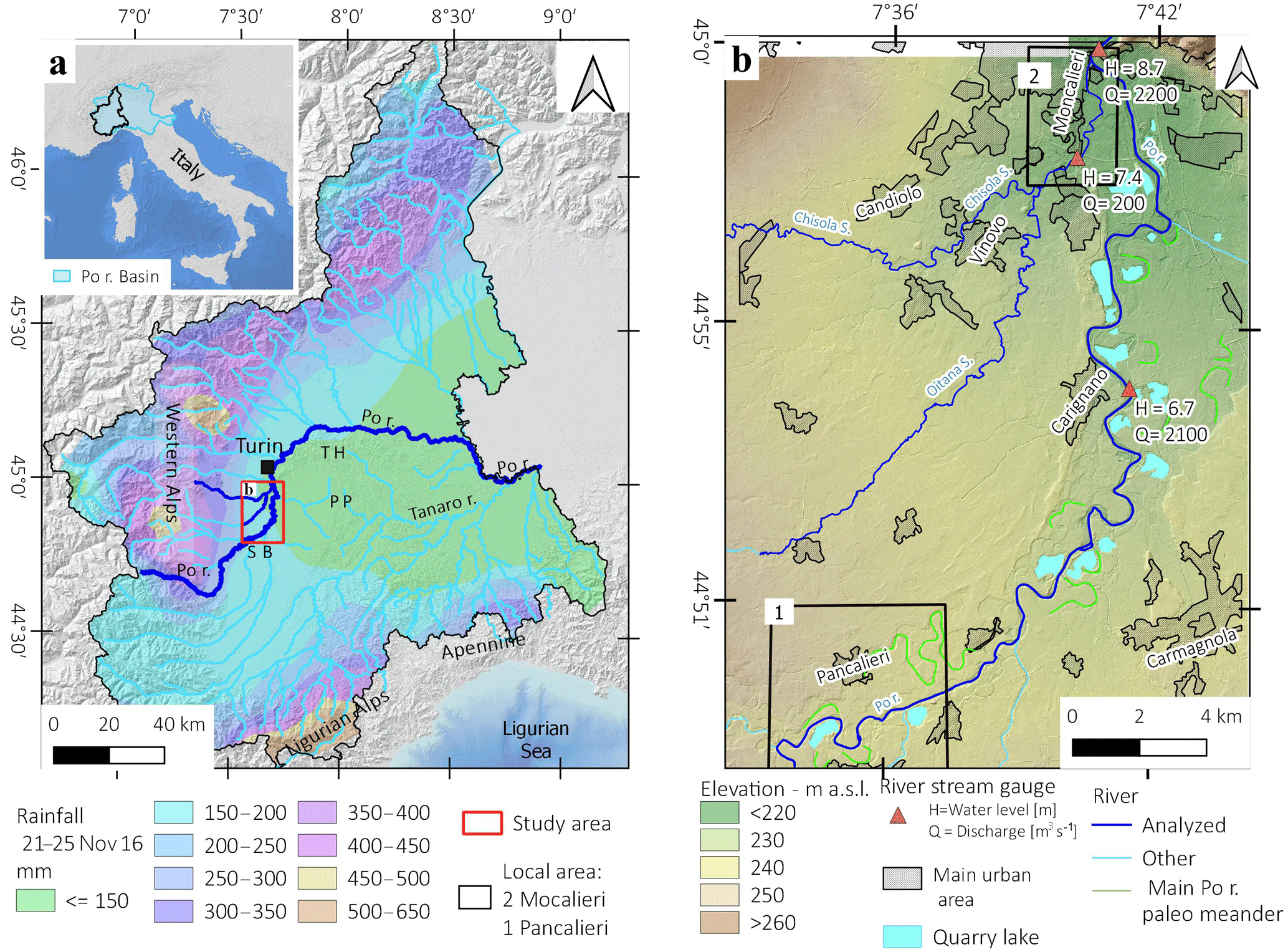
Figure 1 (a) Location of Piedmont region in Italy; (a) rainfall in Piedmont region during the 21–25 November flood event (based on ARPA Piemonte data) and location of study area (SB = Savigliano Basin, PP = Poirino Plateau, TH = Turin Hills) (b) Detailed view of the study area with discharge in the stream gauge stations and the location of Pancalieri (1) and Moncalieri (2) local areas case history.

In November 2016, a severe flood hit the Piedmont region (northwestern Italy). In several areas of the Piedmont in the period 21–25 November 2016, different rain gauges registered an amount of rainfall up to 600 mm, which represented 50 % of the mean annual precipitation (Fig. 1a). The basins of the Po and Tanaro rivers were the most affected by the flood that was very similar, for rainfall distribution and river discharge, to the 1994 event, which is considered one of the most destructive that has occurred in the past decades (Luino, 1999). This time, the event caused large damage, activated numerous landslides and debris flows and caused the inundation of large areas. The civil protection system managed the emergency and the number of victims was sharply reduced compared to the 1994 event that caused 70 victims. The 2016 flood caused a victim in Chisone Valley, not far from Turin.

The presented case study area is located in the Po plain south of Turin (Fig. 1b). This area is mainly occupied by intensive agricultural activity and urban areas primarily located in the northern part. To the south of Turin, many industrial and commercial areas were built in the last decades near the rivers. From the geomorphological point of view, the actual plain (Fig. 1a and b) corresponds to the fill of the Plio–Pleistocenic Savigliano basin (SB), delimited by the western Alps, Turin Hills (TH) and Poirino Plateau (PP). In the western part, it is possible to find alluvial fans of the Chisone, Pellice and Chisola streams (Carraro et al., 1995). The fluvial terraces delimit the actual Po Valley with evident relict geomorphology, such as paleo-meanders. The anthropic influence is remarkable with quarry lakes, revetments and embankments that constrain the riverbeds (Fig. 1b). The geomorphology is a crucial factor that constrains the flooded area shape and the water height.

This area was affected by the flooding of the Po River and other tributaries. In particular, the Chisola and Oitana streams caused severe damage. The Po River between the Carignano and Turin stations reached a maximum discharge of 2000–2200 m³ s⁻¹ in the late evening of 25 November 2016. The mean discharge of this monitoring station in November was 70 m³ s⁻¹. The Chisola Stream registered a discharge of 200 m³ s⁻¹ (November average 17 m³ s⁻¹) near Moncalieri on the afternoon of 25 November (ARPA Piemonte, 2016).

Inside this area (Fig. 1b), we focused our attention in particular on two sites where high-resolution data were acquired:

• The village of Pancalieri, located on the left side of the Po River, just after the confluence with the Pellice River. In this area, it is evident that the ancient Po River meanders are present, and they were reactivated by the flood with damage to some settlements and the destruction of communications roads.

• The town of Moncalieri (approximately 60 000 inhabitants) is located south of Turin in a man-made environment. This area was flooded by Chisola Stream on the late morning of 25 November partly due to the collapse of some sections of the river embankment. The water entered many residential, service and industrial areas with a maximum water height of 1.5–2 m. Another sector of the Moncalieri municipality was also flooded by the Po River in the evening of 25 November, with other damage to commercial and industrial infrastructure.

The activation of Copernicus Emergency Management Service (©2016 European Union) (2016a) EMSR-192 (http://emergency.copernicus.eu/mapping/list-of-components/EMSR192, last access: 23 May 2018) allowed the mapping of the flooded areas (delineation maps) using Radarsat-2, COSMO-Skymed, and Pleiades images in the most critical areas of the Piedmont. In some areas, such as Moncalieri, a map of the damage (grading maps Copernicus Emergency Management, 2016b) was also produced. However, the available delineations maps represent the automatic extraction of the flooded area at the moment of image acquisition, and generally not at the maximum extension. In the case of Piedmont, they cannot be used for exhaustive modelling and damage evaluations. The preliminary estimate of the damage to buildings made by the municipality of Moncalieri was approximately EUR 50 million for industrial buildings and EUR 13 million for residential buildings, and another EUR 6 million for damage to other goods (http://www.comune.moncalieri.to.it/flex/cm/pages/ServeBLOB.php/L/IT/IDPagina/3669, last access: 23 May 2018).

3 Materials and Methods

The aim of this study is the definition of a possible methodology for the identification and mapping of flooded areas using low-cost solutions. For this reason, we have combined and compared data from different sensors. We used different approaches for flood mapping – some have already been tested for a long time as reported in the literature, and others are more innovative and experimental. We first introduce the concept of “co-flood” and “pre- and post-flood” data. Co-flood data are collected around the time of the maximum inundation, while pre/post-flood data are acquired before or after the flood maximum. In the first case, the mapping of flooded areas is more straightforward, but the acquisition of co-flood images was not always possible.

Using a multiscale approach, we developed a methodology (Fig. 2) that progressively considers the use of satellites and then high and ultra-high-resolution systems. The aim is the acquisition of a dataset that can be used to support the identification of the water depth and extent reached by the flood. The dataset also allowed making a first evaluation of damage in both urbanised and non-urbanised areas.

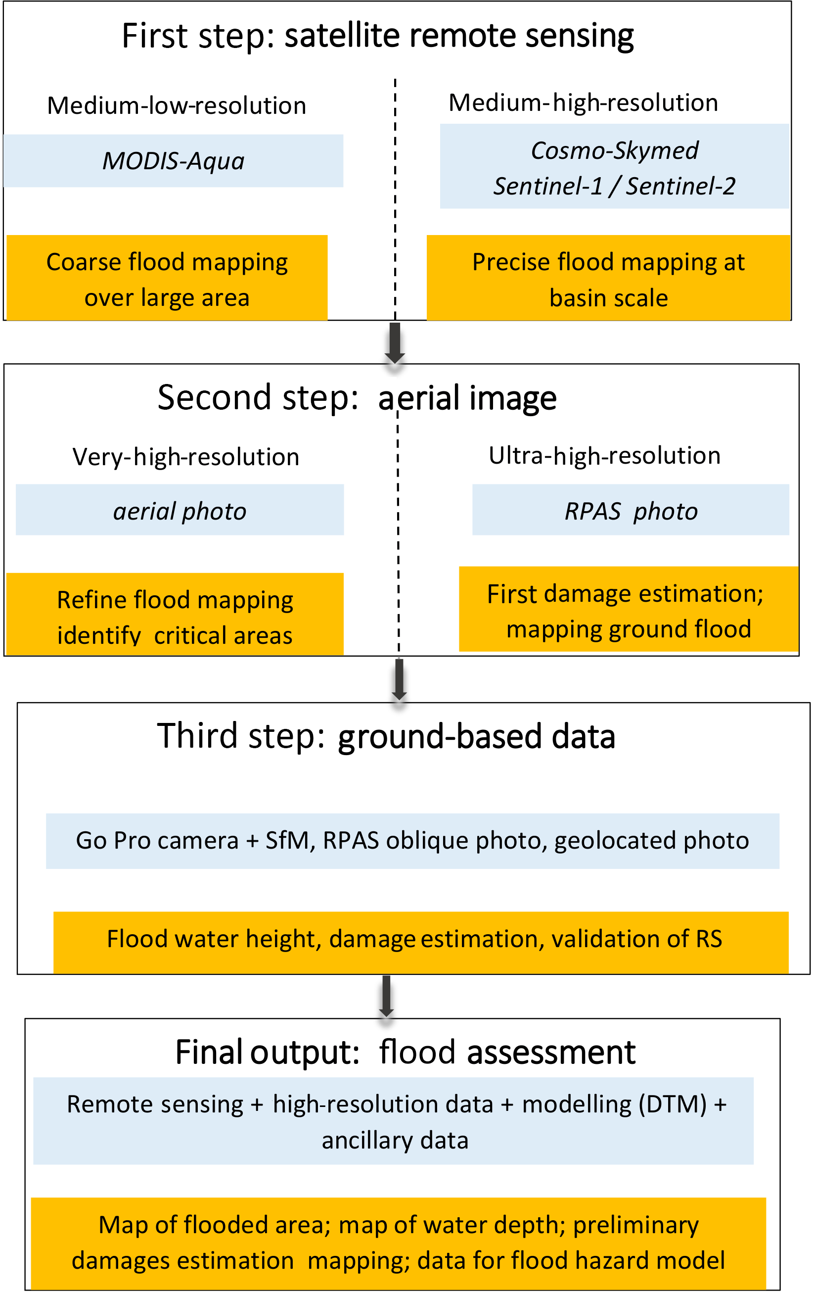
Figure 2 Flowchart illustrating the multiscale flood mapping approaches proposed in this work.

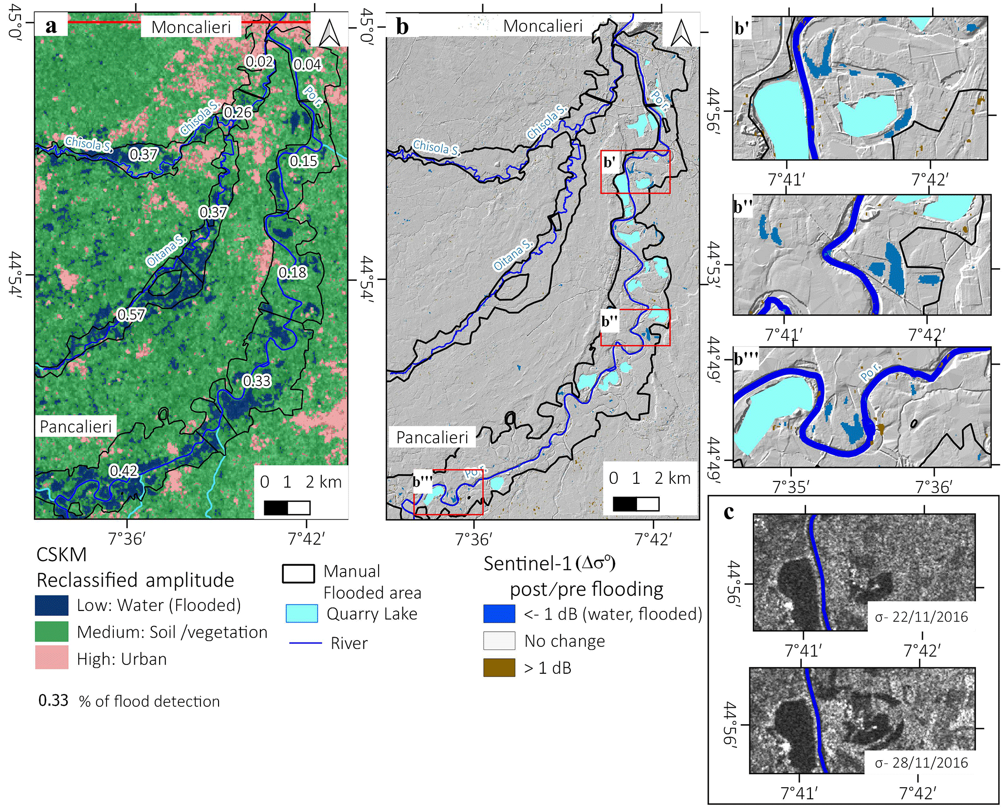
Figure 3 (a) Reclassified Quicklook Amplitude SAR Image acquired at 05:05 UTC, 25 November 2016 – COSMO-SkyMed©ASI [2016]. (b) Sentinel-1 geocoded backscattering coefficient difference (Δσ^∘), (b', b” and b”') and details of some areas where Δσ^∘ still detect water. (c) Example of change backscattering between the pre- and the postflood image is detectable.

The first identification of the flooded area can be made using satellite results and in situ information from the civil protection system that collects reports from local authorities (co-flood phase). This first identification phase is mandatory to have a general and fast indication of the involved area and to plan more detailed acquisitions.

The second phase is aimed at acquiring a high definition dataset that can be used for a detailed mapping of the flooded area. For this step, a system is required that is able to fly on demand over large areas and acquire an RGB and multispectral dataset with a resolution of 10–20 cm pixel⁻¹. The high-resolution map obtained during this phase can be used for the identification and mapping of flooded areas with acceptable detail. The resolution of the orthophoto can also support the identification of critical elements, such as damaged infrastructure – bridges, levees, streets and urban areas involved in the flood. The map of the most damaged sectors can be obtained merging civil defence reports and the analysis of acquired orthophotos. The identification of the most critical sectors is essential for a preliminary evaluation of the damage that occurred and the planning of the first remedial actions.

For the most critical sectors, especially in urban areas, it is possible to acquire a ultra-high-resolution dataset (2–5 cm pixel⁻¹) that can be used for the quantification of damage or detailed mapping of flood markers. This third phase can be performed using Remotely Piloted Aerial Systems (RPAS) or terrestrial systems. This last phase is aimed at quantifying the flood severity. In our test, we started from the use of nadiral images acquired by airplane and RPAS, but we immediately realised that in urban areas this approach would be not sufficient for the mapping of flooded limits and the identification of damage. Among the most critical parameters is the water level reached by the flood; it is often visible only on building facades. The identification and mapping of water level markers on facades are mandatory for the correct reconstruction of what happened. To obtain a 3-D representation of urbanised flooded areas, we decided to integrate terrestrial and aerial images using the SfM algorithm.

In the following chapters, we present the acquired datasets of the different phases (Table 1). All the proposed systems are low-cost solutions that could be adopted by national or regional authorities with limited effort.

Table 1 Resume of the datasets used to map and characterise flooded areas in this study.

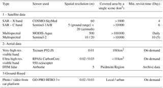
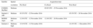
Table 2 Resume of satellite data in relation with the flood stage.

3.1 Flood mapping at a regional scale with satellite data

The developed methodology is based on a multiscale approach that starts from the use of low-resolution regional scale satellite images. The use of different available satellites images can support the identification of flood effects at a low-resolution over large areas and at higher resolution at a local scale. The choice of the most appropriate satellite data depends on different factors: (i) the characteristics of the study area, (ii) the spatial resolution, (iii) the revisit time, (iv) the time of the acquisitions with respect to the moment of maximum inundation and (v) the availability and cost of images.

In this paper, only free of charge images were used to assure a low-cost approach. For every considered dataset, we produced a map of the flooded area that represents the synthesis of remote sensing data and geomorphological evidence from the 5 m DTM available from the Piedmont Region. We use a visual-operator approach to map the flooded areas that resulted in more precision than automatic classifications, especially in the case of post-flood images. Table 2 presents the satellite data related to the flood phase. We considered as co-flood data all of the images acquired between early 25 November 2016 (start of the first inundation) and the evening of 26 November 2016 (the withdrawal of water).

3.1.1 SAR data

SAR instruments work in all-weather conditions and in the nighttime, thus ensuring a high observation frequency and increasing the opportunity of providing data corresponding with the flood event.

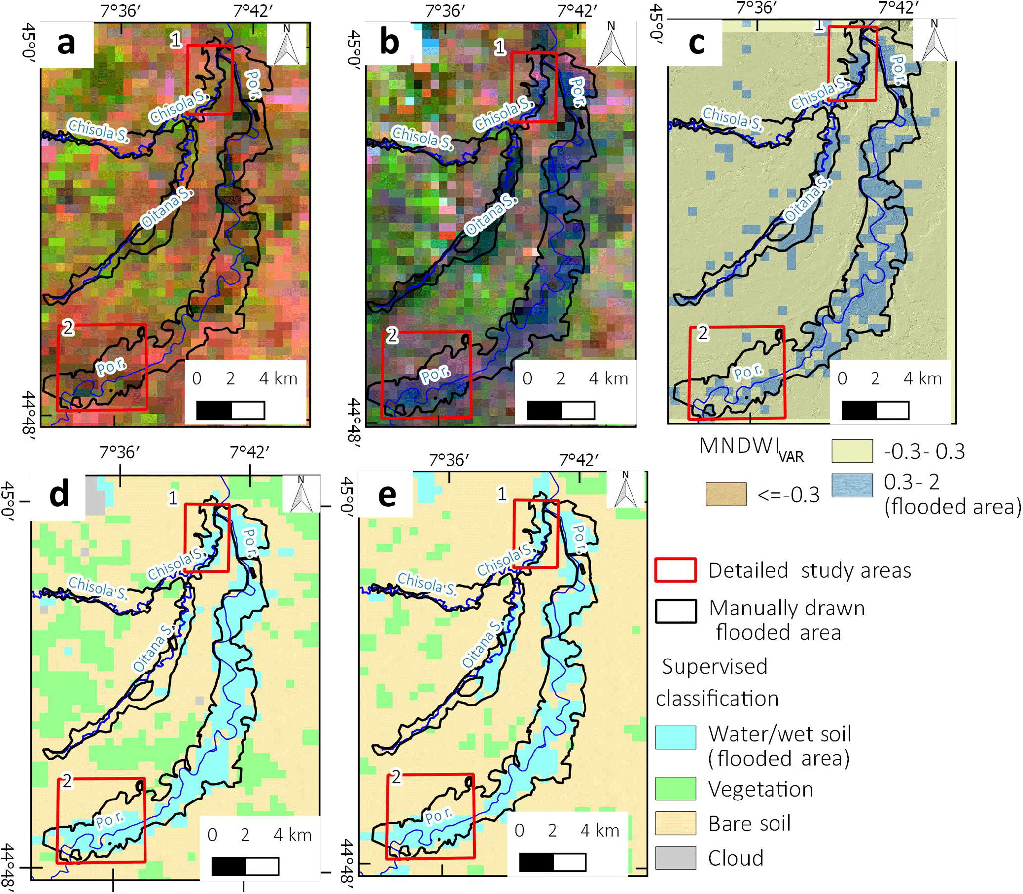
Figure 4 MODIS Aqua satellite image (a) false colour band composition 7-2-1 acquired on 12 November 2016; (b) false colour band composition 7-2-1 acquired during the 26 November 2016 event; (c) automatic detection of the flooded area using MNDWI_var > 0.3; automatic detection of the flooded area using supervised classification with maximum likelihood method (d) and with spectral angle method (e). The red box identifies the local case history of Moncaleri (1) and Pancalieri (2).

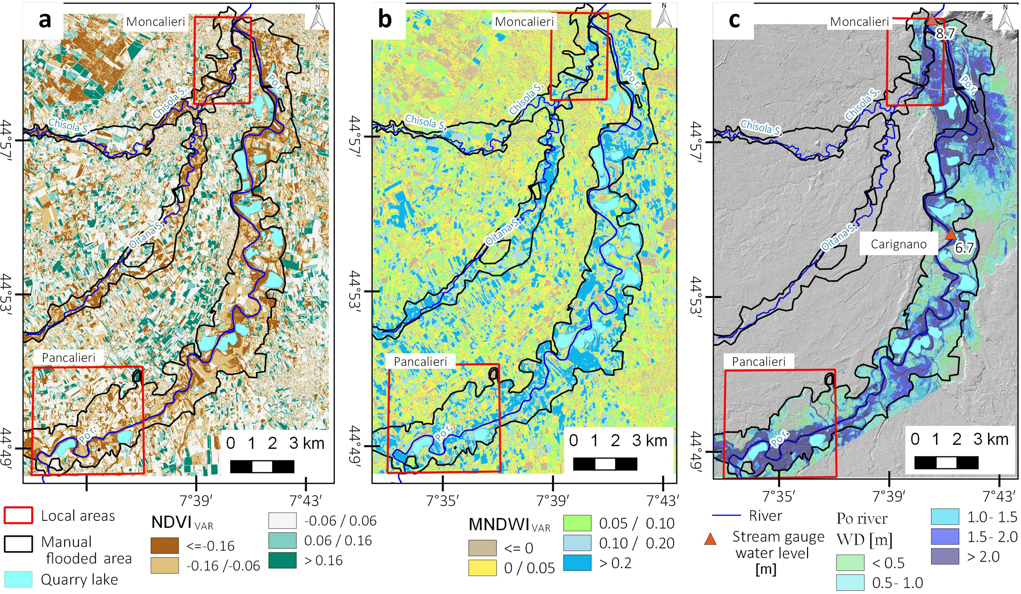
Figure 5 Sentinel-2 analysis and validation, (a) NDVI variation 10 m of spatial resolution, (b) MNDWI variation 20 m of spatial resolution, (c) Simulation of flooded area water depth for the Po River based on 5 m DTM and river height level registered in the Arpa Piedmont stream gauge.

(I) Co-Flood mapping. If data are available during the maximum flooding phase, it is possible to accurately map the affected area using high-resolution SAR images, such as those acquired by the TerraSAR-X (Giustarini et al., 2013) and COSMO-SkyMed (CSKM) (Refice et al., 2014) satellites. In particular, the identification of the flooded area is performed by analysing the SAR backscattering, which shows low values in water-covered areas. In our analysis, we used a SAR image acquired by the X-band COSMO-SkyMed satellites constellation (wavelength ∼ 3 cm) on 25 November 2016 (05:05 UTC acquisition time). Data were provided free of charge by the E-Geos and the Italian Space Agency (ASI) in a quick-look preview format with a 60 m × 60 m resolution.

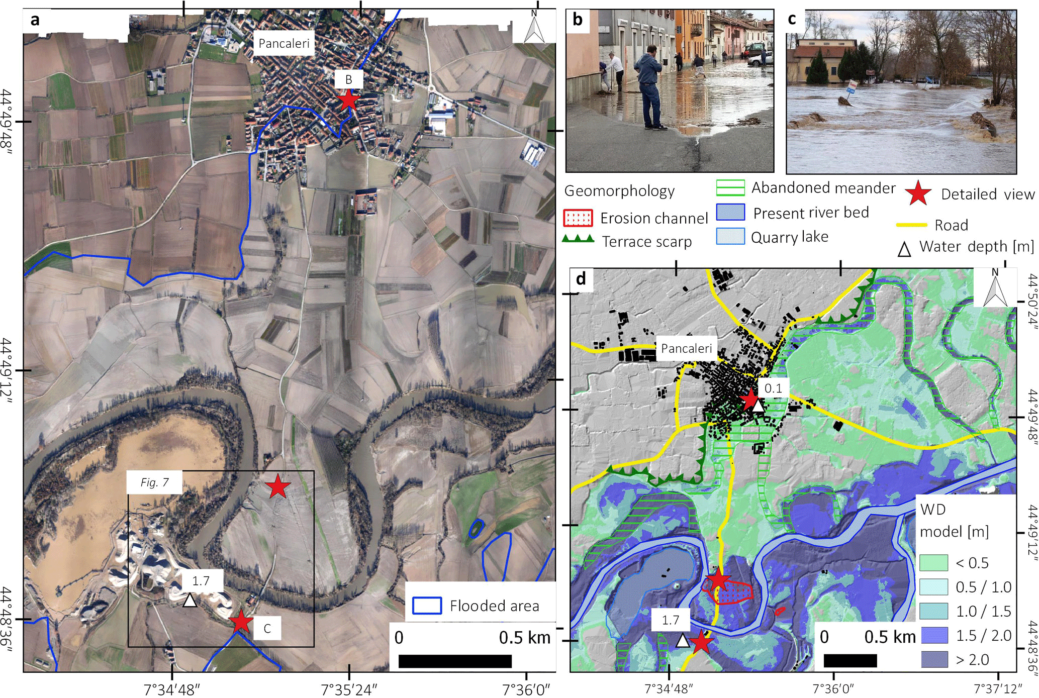
Figure 6 (a) Aerial photo at 10 cm of resolution taken 28 November 2016. Panels (b) and (c) are photos taken from a local newspaper and geo-localised with Google Streetview; (d) Geomorphological elements and model of estimated water depth (m).

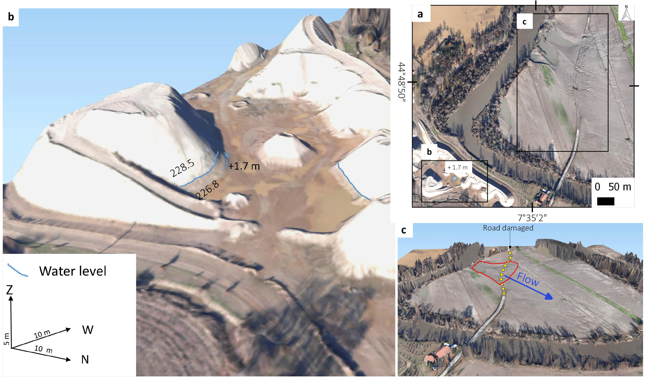
Figure 7 The SfM 3-D model obtained from the very high-resolution aerial photo, near the Po River at the south of Pancalieri. (a) Location of 3-D models; (b) the approximate measurement of water depth on sand deposits of a quarry (a); (c) the effect of meander cut: an erosion channel and the destruction along a stretch of road.

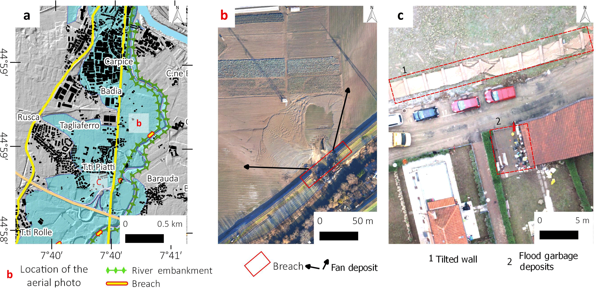
Figure 8 (a) Map of areas flooded by Chisola stream in Moncalieri municipality with location of detailed photo; (b) aerial photo at 0.1 m of resolution showing the breach of river embankment and the “alluvial fan” created by water flow showed with a 3-D view in Fig. 9; (c) RPASs photo at 0.02 m of spatial resolution showing a collapsed wall in the Tetti Piatti area and a deposit of damaged goods from the nearby house.

The CSKM data provided is a simple non-geocoded image in greyscale format (0–255). After the geocoding, we re-classified the SAR amplitude images through GIS software, using empirical thresholds in three main classes: water covered areas (0–60), soil and vegetation (60–160) and urban area (160–255). The investigated area is almost flat, thus it is not affected by problems related to geometrical distortions of backscattering. We validated the classification accuracy by comparing the reclassified images with an aerial photo, optical images, and land-use database. The analysis with such data notes the relevance of co-flood images for the fast mapping of flooded areas. It is not possible to know a priori if a co-flood image will be available during the maximum of the flood event. However, the short revisit times achieved by the new generation of SAR satellites can significantly increase the possibility of collecting co-flood data.

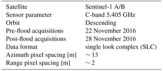
(II) Post-flood mapping. We also performed a post-flood mapping by exploiting data acquired by the Sentinel-1 Mission, which is composed of a constellation of two satellites, Sentinel-1A and Sentinel-1B, launched on 3 April 2014, and 25 April 2016, respectively. Sentinel-1 satellites have been designed to acquire C-band SAR data in continuity with the first-generation ERS-1/ERS-2 and ENVISAT Mission, developed within the European environmental monitoring program of Copernicus. The Sentinel-1A SAR operates at 5.405 GHz and supports four imaging modes providing images with different resolutions and coverages (Torres et al., 2012). We used the Interferometric Wide Swath Mode (IW) acquisition mode by employing the Terrain Observation by Progressive Scans (TOPS). The IW TOPS mode is the primary mode of operations for the systematic monitoring of surface deformation and land changes (De Zan and Monti-Guarnieri, 2006). This acquisition mode provides large swath widths of 250 km with a spatial resolution of 5 m × 20 m (IW). The repeat cycle of the twin Sentinel-1A/B constellation was reduced to 6 days.

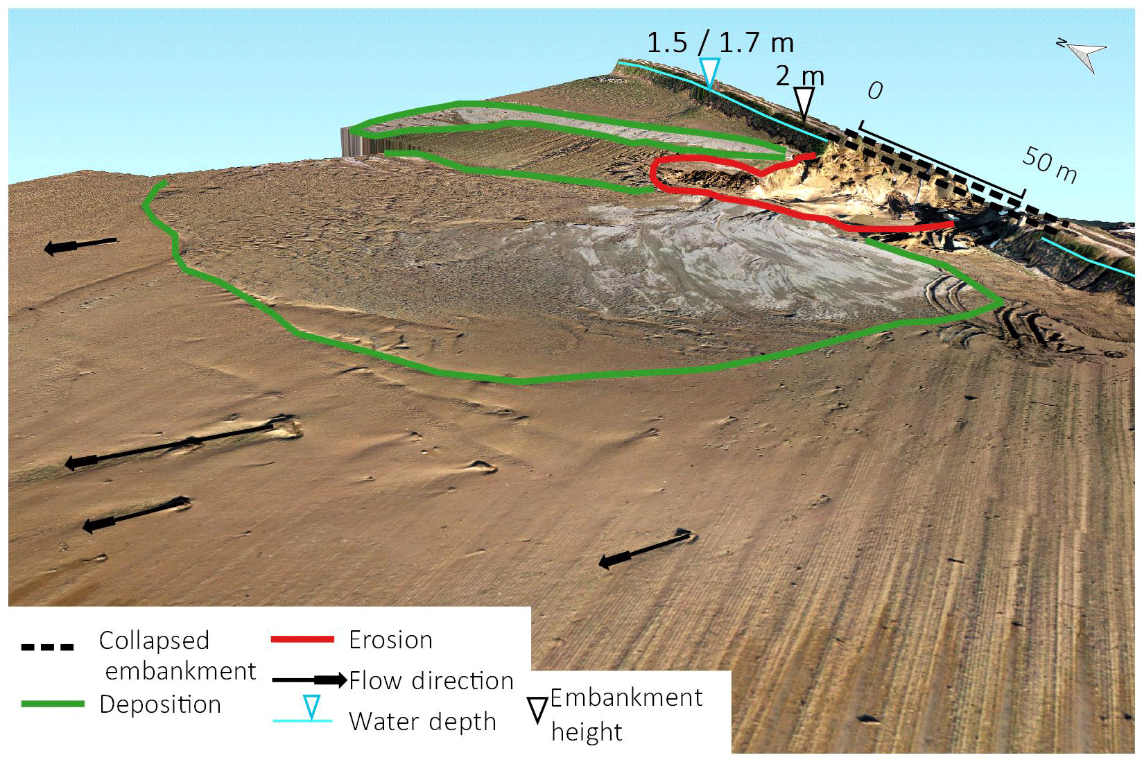
Figure 9 3-D Model derived from the RPASs aerial photo and SfM elaborations photo overlap. The model shows the river embankment rupture, point B in Fig. 8a, and the geomorphological effects in the neighbour areas. It is also possible to estimate the water depth from the signs on the embankment.

For our analysis, we acquired two IW Sentinel-1A/B images collected over the study area in VH polarisation along the descending satellite passes. In particular, we exploited the data acquired after (on 28 November 2016) and before (22 November 2016) the flooding event (see Table 3).

The SAR data, provided in the single look complex (SLC) format, were first radiometrically calibrated to convert the digital number (DN) values into corresponding backscattering coefficients, i.e. sigma naught (σ^o) values, which contain information on the electromagnetic characteristics of the surface under investigation. Subsequently, the calibrated SAR data were multi-looked with one look in the azimuth direction and four looks in range one, and finally geocoded, by converting the maps from radar geometry into universal transverse mercator (UTM) coordinates (zone 32T).

Table 3 Characteristics of the Sentinel-1 dataset used in this study.

After these pre-processing steps, to detect land surface changes induced by flooding, we computed the difference between the post- and the pre-flooding geocoded backscattering coefficient images, and produced the map of the temporal variation of the surface backscattering ($\mathrm{\Delta }{\mathit{\sigma }}_{\mathrm{post}-\mathrm{pre}-\mathrm{flooding}}^o$).

3.1.2 Multispectral satellite data

In this category, we considered both low- and medium-resolution images. Unfortunately, we found co-flood images only for the low-resolution images.

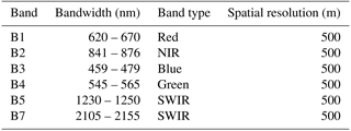
(I) Medium-low resolution satellite data. MODIS (Moderate Resolution Imaging Spectroradiometer) is a system of two sun-synchronous, near-polar orbiting satellites, called Aqua and Terra, that acquire images all over the world daily (Justice et al., 1998). Terra acquires images in the late morning, while Aqua acquires them in the early afternoon. The satellites also have a nighttime pass when they acquire images in the thermal bands. This repeat frequency does not occur along the same ground track, and the repeat cycle along the track is every 16 days. The high revisit time allows detecting floods with more probability over vast areas when they are still flooded and not covered by clouds. We searched for the first free-cloud MODIS images from the Earthdata portal of NASA (https://worldview.earthdata.nasa.gov, last access: 23 May 2018). The selected image was acquired by the Aqua satellite on 26 November 2016. We used the 6-bands products with a spatial resolution from 250 to 500 m that ranges from the visible to near-infrared (NIR) and shortwave infrared (SWIR) (Table 4). For the elaboration, we used the MYD09 – MODIS/Aqua atmospherically corrected surface reflectance 5-Min L2 Swath 500 m, (Vermote, 2015), downloaded from http://ladsweb.nascom.nasa.gov/ (23 May 2018). To have a benchmark of the non-flooded situation, we also used the Aqua satellite image of 12 November 2016, which was compared with the image taken during the flood. We did not apply an atmospheric correction to the images because the MYD09 product is adequate for our purposes. Moreover, the study area is small (20 km), and the atmospheric parameters for correction available at 1 km of spatial resolution (water vapour, ozone or aerosol) did not show a significant change. For the identification of the flooded areas, we made the following elaborations:

• a.

  a false colour image was made with combinations of 7-2-1 bands for a visual interpretation of flooded areas.

• b.

  modified normalised difference water index variation MNDWI_var (Eq. 1). The MNDWI allows the detection of water masses or soil moisture. In the literature, different combinations for this index have been presented and discussed (Xu, 2006; Zhang et al., 2016; Gao, 1996). In our study, we used the ratio between B1 (red band) and B7 (Short Wavelength Infrared: SWIR). The difference with a non-flooded situation can be used for identifying changes in the soil moisture. We used the results of the supervised classification to mask the cloud cover.

  $$\begin{array}{ll}{\displaystyle }& {\displaystyle }\mathrm{MNDWIvar}=\mathrm{MNDWIpost}-\mathrm{MNDWIpre}\\ \text{(1)}& {\displaystyle }& {\displaystyle }\mathrm{where}\mathrm{MNDWI}={\displaystyle \frac{\left(\mathrm{B}\mathrm{1}-\mathrm{B}\mathrm{7}\right)}{\left(\mathrm{B}\mathrm{1}+\mathrm{B}\mathrm{7}\right)}}\end{array}$$
• c.

  The supervised classification has already been used in the literature to map flooded areas using machine learning, as described in Ireland et al. (2015). In our work, we made a simple supervised classification with SAGA GIS. We first manually defined the training areas with the main land use typologies visible on the false colour image. We tried different methodologies for the classifications, and we chose as most accurate the maximum likelihood with the absolute probability reference and spectral angle methods. We validated the reliability of these classifications with a comparison with the false colour image and land-use database. Then, using a GIS query, we extracted the category “area covered by water or wetland” that mostly corresponded to the flooded area for accuracy statistics reported in Sect. 4 Results.

Table 4 Characteristics of the Aqua MODIS data used in this work.

(II) Medium-high resolution satellite data. Medium-high resolution multispectral satellites (e.g. Sentinel-2 A and B or Landsat 8) have a longer revisit time (from 5 days for the Sentinel-2 constellation to 16 days for Landsat-8). It is more difficult to have images at the same time of the maximum flood and that are cloud free. However, by comparing two images acquired before and after a flood event, it is possible to calculate the variation of different indices related to changes in the reflectance of the soil and/or of the vegetation. Thus, it is sometimes possible to map the flooded area indirectly (post-flood mapping).

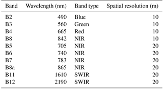
In our study area, we used images taken by Sentinel-2 before the flood (11 November 2016) and after (1 December 2016). Sentinel-2 has some bands at 10 m of spatial resolution and some bands and 20 m of spatial resolution (reported in Table 5). To detect the flooded area, we first made a visual interpretation using images with different bands' compositions of post-flood data. The comparison of the considered images allowed us to calculate the difference between the following two indices:

1. the normalised difference vegetation index (NDVI) variation. The NDVI was calculated with 10 m of spatial resolution images from Sentinel-2 using the near-infrared band (NIR – B8), and the red band (B4). The NDVI is related to the activity of vegetation. It is possible, by calculating its variation (Eq. 2), to identify the decrease of the NDVI values as an effect of inundation on vegetation (Ahamed et al., 2017). The detection of this change allows the mapping flooded areas indirectly.

   $$\begin{array}{ll}{\displaystyle }& {\displaystyle }\mathrm{NDVIvar}=\mathrm{NDVIpost}-\mathrm{NDVIpre}\\ \text{(2)}& {\displaystyle }& {\displaystyle }\mathrm{where}\mathrm{NDVI}={\displaystyle \frac{\left(\mathrm{B}\mathrm{8}-\mathrm{B}\mathrm{4}\right)}{\left(\mathrm{B}\mathrm{8}+\mathrm{B}\mathrm{4}\right)}}\end{array}$$

2. the modification of normalised difference water index (MDWI) variation. We used a similar index already tested for the MODIS data. We used Sentinel-2 to calculate the MNDWI considering the red edge band (B5) and the SWIR band (B11) at 20 m of spatial resolution. With this approach (Eq. 3), it is possible to map the variation of soil moisture related to recently flooded areas or areas that are still covered by water.

   $$\begin{array}{ll}{\displaystyle }& {\displaystyle }\mathrm{MNDWIvar}=\mathrm{MNDWIpost}-\mathrm{MNDWIpre}\\ \text{(3)}& {\displaystyle }& {\displaystyle }\mathrm{where}\mathrm{MNDWI}={\displaystyle \frac{\left(\mathrm{B}\mathrm{5}-\mathrm{B}\mathrm{11}\right)}{\left(\mathrm{B}\mathrm{5}+\mathrm{B}\mathrm{11}\right)}}\end{array}$$

Table 5 Characteristics of Sentinel-2 data used in this work.

3.2 Flood mapping at local scale with high- and ultra-high-resolution data

The flood mapping at the local scale was made using high- and ultra-high-resolution images.

Immediately after the event, a research project proposed by CNR-IRPI was conducted with the participation of ALTEC S.p.A., Digisky s.r.l. and the Civil Protection Agency of the Metropolitan City of Turin. The aim of the project is a methodological analysis of a possible low-cost solution that could be used for the high-resolution mapping of flood effects.

The study started from the SMAT F2 Project results (Farfaglia et al., 2015), where different solutions for the acquisition of RGB datasets with small and medium remotely piloted aerial systems (RPAS) were developed. Additionally, the previous experiences of the CNR IRPI and Civil Protection Agency in the use of small RPAS for the study of geo-hydrological processes (Giordan et al., 2015; Boccardo et al., 2015; Fiorucci et al., 2018; Giordan et al., 2017) were useful for the definition of a correct use of these systems. These previous experiences noted how the use of low-cost systems for the acquisition of RGB images and the application of SfM algorithm can be considered as a good solution for the creation of high-resolution 3-D models.

3.2.1 Aerial high-resolution images

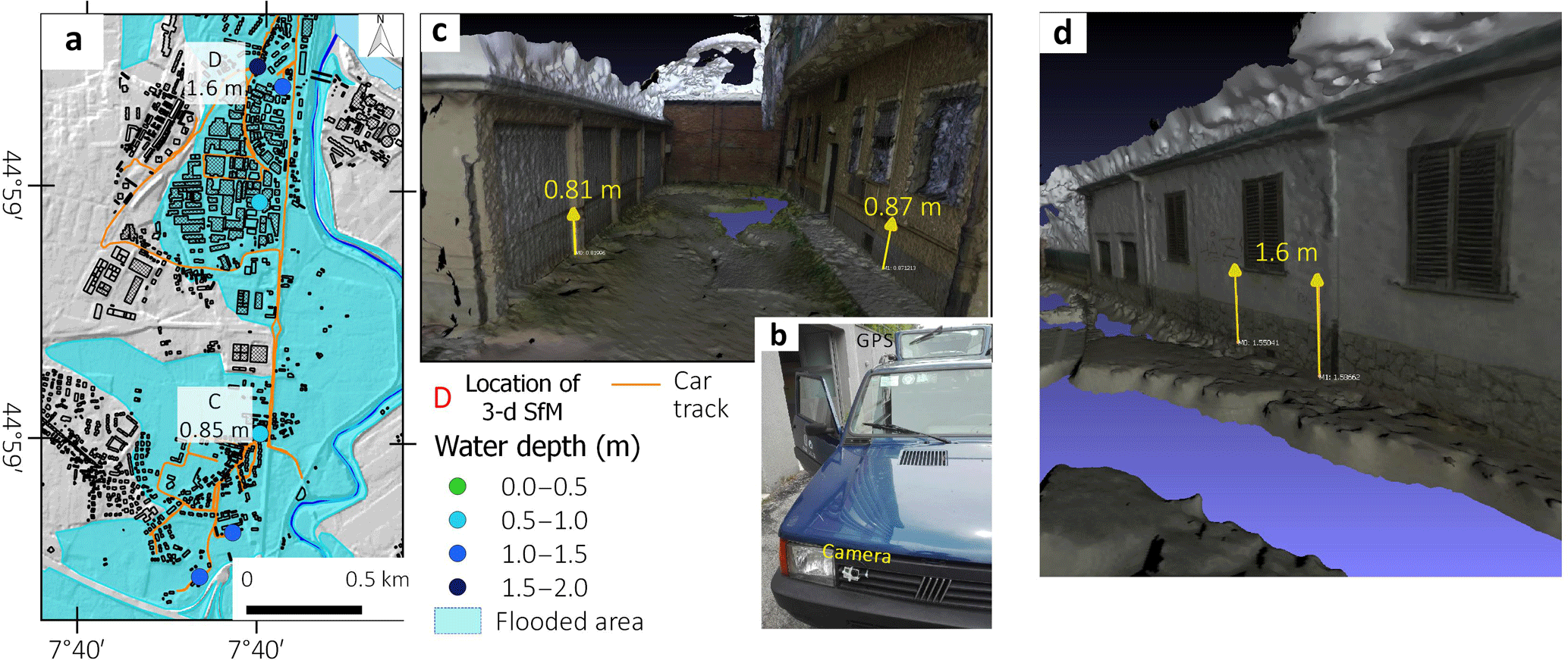
Figure 10 (a) Map of the flooded area by Chisola Stream in the Moncalieri municipality with measured water height and location of 3-D photo, (b) installation of the GO-PRO HERO 3+ (Black Edition) camera and GPS antenna over the car (the processing system for STANAG 4609 encoding was installed inside the car) (c) and (d) examples of 3-D models made with SfM in which it was possible to measure the water height.

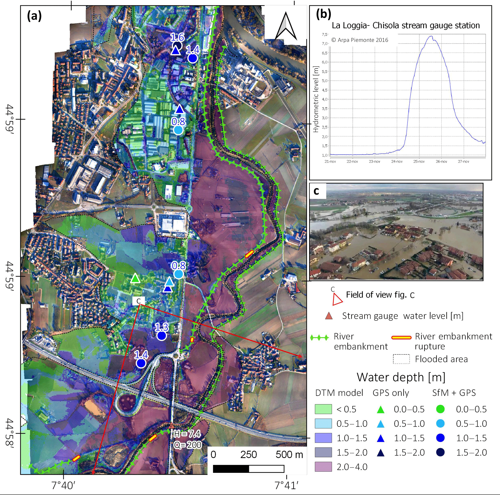
Figure 11 (a) Water depth levee map based on SfM data and 5 m DTM model. (b) Water level reached by Chisola Stream in ARPA Piedmont station. (c) Geolocated third part photo: 25 November 2016 aerial view of flooded area found on the web (https://vivere-moncalieri.it/2016/11/30/3760/, last access: 23 May 2018).

Aerial photos taken in a few hours or within a few days after the peak of inundation allow the mapping of flooded areas with high precision over the most involved territories. In our case, aerial photos were acquired after the flood over the Po River near the village of Pancalieri and for the town of Moncalieri. We used a low-cost aerial platform (Tecnam P92-JS) provided by DigiSky s.r.l., equipped with a 16 Mp mirrorless camera (Panasonic Lumix GX7) that allowed us to acquire aerial photos with a spatial resolution of 10 cm pixel⁻¹. The system also has an onboard GPS that acquires image shooting points and allows the georeferencing of the photos sequence using SfM.

The use of a manned solution has several added advantages that can be very useful in this phase: (i) it is possible to fly over urban areas without the strong limitations that characterise RPAS; (ii) the system can acquire images over large areas within a limited period of time; and (iii) the system can fly on demand during the flood or immediately after (with favourable weather conditions).

The adopted solution was used to acquire images of the 9.2 km² of the most damaged area of Moncalieri and 9.5 km² of the flooded area of Pancalieri. These two areas are representative of different conditions:

1. the area of Pancalieri is a rural area mainly dedicated to agriculture. In this case, the Po River flood covered large uninhabited sectors of the Pancalieri plain and reached part of the town of Pancalieri. Here, using SfM, the plane images were also processed for the creation of a digital surface model (DSM) (resolution of 20 cm) with the aim of mapping geomorphological features related to the flood.

2. the selected area of Moncalieri is a strong urbanised sector of the municipality. In this area there is (i) a motorway, (ii) several regional and local streets, (iii) a residential area with recent unfamiliar houses and small condominiums and (iv) an industrial and commercial district. The inundation of this area is due to the Chisola Stream levee's break. The map of Moncalieri was useful for the identification of the most damaged elements, and in particular the levee. In the most critical areas, we also used RPAS to acquire ultra-high-resolution images.

3.2.2 RPAS ultra-high-resolution images

In the ultra-high resolution step, we used the RPAS and the terrestrial system. The RPAS was used to acquire nadiral photo sequences of the most damaged areas and infrastructures. In particular, we tested the possibility of using RPAS for the identification of damage that occurred to the Chisola Stream levee and one of the most damaged sectors of the town of Moncalieri. The employed RPAS is a multi-rotor (CarbonCore 950 octocopter) equipped with a Canon EOS M (Sensor CMOS APS-C, 18 Mp). The system is equipped with a flight terminator and a parachute and can also be used in inhabited areas. The Civil Protection Service of the Turin metropolitan area provided the RPAS. The obtained aerial photos have a spatial resolution of 3 cm pixel⁻¹. Using SfM, the images of the drone were also used to create the 10 cm resolution DSM. All of the flood mapping methodology described above are very often unable to provide a consistent measurement of water depth. This limitation is not due to the resolution or the time of acquisition, but it is intrinsic in nadiral images. For this reason, in the Moncalieri area, we choose to deploy a ground-based solution.

3.2.3 Ground-based ultra-high-resolution images

As previously mentioned, we tested a low-cost terrestrial system for the acquisition of ultra-high-resolution images. In particular, we used an integrated system developed by ALTEC SpA, which couples a Go-Pro HERO 3+ (Black Edition) camera with a GPS and an acquisition module. The system is able to record a STANAG 4609 geolocated HD video. We installed the experimental system over a CNR IRPI car, and a survey was performed a few days after the flood in the study area of Moncalieri. The continuous record of geolocated videos can be a good solution for the acquisition of a significant amount of data immediately after the flood when marks of the water level are still clearly visible along building facades. The identification of water levels of flooded areas based on the measurement of marks over facades is not a novelty, but the manual acquisition of these data has often been a critical task. Citizens often want to quickly obliterate these signs as a reaction to the life-threatening experience that they lived through. The use of field teams that look for these marks can be a time-consuming task that can produce few results with considerable effort because before the survey it is hard to have an idea of the number and the distribution of facade marks that can be identified and measured. The number of marks strongly decreases after a few weeks, and for this reason, it is essential to have a system that can acquire very fast geolocated images and that can be easily used over large areas.

The presented system is straightforward and efficient. Other components of the team can analyse the geolocated video immediately after the acquisition or many days afterwards. The primary goal is the fast acquisition of numerical information of the flood effects that can be used for several purposes. For the identification and mapping of water levels, the video is analysed, and a frame sequence is extracted from it when the operator sees some marks left by water over the facades. The developed system can extract not only frames but also their geocoding information, which are computed using SfM applications. The result is a georeferenced 3-D model of the facade that can be used to measure the water level with a good approximation (few cm). We validated the accuracy of measurements of the water level based on SfM with manual measurements accurately geolocated with GPS RTK positioning.

3.2.4 Field data

Field survey and ancillary data, such as measurements of river discharge stations and civil protection reports, were used to validate the maps derived from remote sensing interpretation and the simulation models for the Pancalieri and Moncalieri areas. We made a GPS RTK campaign in the Tetti Piatti and Tagliaferro areas to have direct measurements of the flood marks. In particular, we acquired the 3-D position of marks previously identified using the available video. We used third party materials, such as newspaper reports, photos and videos found on the web with a validation of their reliability regarding geolocation and time. Available data were used to check the extension of flooded area and water height mapped with other methodologies.

3.3 Water depth models based on DTM approach

As previously mentioned, the primary goal of the presented methodology is the definition of the maximum depth reached by the water during the flood. The map of water maximum depth (WD) is an important document that can be used for the first definition of damage and remedial actions. All the acquired material, and, in particular, data that define the water depth reached by the flood, were used to calculate the water maximum depth map. In our study, we adopted a simple raster-based model (Bates and De Roo, 2000), and we created an absolute water level (WL) raster. The first step is the acquisition of several measurement points of water level (WL_p) that are calculated from the measured water depth point (WD_p). WD measurements can be performed using the following methods: (i) georeferenced photos (low accuracy); (ii) ultra-high-resolution measurements derived from SfM and integrated with a manual measured geolocated GPS RTK positioning (high accuracy); (iii) civil protections reports (the level of accuracy can be very different) and (iv) data acquired by hydrometric river level monitoring stations. Starting from the collected spotted measurements and the 5 m lidar DTM freely provided by the Piedmont Region, we calculated the WL value for each point using a simple formula: WL_p= DTM + WD_p. The available WL points were used to create the water level contour lines and then interpolated using GIS software to obtain the raster of the WL gradient. The WL raster is used to create the raster map of water depth, which can be calculated with a simple raster calculator of GIS software using the reversed formula WD = WL − DTM. The WD map is necessary information to assesses and improve the limit of the flooded area, and it is also fundamental for the phase of the preliminary damage assessment. We produced maps of the water depth at a medium resolution for the Po River (Fig. 5) and high resolution for the Moncalieri (Fig. 11) and Pancalieri areas (Fig. 6).

4 Results

4.1 Flood mapping from low to medium-high resolutions with satellite data

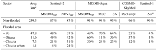
The satellite data allowed mapping of the flooded areas by the Po River, and the Chisola and Oitana streams, with a resolution that ranges from 500 m of MODIS to 10 m of Sentinel-2. We compared raster maps based on the remote sensing data with our perimeter of the flooded area (black polygon in Figs. 3, 4 and 5). We manually extrapolated the flooded area perimeters considering both satellite data and geomorphological features observed in the hillshade model derived from 5 m DTM of the Piedmont Region. For the evaluation of automatic flooded area maps based on satellite data, we applied a GIS query for each map to create boolean rasters of the flooded and non-flooded areas. Then, we overlapped the obtained raster with manual polygon for a geo-statistical analysis, as each polygon is reported with the percentage pixel classified as flooded or non-flooded. The main results are reported in Table 6.

Table 6 Accuracy in automatic flooded and non-flooded area detection.

For the Po River and part of Chisola Stream, we also mapped the flooded areas with the help of the WD model based on DTM. At the writing of this paper (November 2017), an official delimitation of flooded areas is still unavailable; a map made by ARPA Piemonte is under validation, and the data will be downloadable in the next months.

4.1.1 Flood mapping with SAR data

(I) Co-flood mapping, the reclassified amplitude of CSKM data. The image classification allowed us to detect three classes of SAR amplitude (Fig. 3a) that were defined by means of empirical thresholds: (i) low, that correspond to water covered area (blue); (ii) intermediate, such as soil and vegetation (green) and (iii) high, that are urban areas (pink). In the map (Fig. 3a), we also overlapped the quarry lake from ancillary data (cyan). The accuracy in the correct detection of land-use type is quite good, ranging up from 80 % for soil and vegetation, and 67 % for the urban area to 61 % for the water body (tested in quarry lakes). Vegetation and buildings are factors that reduce the detection of water covered areas even using full-resolution images and more complex processing (Pierdicca et al., 2018). In a second step, we selected, with a GIS query, the low resolution (water covered) class that mostly corresponded to the inundated areas and we compared them with the real flooded area. Additionally, the accuracy detection of the flooded areas is quite good: it ranges from 57 % in the lower Oitana Stream to 2 % in the Po area near Moncalieri. The low accuracy for some areas is related to the time of the satellite acquisitions (05:05 UTC of 26 November 2016) at some hour before the flood peak. The flood wave positions can be appreciated, especially along the Po River, where upstream (near Pancalieri) approximately 42 % of the flooded area was detected, while downstream (Carignano) it decreased to 4 %. The urban area of Moncalieri limits the capability detection of inundated areas. The false positive errors are less than 5 % of the area.

(II) Post-flood mapping with Sentinel-1 data. The map of the post- and pre-flood SAR backscatter difference ($\mathrm{\Delta }{\mathit{\sigma }}_{\mathrm{post}-\mathrm{pre}-\mathrm{flooding}}^o$) through the application of an empiric threshold allowed us to detect areas covered by water, i.e. flooded (Δσ^o<−1 dB) (Fig. 3b). Such results show that most of the areas classified as flooded by the co-flood analysis were no longer covered by water on 28 November 2016. Only small depressed areas, e.g. ancient meanders of the Po River, were still flooded (Fig. 3b', 3b” and 3b”'). The case of Pancalieri will be discussed in more depth in Sect. 4.2.

4.1.2 Flood mapping with multispectral data

(I) Multispectral low resolution, MODIS-Aqua. The MODIS-Aqua satellite took an image reasonably free of clouds, over the entirety of the Piedmont region during the late morning of 26 November 2016. The image allowed the detection of the flooded areas with a resolution of 500 m.

From the false colour images (Fig. 4b), even if the area at the south of Turin was not yet directly flooded, it was only possible to detect that the soil was saturated with water (dark green–blue in false colour composition). The comparison with the pre-flood image of 12 November 2016 (Fig. 4a) improved the detection of the flooded area.

We also tried to extract, in an automatic way, the flooded area with the equations previously described.

We identified the flooded area using a GIS query with the value MNDWI_var≥ 0.3 (Fig. 4c). This value is an empirical threshold that allows the selection of most of the flooded area and minimises false positive errors. The results show a good correspondence between the manually drawn and the automatically classified flooded area; however, approximately 35 % of the flooded area was not identified. The mismatch can be explained with the satellite acquisition at the end of the co-flood stage when water started to withdraw. It is also possible to see some false positive pixels (< 10 %) that correspond to the shadow of the clouds or haze that was not possible to entirely filter out.

We also made a supervised classification of the 26 November MODIS image using the maximum likelihood (MLC) (Fig. 4d) and spectral angle (SA) (Fig. 4e) methods. In the study area, we classified four primary land covers: vegetation, bare soil, clouds and water bodies or wet soil that almost identify the flooded sector (the water bodies such as the quarry lakes are too small for MODIS pixel). After a visual checking of the classification reliability, we used a GIS query to select the “water covered and wet areas” class. The query created a Boolean raster of flooded areas. The accuracy of the flood map based on supervised classification was good, it identified most of the flooded areas for the Po River (>70 %) with low false positive pixels (Table 6). We obtained worse results for the area flooded by the Chiosla and Oitana streams.

For both indices, it is possible to see that the town of Moncalieri (red square 1 in Fig. 4) that was flooded by Chisola Stream is not well identified.

(II) Multispectral medium-high resolution post-flood mapping Sentinel-2. We analysed the data of Sentinel-2 by means of visual interpretation of RGB composite image, using two different indices (NDVI and MNDVI) to identify the flooded areas (Fig. 5). For both indices, we used GIS queries with empirical thresholds to extract the flooded area:

1. NDVI variation (NDVI_VAR) at 10 m of spatial resolution (Fig. 5a). The results show that for the Po, Chisola and Oitana a clear pattern of negative NDVI variation corresponds to the flooded area. The study area is almost flat and mostly occupied by cultivated fields and in November it was characterised by a tillering of wheat. The flood caused the deposition of a thin layer of silt sediment that caused a decrease of vegetation activity (most of the flooded area shows an NDVI_VAR<−0.06) that could be detected using the available dataset. In contrast, the wheat field outside the flooded area shows an increasing or stationary NDVI. In the maps are the visible negative NDVI_VAR and also outside the flooded area are related to a (i) winter decrease of activity of natural vegetation or some cultivations and (ii) the longest building shadow in the urban areas. The presence of false positives hampers the use of automatic classifications of flooded areas, and a visual interpretation is necessary. It is possible that flood effects and the layers of silts could have also affected the crop productivity with relative economic damage, as reported in other cases (Tapia-Silva et al., 2011; Shrestha et al., 2017), but this evaluation is not the aim of this study.

2. MNDWI variation (MNDWI_VAR) at 20 m of spatial resolution. The index is directly related to the presence of water or high soil moisture. The results show that for the Po, Chisola and Oitana floodplain (Fig. 5b), there is a clear pattern of positive MNDWI_VAR that indicates an increase of soil moisture and the presence of some areas that were still inundated. It is possible to see that a threshold of MNDWI_VAR+ 0.1 is the best to delimit the flooded areas. However, as with NDVI, the presence of many areas with positive variations outside the flooded sector makes more accurate a manual interpretation compared to an automatic classification. The evidence also suggests that for this index, it is important to have images taken within few days after the flood when the affected areas are still covered by water or with very wet soil. Table 6 shows the accuracy statistic for the automatic mapping of flooded areas based on satellite data: MNDWI shows slightly better accuracy than NDVI. Note that for both MNDWI_VAR and NDVI_VARthe flooded area is well detectable in and around the village of Pancalieri (>50 % of accuracy) where land use is mostly cultivated land. In contrast, it is more difficult to detect the flooded area in the highly urbanised town of Moncalieri (<20 % of area detected).

(III) Water depth model. We created a WD model for the Po River (Fig. 5c) following the procedure described in Sect. 3.3. The simulated WD model has a good match with the benchmark polygon and the evidence from Sentinel-2 (Fig. 5a and b) and MODIS data (Fig. 4). It is also possible to observe some discrepancy at the southeast of Moncalieri, where a large area should be flooded according to the model, but in reality was not affected. This mismatch could be explained by the presence of artificial structures (e.g. embankments) that protected the flood-prone areas and that our model cannot simulate. The uncertainty of our WD model is complicated to evaluate because it depends on many factors: the main limit is the number of ground-based WD measurements, their reliability and their geolocation. The interpolation to obtain the water table is also another source of error. The accuracy of the lidar DTM in the Piedmont Region ranges from ±0.3 m to ±0.6 m elevation in urban areas. Over this vast area, we do not have a ground measure for validation, but it is possible to estimate it from some photos found on the web that shows the model error is approximately 0.5 m. In the high-resolution WD model of Pancalieri and Moncalieri, shown in Sect. 4.2, it was possible to validate data with ground-truth evidence.

The final limits of the flooded area are the result of both remote sensing and WD model interpretation. Its accuracy can be considered acceptable for large cultivated and flooded areas by the Po River but it is less accurate for urban zones, especially in Moncalieri, where a local high-resolution analysis is needed to quantify the severity of the flood.

4.2 Flood mapping at local scale with high-resolution data

Inside the area analysed using remote sensing systems, we chose the most critical sectors of Moncalieri and Pancaleri to test the high- and ultra-high-resolution images. As previously mentioned, the high resolution has been acquired using an aircraft, and the ultra-high resolution using RPASs and a ground-based photosystem. All of the images were processed using SfM that allowed us to obtain orthophotos and 3-D models.

4.2.1 High-resolution aerial photo, Pancalieri

The Po River partially flooded the village of Pancalieri on the morning of 25 November 2016. We mapped this area using high-resolution aerial photos (10 cm pixel⁻¹, RGB bands) provided by DigiSky. Aerial photos were taken 28 November 2016 (Fig. 6a) and allowed us to refine the map of the flooded area from the medium-resolution maps obtained with the interpretation of the Sentinel-2 data. With the help of DSM at 0.2 m of spatial resolution derived from SfM, we also mapped geomorphological features, such as erosion (meanders cut), deposition areas and road damage (Fig. 7c). The integration of the aerial photo and DSM also allowed us to make a 3-D model, in which it was possible to measure the water depth for some points where the water level marks are well detectable (Fig. 7b).

Using the procedure described in Sect. 3.3, we produced a WD model for the Pancalieri area (Fig. 6d) with higher accuracy with respect to the rest of the Po Valley. The higher accuracy of the model was obtained using: (i) high-resolution aerial photos; (ii) spot measurements derived from SfM; and (iii) different videos and photos found on the web and geo-localised with the help of Google Streetview (e.g. Fig. 6b and c). The model shows that there was a modest height of the water-flooded part of the Pancalieri village (<0.5 m), while near the Po River, the WD reached 2–3 m with a fast flow that caused an erosion channel. From the map of the flooded area (Fig. 6d), note that during the flood, ancient meanders at the east of Pancalieri were reactivated, and as a consequence, some areas were flooded that are quite far from the Po River's main course.

Some months after the flood (April 2017), satellite photos available on Google Earth (0.5 m spatial resolution) still show some traces of the floods, such as erosion, and areas covered by sand deposits. The flooded area is much more difficult to identify and confirms the importance of acquiring data as soon as possible after a flood event.

4.2.2 High-resolution aerial photo and ultra-high-resolution RPAS 3-D models, Moncalieri

Some parts of Moncalieri municipality (Tetti Piatti, Carpice and Tagliaferro localities) were flooded in the late morning of 25 November by the Chisola Stream that breached its embankment in different points (Fig. 8b). On the left side of the Chisola, the area with a very dense residential and industrial settlement suffered severe damage. Civil Protection evacuated hundreds of people. In the evening of 25 November, The Po River flooded another sector of the Moncalieri municipality.

A few days after the flood, the area flooded by the Chisola was analysed with different methodologies.

1. High-resolution aerial photos. As in Pancalieri, on 29 November a very-high-resolution (0.1 m pixel⁻¹) aerial photo using the aerial platform of DigiSKY was taken over an area of approximately 9.2 km². The aerial photo allowed us to refine the map of the flooded areas (Fig. 8a) and to detect the points where the river embankment collapsed (Fig. 8b).

2. Ultra-high-resolution RPASs photos. On 3 December 2016, the RPAS acquired photos (resolution of 0.02 ∕ 0.03 m pixel⁻¹) over some of the most critical areas (e.g. Tetti Piatti – Fig. 8c) for precise mapping of the flood effects. In this area, ultra-high resolution allowed us to detect some of the damage, such as the toppling of a wall in a recently built urban area, or the waste accumulation derived from damaged objects initially located in houses or industrial warehouses. The presence of these deposits is clear evidence of the damage that occurred, as well as a confirmation that nadiral images are not able to supply a sufficient dataset for the identification and evaluation of damage in urban areas.

The DSM based on RPAS photos also allowed us to create a detailed 3-D model of the river embankment rupture (Fig. 9). The presented 3-D model confirmed that the level of the Chisola during the flood was very critical, with a difference of fewer than 0.5 m from the top of the levee. The maximum water level considered under the security limits suggested by Po River authorities is 1 m for the top of the embankment. The RPAS model also allowed us to map the geomorphological effects of the rupture of the embankment. In particular, the ultra-high-resolution photos (Fig. 8a) and 3-D model (Fig. 9) allowed us to map a massive erosion of a field near the break and a pseudo alluvial fan created by the flow of water.

4.2.3 Measurement of water depth with SfM model from terrestrial camera, Moncalieri

In the same days of the RPAS aerial photo campaign, a field survey using an integrated system provided by ALTEC S.p.A. installed on a car (Fig. 10b) was made in the same urban areas of Moncalieri flooded by the Chisola (Fig. 10a). The survey had the aim of measuring the maximum water level reached and making a rapid evaluation of the damage. The survey lasted approximately 1 h for 12 km of the path along the road of the most critical area hit by the flood.

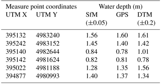
Where the level reached by the water was still visible over several facades (Fig. 10c and d), it was possible to estimate the maximum water level of the flood. During the first survey, we found 11 points where watermarks over facades were still visible. During the post-processing, we realised that the quality of the images extracted from the video was insufficient for the SfM application (the bit rate was too low and the frames are too pixelated). Therefore, after a month, we performed a second survey with a higher bit rate along the same path; however, only six marks were still visible (Fig. 10a). This reduction of available points confirmed that the delay between the flood and survey is a fundamental element that should be carefully considered because the number of possible pieces of information greatly decreases. For this second terrestrial camera acquisition, an improvement of the encoding quality was introduced. This improvement allowed us to extract high quality images compatible with the SfM application. We obtained 3-D models of the surveyed sectors, and we measured the high water marks on facades. Then, we validated the information obtained from SfM with a manual water height measurement geocoded with the GPS RtK systems for the six points and other additional five points. The accuracy of the measurement, considering that it is a low-cost solution and one of the first experimental uses of this system, is excellent; the average error comparing the SfM water level measurement with a manual measurement can be estimated to within a few centimetres (see Table 7).

Table 7 Water height measurements obtained from structure-from-motion, GPS survey and simulation with DTM.

4.2.4 High-resolution water depth models and ancillary data for damage evaluation, Moncalieri

The combined use of measurements derived from (i) a car camera elaborated with SfM, (ii) manual GPS RTK and (iii) the hydrometric level of Chisola Stream registered by ARPA Piemonte station (Fig. 11b) represents a useful dataset for the estimation of the WD. Using the 5 m DTM lidar of the Piedmont Region, we obtained the WL and the WD rasters (Fig. 11a). The result shows that in a large part of the analysed area, the water height was between 0.5 and 1 m. Unfortunately, in some morphological depressions, the level was higher than 1.5 m. The model also shows that in the cultivated area close to the left of the Chisola embankment, the water probably reached 2–3 m in height.

The water level map can suffer from some errors from spot measurements. These are related to the quality of DTM or the effect of local structures that can modify the water flow and height at a local scale. The comparison of the water level measured with SfM/GPS and the calculated level with DTM show variation within 0.2 m, a good result (Table 6).

Ancillary data, such as photos or videos found on the web (local newspaper, social media), and geolocated with Google Streetview, allowed us to improve and validate the map of the flooded areas and the height of the water (Fig. 11c). On the web, it is possible to find many photos or video of the flood event; however, only a small part of them can be geolocated with adequate precision and validated.

The water height map was crossed with a building database of the Piedmont Region to assign the average water height reached by the flood (Fig. 12a) on each building. The water height is one of the leading parameters that can be used for a preliminary estimation of the potential damage. We divided the water height into three main classes, corresponding to low (<0.5 m), medium (0.5–1.5 m) and high (>1.5 m), in terms of the damage expected. These thresholds have been empirically defined by Luino et al., (2009) and Amadio et al., (2016). The obtained map is a good representation of the level of damage caused by the flood that could be considered the final product of the presented methodology.

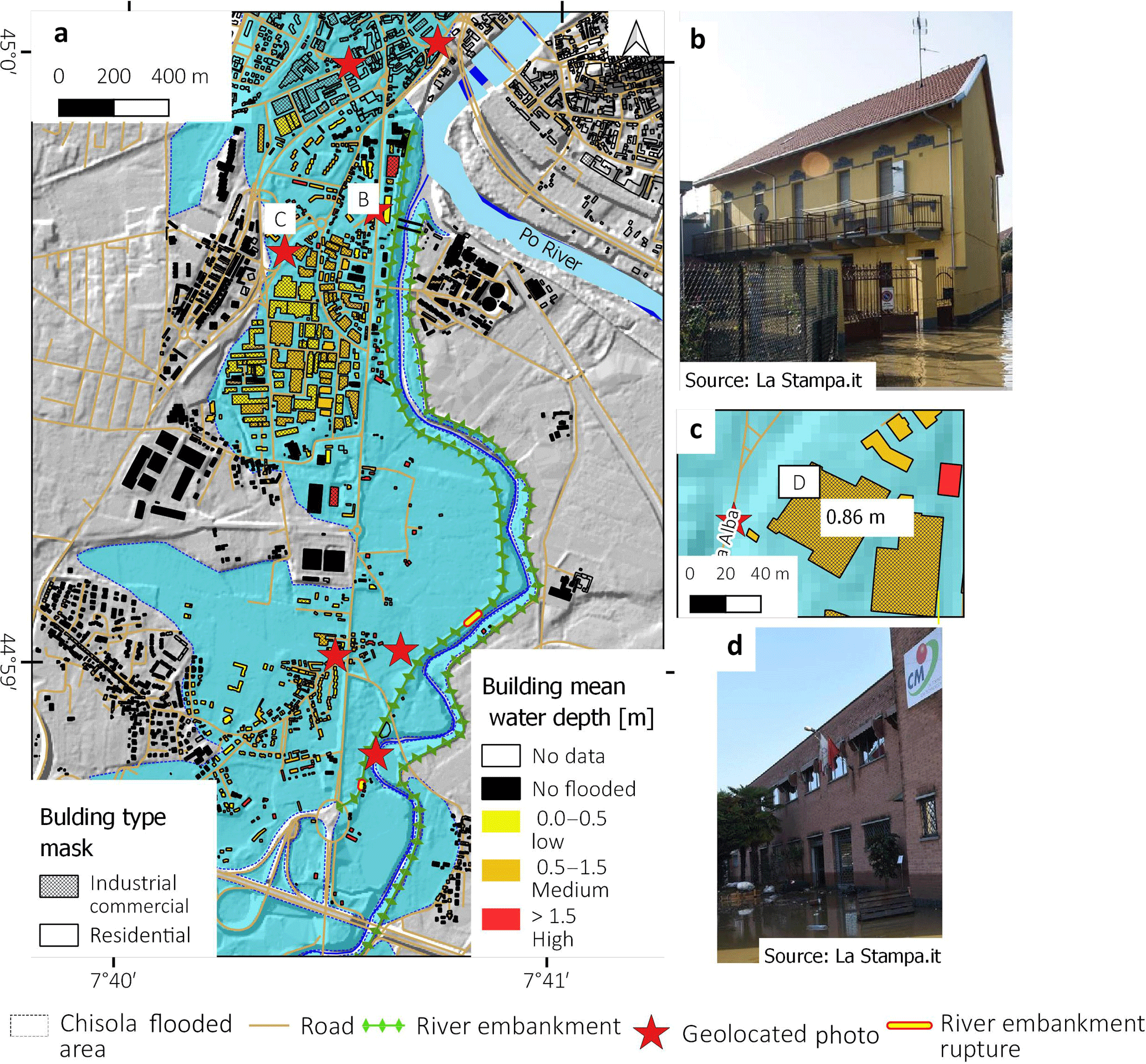
Figure 12 (a) Water level height map based on SfM data and 5 m DTM model; (c) Zoom on the building of panel (d); (b) and (d) Photo where it is possible to observe the water depth from the newspaper “La Stampa” geolocated using Google Streetview.

We compared this result with ground data where possible. For example, in the industrial warehouse shown in the focus map (Fig. 12b) it was estimated that there was an average value of 0.8 m water level (medium degree of damage expected). The evidence from a geolocated photo from the La Stampa newspaper confirms this value.

4.3 Flood mapping strategy flowchart

The flowchart (Fig. 13) shows the approach that we propose for the choice of instruments and methods to map the flooded areas, based on the results of this study. If free satellite data are available, it is possible to sort them, taking into account the parameters of time elapsed from the flood and the spatial resolution:

Figure 13 Flowchart of the proposed flood mapping strategy.

(I) The priority is to search for co-flood images that allow for easy mapping. In case of night and cloudy conditions, it is necessary to use SAR images (Sentinel-1), while for multispectral data acquired during the day, the choice is related to the spatial resolution. For example, Sentinel-2 or Landsat-8 data are more resolute than MODIS data.

(II) In the case of a post-flood satellite pass, only multispectral data can be used. Additionally, for post-flood data, the spatial resolution and time elapsed from the flood are the parameters that should drive the choice. The use of post-flood data implies more complicated post-processing (e.g. bands index variation) and the support of ancillary data and DTM to extract the flooded area map. In general, the rapid access to a data portal of free satellite data allows us to download the data and to make an evaluation of the best solution for the case under study; however, these data do not necessarily have a high spatial resolution.

After this step, it is possible to make the first delimitation of flooded areas, in the case that good data may include an already corrected and ready-to-use map. Then it is possible to focus the acquisition of on-demand of high-resolution sensors only in the most critical or unclear areas (case 2A of Fig. 13). If we use only on-demand data, without rapid satellite mapping, we could map large areas at a high spatial resolution (case 2B of Fig. 13). However, this solution implies a higher cost. In case of direct mapping at very-high resolution, it is better to use low-cost aerial platforms that are more flexible with respect to on-demand commercial satellites. The integration with DEM data allows the creation of the water depth model at the basin scale and a further refinement of flooded area maps (2C).

Urban area flood mapping (case 3 of Fig. 13) can be considered a hotspot priority inside the general flood map. It needs more accurate and high-resolution mapping with the use of ground-based measurements (such as the SfM model based on the car photos), RPAS survey and the creation of a water depth model that is essential for a precise flood magnitude assessment.

Note that it is not possible to select a priori which type of data and processing are better for flood mapping. The best method to use depends on different factors: (1) satellite acquisition and time elapsed from flood peak, (2) type of satellite data (SAR/multispectral, spatial resolution), (3) study area features and risk (dimension, cloud cover, land-use and element at risk) and (4) affordable cost (e.g. we used commercial satellite data or traditional aerial photos only if they give significant advantages to flood mapping).

5 Discussion and conclusions

In this work, we tested different methodologies for a low-cost and rapid flood mapping and water depth assessment using the November 2016 Piedmont flood as a case history. We used a multiscale and multi-sensor approach to find the pros and cons of each methodology in regard to the site conditions and available data. We also proposed a flowchart model to map flooded areas from satellites to ground-based data.

At the regional scale, satellite remote sensing showed a good performance in the flood mapping; the combined used of the SAR data of Sentinel-1 and CSKM, and multispectral data of MODIS-Aqua and Sentinel-2 allowed the creation of maps of the flooded area. The maps of flooded areas automatically extracted from remote sensing data were used with the help of DTM and a water depth model as a base map for an accurate manual drawing. In our study area (320 km²), approximately 66 km² were flooded by the Po River and the Chisola and Oitana streams. The WD models show that some areas were flooded up to 2 m of water height.

Concerning SAR data, we reclassified a simple preview low-resolution CSKM amplitude image acquired some hours before the co-flood time. The results show that the time of satellite pass is fundamental if the area is covered by water (such as the upstream part of Po River), up to 60 % of the pixels was correctly classified as flooded, and it was possible to observe a definite pattern. We compared pre- and post-flood SAR images of the Sentinel-1, making SAR the backscattering difference of radiometrically calibrated images. The result shows that SAR is weaker for post-event mapping; in our case 3 days after the flood (Sentinel-1), less than 4 % of the flooded area was still detectable. By considering the obtained results, it is also clearly important to have free and constant SAR satellite data provided by a national agency. A short revisit time and a constant acquisition are factors that increase the probability of having a SAR image for real-time flood mapping. For example, the two Sentinel-1 satellites provided free images every six days all over Europe, while other satellites have quite high costs and the acquisition is often on-demand. Moreover, most of the time, the on-demand acquisitions are activated only when authorities activate an emergency procedure (e.g. the EMSR of the European Union or by civil protection).

The low-resolution MODIS image acquired near the co-flood stage allowed a good identification of the flooded areas using different methods: MNDWI variation and supervised classifications. The detection accuracy is good, especially for the area flooded by the Po River where approximately 70 % of the flooded area was correctly identified.

Medium-high-resolution multispectral data have more capability with post-event images. In this work, we tested NDVI and MNDWI variations for the detection of flooded areas, based on the comparison of pre- and post-event images. Both methodologies show quite good performance in cultivated land (40–45 % of accuracy). Here, it was possible to detect a clear pattern: inside the inundated area, the percentage of pixel classified as flooded was 4 times greater than in the non-flooded area. The inundated areas are more difficult to detect in the dense urban area of Moncalieri (only 4 % of the area was correctly mapped). The water depth model of the Po River and DTM helped greatly in the improvement of the flood map based on remote sensing data. In the last few years, the revisit time for free multispectral data was sharply reduced (Landsat-8 has a revisit time of 16 days and Sentinel-2 has a revisit time of 5 days from March 2017 with the launch of the second satellite). This increases the probability of having an image free of clouds within few days or weeks after the flood or, in some cases, during the inundation phase. At the local scale, flood mapping showed a good agreement with regional scale mapping.

The high-resolution aerial photo and ultra-high resolution aerial photo from RPAS allowed the mapping of the flooded areas with more precision. The application of SfM allowed creating high-resolution DSM that was useful to map the geomorphological effects (e.g. meander cuts) and the widespread damage (embankment ruptures) in the Pancalieri and Moncalieri areas.

In the urban area of Moncalieri, where satellite data have a low accuracy, and precise evaluation of water depth is necessary for flood damage evaluation, the solution is the integration with ground-based data. In our work, we tested a low-cost solution with a GO-PRO HERO 3+ (Black Edition) camera installed on a car that allowed us to make 3-D models and to measure the water height reached during the flood. These measurements, validated with GPS, showed good accuracy, but it is necessary to do the survey within a few days after the flood when many water signs are visible. A proposal for the future is to use this system during the emergencies, for example on a civil protection car, to have a map of the water depth with a much higher density of points.

Using these measurements and a high-resolution DTM, it was possible to generate a raster model of water depth that has a good match with the ground truth, with approximately ±0.2 m of accuracy. We used the WD model results for a preliminary evaluation of building damage. The model could also be used in the future for flood prevention policies or civil protection plans.

Finally, from our work the importance of collecting ancillary data from the new sources on the web is also clear and the photos and videos collected during the flood by local citizens can be a great help in the validation of flooded area maps.