Predicting the thickness of shallow landslides in Switzerland using machine learning

Landslide thickness is a key variable in various types of landslide susceptibility models. In this study, we developed a model providing improved predictions of potential shallow-landslide thickness for Switzerland. We tested three machine learning (ML) models based on random forest (RF) models, generalised additive models (GAMs), and linear regression models (LMs). Next, we compared the results to three simple models that link soil thickness to slope gradient (Simple-S/linear interpolation and SFM/log-normal distribution) and elevation (Simple-Z/linear interpolation). The models were calibrated using data from two field inventories in Switzerland (HMDB with 709 records and KtBE with 515 records). We explored 39 different covariates, including metrics on terrain, geomorphology, vegetation, and lithology, at three different cell sizes. To train the ML models, 21 variables were chosen based on the variable importance derived from RF models and expert judgement. Our results show that the ML models consistently outperformed the simple models by reducing the mean absolute error by at least 20 %. The RF models produced a mean absolute error of 0.25 m for the HMDB and 0.20 m for the KtBE data. Models based on ML substantially improve the prediction of landslide thickness, offering refined input for enhancing the performance of slope stability simulations.

1 Introduction

Rainfall-induced spontaneous landslides pose serious threats to infrastructure and inhabited areas worldwide (Froude and Petley, 2018; Emberson et al., 2020). In Switzerland, landslides regularly cause extensive infrastructure damage and closures, evacuations, and even fatalities. For instance, 74 people died as a result of 40 different landslide events between 1946 and 2015 (Badoux et al., 2016). In August 2005, shallow landslides and the resulting hillslope debris flows caused damage amounting to USD 167 million across Switzerland within 48 h (Bezzola and Hegg, 2007). Approximately USD 17 million is spent each year on landslide protective measures in Switzerland (Dorren et al., 2009). To mitigate this risk, regional landslide hazard mapping and modelling provide an important basis for indicating potential hazard areas (Dahl et al., 2010; Kaur et al., 2019; Shano et al., 2020; Di Napoli et al., 2021). In Switzerland, national-scale shallow-landslide modelling was carried out within the SilvaProtect-CH project (Dorren and Schwarz, 2016). Results from this project have provided an important basis for, among other things, the delimitation of landslide protective forests across the country and preliminary risk analyses for national roads (Arnold and Dorren, 2015) and railways.

1.1 Background on landslide failure thickness

In general, landslides can be defined as the movement of a rock or soil mass along a slope (Varnes, 1978; Hungr et al., 2014). The term shallow landslides typically refers to translational sliding movements of soil material (earth and/or debris) from the upper soil layers, characterised by a well-defined sliding surface (Cruden and Varnes, 1996; Hungr et al., 2014). Often, shallow landslides result in hillslope debris flows, which can be very destructive because of their velocity and resulting impact pressure (Zimmermann et al., 2020). Landslides are usually classified as shallow landslides if the thickness of the instable mass does not exceed 2 m, which is also used as a definition in Switzerland (Lateltin et al., 2005). However, in some cases, the failure plane lies within the top 3 m (Sidle and Ochiai, 2013; Rickli et al., 2019; Li and Mo, 2019). With a median release area of around 200 m² and an average thickness of 0.5 to 1 m, shallow landslides generally fall into the category of small (10⁰–10³ m³) landslides, as proposed by McColl and Cook (2024). Occasionally, they can fall into the category of very small (10⁻³–10⁰ m³) or medium (10³–10⁶ m³) landslides. In this study, we define landslide thickness as the average thickness of the instable mass measured perpendicular to the original slope surface down to the failure plane (T_L in Fig. 1).

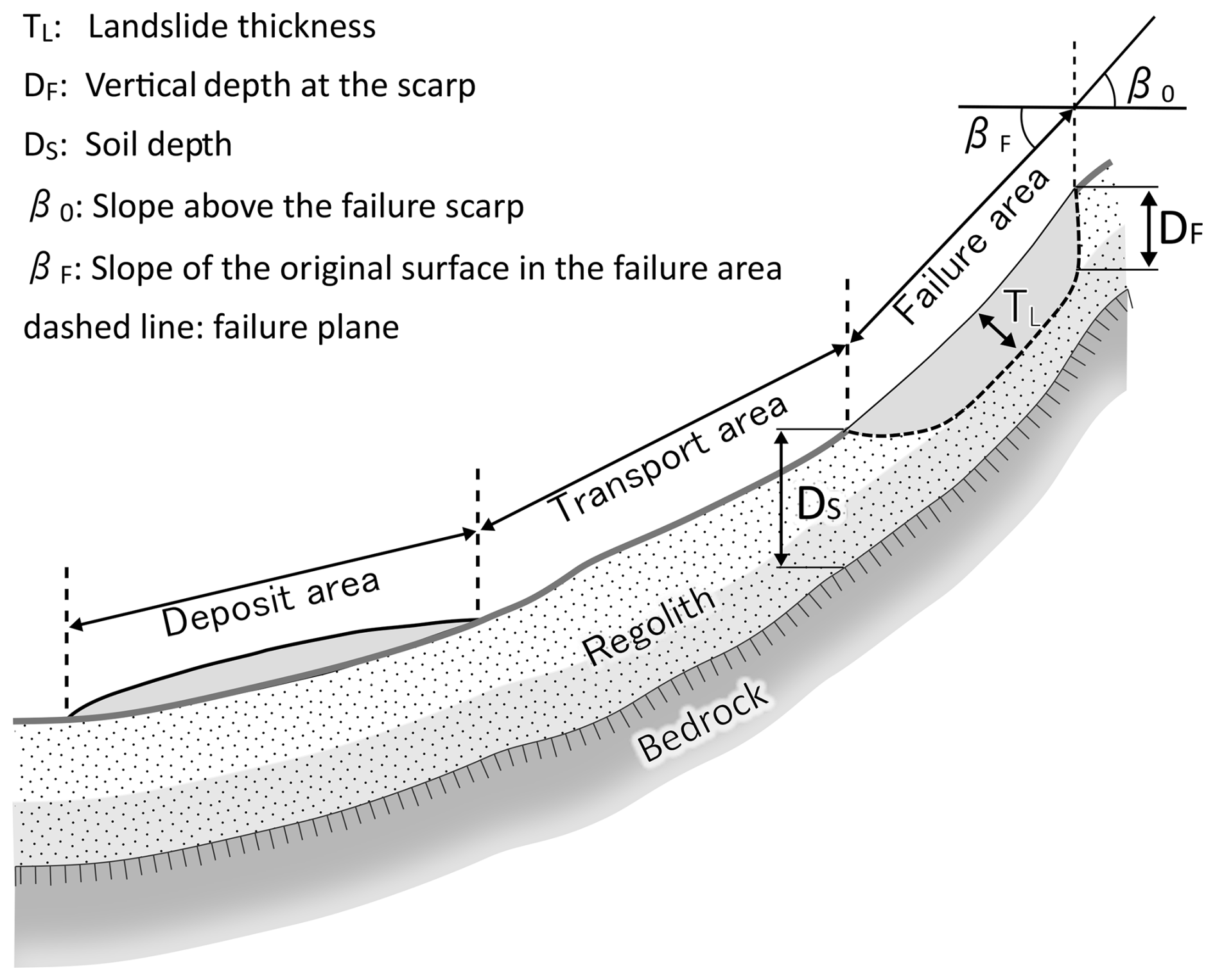
Figure 1 Schematic representation of a shallow landslide with its failure, transport, and deposit area, including important definitions used in this study. Variations in shading reflect differences in soil characteristics.

The basic disposition for shallow landslides is determined by the slope gradient, the slope morphology, and the geotechnical properties of the soil, which have a strong link to the underlying geology (Hungr et al., 2014; Watakabe and Matsushi, 2019; Chinkulkijniwat et al., 2019). The definition of what constitutes soil varies between disciplines. In the context of landslides, soil is primarily viewed from an engineering perspective, which considers soil to be identical to the regolith cover (i.e. the entire unconsolidated material above the bedrock) (Huggett, 2023). Most landslides occur in wet, partially saturated soils and are triggered by water input due to e.g. rainfall or seismic activity (Leonarduzzi et al., 2017; Schuster and Wieczorek, 2018). An increasing water content in the soil induces a reduction in soil shear strength, leading to the failure of soil material within a shear band. This is usually situated at the interface of below-ground discontinuities, such as between regolith and bedrock (Catani et al., 2010; Zhang et al., 2017; Xiao et al., 2023) or between layers with different soil characteristics (Li et al., 2013; Ali et al., 2014; Ran et al., 2018; Chinkulkijniwat et al., 2019). This boundary defines the failure plane of shallow landslides and is as such implemented in physically based models (Ran et al., 2018). The hydrological properties of the soil and the local hydrological conditions influence the occurrence and depth of the failure plane of shallow landslides. Examples are the rainfall characteristics and the runoff disposition of the upslope area, as well as the groundwater table and the pore-water pressure (Caine, 1980; Iverson, 2000; Guzzetti et al., 2008b; Li et al., 2013; Chinkulkijniwat et al., 2019).

In many studies, soil thickness is used as a proxy for landslide thickness (e.g. Montgomery and Dietrich, 1994; Pack et al., 1998; Iida, 1999; Baum et al., 2002; D'Odorico and Fagherazzi, 2003; Segoni et al., 2012; Ho et al., 2012; Merghadi et al., 2020). When describing or modelling landslides, care should be taken to define the thickness unambiguously. Sometimes the terms soil thickness and depth are used interchangeably. However, in most studies, depth refers to a measurement in the vertical direction, while thickness refers to a measurement perpendicular to the surface of the slopes surrounding the release area (e.g. Meisina and Scarabelli, 2007; Catani et al., 2010; Jia et al., 2012; Ho et al., 2012; Lanni et al., 2012; Patton et al., 2018). Some studies use a reverse definition of the two terms, using the term thickness for vertical measurements and the term depth for perpendicular measurements (e.g. Cruden and Varnes, 1996; Pack et al., 1998). Similarly, the depth of the failure plane may be defined in the vertical direction (Watakabe and Matsushi, 2019; Meier et al., 2020; Chang et al., 2021) or perpendicular to the slope (Iida, 1999; Schwarz et al., 2010; Li et al., 2013). The perpendicular direction seems to be favoured if the thickness is used for calculating the landslide volume (WSL and BAFU, 2018; Jaboyedoff et al., 2020; Hählen, 2023). In this study, we use the term depth when measuring in the vertical direction (depth at scarp D_F and soil depth D_S in Fig. 1) and thickness when measuring perpendicular to the slope (T_L in Fig. 1).

1.2 Models for estimating soil thickness for landslide modelling

Landslide thickness (or soil thickness) is a key variable in various types of models for simulating landslide susceptibility, dating back to the first pioneering equations (e.g. Skempton and deLory, 1957). The references used for calibrating these models are usually based on field measurements (e.g. by digging soil pits Catani et al., 2010, or by drilling, Xiao et al., 2023) or data from landslide inventories (van Zadelhoff et al., 2022). However, dense field measurements are only available for small extents. Even then, the resulting soil thickness maps have high uncertainties due to the large heterogeneity in soil variables (Cohen et al., 2009; Jia et al., 2012; Lanni et al., 2012). To deal with the uncertainties in landslide thickness, different modelling approaches have been adopted. These models can be grouped into three categories: conceptual models, physically based models, and empirical models (data-driven models, e.g. machine learning (ML)) (Murgia et al., 2022). Conceptual models aim to provide a simplified methodology for estimating changes in slope stability (Murgia et al., 2022), e.g. using cellular automaton models (Piegari et al., 2006). Physically based models can be further divided into deterministic (e.g. Montgomery and Dietrich, 1994; Baum et al., 2002) and probabilistic models (e.g. Pack et al., 1998; Horton et al., 2013; van Zadelhoff et al., 2022). Empirical models predict landslide occurrence based on factors that can be directly or indirectly linked to slope instability (Reichenbach et al., 2018). Such models are gaining interest and have become more commonplace in predicting inputs for landslide models due to improved data availability as well as improved data quality and increasing research on ML and other computational techniques (Hengl et al., 2017; Merghadi et al., 2020; Wadoux et al., 2020; Xiao et al., 2023).

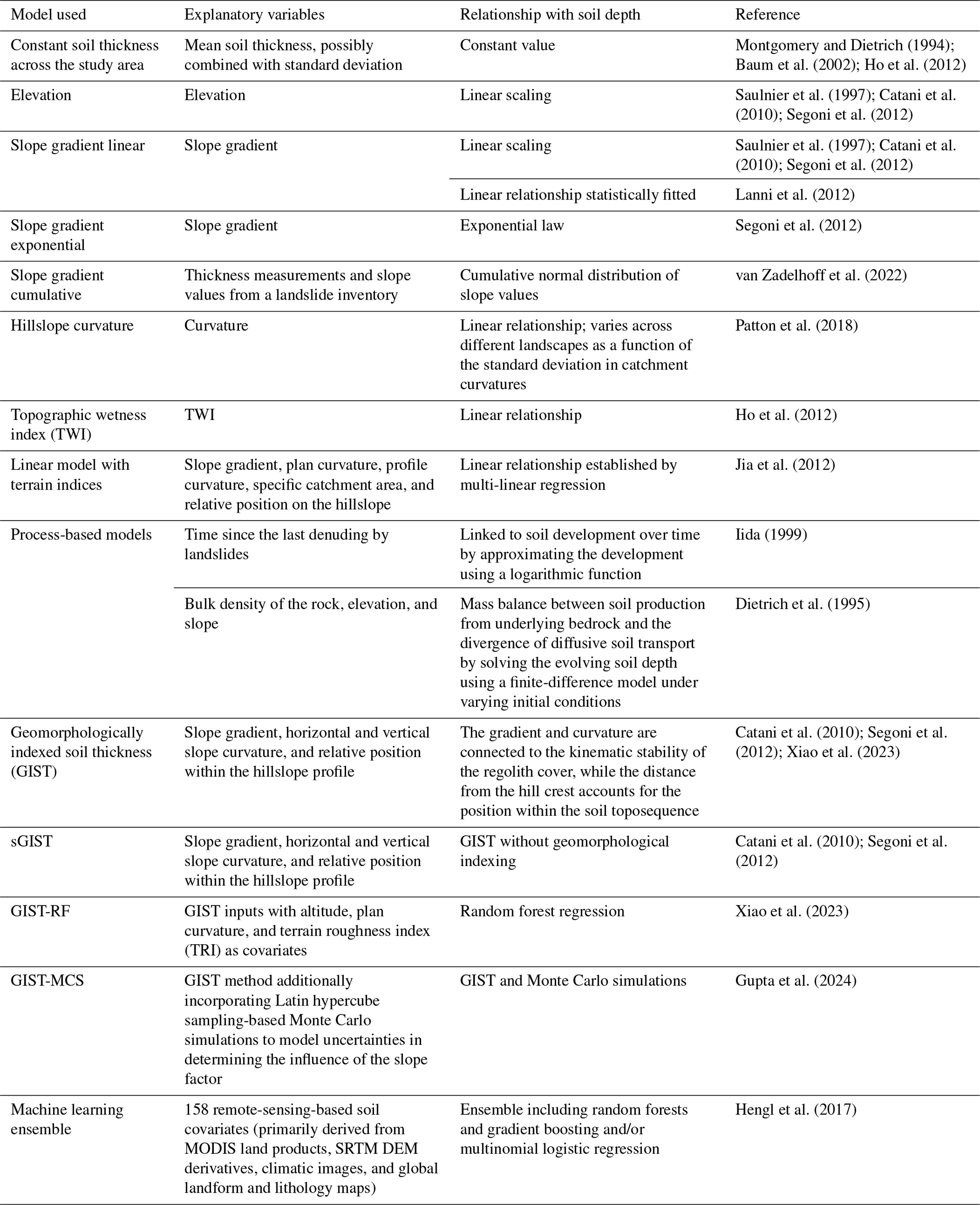
Table 1 gives an overview of models found in the literature for predicting soil thickness, with a focus on those applied in shallow-landslide simulations. The explanatory variables used in these models have informed the choice of covariates for this study. Furthermore, they provide good examples of the model types used to predict soil depth. Most of these models are either deterministic (e.g. Montgomery and Dietrich, 1994; Baum et al., 2002) or probabilistic (e.g. van Zadelhoff et al., 2022).

Montgomery and Dietrich (1994); Baum et al. (2002); Ho et al. (2012)Saulnier et al. (1997); Catani et al. (2010); Segoni et al. (2012)Saulnier et al. (1997); Catani et al. (2010); Segoni et al. (2012)Lanni et al. (2012)Segoni et al. (2012)van Zadelhoff et al. (2022)Patton et al. (2018)Ho et al. (2012)Jia et al. (2012)Iida (1999)Dietrich et al. (1995)Catani et al. (2010); Segoni et al. (2012); Xiao et al. (2023)Catani et al. (2010); Segoni et al. (2012)Xiao et al. (2023)Gupta et al. (2024)Hengl et al. (2017)

Table 1 List with a summary of soil thickness models found in the literature.

The accuracy of the potential landslide thickness is of paramount importance for the performance of slope stability models (cf. Iida, 1999; Larsen et al., 2010; Milledge et al., 2014; van Zadelhoff et al., 2022). Consequently, improving the estimation of landslide thickness is key for enhancing the performance of slope stability models. With the overall aim of developing a model that provides a more accurate prediction of the potential shallow-landslide thickness compared to pre-existing simple models, the four main objectives of this study are the following:

1. to present descriptive statistics on data regarding the thickness of shallow landslides and additional potentially explanatory data from two field inventories in Switzerland;

2. to develop and test new models for predicting the potential thickness of shallow landslides in Switzerland based on ML (random forest (RF) models, generalised additive models (GAMs), and linear regression models (LMs)) using input variables including terrain metrics and vegetation;

3. to evaluate the performance of the developed models using data from the two shallow-landslide inventories;

4. to compare the performance of the developed models with three previously published models that predict shallow-landslide thickness based on altitude, slope, and cumulative slope distribution.

2 Study area

The study area is distributed across Switzerland (Fig. 2), which has a total area of 41 291 km² (FSO, 2021). The Swiss landscape can roughly be divided into the Alps, covering around 58 % of the country; the Central Plateau, covering 31 %; and the Jura, covering 11 % (FDFA, 2023). The Jura mountains in the northwest are mainly characterised by limestones and marls (Pfiffner, 2021; Zappone and Kissling, 2021). The Central Plateau, extending from Geneva towards the northeast, is a molasse sedimentation basin covered by thick Quaternary deposits resulting from the erosion of the Alpine chain (Reynard et al., 2021). With the Helvetic, Penninic, and Austroalpine nappes, the Alps include three major nappe systems. Parts of these nappes can be referred to as pre-Alps (see Fig. 2), which include lower mountain ranges and in the most northern parts even foothills. The alpine nappe piles have led to the amalgamation of very different rock types. These include continental and oceanic basement rocks (granites, gneisses, and schists); shallow-marine carbonates (limestones and marls); deep-marine clastics (sandstones and conglomerates), which locally resulted from turbidites known as flysch deposits; and radiolarian chert (Pfiffner, 2021). Switzerland is characterised by a temperate semi-continental climate that is strongly influenced by its altitude and its complex topography (Fallot, 2021). The mean annual air temperature varies with the altitude, showing 8.5–11.9 °C at 500 m above sea level, 6.2–9.6 °C at 1000 m, and 3.9–7.3 °C at 1500 m over the period from 1981–2010 (Fallot, 2021). The mean annual rainfall increases with altitude, with values from 900–1300 mm for the Central Plateau, and gradually increases from the southern piedmont of the Jura mountains towards the northern side of the Alps where these amounts exceed 2000 mm and reach up to 3000 mm yr⁻¹ or more on the wettest summits in the Central Alps.

3 Materials

3.1 Landslide inventories

This study used reference datasets compiled from two different Swiss landslide inventories. The first dataset (hereafter HMDB), created by Rickli et al. (2016, 2019), is based on a comprehensive database of shallow landslides and hillslope debris flows (WSL, 2024) that occurred between 1997 and 2021. Most of the HMDB records were collected after heavy rainfall events within defined perimeters. The data in this inventory are based on field surveys performed with identical protocols that include relevant variables such as the dimensions of the landslides, site characteristics, and runout characteristics (Rickli and Graf, 2009; WSL and BAFU, 2018). If values could not be measured in the field (e.g. because of terrain changes since the event), the database may contain estimated values that are marked accordingly (Rickli et al., 2016). The location of the landslides is recorded by geographical x and y coordinates of the failure point in the Swiss coordinate system LV95 measured at the upper edge of the scarp. Of the 760 entries in the inventory, 75 comprised measured thickness values and 199 comprised estimated thickness values in the field. These were recorded perpendicular to the original slope surface (T_L in Fig. 1). We were able to estimate the thickness by dividing the recorded landslide volume by the recorded failure area for 435 records. This approach was chosen based on an exchange with the author of the database (Christian Rickli, personal communication, 2023), as the mean landslide thickness in the HMDB is mainly used for the estimation of the failure volume (Rickli et al., 2016). In the end, we had 711 records with thickness values. Since we removed two records with an estimated value larger than 2 m from the dataset, the resulting dataset comprised 709 records.

The second dataset (hereafter KtBE) is based on an inventory created by the office for natural hazards of the canton of Bern (Hählen, 2023) and comprises 519 landslides, 6 of which are also recorded in the HMDB inventory. The landslides in the KtBE inventory were recorded between 2005 and 2021. For the inventory, the failure zones and runout envelopes of shallow landslides were digitised as polygons from orthoimages. The mean thickness of the landslides is derived from expert estimates based on the orthoimages. The author estimated that there is a possible error of between 25 % and 50 % for the thickness (Hählen, 2023). Since only events for which the entire process area could reliably be reconstructed from the orthoimages were recorded, many events in forests or intensively cultivated areas were not included in the inventory. This limits the possibility of making comparisons between landslides within and outside of forests. Four records were filtered out from the dataset because of a missing thickness value or a thickness value larger than 2 m, leaving 515 records in the final dataset.

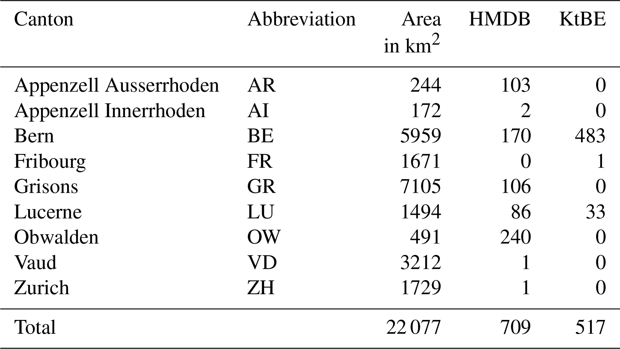
The distribution of the landslide locations across Switzerland (Fig. 2) and the number of landslides per canton (Table 2) are uneven. The fact that the datasets only contain records for 9 of the 26 cantons in Switzerland is caused by not only uneven occurrence of landslides but also differences in the availability of recorded data. While the recorded landslides are distributed across large parts of Switzerland, there is a clear concentration on the northern parts of the Alps and pre-Alps. Locally clustered occurrences were mostly caused by specific extreme precipitation events in combination with unfavourable geological substrata such as flysch or molasse (Reynard et al., 2021; Steger et al., 2022).

.

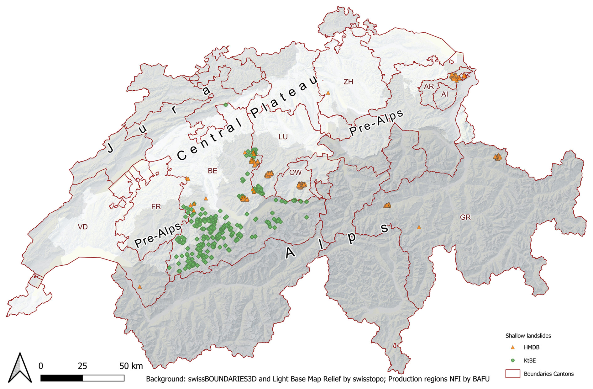
Figure 2 Map of the recorded shallow-landslide locations across Switzerland for the HMDB (orange triangles) and KtBE (green diamonds) datasets. The Jura, Central Plateau, pre-Alps, and Alps are indicated with different shades of grey. Background: swissBOUNDARIES3D (Swisstopo, 2024b), production regions NFI (BAFU, 2020), and light base map relief (Swisstopo, 2024c)

Table 2 Number of recorded landslides per canton in the HMDB and KtBE shallow-landslide datasets.

3.2 Model input data

The following datasets were used as input for the models in this study:

• the light detection and ranging (lidar)-based swissALTI3D digital elevation model (DEM) with a cell size of 0.5 m (Swisstopo, 2023a);

• EU-DEM v1.1 with a cell size of 25 m (EEA, 2016);

• a lidar-based vegetation height model (VHM) with a cell size of 1 m (cf. Schaller et al., 2023);

• a National Forest Inventory (NFI) forest type raster (2018) with a cell size of 10 m, indicating the proportion of coniferous trees (Waser and Ginzler, 2018);

• modelled data on extreme point precipitation (Frei and Fukutome, 2022) with a cell size of 1 km for different return periods (2, 10, 30, 50, 100, 200, and 300 years);

• rock densities across Switzerland in the form of a vector-based dataset (Swisstopo, 2020);

• soil property maps with a cell size of 30 m, providing predictions for clay, sand, and silt contents at 0–30, 30–60, and 60–120 cm (Stumpf et al., 2024);

• the ground cover layer of swissTLM3D (Swisstopo, 2023b);

• topographic catchment areas of Swiss water bodies (BAFU, 2019).

Section 4 explains why these datasets and the derived covariates were included. Note that we used a preliminary version of the soil property maps, kindly provided by the Swiss Competence Center for Soils (CCSol, 2024).

4 Methods

In the first part, we analysed the distributions of the thickness and slope gradients of the landslides in the HMDB and KtBE datasets. We used the R environment for statistical computing (R Core Team, 2022) to calculate the descriptive statistics. These included the minimum, maximum, mean, standard deviation, median, and mean absolute deviation (MAD) for the landslide thickness and slope gradient recorded in the inventories as well as the elevation and slope gradient from the covariates.

The subsequent modelling part is divided into three stages (Fig. 3). In stage 1, intermediate DEM rasters for the subsequent stage were prepared. During stage 2, the data used for the final modelling and analysis stage were prepared. The covariates, such as terrain variables or geology, were derived based on the DEM and other input data. Following this, the covariates were added to the reference data by sampling the generated rasters at the landslide failure points. The analysis and modelling based on the previously prepared dataset were performed in stage 3, including the training of three types of machine learning (ML) models and the application of three simple model types.

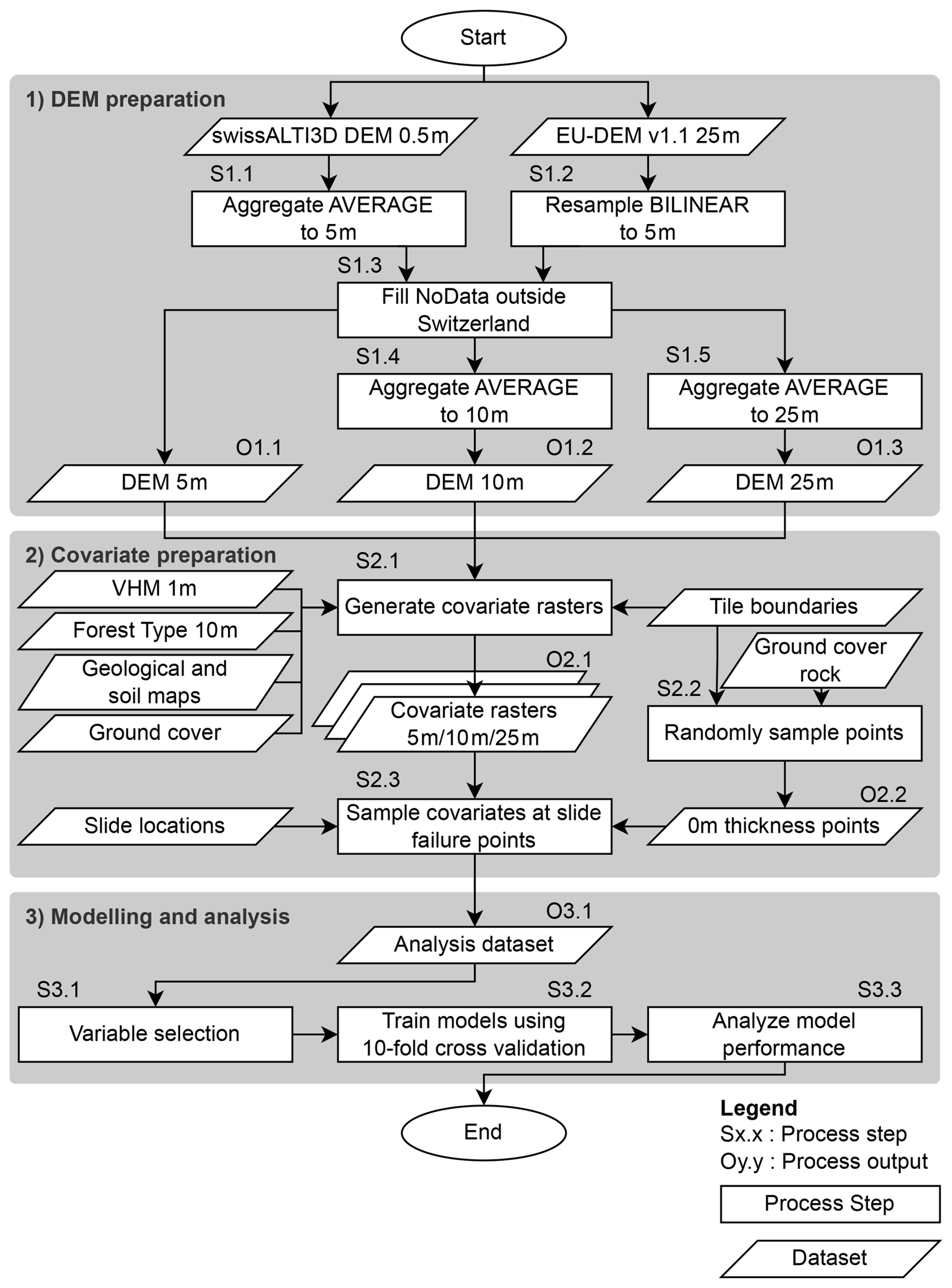
Figure 3 Flowchart of the methodology applied in this study. The three separate grey boxes delineate the (1) DEM preparation, (2) covariate preparation, and (3) modelling and analysis stages.

All three stages were implemented in R. The calculation of some variables was implemented in R using the sf (Pebesma and Bivand, 2023) and terra (Hijmans, 2023) packages. However, the processing of most variables was implemented using System for Automated Geoscientific Analyses (SAGA) GIS (Conrad et al., 2015) via the RSAGA package (Brenning, 2008) or using Geospatial Data Abstraction Library (GDAL) tools (GDAL/OGR contributors, 2021) from R. The code for the entire process can be found in the repository accompanying this study (Schaller, 2025).

4.1 DEM preparation

The covariates for the ML models were calculated as rasters with a cell size of 5, 10, and 25 m (outputs O1.1, O1.2, and O1.3 in Fig. 3). The 0.5 m cell size swissALTI3D DEM was used as input for the terrain-based covariates. The original DEM was first aggregated to a 5 m cell size using gdalwarp with the average function (step S1.1 in Fig. 3). The areas outside the Swiss borders are not covered by swissALT3D. Covariates calculated over a window would lead to incorrect values near the border. Therefore, the areas outside the border were filled using EU-DEM. For this purpose, the original extent of the 5 m DEM was first buffered by 4 km to accommodate the largest radius used in the covariate calculations (step S1.2 in Fig. 3). The areas with no data within that buffered extent were then filled using values from EU-DEM resampled to 5 m using gdalwarp with a bilinear function (step S1.3 in Fig. 3). This filled raster was the primary input for the terrain analysis. The additional DEM rasters with 10 and 25 m cell sizes were derived by aggregating the filled 5 m DEM using gdalwarp with the average function (steps S1.4 and S1.5 in Fig. 3). Although the resampling of EU-DEM introduces a certain error in the elevation values outside the border, we regard this error as an acceptable trade-off for the good data availability and the simplified data preparation process.

4.2 Covariate preparation

4.2.1 Calculating covariate rasters

As can be seen in the overview of the processed variables and their corresponding cell sizes (Table 3), some covariates were calculated for all three cell sizes, while others were only calculated for specific cell sizes. Vector-based input data were rasterised, including the generation of separate $\mathrm{0}/\mathrm{1}$ encoded rasters for categorical variables. The terrain-based covariates calculated from the DEM included metrics commonly used in terrain analysis, hydrology, and geomorphology that were also used in other studies aiming to predict failure or soil depth. To represent the influence of the forest, the VHM was used to calculate statistics on vegetation height, while the NFI forest type raster was used as an indicator of species composition, which can influence the stabilising influence of forests. The rock densities across Switzerland (Swisstopo, 2020) served to represent the underlying lithology. The density of rocks varies based on their chemical composition and the structure of their minerals (from crystalline to amorphous) (Zappone and Kissling, 2021). Each entry in the dataset is assigned to 1 of the 21 defined lithological groups and shows the expected range in which the mean bulk density of the local lithology varies (Swisstopo, 2020). For an overview of the lithology groups and densities, refer to the visualisations in Zappone and Kissling (2021) and the documentation included in Swisstopo (2020) or its visualisation in the Swisstopo web map portal (Swisstopo, 2024a). Similarly, the soil property maps were used to test their influence on landslide depth. The modelled data on extreme point precipitation (Frei and Fukutome, 2022) were used as a proxy variable assuming that locations with potentially extreme rainfall amounts would experience increased erosion and landsliding activity, which would lead to reduced soil cover. The swissTLM3D ground cover layer (Swisstopo, 2023b) was tested as a categorical covariate and was used to identify areas with rock cover.

(Swisstopo, 2023a)(EEA, 2016)(Swisstopo, 2023b)Frei and Fukutome (2022)Schaller et al. (2023)Waser and Ginzler (2018)Zappone and Kissling (2021)Stumpf et al. (2024)

Table 3 Variables explored as covariates for the machine learning models along with their input data and the tools used for their processing.

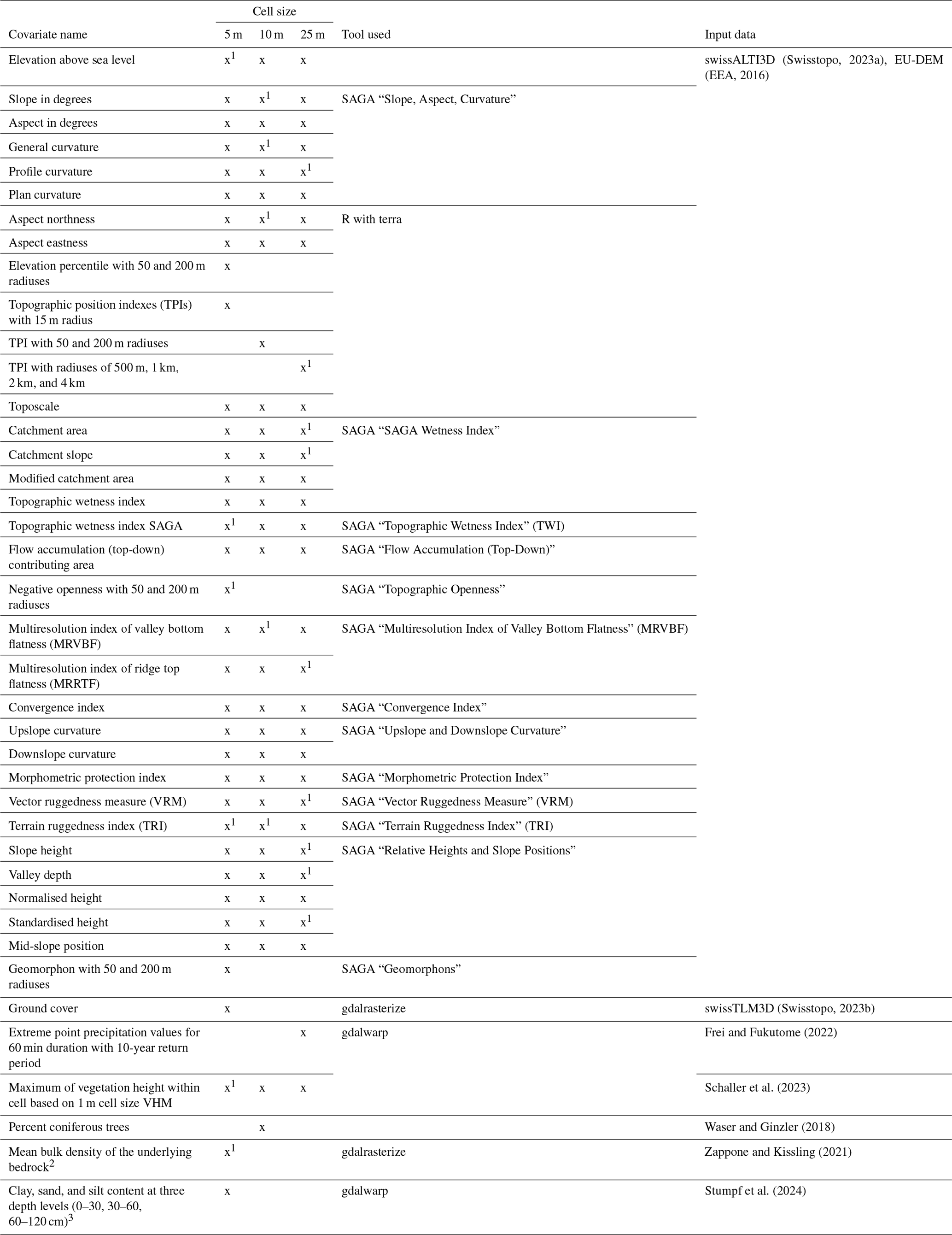
¹Variables and cell size used in the final ML models. ²Sampled directly from the original vector data. ³Sampled directly on the original 30 m cell size raster.

To optimise the calculation of covariates for the entire area of Switzerland, the processing of the covariates was parallelised (step S2.1 in Fig. 3). For this purpose, Switzerland was divided into tiles based on aggregated catchments. The tiles based on catchments ensure that the values calculated for hydrological covariates are correct within the catchment area. We used the pre-defined aggregation level of the topographic watershed dataset (BAFU, 2019), which defines watersheds with a size of approx. 150 km². These correspond to a tile size with acceptable processing times while keeping the number of tiles at a manageable level. For the actual processing, the extents of the catchments were buffered by 500 m (5 and 10 m rasters) or 4 km (25 m rasters) to ensure data availability for covariates calculated with window sizes that go beyond the catchment border. Only the covariate values within the catchment borders were used for further processing since the values outside the border may be incorrect. Note that variables connected to hydrology were not calculated based on the original DEM raster but a sink-filled version of the DEM generated using the SAGA GIS tool “Fill Sinks” based on the method by Planchon and Darboux (2002).

4.2.2 Sampling covariate values

After calculating the covariate rasters, we prepared the dataset for the subsequent modelling and analysis stage. This was achieved by merging the event data from the inventories with the covariate values by sampling the cell values at the failure point of the landslides (step S2.3 in Fig. 3). In the case of the HMDB dataset, the reported coordinates of the failure point were used directly. For the KtBE dataset, only the event envelopes were available as input. Therefore, the failure point was approximated based on the envelope polygon. First, the elevation for the vertices was determined by sampling the 5 m cell size DEM. Following this, the x and y coordinates of the approximate failure point were calculated as the average for the corresponding coordinates of the vertices with an elevation equal to or higher than the 95th percentile of the elevation of all vertices of the envelope polygon.

The inventories only contained entries for locations with actual landslides and therefore a sufficient soil thickness. To better reflect the fact that landslides cannot occur in areas with bare rock, additional points with a landslide thickness of 0 m in rocky areas were added to the analysis dataset (step S2.2 in Fig. 3). The points were randomly generated within the areas marked as rock or loose rock in the ground cover layer of the swissTLM3D landscape model (Swisstopo, 2023b) using the spatSample() function of the terra package in R (Hijmans, 2023). The points were generated separately for each dataset and only within the rock signatures in the catchments containing slide events. After generation, the points were manually checked for plausibility using the SWISSIMAGE orthoimages (Swisstopo, 2024d). The number of generated points actually included in the datasets is proportional to the percentage of the catchments covered by the rock signature, namely 34 points for the HMDB dataset (4.1 % rock cover) and 53 points (9.7 % rock cover) for the KtBE dataset.

4.3 Modelling and analysis

4.3.1 Models and covariate selection

We tested three different types of ML models for predicting the potential failure thickness of shallow landslides. The R Classification And REgression Training (caret) package (Kuhn, 2008) was used to fit these models. Due to the promising performance of random forests (RFs) in other studies, our development efforts were mainly focused on RF models (Breiman, 2001), implemented using the ranger package (Wright and Ziegler, 2017). In addition, we tested linear regression models (LMs) using the built-in lm function of R and generalised additive models (GAMs) using the mgcv package (Wood, 2011), which allowed us to model non-linear relationships. We chose these model types to evaluate whether they could achieve performance similar to RF models while maintaining explainability (James et al., 2021).

All three model types were trained using the same input data and validation procedures. The covariates included in the models were chosen based on a combination of exploratory analysis, inputs from the literature (especially the works listed in Table 1), and expert knowledge of the authors (step S3.1 in Fig. 3). The exploratory analysis included test-fitting RF models with both the HMDB and the KtBE datasets to determine variable importance and attempts at automatic variable selection using recursive feature elimination. The inputs from the literature and the expert knowledge of the authors influenced the overall selection of the tested covariates. From the pool of candidates, we aimed to select covariates with high importance, whose combination resulted in good model performance, while keeping the number of covariates and, therefore, model complexity low. At the same time, we tried to balance the inputs from the test fittings with the expert-based input, leading to the following choices of covariates:

• aspect_nness_10, northness of the aspect calculated as cosine(aspect) at a 10 m cell size;

• curvature_10 and curvature_profile_25, general curvature at a 10 m cell size and profile curvature at a 25 m cell size, as calculated by the SAGA module Slope, Aspect, Curvature;

• h_5, altitude above sea level sampled at a 5 m cell size;

• mrrtf_25, multiresolution index of the ridge top flatness at a 25 m cell size;

• mrvbf_10, multiresolution index of valley bottom flatness at a 10 m cell size;

• openness_neg_200_5, negative openness calculated with a radius of 200 m at a 5 m cell size;

• rhob_m, mean bulk density of the local lithology;

• slope_10, slope gradient in degrees at a 10 m cell size;

• slope_height_25, standardised_height_25, and valley_depth_25, slope height, standardised height, and valley depth at a 25 m cell size calculated by the SAGA module Relative Heights and Slope Positions (Böhner and Selige, 2006);

• tpi_500m_25 and tpi_4km_25, topographic position indexes 500 m and 4 km with a window size at a 25 m cell size;

• tri_r5_5 and tri_r5_10, terrain ruggedness index with a radius of five cells for 5 and 10 m cell sizes;

• twi_5, catchment_area_25, and catchment_slope_25, topographic wetness index, catchment area, and catchment slope at 5 and 25 m cell sizes, as calculated by the SAGA module SAGA Wetness Index (Böhner et al., 2002; Böhner and Selige, 2006);

• vhm_max_5, maximum vegetation height at a 5 m cell size;

• vrm_r5_25, vector ruggedness measure with a radius of five cells at a 25 m cell size.

Additionally, three simple models for predicting soil depth were applied as a comparison to the three ML models. The first two models that we adapted were proposed by Saulnier et al. (1997) and predict soil thickness, which is often used as a proxy for landslide thickness. They use a predicted soil depth based on either elevation (hereafter Simple-Z) or slope gradient (hereafter Simple-S) by applying a linear interpolation based on the minimum and maximum values in a set of reference data. The third method used for comparison, proposed by van Zadelhoff et al. (2022) (hereafter SFM), also uses the slope gradient to predict soil depth. However, to account for the shallow soils on steep slopes, the method derives the soil thickness from a log-normal distribution and multiplies it by a correction factor, which is a function of the slope gradient. For the Simple-Z model, the elevation sampled at a 5 m cell size was used to train the model. For the Simple-S and the SFM models, the slope sampled at a 10 m cell size was used since it showed the best fit with the slopes at the failure point recorded in the inventories.

4.3.2 Training and validation

Separate models were trained for the HMDB and KtBE datasets, resulting in 12 models overall (step S3.2 in Fig. 3). Both datasets were split into training data (80 %) and validation data (20 %). All models were trained using 10-fold cross-validation (James et al., 2021). The built-in caret functions were used for the RF model, GAM, and LM. Custom cross-validation methods were written for the Simple-Z, Simple-S, and SFM models. The structure of the RF model, GAM, and LM was automatically determined by caret during the training process.

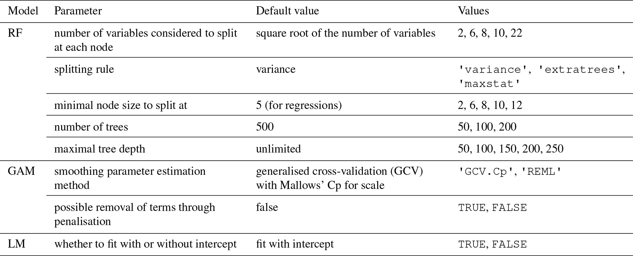
The hyper-parameters of an RF model can significantly influence model performance (Huang and Boutros, 2016; Probst et al., 2019). Therefore, the training of the RF model was combined with a hyper-parameter tuning leveraging a modified version of the tune-grid functionality included in the caret package. The function performs a grid search over a defined set of parameters and values (see Table 4). Similarly, the standard hyper-parameters for GAM and LM available in caret were tuned. The final RF model showed clear differences in the chosen hyper-parameters. The HMDB-trained model used the split rule “extratrees”, a minimum node size of 2, 2 variables to split at, and 100 trees with a maximum depth of 50. The KtBE-trained model used the split rule “maxstat”, a minimum node size of 10, 8 variables to split at, and 50 trees with a maximum depth of 150. For the GAMs of both datasets, the REML method was used for smoothing parameter estimation. The KtBE-trained model was fitted with possible penalisation of terms (i.e. each term can potentially be removed from the model during fitting by adding an additional penalty), while the HMDB-trained model was fitted without. For the LM, the hyper-parameter tuning resulted in a fit without intercept for the HMDB-trained model and a fit with intercept for the KtBE-trained model.

Table 4 Parameters and values used for tuning the hyper-parameters for the random forest (RF) model, generalised additive model (GAM), and linear regression model (LM).

Performance measures were calculated based on the application of the trained models to the respective validation data in order to assess model performance (step S3.3 in Fig. 3). In addition, the models trained with the HMDB dataset were cross-applied to the KtBE validation data and vice versa to evaluate the transferability across datasets.

We used the MAE of predicted landslide thickness versus landslide thickness from the inventory as the primary performance assessment measure, which was calculated as

$$\begin{array}{}\text{(1)}& \mathrm{MAE}={\displaystyle \frac{\mathrm{1}}{n_{\mathrm{slides}}}}{\mathrm{\Sigma }}_{i=\mathrm{1}}^{n_{\mathrm{slides}}}|y_{{\mathrm{Actual}}_i}-y_{{\mathrm{Predicted}}_i}|,\end{array}$$

where MAE is the mean absolute error of the landslide failure thickness, $y_{{\mathrm{Actual}}_i}$ is the landslide failure thickness in metres for landslide i according to the inventory, $y_{{\mathrm{Predicted}}_i}$ is the landslide failure thickness in metres for landslide i predicted by the model, and n_slides is the total number of landslides in the reference data.

Additionally, we calculated the coefficient of determination R² to judge how good the fit between the predicted and actual data is:

$$\begin{array}{}\text{(2)}& R^{\mathrm{2}}=\mathrm{cor}(y_{\mathrm{Actual}},y_{\mathrm{Predicted}}{)}^{\mathrm{2}},\end{array}$$

where R² is the coefficient of determination, y_Actual is the landslide failure thicknesses in metres according to the inventory, and y_Predicted is the landslide failure thickness in metres predicted by the model.

5 Results

5.1 Statistical properties of landslide inventories

The distributions of the landslide thickness in the HMDB and KtBE datasets are very similar, with mean and median values that lie close to each other (see Table 5). The histogram of the landslide thickness (Fig. 4a) shows that 90 % of the landslides had a thickness smaller than or equal to 1 m in the HMDB and KtBE datasets, and both show peaks at 0.5 and 1 m. This is especially the case for the KtBE dataset, which also shows additional small peaks at 1.5 and 2 m landslide thickness. In both the HMDB and the KtBE datasets, landslides mainly occurred at slope angles above 15°, with a tendency for the number of occurrences to increase with the slope angle and a sharp decrease above 40° (Fig. 4b). Half of the landslides occurred above 36° in the HMDB dataset and above 31° in the KtBE dataset. Almost no landslides occurred on slopes with a slope angle higher than 55° or below 15°. Visual verification of the landslides outside these boundaries using orthoimages and maps confirmed that the failures are plausible. The landslides above a 55° slope angle (HMDB: n=4) were all located in forested areas, and most landslides below 15° (HMDB: n=16, KtBE: n=5) were located at a transition between flat and steep terrain, such as a terrace or a road. The comparison of the recorded slope values with those from the covariates sampled at 5 m cell size showed slightly lower mean and median values for the HMDB dataset and very similar values for the KtBE dataset. The elevation range where shallow landslides occurred, as well as its distribution, is similar in both datasets (Table 5). In the distribution of the landslide thickness over the slope classes (Fig. 5), the KtBE dataset shows a slight tendency towards decreasing landslide thicknesses and lower variance with increasing slope steepness. The HMDB dataset shows a similar, albeit even weaker, tendency towards such a decrease and no discernible pattern in the variance.

Table 5 Summary statistics including the total number of records (n); n within forests; and the minimum, median, median absolute deviation (MAD), mean, standard deviation (SD), and maximum for important characteristics of shallow landslides derived from the landslide inventories and from covariates derived from swissALTI3D (Swisstopo, 2023a). Note that lower sample sizes result from missing values in the inventory.

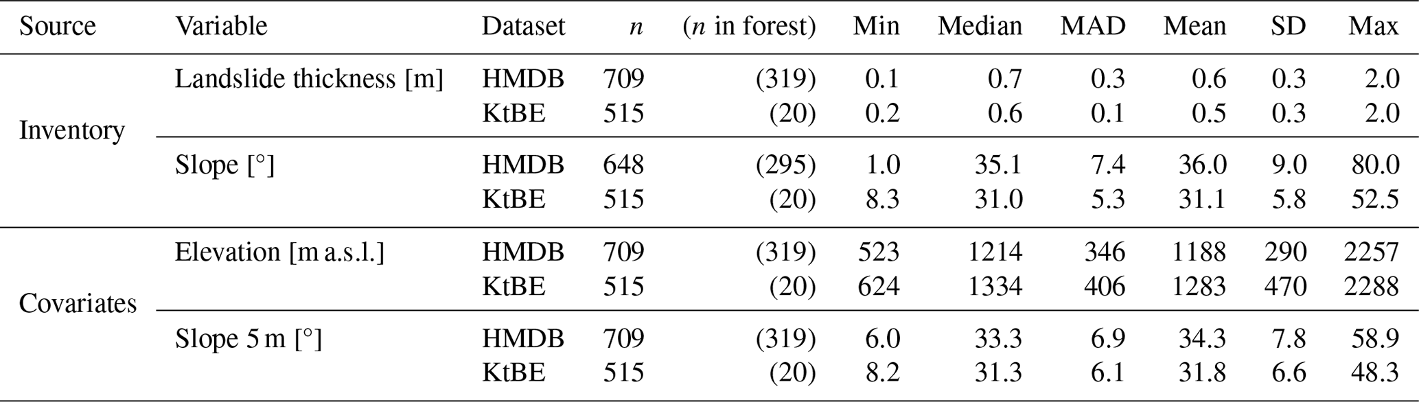
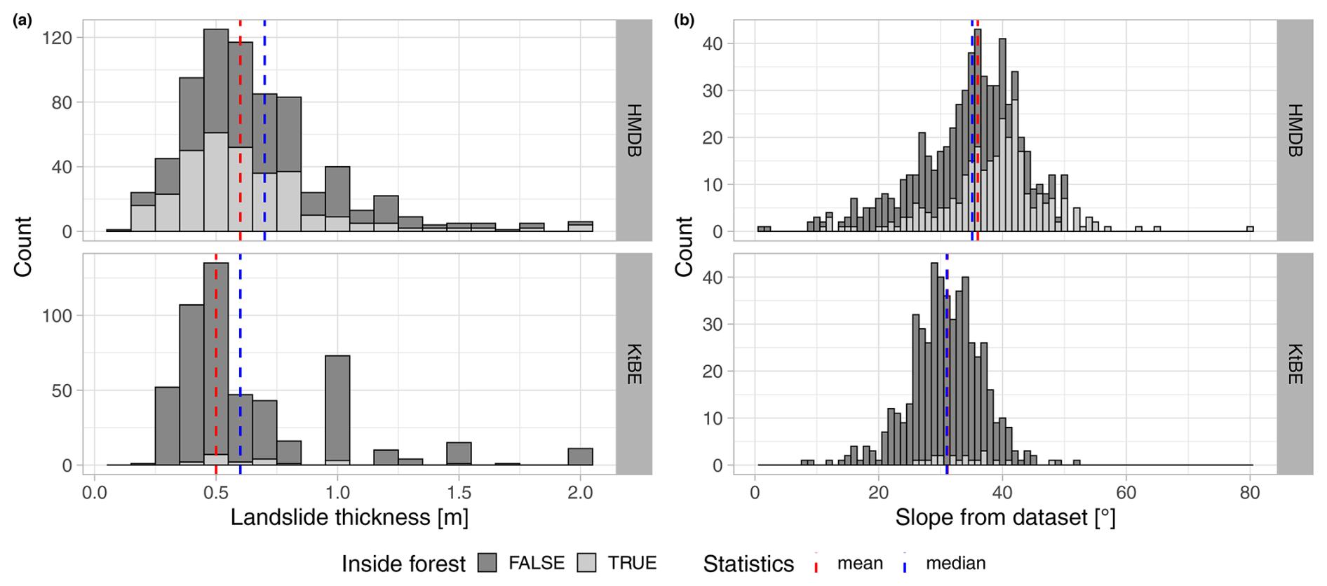
Figure 4 Histograms showing the distribution of (a) the landslide thickness and (b) the mean slope values in the release areas recorded in the HMDB (upper row) and KtBE (lower row) datasets.

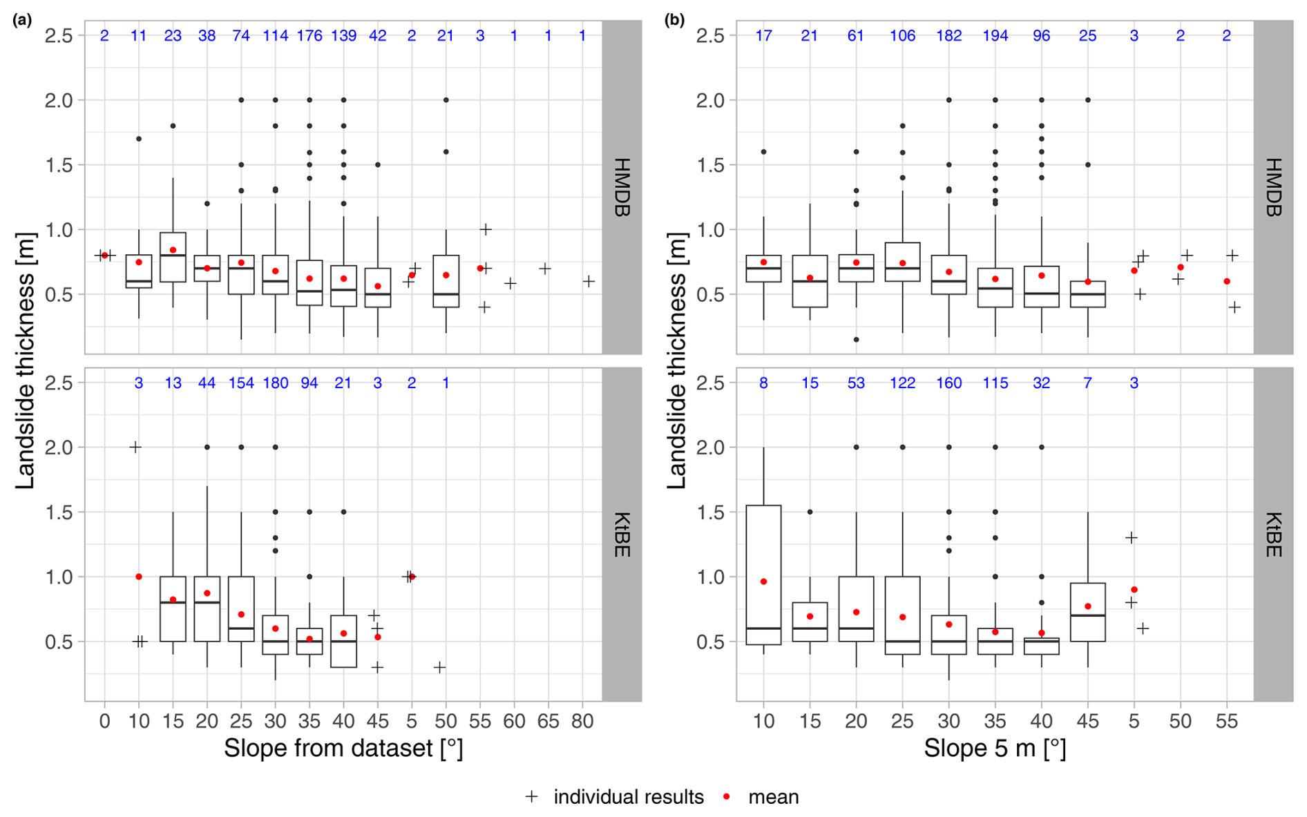
Figure 5 Box plots showing the distribution of the landslide thickness over slope classes based on (a) the reported slope for the different datasets and (b) the slope values sampled at 10 m cell size. The red dots represent the mean value, while the blue numbers show the number of records per slope class. Individual cross-shaped points are shown for classes with fewer than five data points.

5.2 Modelling results

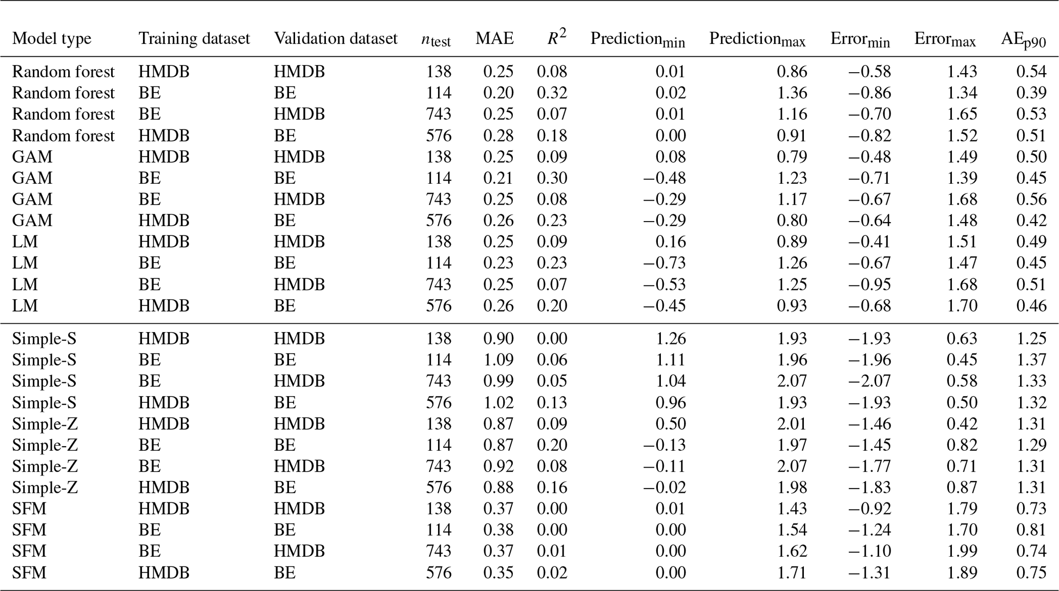
Overall, the RF models performed best, with an MAE of 0.25 m for the HMDB dataset and 0.20 m for the KtBE dataset (see Table 6). While the MAE values of the GAMs and LMs are comparable for the respective datasets, their R² values tend to be lower than those of the RF models. Furthermore, both the GAMs and the LMs show some outliers with negative prediction values of up to −0.73 m. The Simple-Z and Simple-S models clearly show worse performance, with MAE values exceeding 1 m. The SFM model achieved MAE values of 0.37 m for HMDB and 0.38 m for KtBE. When comparing the performance between the datasets, the models for the KtBE dataset performed slightly better than the HMDB-trained models. The results for the cross-application are variable. In most cases, MAE values were comparable to those of the model trained with the same dataset, with differences between 0 and 7 cm for the ML models and between −7 and 9 cm for the simple models.

Table 6 Performance of the trained models. Results are shown for the application of the respective dataset to the validation data and for the cross-application to the other dataset. n_test denotes the number of records in the validation data. Prediction_min and Prediction_max correspond to the minimum and maximum predicted values, while Error_min and Error_max correspond to the minimum and maximum errors. AE_p90 denotes the 90th percentile of the absolute error.

The data points of the measured vs. ML-predicted landslide thickness are located closer to the identity line when compared to the three simple models (see Fig. 6). However, all three models showed a tendency to slightly overestimate lower landslide thicknesses and distinctly underestimate higher thicknesses. The Simple-S model tended to overestimate the landslide thickness clearly across the entire range. The Simple-Z model showed a similar tendency but with a higher variance. The SFM model also exhibited a high variance but with predictions closer to the identity line. In particular, the added points with 0 m landslide thickness showed high variances in all three of the simple models.

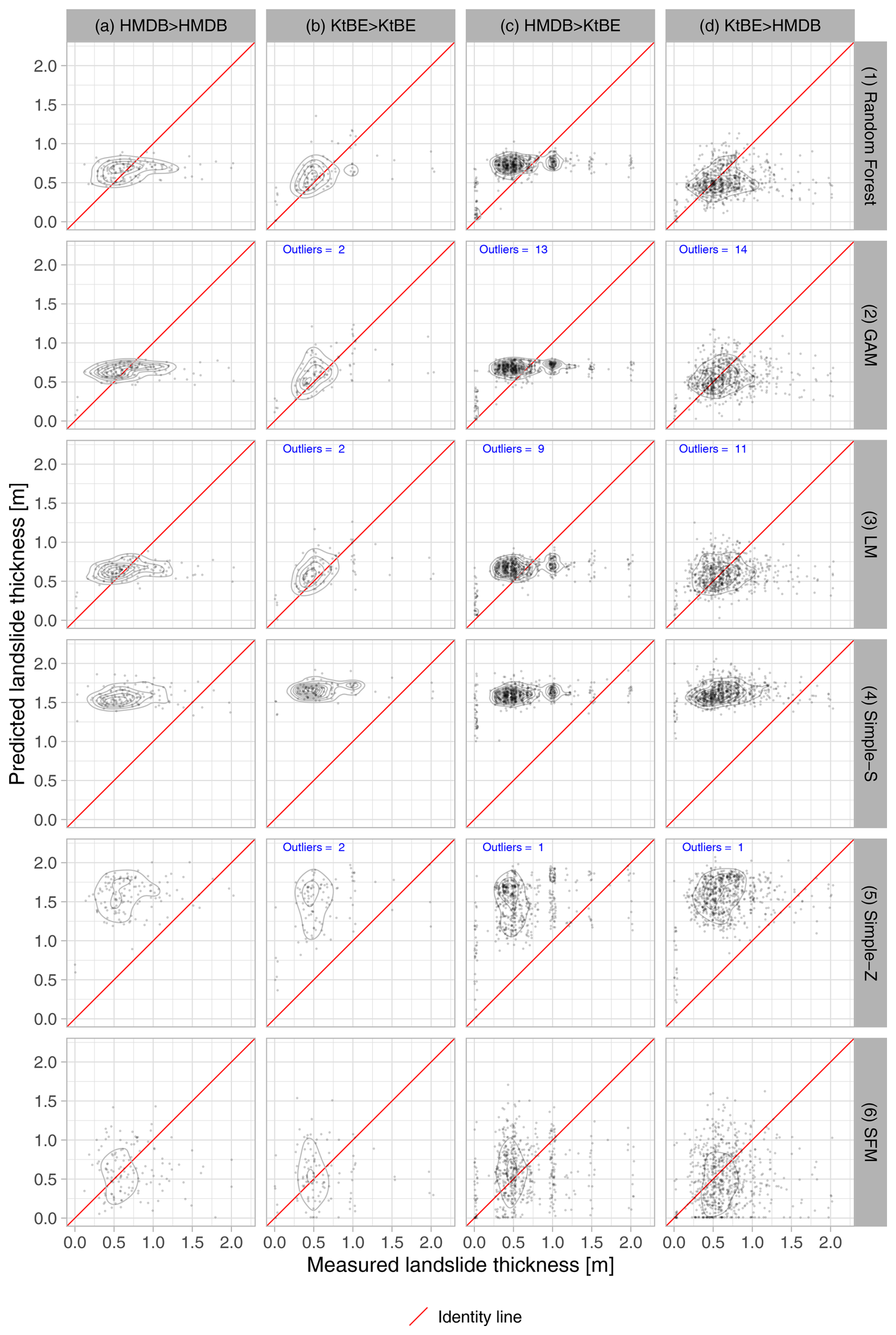
Figure 6 Scatter plots showing the measured vs. predicted landslide thickness differentiated by model type (rows) and dataset (columns): (a) model trained and tested with the HMDB dataset, (b) model trained and tested with the KtBE dataset, (c) model trained with the HMDB dataset and tested with the KtBE dataset, and (d) model trained with the KtBE dataset and tested with the HMDB dataset. The diagrams have 2D kernel density contours in the background and an identity line in red. Where present, the blue text denotes the number of outliers outside the display range of the plots.

The distribution of the residuals per slope class (Fig. 7) was similar for most slope classes where training and validation data stem from the same dataset. Some classes, like e.g. the 40° class of the HMDB dataset, show higher variance. The simple models generally also had higher variances than the ML models. Looking at the cross-application of the models (Fig. A1 in Appendix A1), there were evidently more outliers and higher variances across all slope classes. In particular, the 15° class of the HMDB-trained models applied to the KtBE data consistently showed high variances.

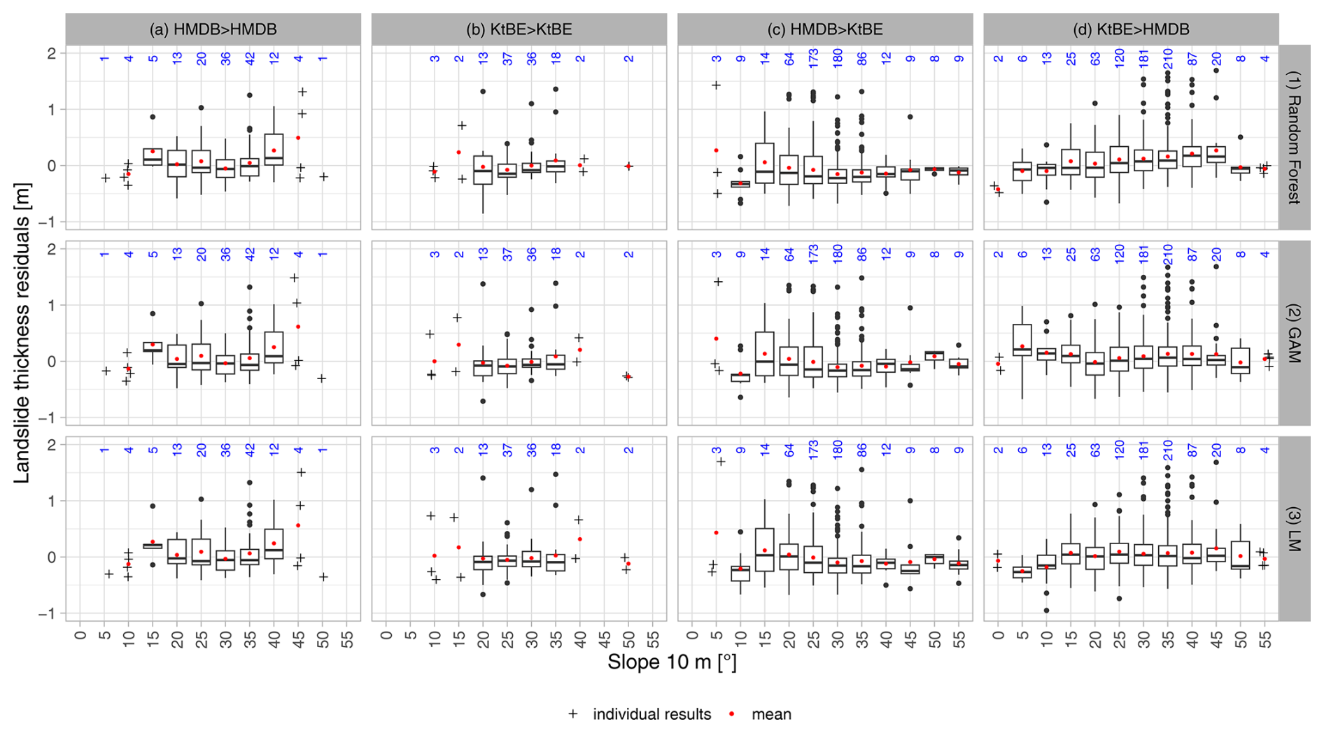
Figure 7 Box plots showing slope classes sampled at 5 m cell size vs. the residuals of the predicted landslide thickness for the best three models differentiated by model type (rows) and dataset (columns; see caption of Fig. 6 for details). The red dots represent the mean value, while the blue numbers show the number of entries per slope class. Individual cross-shaped points are shown for classes with fewer than five data points. For readability, those that occurred above the 55° slope gradient class are not displayed here.

The analysis of the variable importance of the ML models showed clear differences between the models. However, the variable elevation, terrain roughness index at 10 m cell size, mean density of the local lithology, negative openness, and multiresolution valley bottom flatness are found more often among the top-ranked ones (compare Fig. A2 in supplementary materials). The hyper-parameter tuning resulted in a reduction in the MAE of up to 2 cm for certain models. The chosen parameters were the same across most of the datasets.

6 Discussion

6.1 Landslide inventories

The slope values recorded in the HMDB and KtBE landslide inventories (cf. Fig. 4) largely match the ranges found in the literature, with reported values from 5 to 35° (Guzzetti et al., 2008a), 20 to 35° (Meier et al., 2020), 22 to 40° (Dahl et al., 2010), and 19 to 50°, with predominant values from 25 to 45° (Rickli and Graf, 2009).

Larsen et al. (2010) compared data on landslide thickness from several landslide inventories located across the globe, some of which showed peaks around 0.5, 1, and 2 m, similar to the ones observed in the HMDB and KtBE inventories. Particularly in the KtBE dataset, the observed peaks are a possible bias of the expert estimations. For the KtBE dataset, the errors in the landslide thickness were estimated to be 25 % to 50 % (Hählen, 2023). In general, the data quality of the inventory data is crucial for its suitability for ML. A contrasting example is the Swiss national register of natural hazard events (“StorMe”), which is maintained by the Federal Office for the Environment (FOEN) and the cantons (Burren and Eyer, 2000). The distribution of the landslide depth of a selection of 2988 shallow landslides recorded in StorMe (Fig. 8) shows similar peaks but in a much more pronounced manner. We also attribute these peaks and the gaps in between to rough estimates by many different experts performing the recording of event characteristics in the field. We tested the StorMe data for possible use in this study. However, the anomalies in the landslide thickness distribution together with other data quality issues, like missing or unrealistic values, led to the exclusion of the dataset. This illustrates that initiatives like the HMDB and the acquisition of more high-quality data play a key role in obtaining the input data necessary for future ML-based modelling.

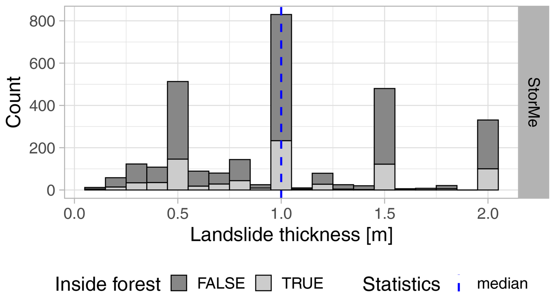
Figure 8 Histogram showing the distribution of the landslide thickness recorded for 2988 shallow landslides in the Swiss national register of natural hazard events (StorMe).

6.2 Model performance

Among the three ML models tested, our study focused on RF because of its potential. The LMs and GAMs served as reference models with different properties. RF models can flexibly capture non-linear relationships and interactions between variables and covariates (Breiman, 2001; James et al., 2021). However, their complex model structure and ensemble nature hinder model explainability and result interpretation (Breiman, 2001; James et al., 2021). LMs have the advantage of a transparent model structure that is simple to implement but cannot capture non-linear relationships (James et al., 2021). GAMs are an extension of LMs that allow us to model non-linear relationships by fitting smoothing functions to the explanatory variables (Hastie and Tibshirani, 1990; James et al., 2021). However, they are more susceptible to overfitting (Wood, 2011). In addition, interactions must be explicitly specified for LMs and GAMs, since they are not captured automatically (James et al., 2021). The results from the model tests reflect some of the different model properties and, overall, confirmed the potential of the ML models for predicting the potential failure thickness of shallow landslides.

The ML models clearly outperformed the two simple models based on the elevation and slope gradient proposed by Saulnier et al. (1997). However, it has to be noted that those models were originally intended to be used in smaller areas like single catchments with more uniform terrain, whereas our application covers a much larger area in Switzerland with more diverse terrain conditions. Although the SFM model proposed by van Zadelhoff et al. (2022), calibrated with the values from the inventories, produced better results, the RF model still yielded MAE values that were 20 % to 44 % lower. While the ML models exhibited low errors, they all tended to underestimate higher landslide thickness values. We attribute this to the low number of records with a landslide thickness of more than 1 m in the datasets used for model training. The cross-application of the ML models showed that they are mostly transferable between the HMDB and KtBE datasets. One limiting factor might be the spatial and temporal hierarchy in the HMDB data resulting from the fact that most of the data were recorded in perimeters after defined heavy rainfall events. However, tests showed no significant signs of spatial autocorrelation in the model predictions. Another limiting factor may be the missing events in forests or in intensively cultivated areas not recorded in the KtBE inventory. Nevertheless, there appears to be enough similarity in the distributions of the landslide thickness over the slope classes and the covariates in both datasets to conclude that the models are transferable. This is supported by an additional test with a cross-application of the HMDB-trained model to the StorMe dataset, which showed a clear decline in performance. We attribute this mainly to the distinctly different distribution of the landslide thickness in the StorMe inventory with the dominant peaks at 0.5, 1, and 2 m. This indicates a limited generalisability of the trained models, although this may also be due to differences in data quality.

Although comparability is limited due to differences in the study area extents and the use of soil depth landslide thickness instead of soil depth as the target variable, our results show similar tendencies to comparable studies. Catani et al. (2010) applied two simple models based on the elevation and slope proposed by Saulnier et al. (1997), along with the geomorphology-based GIST model in the Terzona catchment (24 km²) in Italy. The Simple-Z and Simple-S models performed the worst, with MAE values of 0.94 and 0.54 m, while the GIST model had an MAE of 0.11 m. Subsequently, Segoni et al. (2012) applied the same models in the Armea catchment (37 km²) in Italy. The Simple-Z and Simple-S models again performed worse, with MAE values of 0.78 and 1.03 m compared to an MAE of 0.23 m for the GIST model. An additional model linking the soil depth to the slope using an exponential function showed an MAE of 0.45 m but tended to give unrealistically low prediction values. Xiao et al. (2023) applied the GIST model and the random-forest-based GIST-RF model to generate soil depth maps in a section along the Yangtze River in Wanzhou County (27 km²), where soil depth ranges from 0 to 40 m. The MAE values of 10.6 m for the GIST showed that the original model cannot deal with the complex geological settings and high variability in soil depth at the study site. However, the GIST-RF model showed an MAE of 3.52 m, demonstrating the potential for improvement through ML techniques. Gupta et al. (2024) applied GIST, GIST-MCS, and GIST-RF models in a study assessing soil thickness along three important roads (673 km²) in the Joshimath region (Indian Himalaya). The GIST, GIST-MCS, and GIST-RF models showed MAEs of 3.94, 2.86, and 1.64 m, thus further confirming the potential of GIST-RF.

The results of the ML models are promising. The RF model showed the overall best performance, with the best fit and no undesired outliers. The performance of the GAMs and LMs was comparable, although they had an overall worse fit and showed undesired outliers (especially negative ones). The partial effect plots for the GAMs showed that the degree of smoothing is low or close to zero for most terms. This is, at least in part, a result of the automatic estimation of the smoothing functions performed by caret, which does not allow any manual intervention. We expect that the GAMs could be improved by manually building a model with individualised terms and smoothing functions. Overall, additional tests and optimisation may be advisable. In particular, we would expect the inclusion of additional records with a landslide thickness between 1 and 2 m to improve the model performance. The hyper-parameter tuning only yielded improvements that did not exceed a reduction in the MAE by 1 cm. However, the difference of up to 2 cm between some of the hyper-parameter combinations for the RF models shows that hyper-parameter tuning is generally worthwhile. The results of the hyper-parameter tuning for the RF models also showed tendencies that are mostly in line with the findings reported by Probst et al. (2019). Additional model variants with and without additional points with 0 m landslide thickness in rock signatures have been explored. However, while the addition of the points did increase the overall MAE of the ML models by about 1 to 5 cm, most of the R² values clearly improved. At the same time, the points with 0 m landslide thickness also influenced the mean of the predicted values. For the ML models and the SFM model, there was a decrease of 2.4 to 6.4 cm in the overall mean of the predicted values. For the Simple-S and Simple-Z models, the mean of the predicted values increased by 13.1 to 21.6 cm. Due to this influence and given the large variance of the predictions for the 0 m thickness points, it is still not clear to us whether the addition of the points is recommendable. The scheme used for random sampling in space could potentially introduce a bias and class overlap (i.e. overlap between conditions associated with occurrences of events and pseudo-absences), which may be mitigated by adopting a uniform sampling approach (Da Re et al., 2023).

6.3 Covariate selection

The selected covariates in the ML models mostly describe the terrain and its geomorphology. This shows parallels to models aiming to predict soil depth in general based on geomorphology (Catani et al., 2010; Xiao et al., 2023). The elevation, slope, TWI, curvature, and aspect included in our covariates were also identified by Zweifel et al. (2021) as important causal factors of shallow landslides in grassland regions of Switzerland. In addition, the inclusion of covariates in the vegetation and underground are worth mentioning. The influence of the vegetation (especially the forest) was realised by including the maximum of the VHM. This variable consistently showed higher importance for the models trained with the HMDB data compared to the KtBE-trained models. This may be due to the low number of landslides within the forest present in the KtBE data. While the high importance of the maximum of the VHM suggests a significant influence of the forest, the NFI forest type raster with the proportion of coniferous trees was not included in the final model. The reason was the very low or even negative importance values, suggesting a lack of relationship with the target variable, which could be a result of the distribution of the landslides inside the forest. The geological substratum was included by the mean local density of the underlying bedrock serving as a proxy for the lithology. While the importance of lithology varied significantly between the different model types and dataset combinations, it was high enough to warrant inclusion in the model. The covariates on soil properties were ultimately not included in the final model. On the one hand, the importance of the clay, sand, and silt content at the different depths varied considerably from negative importance to moderately important depending on the dataset. We tested several covariate selections, including different combinations of reasonably important soil property variables and the mean bedrock density. While some of these combinations showed an MAE close to or even slightly better than the final selection, they also showed lower R² values. In addition, adding up to nine different variables would have increased the model complexity considerably. Together with the uncertainties related to the soil property data, this led to the decision not to include any soil property covariates in the final model.

A variant of the ML models including the rainfall amount for a duration of 60 min for an extreme point precipitation event with a 10-year return period as an additional variable was also explored. The results, however, were almost identical to the model without this additional variable. We speculated a priori that this variable might be related to soil thickness due to an erosion effect, but this is apparently not the case or not detectable. Aiming for a model with less complexity, we finally opted to exclude this variable.

6.4 Uncertainty

Although the performance of the model is promising, it is subject to uncertainties, which are a challenge in natural hazard modelling and prediction. Uncertainty quantification is critical for improving the reliability and interpretability of predictive models, particularly in applications that inform risk management and mitigation. While various methods exist for quantifying uncertainty, they differ significantly across disciplines and model types, with no universally applicable solutions for machine learning models (Beven, 2018; Jalaian et al., 2019; Simmonds et al., 2022). Unlike classical statistical models such as linear regression, which offer established confidence interval formulas, machine learning approaches often lack analogous tools, creating additional challenges for systematic uncertainty evaluation (Jalaian et al., 2019). In this study, we did not apply uncertainty quantification due to the heterogeneous nature of the tested models and the inherent difficulties in quantifying uncertainties in both reference and covariate data. These data constitute a significant source of uncertainty, as inaccuracies in inputs propagate through the models, ultimately influencing predictions (Simmonds et al., 2022). Addressing these data uncertainties is crucial for enhancing the robustness of ML-based models and should be prioritised in future research, similar to the work of Meinshausen (2006) and Wager et al. (2014), who provided confidence intervals for RF.

The main uncertainties in the covariate data lie in the soil, geological substratum, and forest type datasets. The soil and geological substratum cannot, for the most part, be measured directly, making data subject to uncertainties based on model assumptions and mapping precision. Similar to the model in our study, the values in the tested soil property maps were predicted using a quantile regression forest (Meinshausen, 2006) based on sparse field measurements and a large number of covariates derived from remote sensing (Stumpf et al., 2024). The resulting predictions are already subject to a considerable degree of uncertainty, especially due to the 30 m cell size and the high local heterogeneity in soil properties. In the geological data, uncertainties stemming from different surveyors and methodologies cannot be ruled out. This is exemplified by the discontinuities in the data stemming from different map sheets in the original data on bedrock and unconsolidated deposits from the GeoCover dataset (Swisstopo, 2023c) used in preliminary tests. The bulk density dataset of local lithology explicitly attempts to quantify variability and uncertainty by including percentile values of the density distributions (Swisstopo, 2020; Zappone and Kissling, 2021). While this approach enhances transparency, the uncertainty still reflects natural variability within lithologies, errors in physical property measurements, and sparse sampling coverage (Zappone and Kissling, 2021). Forest type data, modelled using RF and neural networks using remote sensing data (Waser et al., 2017), are similarly subject to uncertainty. Significant deviations from the national forest inventory, particularly in the underestimation of broadleaved trees, highlight the limitations of current methods (Waser et al., 2017). The authors primarily attributed these deviations to errors in the input image data rather than the classification approach itself (Waser et al., 2017).

Uncertainties in the field inventory data used to train the models also influenced the accuracy of model predictions. Positional errors in the failure points, e.g. due to imprecise GPS measurements, can result in inaccurate sampling of covariates, reducing model reliability. This issue is partially mitigated by the averaging effects of the larger cell sizes and windowed calculations used for the covariate rasters. Additionally, errors in estimating landslide thickness present a challenge, as these inaccuracies can render datasets unsuitable for ML applications. For example, the limitations of the StorMe dataset due to unreliable thickness estimates highlight the necessity for improved field data protocols tailored to ML requirements.

The uncertainty in the model results is also largely influenced by the choice of model type, training data, and covariates used during the training process (Jalaian et al., 2019). Different combinations of training records and covariates can lead to significant variability in the structure and outputs of the RF models, GAMs, and LMs used. For instance, cross-validation introduces a random factor that can result in variability, particularly when models are trained on small datasets. This variability highlights the need for systematic sensitivity analyses to identify robust covariate combinations that optimise model performance. Moreover, the selection process revealed numerous covariate combinations with similar performance metrics, suggesting a potential for overfitting or underutilising critical variables (cf. Merghadi et al., 2020). Given that optimal covariate combinations may vary depending on cell sizes, input datasets, and model types, future studies should explore adaptive methods for covariate selection that are tailored to specific data and model contexts. This would align model configurations more closely with the specific characteristics of the study area.

7 Conclusions

In this study, we presented an ML-based approach to predict the potential thickness of shallow landslides. The new machine learning models consistently performed at least 20 % better when comparing the MAE to simple models based on slope gradient and elevation. We conclude that the selected set of covariates, including metrics on terrain, geomorphology, vegetation, and lithology, is a suitable basis for predicting shallow-landslide thickness using ML. Considering the overall performance and the lack of outliers in the predictions, we consider the RF model to be the most accurate approach to generate improved inputs for slope stability models. For future work, we plan to adapt this study's RF model, which is built for predictions on single sample points, for the generation of rasters covering large extents. Additionally, the model can be further developed, especially by improving the input dataset with additional field data, by testing variants with additional sample points and sampling schemes for locations with 0 m landslide thickness and by further refining the selection of covariates.

Appendix A: Additional material

A1 Detailed results

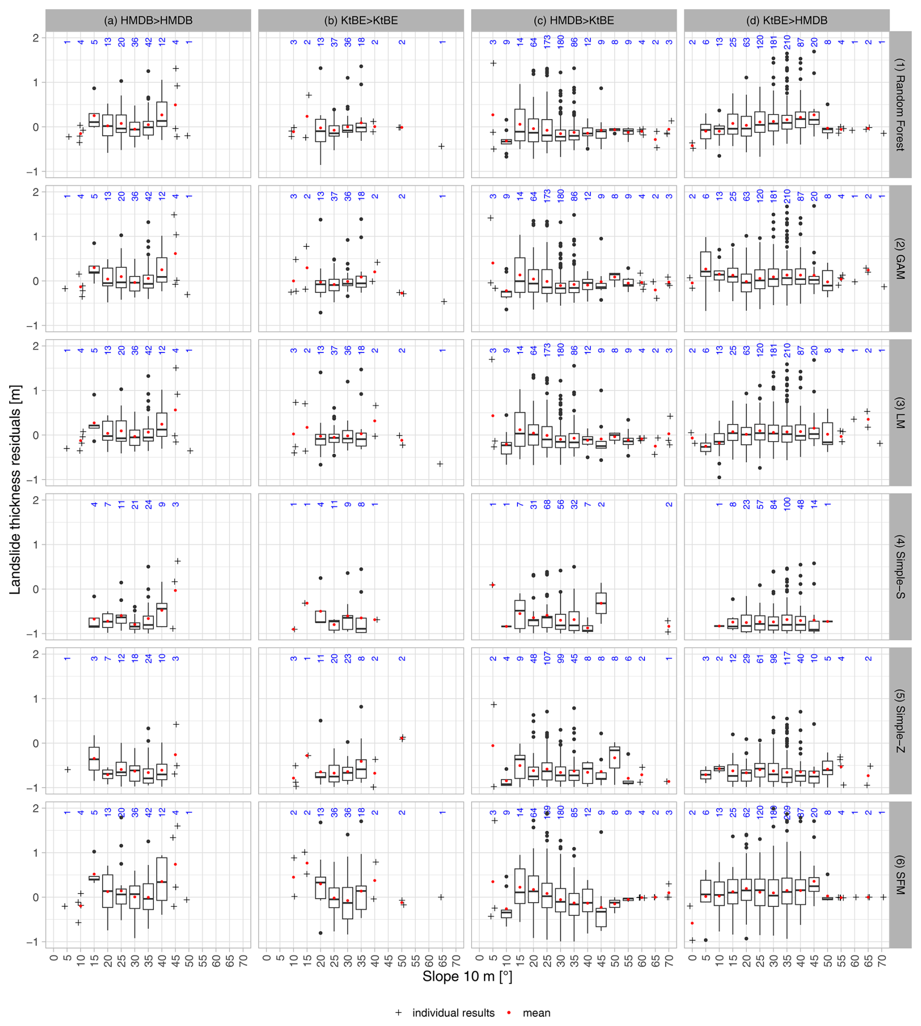
Figure A1 Box plots showing slope classes sampled at 5 m cell size vs. the residuals of the predicted landslide thickness for all models differentiated by model type (rows) and dataset (columns): (a) model trained and tested with the HMDB dataset, (b) model trained and tested with the KtBE dataset, (c) model trained with the HMDB dataset and tested with the KtBE dataset, and (d) model trained with the KtBE dataset and tested with the HMDB dataset. The red dots represent the mean value, while the blue numbers show the number of entries per slope class. Individual points are shown for classes with fewer than five measurements.

A2 Variable importance and model tuning

Variable importance values were extracted for the ML-based models (Fig. A2). The values of the RF model and LM were extracted from the overall result of the 10-fold cross-validation result. Since no meaningful overall values could be extracted from the GAM fit, the importance values from the best model were extracted. The results show that there are differences in the importance of the individual variables depending on the dataset and the model. Nevertheless, several variables are more often among the top-ranked variables, including the elevation, the terrain roughness index at 10 m cell size, the mean density of the local lithology, the negative openness, and the multiresolution valley bottom flatness.

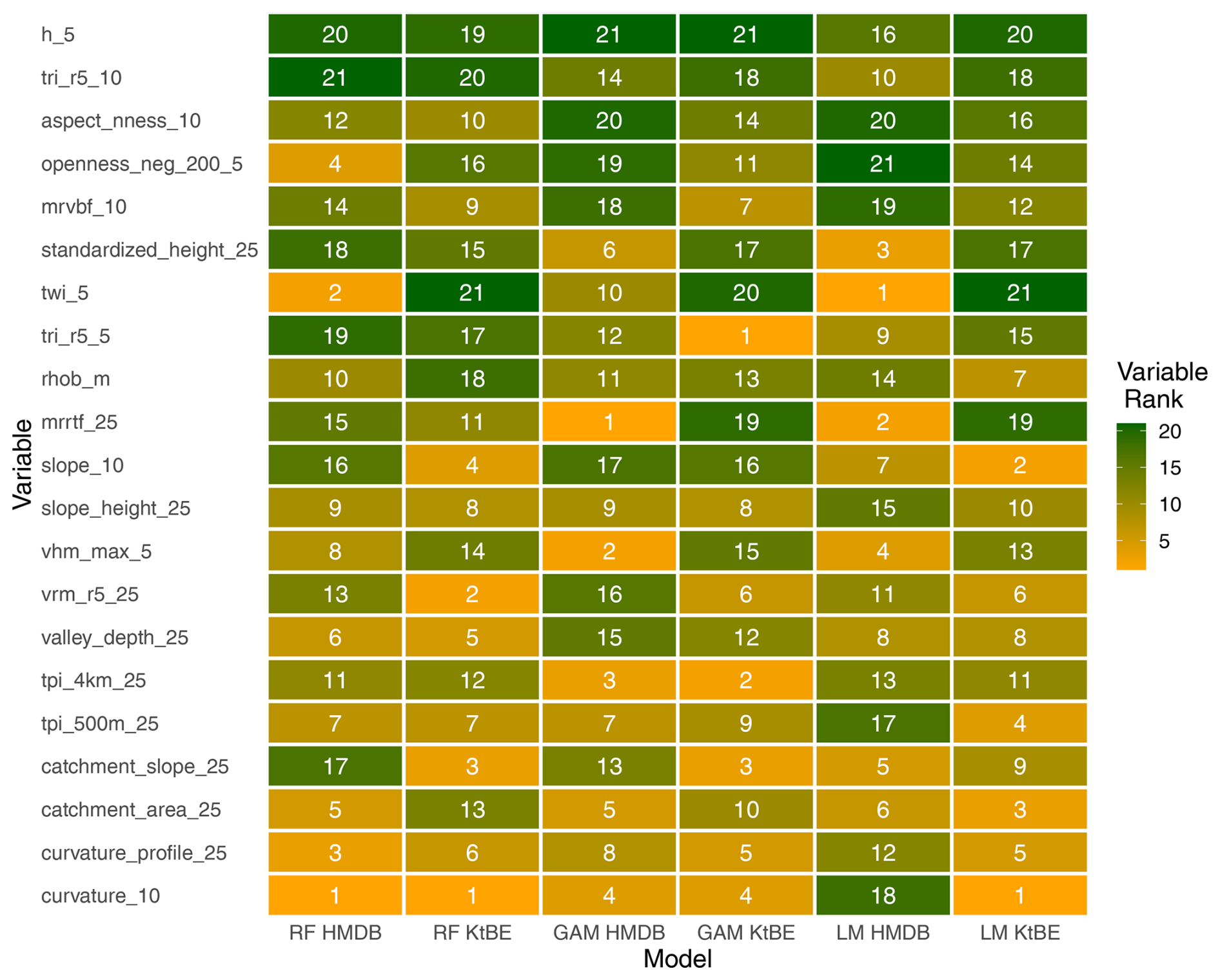
Figure A2 Heatmap showing the overall variable importance extracted from 10-fold cross-validation for the RF model and LM and the importance of the best fit for the GAM. The number in the cells and their colour correspond to the importance rank of the variable within the model, with 21 (green) being the most important variable and 1 (yellow) being the least important variable. The variables are sorted by the sum of the ranks of each row.