Capture of near-critical debris flows by flexible barriers: an experimental investigation

This study addresses the key issue of the interaction between debris flows and flexible barriers based on small-scale experiments for which both the flowing mixture and the barrier were designed to achieve similitude with real situations in Alpine environments. The considered debris consisted of a large solid fraction mixture with large and angular particles, flowing down a moderately inclined flume and resulting in near-critical flows, with a Froude number in the 0.9–2 range. The flexible barrier model consisted in 3D printed cables and net. The flow characteristics, evolution and deposition after contact with the barrier as well as the deformation and the loading experienced by the barrier were addressed varying the flume inclination and released mass. Four different interaction modes between the flow and the barrier are identified increasing the flow kinematics. A model based on the hydrostatic pressure assumption reveals relevant for estimating the total force exerted on the barrier when all the released material is trapped. This force doubles in case there is barrier overflow.

1 Introduction

Debris flows threaten people and assets in mountainous regions (Prakash et al., 2024), and capturing them with barriers is one of the most effective protection strategy (Piton et al., 2024). Over the last decade, a growing number of articles have focused on the interaction between debris flows and both rigid and flexible barriers (see e.g. the reviews by Poudyal et al., 2019; Vagnon, 2020; Kwan et al., 2024). The change in flow dynamics in the barrier vicinity and the loading exerted by the flow on the barrier have been widely addressed mainly based on numerical simulations and experiments at both small-scale and real scale (Albaba et al., 2019; Lam et al., 2022; Ng et al., 2023; Kim et al., 2023; Yune et al., 2023; Choi et al., 2024, among others). Interestingly, a few field measurements, i.e. at real scale and involving a naturally initiated and propagating debris flow, are now available (notably Wendeler et al., 2019; Nagl et al., 2022, 2024), but they remain rare because they require the construction of costly structures and the waiting for significant debris flows, while ensuring that the measurement system continues to function properly in these harsh environments. Our understanding of the reality of debris flow impact against structures is thus still limited and strongly influenced by lab experiments and numerical simulations. In this experimental work, we seek to explore the interactions between flexible barriers having a realistic mechanical behaviour and debris flows having features as similar as possible to that of Alpine events, i.e. surges of mixtures of grain, clay and water with high solid content and a flow regime close to that observed in the field.

A key dimensionless number driving the various regimes of impact with obstacles such as barriers is the Froude number Fr computed as (Faug, 2015, 2021; Laigle and Labbé, 2017):

$$\begin{array}{}\text{(1)}& Fr={\displaystyle \frac{U}{\sqrt{\cos \mathit{\theta }g{h}_{\mathrm{f}}}}}\end{array}$$

with U the velocity of the flow front [m s⁻¹], θ the channel inclination [°] (note that for mild slope, e.g. for θ<15°, $\cos \mathit{\theta }>\mathrm{0.96}\approx \mathrm{1}$ and is usually ignored in the equation), g the gravitational acceleration [m s⁻²], h_f the front thickness (hereafter referred to as the “depth”) measured perpendicular to the flume bottom.

The Froude number of debris flows observed in the field is variable depending on the flowing material and channel characteristics. Many references dealing with debris flows in Alpine environments suggest Froude numbers ranging from 0.5 to 2.4 (Costa, 1984; Hungr et al., 1984; Jacquemart et al., 2017; Wendeler et al., 2019). This typical range was recently confirmed by McArdell et al. (2023), Lapillonne et al. (2023), and by Nagl et al. (2024) based on direct and accurate monitoring of 35 debris flows at the Illgraben torrent (Switzerland), 32 debris flows at the Réal torrent (France) and 45 debris flows at the Gadria torrent (Italy), respectively.

Debris flows with Froude numbers >2–4 exist in nature, but well documented cases appear to correspond to particular contexts. Based on a direct monitoring on the Mt Sakurajima volcano, in Japan, Watanabe and Ikeya (1981) reported Fr ranging within 1.0–2.7. Theses values relate to flows referred to as “lahars” in which volcanic ashes induce a lubrication effect resulting in flows faster than usual debris flows. Mostly supercritical surges were also measured in the peculiar catchment of the Jiangjia Gully in China (Hu et al., 2013; Guo et al., 2020, 2024), typically in the 1.5–3.5 range, with some surges >4. Nevertheless, comparison with other catchments for which data from mud-flows and debris flows monitoring are available reveal that the Jiangjia Gully experiences rather fast debris flows (Phillips and Davies, 1991; Lapillonne et al., 2023; Guo et al., 2024). Consistently, based on a specific flow velocity estimation approach, Prochaska et al. (2008) reevaluated previous field observations concerning debris flows and reached the conclusion that Fr rarely exceeds 3.5, an upper bound already visible in the data compiled by Phillips and Davies (1991). Froude number exceeding 4 are sometimes mentioned in the literature. One of the most frequently cited very high Fr value originates from Fink et al. (1981) who back-computed the features of two surges in the very steep Pine Creek (gradient up to 30°) on the Mount St. Helens. The velocity of the two surges was reconstructed from deposits in bends and resulted in a Froude number >8 for a super fast (15–31 m s⁻¹) and very big surge (with estimated peak discharge =2800–3400 m³ s⁻¹) in a very steep reach (gradient =17–30°). This surge had the features of lahars and its Froude number decreased down to ≈2 further downstream where the gradient was 4°. Although fast and shallow debris-flow surges resulting in high Froude numbers can be reported, also in case of very diluted mud-flows (Yune et al., 2013; Kim et al., 2023), they should be considered peculiar and rather exceptional as related to specific conditions in terms of flowing material characteristics and steepness in particular.

Among the numerous works dedicated to the investigation of the impact of debris flow on structures, the vast majority nonetheless considered supercritical flows (i.e. Fr>1), with Fr ranging from ≈2.5 to >10. Some of these concerned rigid obstacles (Vagnon and Segalini, 2016; Shen et al., 2018; Ng et al., 2019; Kim et al., 2023, among others) and others focused on flexible barriers either based on numerical or analytical models (Li et al., 2020; Song et al., 2021; Kong et al., 2022) or on experiments (Bugnion et al., 2012; Canelli et al., 2012; Ashwood and Hungr, 2016; Tan et al., 2019; Xiao et al., 2023; Berger et al., 2024). On the contrary, debris flows with a Fr<2.5 have been much less considered when dealing with mitigation structures (but see Scheidl et al., 2013, 2023; Ashwood and Hungr, 2016; Chehade et al., 2021; Kong et al., 2021; Song et al., 2023). In the end, it appears that most of the published findings which serve as basis for improving design methods of mitigation structures concern supercritical to highly supercritical flows. As yet suggested by Hübl et al. (2009), it can be considered that models in relation to the flow-barrier interaction have globally been developed on an input data range which does not comply with the most frequently observed debris flows type in Alpine areas. This difference in Froude number results in a difference in loading regime on the barrier. Indeed, many authors have evidenced that above a Froude number of ≈1.4, the loading exerted by a granular flow onto an obstacle was dominated by inertia forces, which relate to the flow velocity, and that, below this value, the loading on the barrier was mainly dominated by gravity forces, associated with the depth of the intercepted material (Tiberghien et al., 2007; Laigle and Labbé, 2017; Wendeler et al., 2019; Huang and Zhang, 2022). In other words, the difference in Fr between most research conditions and what is observed in nature leads to an excess in the attention on the influence of the flow velocity, which has consequences on the knowledge as for the way the flow accumulates, deposits and overflows the structure and more generally interacts with it. There is thus a vital need for an in-depth investigation of the flow-barrier interaction while considering debris flows with a Froude number closer to that in most frequent real Alpine environment cases, i.e. $\mathrm{0.5}<F_r<\mathrm{2}$, in particular in view of improving the design of mitigation structures such as flexible barriers.

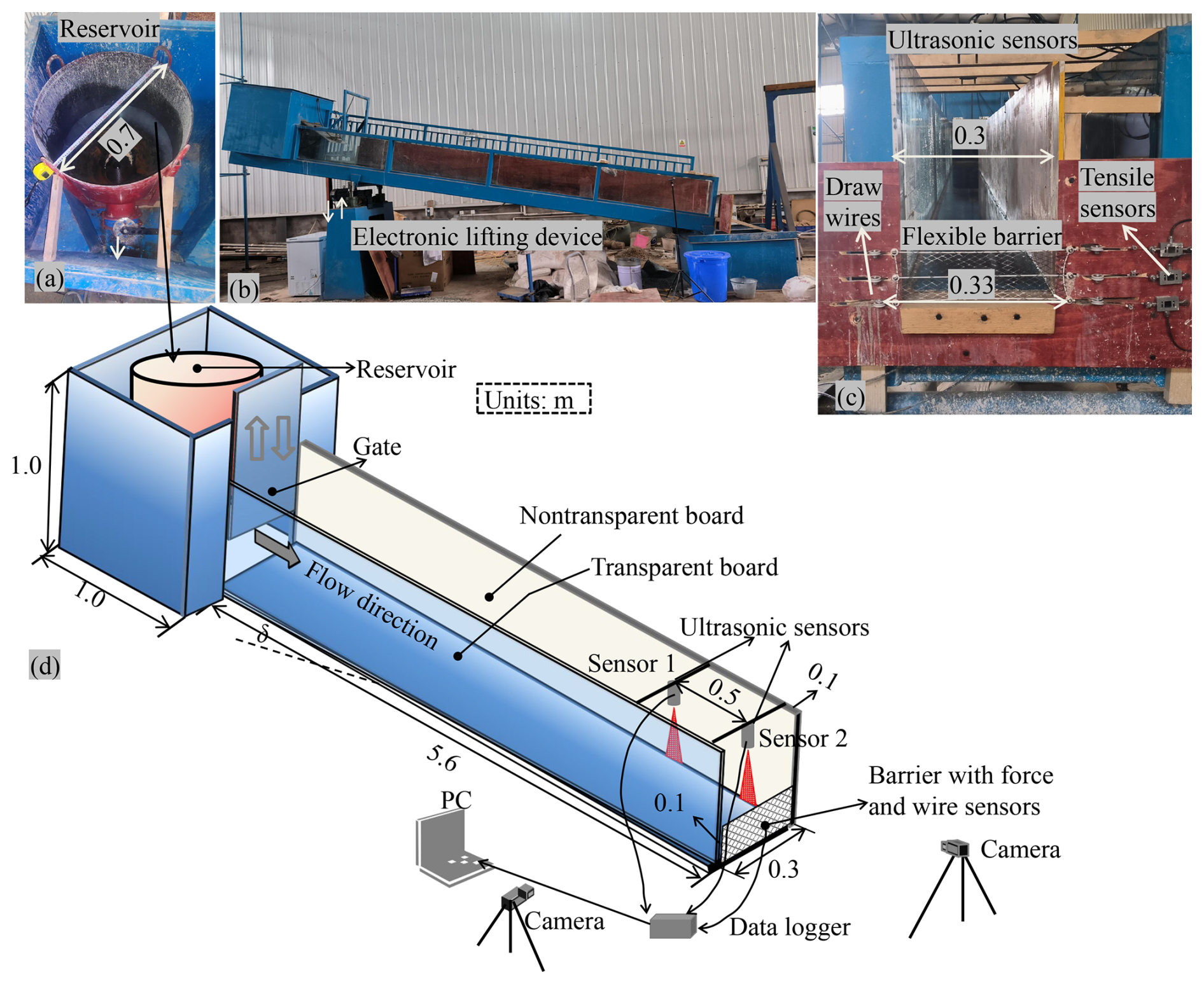
Figure 1 Experimental facility: (a) reservoir for initiation, (b) side view of the whole flume, (c) frontal view of the flexible barrier model and (d) sketch of the flume model.

The design of flexible barriers intended to intercept debris flows is classically conducted by modelling the loading it experiences as a combination of a static component on its lower part and a dynamic one above (Wendeler, 2008; Ng et al., 2012; Ferrero et al., 2015; Sun and Law, 2015; Song, 2016; Tan et al., 2019; Berger et al., 2021). The former corresponds to the loading exerted by the material deposited upstream the barrier (also referred to as “backfill” or “dead zone”) and it is modelled as an hydrostatic pressure along the deposit depth. The latter component corresponds to the action due to the flowing material and is computed as an hydrodynamic loading accounting for the debris flows velocity and density and for an empirical dynamic pressure coefficient of 2 for granular flows and in the 0.7–1 range for viscous flows (according to Berger et al., 2021). Different scenarios are accounted for in design recommendations, in particular in terms of dead zone height (i.e. non-flowing area where the material deposited), barrier overflow, number of surges with consequences on the respective contribution of these two components on the barrier total loading. As most of the research conducted up to now concerned high Fr values, findings from the literature mainly concern high velocity flows, and limited attention was paid to the static component associated with the deposited material.

All in all, this study concerns near-critical debris flows (i.e. with Fr=0.9–2), and involves flume experiments where flexible barriers in mechanical similitude with the real scale are used for the first time to the best of our knowledge (small scale barriers are usually unrealistically stiff or flexible as explained later). The study is conducted varying the flume inclination and the mass of released material while considering different barriers. A particular focus is placed on the flow description and on the barrier loading at rest, which can be assimilated to the static loading component considered in design practices. The paper is organised as follows: (i) the Material and Methods Section describes the flume setting, how the debris flow material was prepared and experiments were run, as well as the experimental plan. (ii) The Results Section describes the features of the approaching flows, the interaction modes and the barrier loading. A discussion and a conclusion close the paper.

2 Materials and methods

The laboratory experiments were carried out in an inclined flume at the extremity of which the flexible barrier was secured. A coarse and saturated mixture of grains, clay and water was released from a reservoir into the flume and subsequently reached the barrier. The characteristics of the flowing material and of the flexible barrier were designed to meet similitude criteria, at a $\mathrm{1}/\mathrm{40}$ scale. Various equipments were used to characterize the flow propagation and the flexible barrier response with time.

2.1 Flume

The flume was 5.6 m in length, 0.3 m in width and 0.5 m in height and had one lateral transparent wall (Fig. 1). The flume bottom and lateral wall were flat and smooth. Its inclination could be varied from 10 to 20°.

To prevent from consolidation, a mixing facility into a cylindrical reservoir was installed at the upstream extremity of the flume (Fig. 1a). The debris flow material was mixed by mixers in this reservoir and then released in the flume by manually opening the butterfly valve underlying the reservoir.

2.2 Flowing material

The flowing material consisted of a mixture of sand gravel, clay and water consistent with real debris flows (76 % of grains of various sizes, 24 % of water and clay) with a solid volume fraction of 73 % (solid mass fraction of 87 %). The characteristics of the mixture (wide grain size distribution, clay into the interstitial fluid, water content <50 %) were determined to mimic coarse-grained debris flow with a high solid fraction commonly found in Alpine region while considering a $\mathrm{1}/\mathrm{40}$ scale ratio (driving for instance the maximum grain size that would be 0.8 m at prototype scale) and meeting similitude requirements thanks to the Froude number, (i.e. Fr≈0.9–2).

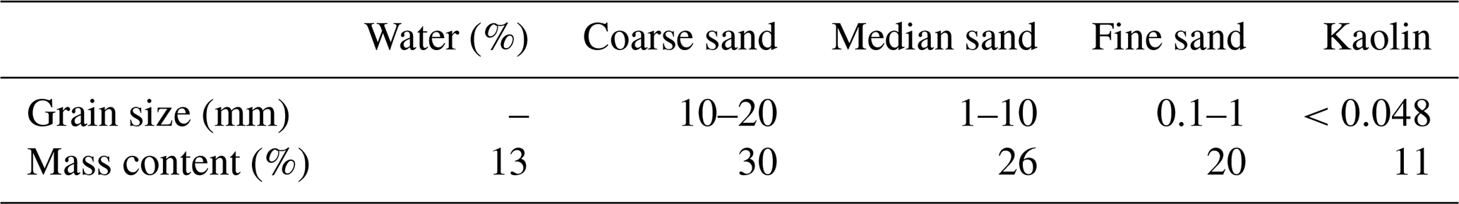
Preliminary tests were conducted to determine the mixture content in angular coarse (10–20 mm), medium (1–10 mm) and fine (0.05–1 mm) sands, as well as in kaolin clay (<0.05 mm). These tests were conducted in the flume without any flexible barrier, considering 10 different mixtures and varying the flume inclination while measuring the flow depth and velocity. The optimum mixture was determined so that Fr typically ranged between 0.5 and 2. These preliminary tests resulted in the flow composition presented in Table 1 where grain size distribution reveals a d₈₅ value of 15.6 mm (Fig. 2). Noting that 60 % of the solid mass is larger than 1.5 mm (i.e. 60 mm at the real scale), this material constitutes a high solid fraction with high fraction of large particles debris flow model (Scheidl et al., 2023).

The minimum Froude number of this mixture flowing down the flume inclined by 11° was measured to be ≈0.9. Increasing the flume inclination and total mass of the flowing material subsequently allowed achieving higher Fr values, up to 2.

The solid particles were firstly sieved and then stored in different buckets with specific diameter tags. Both water and particles with given amounts were put into a big bucket and stirred constantly for an initial mixture, and the mixture was subsequently divided into several buckets to be lifted manually into the reservoir at the top of the flume waiting for the initiation. A new stirred mixture was prepared for each test.

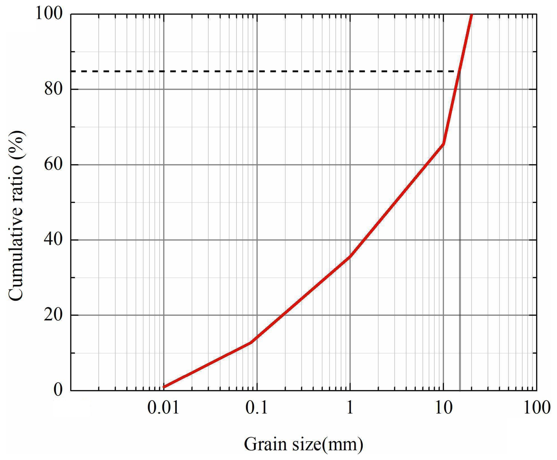
Figure 2 Grain size distribution of the flowing material considered in this study (laboratory scale).

Table 1 Flow material mixture composition.

This material was mixed until it was released to remain unconsolidated. The flume was cleaned after and before each test by water flushing to eliminate any solid material (sediment residual).

2.3 Barrier

The barrier model used in the experiments was designed to resemble real structures while considering similitude requirements. By contrast with previous research on small-scale experiments where a debris flows was intercepted by a flexible barrier, the barrier characteristics were determined to achieve mechanical similitude with the real scale. This was recently described by the authors in Lambert et al. (2024), in view of addressing the use of flexible barriers for trapping woody debris during floods (Piton et al., 2023; Lambert et al., 2023).

The model corresponds to a real barrier 13 m in length and 4 m in height, comprising a net supported and laterally fringed with 24 mm in diameter steel cables, 150 GPa in tensile modulus. The metallic net consists of the repetition of a water-drop mesh. This type of net was initially developed to be the interception structure in rockfall protection barriers (Bertrand et al., 2012) before being considered for applications in torrents (Lambert et al., 2023, 2024). By contrast with real barriers, the model doesn't integrate any energy dissipators, which have a significant influence on the horizontal cables loading and on the barrier deflection (Albaba et al., 2017; Ng et al., 2016). To the best of our knowledge, the present study is the very first that addresses the trapping of debris flows considering a down-scaled flexible barrier (though without energy dissipators).

The net model was 100 mm × 330 mm in dimensions, with a diamond-shape unit mesh, 9.4 mm × 20.6 mm in dimensions (Fig. 3). The mesh opening smallest dimension is thus much smaller than quantile 90 % of the grain size distribution shown in Fig. 2 which guaranteed the trapping of the debris flow (Wendeler and Volkwein, 2015). Indeed, although a little bit of interstitial fluid passed through the flexible barrier during impact, the high granular content of the flows resulted in an almost instantaneous clogging of the structure (see the Supplement Videos).

The flexible barrier was 3D printed from PETG (polyethylene terephthalate glycolized – see Lambert et al. (2023) for its description and its design). The net was supported by 3 lines of horizontal cables 330 mm in length, located at the bottom, mid-height and top of the net, and laterally fringed by 2 vertical cables 100 mm in length (wing cables) as illustrated in Fig. 4a. Each line of horizontal cable consisted of 1 or 2 parallel 3D printed cables. In a few test cases, it consisted in a metallic cable 0.3 or 0.5 mm in diameter. On the contrary, each wing cable consisted in one 3D printed cable only. The 3D printed cables were made from a stereolithography resin (type JS-UV-2018-01). Pairs of 3D printed cables and metallic cables were employed in lieu of single 3D printed cables in horizontal cable lines to prevent from failure. Indeed, tests involving a high released mass or a high flume inclination often resulted in cable failure when each horizontal line consisted of only one 3D printed cable. The influence of the differences in mechanical characteristics of the horizontal cable lines will be briefly addressed when dealing with the barrier loading, in a forward-looking initiative. The mechanical connection between the net and the horizontal and wing cables was insured weaving the later in the former. The extremities of the vertical cables were connected to the extremities of the upper and lower horizontal cable lines (Fig. 4a). The flexible barrier model was installed at the flume outlet, normal to the flowing direction.

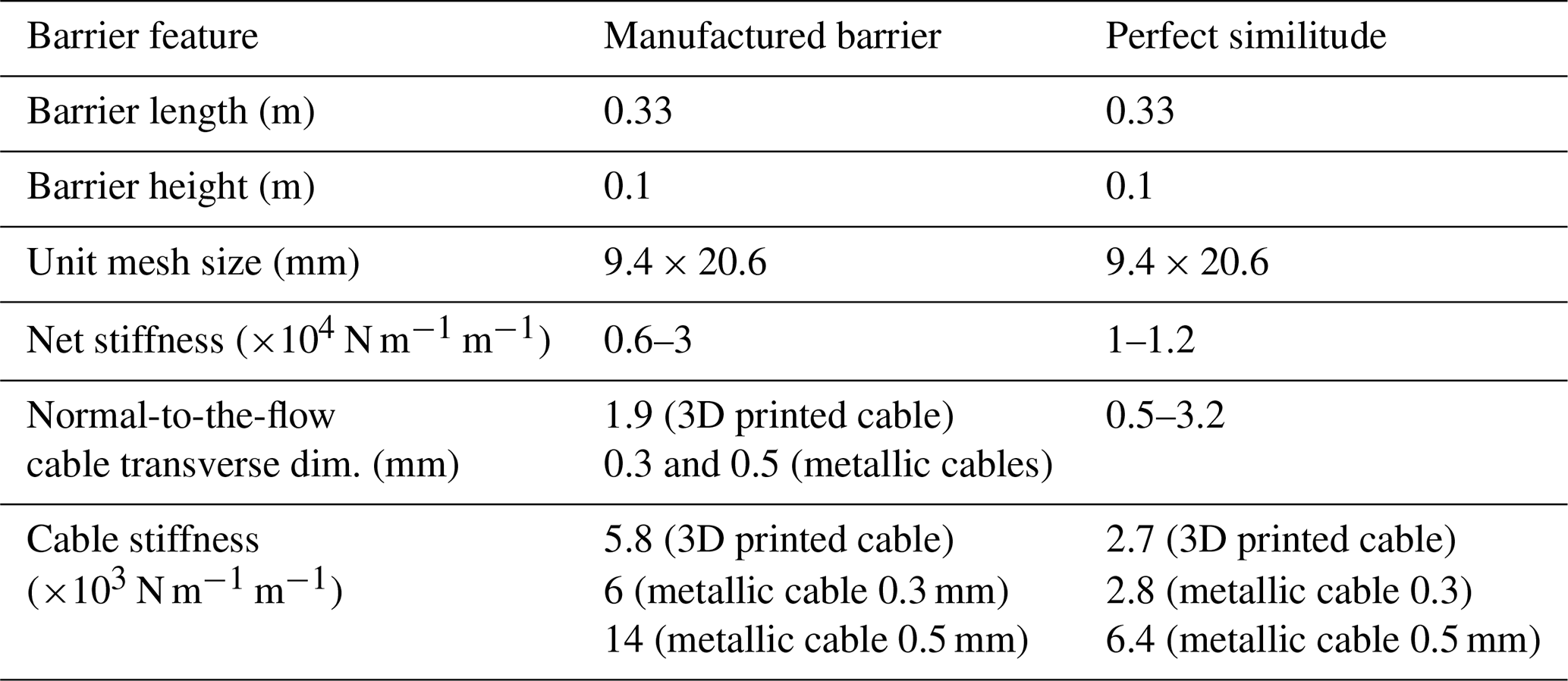
The main characteristics of the barrier models are presented in Table 2. The last column gives the ratio between the model parameter value and the value of this parameter meeting similitude requirements. Due to some manufacturing constraints, perfect similitude is not achieved for some cable characteristics (i.e. cases where the ratio ≠1). For example, the 3D printed cable stiffness is slightly too large. In spite of this, it is believed that the barrier model response is representative of that of the real scale prototype. As for metallic cables, similitude was not a requirement but it is noteworthy that the stiffness of the 0.3 mm in diameter steel cable is close to that of the 3D printed cable.

Figure 3 Flexible barrier model: the 330 × 100 mm net (a) and cables (b).

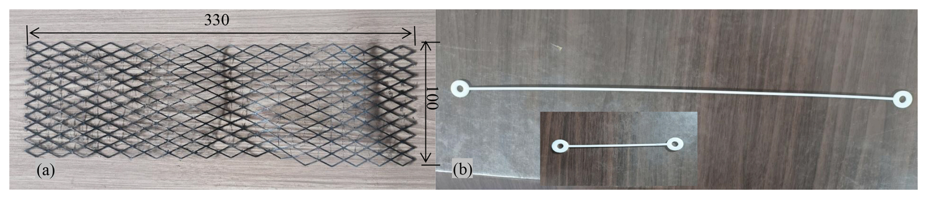
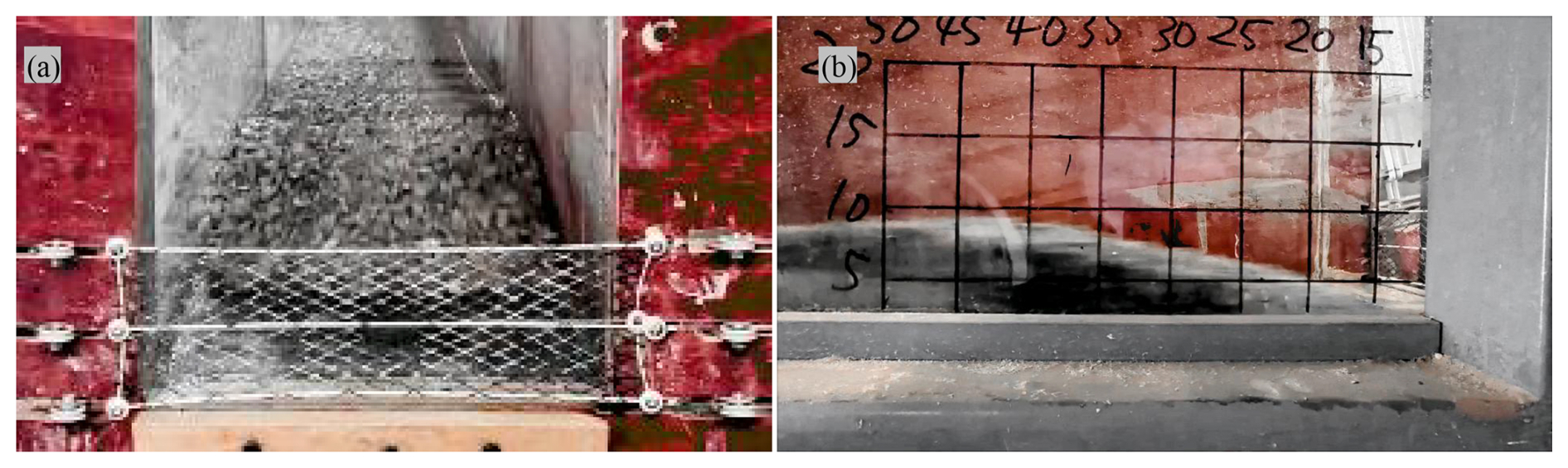
Figure 4 Picture from (a) the front and of (b) the side of the flowing material before it reached the barrier (Test 13-100-3D1).

Table 2 Characteristics of the flexible barrier models.

2.4 Measurements

Equipment used during the experiments aimed at measuring the flow velocity and depth upstream the barrier, the barrier elongation along its length and the force in the barrier horizontal cables.

Ultrasonic sensors (US) were installed 0.5 m above the flume bottom with their main axis normal to the flume bottom. Sensors 1 and 2 were respectively installed 0.6 and 0.1 m upstream from the flume outlet and barrier position. The collected data were used for determining the front velocity and the depth (or height) of material above the flume base during the test (see Sect. 2.5).

Two cameras were installed on the side and in front of the channel to record the profile and frontal views of the flow-structure interaction. The side views show the scene from a 10 cm distance from the barrier approx. These images were used to analyse the flow evolution during its interaction with the barrier (see Sect. 3.2.1) and also for providing an estimate of the maximum depth.

The three horizontal cables were equipped with force and elongation sensors. More precisely, the eyelet at one extremity of each cable was connected to a force sensor with a 1000 N capacity. Elongation of the barrier was recorded using displacement sensors which wire ran along the barrier cable to which it was secured, in a similar manner as in Piton et al. (2023) and in Lambert et al. (2023). The displacement sensor accuracy was as small as $\mathrm{1}\times {\mathrm{10}}^{-\mathrm{4}}$ mm. The absence of energy dissipators on the cables allows to measure only the cable and barrier responses.

Dataloggers with a sampling rate of 100 Hz recorded the ultrasonic and draw wire sensors measurements. Synchronization between time series were performed based on time of impact defined based the elongation measurements.

2.5 Data post processing

Data collected during the tests were post-processed to derive the flow velocity and loading on the barrier. The approaching flow depth depth, h_f was determined from data collected from US1. Data from US2 aimed at sensing the surge incoming right before impacting the barrier. The approaching debris flow front velocity, U, was determined from the time lag between the two ultrasonic sensors which were 0.5 m apart (Vagnon and Segalini, 2016; Hürlimann et al., 2019; Ng et al., 2019). Given that this type of sensor measures the distance within a cone, contrary to laser sensors for example (Wang et al., 2022), the collected data were post-treated with the Pearson correlation method to obtain the time lag. The principle is basically illustrated in Fig. 5. To cross control that the time lag was correctly assessed, the downstream signal is also shifted in the figure by the computed time lag. If the continuous increase part of US1 correctly align with the shifted part of US2, it means that the time lag is coherent. In the rare cases where the automated computation of the front velocity was not consistent (misaligned dotted pink line with the continuous blue line), a verification and estimation based on the signal and videos was performed.

The force sensors were mainly used to determine the force at rest, after the material has stopped flowing. Indeed, obtaining a precise measurement of the peak force was not possible due to some technical limitations with the system (slight smoothing of the force by the sensor). A few additional tests with another sensor performed after the whole series revealed that the uncertainty regarding the peak force value obtained from our experiments was in the range 10 %–20 %, sometimes possibly more. As a consequence, we decided not to focus on the peak force measurements but rather to analyse the force values at rest as it was not biased by the smoothing. The measures collected from these sensors after all the material was at rest will be used in Sect. 3.3.2 for estimating the total force transferred to the barrier anchors (force within the barrier) and in Sect. 3.3.3 for estimating the total load exerted on the barrier, according to Appendix A.

Video images from the front were used to assess cases that resulted in overflow and also allowed identifying barrier failure cases. Video images from the side were used for assessing the flow profile evolution during the test. These video images were also used to obtain the maximum flow depth observed during the whole test, h_max, and the deposit depth at rest measured 0.1 m upstream the barrier, h_d. This distance was the distance between the barrier and the right boundary of the 50 × 50 mm grid on the transparent lateral wall (see Fig. 4b). The use of the side video images in this purpose was motivated by the fact that measurements with US2 revealed not reliable in the frequent cases where the deposit surface was not parallel to the flume bottom.

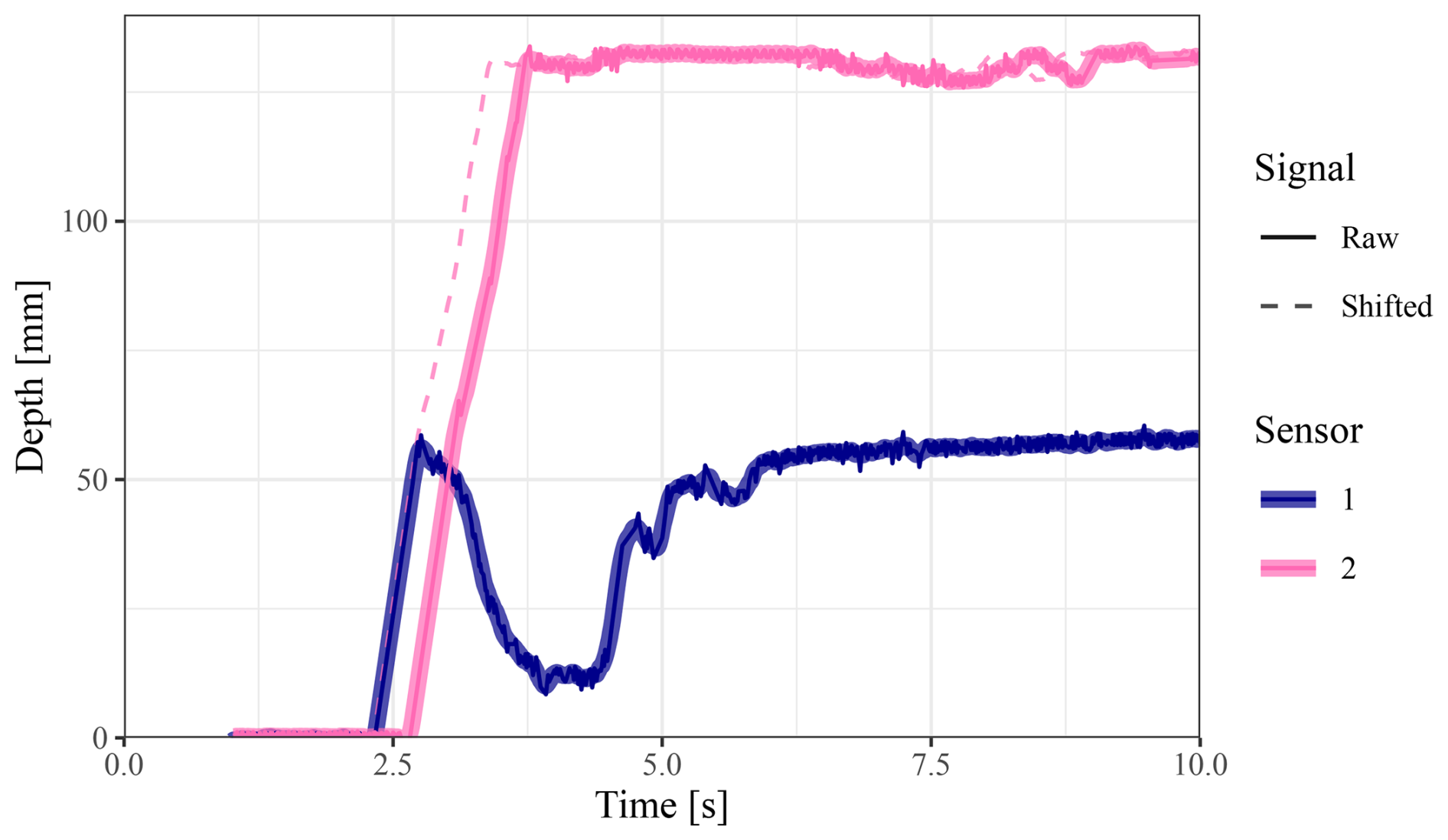
Figure 5 Flow depth time series (raw signal in continuous line) and shifted downstream measurement (dotted line) to cross check that the time lag deduced from the correlation analysis correctly align the flow level of the surge front.

2.6 Experimental plan

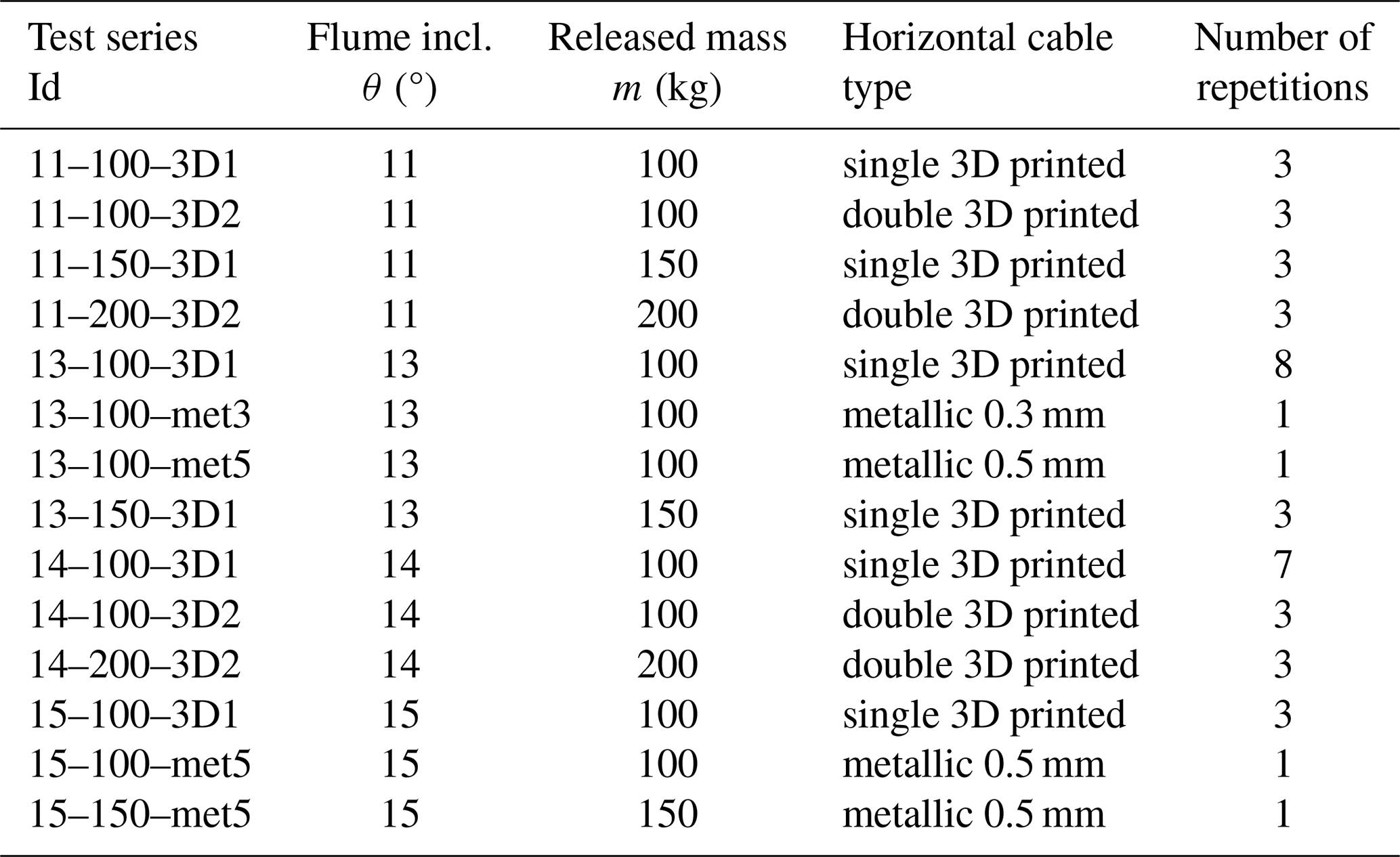
This study focuses on the interaction between a single surge debris flow and a flexible barrier. In view of accounting for different flow dynamics, the total mass of the released mixture, m, and flume inclination, θ, were varied. Some combinations of m and θ resulted in cable failure while the material was still flowing. This notably occurred with θ⩾14° and/or m=200 kg. The corresponding data were discarded from the study. In order to conduct tests at large m and θ values, the flexible barrier design was modified adding one supporting horizontal cable at each position as is done in practice when anchor strength is insufficient. The tests considered in this study are listed in Table 3. Each test is named according to a code, e.g. 11-100-3D1 listing the inclination (11, 13, 14 or 15 in °), the mass released (100, 150 or 200 in kg), the type of cable (“3D” for 3D printed or “met” for metallic) and whether or not the cables were doubled (“3D1” are single 3D printed cables while “3D2” are doubled 3D printed cables).

For series where 3D printed cables were employed, at least three tests repetitions were conducted. Only one test per series was conducted for series with metallic cables, as these structures were considered in a forward-looking initiative, for comparison purpose and also to address higher mass and inclination values. A higher number of repetitions was considered for test series 13-100-3D1 and 14-100-3D1. In the first case, this was due to minor differences in barrier design concerning the lateral cables. In the second case, three tests resulted in a late and partial barrier failure and, even though this induced very marginal effect on the deposit volume and shape, additional tests were conducted. These differences were accounted for when analysing the results in view of considering consistent data sets with respect to the addressed topic (e.g. results from tests during which late cable rupture was observed were considered when dealing with the incoming flow evolution but not for addressing the barrier response).

Table 3 Experimental plan.

3 Results

3.1 Approaching flow

Figure 4 illustrates the behaviour of the flowing material before reaching the barrier from front and side views. Very similar trends were observed in other test conditions. First, the front consists of a rather homogeneous mixture of large and fine particles (Fig. 4a). Second, the flow front is clear and rather steep rising from a dry bed to its maximum in about 25–30 cm (Fig. 4b). In all cases, the flow depth remained rather constant over a rather long distance after this maximum value was reached.

The mean values out of all experiments for the flow front velocity and depth h_f depth were approximately 1 m s⁻¹ and 7.5 mm, respectively. These characteristics revealed significantly variable from one test condition to another, depending on the released mass and flume inclination (Fig. 6). In particular, the larger the released mass, the higher the flow depth (Fig. 6a). By contrast, no clear influence of the flume inclination on the flow depth can be observed on the considered range. Meanwhile, as expected, a higher inclination results in a higher velocity, for all released mass (Fig. 6b). However, there is no clear trend for the influence of the mass on the velocity. In brief, the released mass had an influence on the flow depth while the inclination had an influence on the flow velocity.

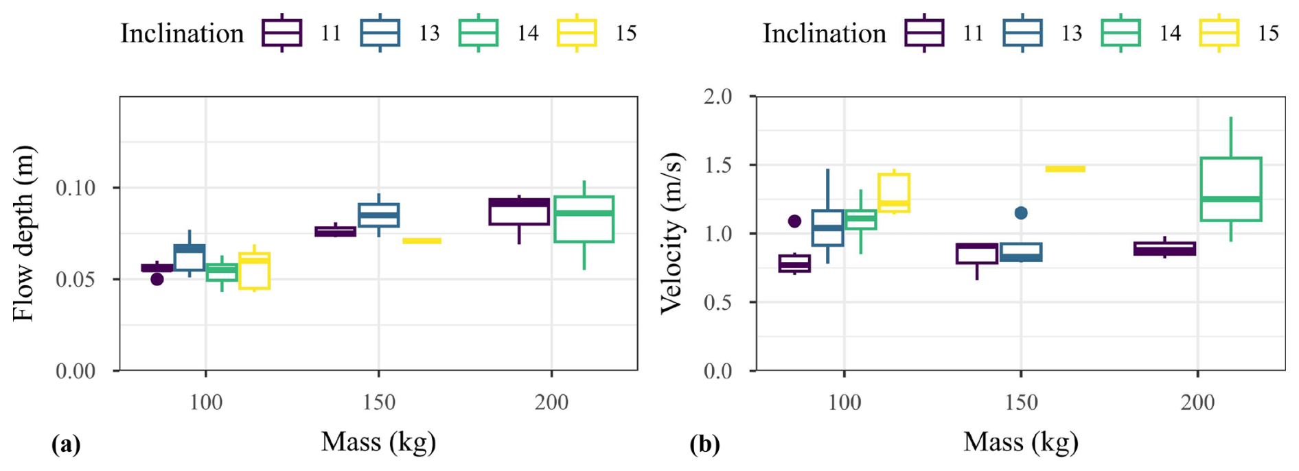
Figure 6 Depth (a) and velocity (b) of the flow before reaching the barrier varied with released mass.

In the absence of measurements of dynamic viscosity within debris flow, Reynolds number is not warranted as the scaling index in this study. Froude number, Fr, is the dominant parameter to verify the flow conditions and scaling basics (Fig. 7). Fr was computed from the flow velocity and depth measurements and revealed to range from 0.9 to 2.0. The flow regime was thus subcritical to supercritical (Faug, 2021). Fr globally showed an increase trend with the increase in inclination. By contrast, no influence of the released mass on Fr was evidenced.

Figure 7 Fr vs inclination (a) and released mass (b). All tests conditions.

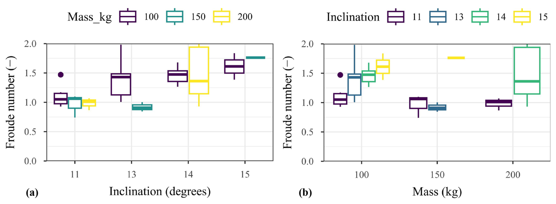
The box plots in Figs. 6 and 7 reveal a variability in flow characteristics among tests conducted with a same mass and same inclination. For instance, releasing a 100 kg mass in the flume inclined by 13°, Fr ranged from 1 to 2, approx. These observations reveal that having a well defined composition for such a mixture is not sufficient for obtaining the same flow characteristics for a given flume inclination θ and released mass m. We believe that the observed variability is partly attributed to the difficulty, for such a mass of that high solid fraction mixture made of coarse and angular grains, in ensuring the very same state at flow initiation and also to some associated segregation effects. To our experience, this effect is more limited in a steeper flume but it would result in excessively fast flows as yet discussed. This variability in Fr which is also observed in the field within a given stream (see e.g. McArdell et al., 2023; Lapillonne et al., 2023; Nagl et al., 2024), clearly justifies conducting test repetitions. In addition, this variability suggests that comparison between test results should rather consider the effective incoming flow characteristics (i.e. approach flow depth velocity and Fr) rather than the test conditions (flume inclination or mass).

3.2 Flow evolution after contact with the barrier

3.2.1 Interaction modes

The influence of the barrier on the flow evolution is generally described according to two interaction modes, referred to as “pile-up” and “run-up”, which occurrence depends on the flow characteristics (frictional or viscous) (Armanini and Scotton, 1993; Sun and Law, 2015; Faug, 2021; Ashwood and Hungr, 2016; Kong et al., 2021), which in turn could affect the derivation of the impact force. In essence, the run-up interaction refers to the flow forming an upward jet along the barrier. By contrast, the pile-up interaction (which is also referred to as momentum jump mode e.g. in Albaba et al., 2018; Song et al., 2023), is associated with the formation of a reflected wave (or granular jump), which is attributed by some academics to a progressive accumulation of material over the dead zone formed close to the barrier. This contrasts with observations made in this study increasing the mass and flume inclination which revealed a gradual change in interaction mode (in terms of accumulation, deposition and overflow) from a gentle one where all the material was arrested quietly and almost instantly to a dynamic one with overflowing.

The effect of the barrier on the flow was analysed based on the side and front videos (see some of them in the Video Supplement). The observed trends are detailed in the sequel. These global trends appeared rather independent on the cable types and number. Consequently, the videos analysis focused on the factors in relation with the mass released and flow characteristics which best explained these trends notably through a mass integration of the energy specific head while assuming a uniform flow depth, equalling h_f, – a reasonable first order approximation – which leads to:

$$\begin{array}{}\text{(2)}& E=mg{h}_{\mathrm{f}}(\mathrm{1}+F{r}^{\mathrm{2}}/\mathrm{2})\end{array}$$

Globally, four different modes could be identified, all described in the following paragraphs. The first was the quasi-solid body behaviour (mode I). The second was the granular buckling dominated mode, without overflowing and with limited evidence of granular jump (mode II). Mode III was related to cases with a pronounced granular jump but without overflow. Mode IV concerned all cases where the material accumulation upstream the barrier was followed by overflowing.

Mode I consisted in a gentle interaction where the flowing material almost behaved as a solid body at its interception. Once a volume of material was arrested, it was exposed to compaction by the incoming material, basically resulting in a decrease in length of the arrested material (along the longitudinal axis of the flume) and in its expansion in the direction perpendicular to the flume bottom, most probably through grain local rearrangement and compaction (Fig. 8a). This process started in the barrier vicinity and concerned almost instantaneously all the released volume, without any overflow of previously arrested material by subsequent incoming material. The vertical expansion was uniform along the flume length. It resulted in a deposit surface almost parallel to the flume bottom, with a deposit depth h_d slightly higher than the approaching flow depth (with an average ratio of 1.2). This interaction mode was observed for a limited number of cases where the flow energy was about 100 J and Fr≈1.

The increase in flow kinematics (velocity and flow energy) resulted in mode II characterised by a higher expansion of the arrested material combined with a free surface shape change with time. In fact, the depth increase started at the barrier and propagated upstream as a low to very low amplitude reflected wave (i.e. resembling a granular jump) (Fig. 8b). By contrast with mode I, it seemed that the compression generated by the incoming flow resulted in instability in the accumulated material (mechanism similar to chain forces buckling in granular materials) which explains the higher deformation of the accumulated material. No material flowing over the yet-arrested material at the barrier bottom could be visually observed. As a result of the significant vertical expansion, the depth of the deposit, h_d, exceeded the barrier initial height, h_B, by up to 50 %. During some tests, some particles from the surface of the accumulated material, in the barrier vicinity, were destabilised and felt beyond the barrier. The deposit had a variable depth along the flume length and exhibited a concave shape with a depth in a 10–15 cm typical range. This mode was the most frequently observed and concerned all flume inclinations, velocities and Froude number values, and flow energies over a wide range and up to 180 J.

Although their flow energy can be similar (i.e. <170 J), more pronounced granular jumps were observed in mode III having flows with a Fr>1.2, which appear mostly at flume inclinations of at least 14°, without any clear relation with other factors (Fig. 8c). This mode is assimilated to the momentum jump mode (Albaba et al., 2018) but the way the granular jump formed (e.g. by incoming material piling up above the arrested material) could not be determined visually. In these cases, the deposit depth in the barrier vicinity was much more than twice the incoming flow depth.

Massive overflow was observed in mode IV with E in a 200–350 J typical range (Fig. 8d). In fact, the occurrence of overflow was more clearly related to the released mass, as all cases with a mass of 200 kg resulted in barrier overflow. One case where the mass equalled 150 kg resulted in overflow. Overflow occurred after a significant volume of material accumulated upstream the barrier, with a well-marked granular jump in some cases (meaning step-like). The depth reached a maximum value, h_max, typically twice the barrier height, h_B. By contrast with interaction modes I–III, the depth significantly decreased with time as the material previously deposited above the level of the top of the barrier was flushed downstream by the subsequent flowing material. The overflow lasted about 10 s, which contrast with modes I–III cases during which all the material visible from the side videos was stopped in <2 s. In case of overflowing, the deposit depth at rest, h_d, was slightly higher than the barrier initial height (typically 0.12 m) and the surface of the deposit was nearly parallel to the flume bottom. For two tests only, the deposit surface was convex with a deposit depth h_d up to 0.16 m.

In the specific case illustrated in Fig. 8e, massive overflow was observed after the flow ran-up along the barrier. This was the only case where run-up with an upward jet was observed. Compared with cases in similar tests conditions, this flow was characterized by high velocity, low depth, high Fr (1.8), and energy >400 J. This was related to an apparent lower solid fraction of the flow front which resulted from some segregation effects at flow initiation, as mentioned before. For these reasons, this case was considered marginal and thus not representative of the system response in the test conditions ranges.

The analysis of the side videos from the moment the flow front touched the barrier to the situation at rest thus reveals that the interaction between the flow and the barrier was variable depending on the test conditions, in terms of the flow evolution, material accumulation and deposition and barrier overflowing. It also revealed it could hardly be described in a binary way as often done in the literature, where pile-up and run-up are proposed as the two processes by which an obstacle modifies the flow kinematics. On the contrary, a progressive shift between four typical modes was observed. These differences with descriptions from the literature are thought to be related to the differences in flowing material characteristics (wide range of grain size from clay to boulders) and in flow conditions, and in particular the careful exploration of near-critical debris flows with a rather narrow Froude number range.

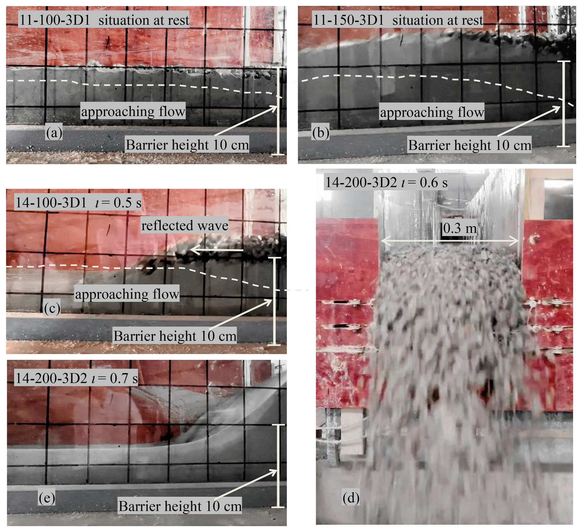
Figure 8 Illustration of the different modes observed: (a) quasi-solid body behaviour, mode I (b) granular buckling dominated, mode II, (c) pronounced granular jump, mode III and (d) massive overflow, mode IV. Marginal case of quasi-vertical jet (e). The time reference (t=0) corresponds to the moment when the flow front touched the barrier. The dotted line shows the surface of the flow at t=0. The scale is given by the 50 × 50 mm grid which starts 0.1 m from the barrier.

3.2.2 Depth variation and energy dissipation

The increase in depth resulting from the flow interaction with the barrier was addressed based on the ratio β, between the maximum flow depth recorded during the test, h_max, and the incoming flow depth, h_f.

This ratio was determined for comparison purpose between the different tests, based on the side video images. This ratio was considered by some authors and two analytical expressions relating β with Fr have been proposed. The first expression was proposed assuming energy conservation in the case of slow flows (Faug, 2021):

$$\begin{array}{}\text{(3)}& {\mathit{\beta }}_e=\mathrm{1}+{\displaystyle \frac{F{r}^{\mathrm{2}}}{\mathrm{2}}}\end{array}$$

where the debris flow is simplified as an incompressible and homogeneous fluid (Scheidl et al., 2023). The second expression was established based on the momentum jump theory which considers an abrupt change in the flow depth (with Fr<10) during the impact (Armanini, 2009):

$$\begin{array}{}\text{(4)}& {\mathit{\beta }}_m={\left(\mathrm{1}+\mathrm{1.5}F{r}^{\mathrm{1.2}}\right)}^{\mathrm{5}/\mathrm{6}}\end{array}$$

Both equations also rely on the hypothesis that all the material is stopped by the obstacle which is consistent with our experiments except for the mode IV results.

As shown in Fig. 9, experimental β values ranged from 1.2 to more than 3.3. The observed scattering is mainly attributed to the variability in flow characteristics. In spite of this scattering, some general trends can be observed. The positive correlation of β with Fr is basically explained by the fact that increasing the flow velocity induces an increase in accumulation depth during the interaction of the flow with the barrier. This figure also reveals a dependence on the interaction modes shown in Fig. 8. Interaction modes I and II globally result in lower β values, even at relatively high Froude numbers. Measures related to mode II cases are significantly scattered. Higher values of β over the whole range of Froude number are associated with mode III and, to a slightly lesser extent, with mode IV. This suggests that higher depths were reached during mode III cases, because there was no overflow.

This figure also shows a comparison of the experimental values with theoretical predictions based on Eqs. (3) and (4). This comparison was addressed quantitatively by considering the mean of the relative difference between the measured value and the predicted value for the same Froude number. β values for cases where interaction modes I and II were observed reveal globally closer from predictions based on Eq. (3). The mean differences with the prediction is 14 % while comparison with predictions based on Eq. (4) reveals differences of −20 % and −17 % for modes I and II, respectively. On the contrary, β values for cases where modes III and IV were observed are globally closer from predictions based on Eq. (4): the mean relative differences between the experimental value of β and the prediction were −5 % and −1 % for modes III and IV, respectively, compared to mean differences of 21 % and 40 % considering predictions based on Eq. (3). The fact that β values measured during tests classified as modes I and II were better predicted with Eq. (3) suggest that these modes were associated with lower energy dissipation, in particular by comparison with cases where modes III and IV were observed. The lower energy dissipation for the first two modes is attributed to lower relative displacements between particles and thus associated friction dissipation during tests where these modes were observed.

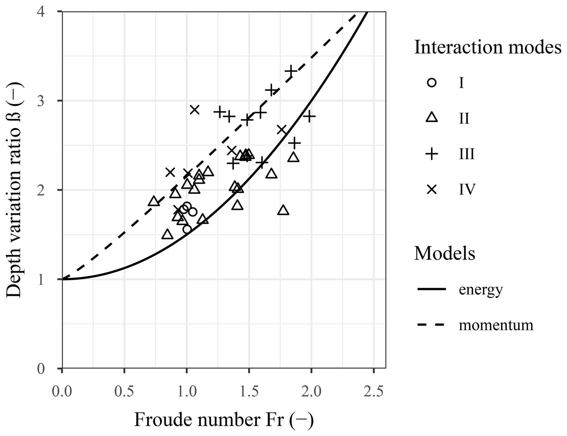
Figure 9 Flow depth variation rate as a function of the Froude number. The curves are calculated by the energy and the momentum conservation hypothesis. I, II, III, and IV refer to the interaction modes illustrated in Fig. 8.

Depth measurements after the flow had stopped revealed that more than 90 % of the tests resulted in a final deposit depth surpassing the initial barrier height. The ratio $h_{\mathrm{d}}/h_{\mathrm{B}}$ between the deposit depth, h_d, and the barrier initial height, h_B, ranged approximately from 0.9 to 1.6. The fact that this ratio was higher than one is attributed to the coarse nature of the flowing material, with a large ratio of large and angular particles and to the influence of the deposit on the flow propagation. With the progressive debris deposition, starting from the barrier, the propagation of subsequent flowing material towards the barrier is hindered due to friction with the deposited material and to a lower angle for the flow to propagate. Consequently, the flowing material deposits in such a way that the deposit apex moves away from the barrier, resulting in a deposit surface with a concave shape. The slope of the deposit surface close to the barrier is thus higher than the flume inclination, which is attributed to the granular nature of the material and to the angularity of the larger particles it contains.

3.3 Barrier response

The barrier response to the loading exerted by the debris flows is first addressed focusing on its deformation. Then, it is addressed in terms of barrier loading, focusing on the situation at rest, in the aim of evaluating the relevance of existing analytical models as for the static component of the loading on the barrier.

3.3.1 Barrier deformation

When the flow reaches the barrier, this latter experiences increasing deformation over a 1s duration typically, as illustrated in Fig. 10. This figure also reveals the difference in amplitude and variation with time of the elongation experienced by each cable. The bottom and middle cables are the first to experience elongation, in accordance with the filling dynamics. In this case, the larger elongation was observed at barrier mid-height. This may be attributed to the fact that this cable holds the net above and below it, while the bottom and top cables only hold the net above or below, respectively. The resulting difference in barrier deflection along the vertical axis is illustrated in Fig. 10b. The deformation pattern along the vertical axis was observed to significantly vary from one test condition to another. In particular, the relative deformation of the top cable with respect to the two others was much more in mode IV cases compared to that in other cases (Fig. 11). This specific feature in the deformation pattern suggests a difference in loading distribution from bottom to top which is considered as a reminiscence of the occurrence of the overflow. This was previously suggested by Wang et al. (2022). In addition, cables globally experience a much larger elongation after tests where mode IV was observed.

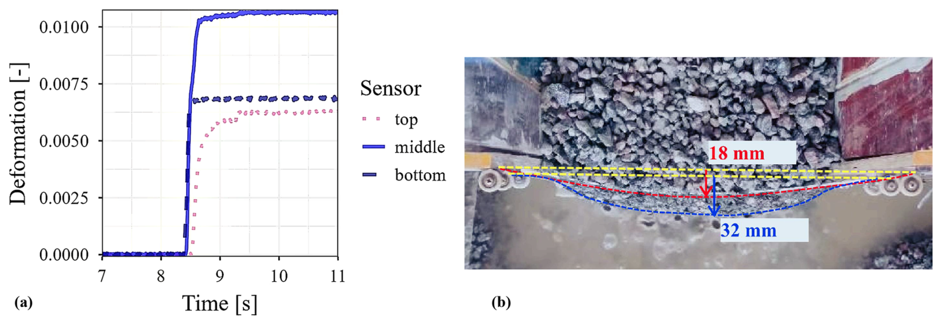
Figure 10 Typical barrier deformation: (a) evolution with time of the deformation of each cable and (b) picture from the top showing the barrier deflection (red line shows the top cable and blue line shows the middle cable).

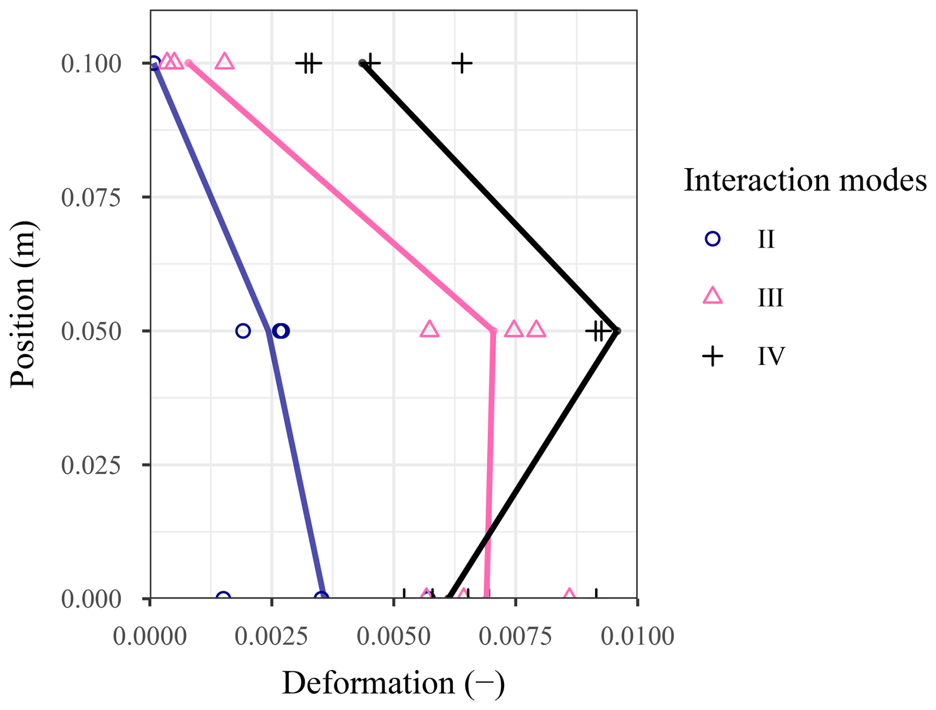
Figure 11 Cable vertical position versus relative deformation after tests involving cable type 3D2. Dots figure individual tests while the continuous lines figure mean values distinguishing the different modes.

3.3.2 Load within the barrier at rest

The load within the barrier is addressed based on the force measured by the three force sensors, which gives an indication of the amplitude of the force transiting through the barrier towards the barrier anchors. In this aim, the sum of the three forces measured when the system was at rest, F_w, is plotted in Fig. 12 showing that the force within the barrier increases with both the inclination and the released mass. In addition, a high dependency of F_w on one parameter is observed when the value of the other is small. For example, the flume inclination has almost no influence on F_w when the released mass is 200 kg, while it is very large when 100 kg of material is released.

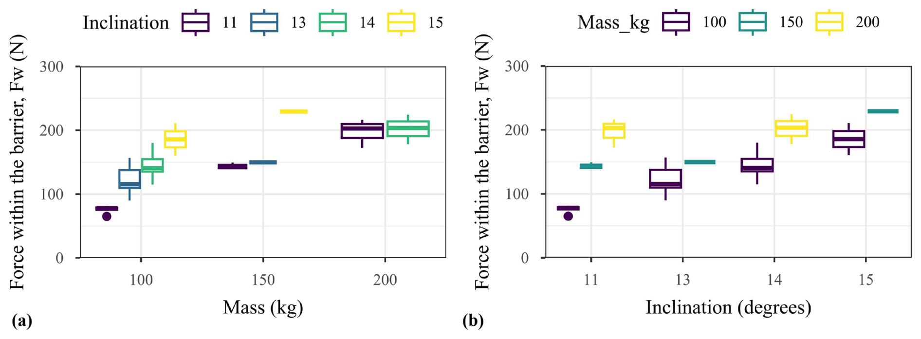
Figure 12 Force within barrier at rest, F_w, as a function of (a) the released mass and (b) the flume inclination.

Similarly as for a retaining wall, the loading applied by the retained material on the barrier and consequently the force within the barrier, F_w, are expected to be related to the deposit depth, h_d. This is globally confirmed in Fig. 13a. The influence of this parameter appears larger than that of the flume inclination (Fig. 13b). However, a rather large variability in F_w is observed for a given depth or a given inclination. This variability is first attributed to the interaction mode. F_w values were always higher for mode IV cases, which are associated with barrier overflow.

Restricting the analysis to modes I–III cases reveals that the variability in F_w is also related to the characteristics of the horizontal lines of cables. F_w was lower when each horizontal line consisted of one 3D printed cable. Replacing these cables with pairs of 3D printed cables, 0.3 mm and 0.5 mm in diameter metallic cables resulted in increasing values of F_w, for a given depth. For example, the average value of F_w for a 0.12 mm deposit depth increased by about 70 % when pairs of 3D printed cables were used in place of single 3D printed cables. In fact, stiffer cables restrict the barrier deflection and associated energy dissipation by granular friction of the depositing material and, consequently, result in higher forces in the supporting cables. This observation confirms the importance of accounting for similitude of flowing material and of the flexible barriers in designing barriers to be used in small-scale experiments (Lambert et al., 2023).

The number of tests performed did not allow us deriving analytical expressions for reflecting these trends while accounting for all the varied parameters. However, these results rather clearly indicate that the static loading in the barrier, and thus the loading it experienced, does not depend only on its depth measured at rest upstream the barrier.

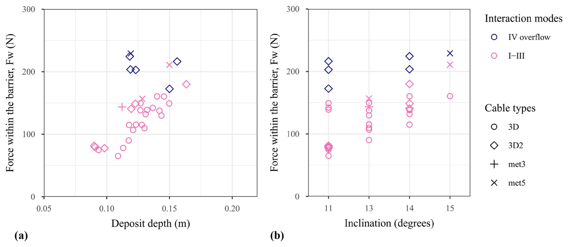
Figure 13 Force within the barrier at rest, F_w, as a function of the deposit depth (a) and as a function of the flume inclination (b).

3.3.3 Loading on the barrier

While the force within the barrier, F_w, is based on measurements transverse to the flow direction, it is possible to estimate the load exerted by the debris flows on the barrier, F_b, from the elongation and force measured at each cable extremity. The different available analytical models used in this purpose rely on various assumptions, in particular regarding the distribution and orientation of the loading on the barrier and the barrier deformation along its longitudinal axis (Brighenti et al., 2013; Ng et al., 2016; Song et al., 2018, 2019; Tan et al., 2019; Kong et al., 2022). In this study, the load distribution was considered uniform and the shape of the deformed barrier was considered to be circular or parabolic. Appendix A provides the analytical expressions considered for estimating the total force applied on each cable from the force and elongation measurements. F_b was computed as the sum of the total force acting on the three cables. Similarly as for F_w, F_b was computed from the measurements at rest only and do not concern the peak value which is reached when there is still material flowing.

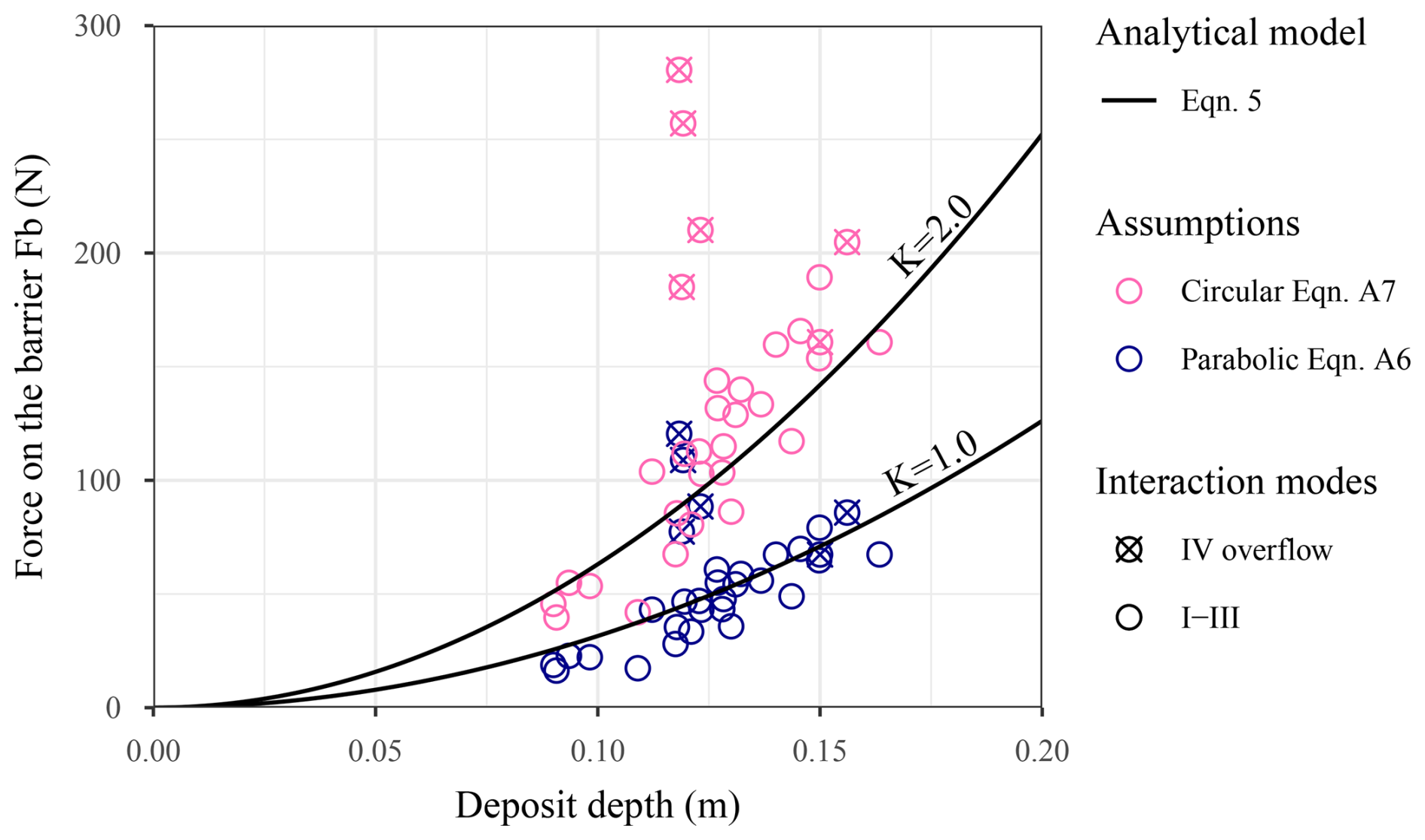
Figure 14 Force applied on the barrier at rest, F_b, as a function of the deposit depth. The dots in the pink and dark blue points with crosses refer to overflow cases (i.e. interaction mode IV).

The force acting on the barrier when at rest was also estimated based on a classical analytical expression from the literature dealing with the design of structures exposed to debris flows. This static force, F_s, was computed as follows:

$$\begin{array}{}\text{(5)}& F_{\mathrm{s}}={\displaystyle \frac{\mathrm{1}}{\mathrm{2}}}K\mathit{\rho }g{h}^{*\mathrm{2}}B\end{array}$$

where K is the lateral pressure coefficient, which is generally set to 1.0 assimilating the loading to the hydrostatic case, as in Berger et al. (2021). ρ is the deposited material unit mass, which was set to 2200 kg m⁻³ from the measurement on the initial mixture. B is the barrier length. h^* is the depth of material upstream the barrier. In design practices, h^* is the depth of material at rest close to the barrier and never exceeds the barrier initial height. This depth was not measured during the experiments. In lieu, h^* was considered equal to the deposit depth, h_d, which was measured 0.1 m from the barrier, keeping in mind that this value was generally higher than the depth close to the barrier and often revealed higher than the barrier initial height by a ratio of up to 1.6.

The first general observation derived from Fig. 14 is that the circular shape assumption for the barrier deformation results in a total force F_b much higher than that computed considering the parabolic assumption, with a ratio up to three for some tests. This observation is in line with some previously published research stating that analytical solutions might introduce significant errors in estimating the total load on flexible barriers (Kong et al., 2022). It justified evaluating the validity of each shape assumption. In this purpose, the barrier deflection predicted by each model was compared to that measured based on images from the top as shown in Fig. 10b. For this case, the parabolic assumption (Eq. A2 in Appendix A) resulted in deflection values of top and middle cables of 14 and 20 mm, respectively. Values of 36 and 52 mm were respectively obtained considering the circular shape assumption (Eq. A8 in Appendix A). Comparison with the measured values (18 and 32 mm, respectively) reveals that the parabolic assumption is more appropriate. For this reason, only results obtained based on the parabolic assumption will be considered in the following. This conclusion in terms of the barrier deformation hypothesis is a key result from a design perspective as it concerns the loading experienced by the barrier and thus its cost. It is trustworthy and useful in operational contexts as it was reached considering realistic flowing material, flow conditions and barrier, while accounting for similitude with the real scale, by contrast with most previously published studies.

The second general observation is that the value of F_b for the same depth of deposit varies from one test to another, which highlights that the deposit depth is not the only parameter controlling the barrier loading at rest. More importantly, the force in overflow cases (crossed symbols) is globally much higher than that in the cases where all the material is retained with average and maximum ratio between extreme values of about two and four, respectively.

The third general observation is that, without overflow, all points determined based on the parabolic assumption globally align with the prediction based on the hydrostatic loading model, i.e based on the analytical model expressed in Eq. (5) while considering a pressure coefficient K=1.0. This agreement was obtained considering the deposit depth and not the barrier height. Considering the barrier height would lead to a shift to the left of most of the points in Fig. 14 to an abscissa of 0.1 m, leading to the situation where there would be no more agreement with predictions based on Eq. (5). Meanwhile and in spite of a certain scattering, F_b values associated with overflow cases are closer from predictions considering a K value of 2.0. The two outliers observed on the figure correspond to the cases where the deposit surface was convex, with a much higher value of h_d than other overflow cases.

4 Discussion

In this research, a particular focus was placed on the deformation and loading of the flexible barrier when at rest, after it intercepted a debris flow. The motivation for this was that the static component of the force exerted by the deposited material (or dead zone) on the barrier received limited attention up to now while it may have a major contribution in the barrier loading, and in particular the case when the flow Froude number is in the range of events observed in Alpine environments. The postulate on which this approach is based is that the force exerted at rest on the barrier can be assimilated to the maximum static component of the force exerted on the barrier during an event. This situation may correspond to a given time instant during the progressive debris accumulation or to the case of a surge reaching the barrier which already caught debris material. Because in this study the ratio between the deposit depth and the barrier initial height, $h_{\mathrm{d}}/h_{\mathrm{B}}$, ranged approximately from 0.9 to 1.6, these results rather concern the second situation with a filled or almost filled barrier.

The $h_{\mathrm{d}}/h_{\mathrm{B}}$ ratio ranging up to 1.6 can also be read in another way: the surge depth varying in the 50–100 mm range (Fig. 6), the total deposit in case of filling without massive overtopping can be computed as the sum of the barrier height plus the depth of an approaching surge that would stop right before the barrier. In our test campaign, the maximum deposit height is indeed about the barrier height plus the average of the surge height between every tests. Considering the maximum surge height would be too conservative because the biggest surges are also more mobile and thus less likely to stop right at the barrier. Consequently, it is believed that this large ratio refers to this barrier height, and that it would reduce increasing by the barrier height.

It was shown that, in absence of overflow, the total force applied at rest on the barrier, F_b, could be reasonably modelled assimilating it as an hydrostatic loading for any deposit depth using Eq. (5) and considering the debris material unit mass and K=1. This K value is in agreement with that suggested by various authors as well as in design recommendations (Wendeler et al., 2019; Berger et al., 2021, among others). However, this conclusion was reached considering the depth of the deposit at rest, h_d, and not the depth of the deposit in contact with the barrier as generally done (Berger et al., 2024). According to this latter approach, all the points in Fig. 14 for which the depth is higher than the barrier height should be shifted to align parallel to the y-axis at an abscissa of 100 mm approx. In such a case, the agreement would be lost because the F_b value of points with this abscissa would vary over a large range, with a ratio as large as four between extreme values. Even though considering h_d resulted in a good agreement with the predictions based on Eq. (5), this approach is not rigorous on a mechanical point of view, because F_s refers to a triangular stress distribution decreasing to zero from barrier bottom to top. In lieu, F_s should rather be computed with $h^{*}=h_{\mathrm{B}}$ while considering an additional thrust induced by the surcharge, $\stackrel{\mathrm{‾}}{q}$, associated with the material deposited above the barrier. This additional thrust may be computed as:

$$\begin{array}{}\text{(6)}& F_{\stackrel{\mathrm{‾}}{q}}=K_{\stackrel{\mathrm{‾}}{q}}\mathit{\rho }g(h_{\mathrm{d}}-h_{\mathrm{B}})B{h}_B\end{array}$$

where $K_{\stackrel{\mathrm{‾}}{q}}$ is a pressure coefficient that can be assumed equal to K as a first approximation. This different approach results in slightly lower values for the force applied at rest on the barrier. Considering the observed range for h_d, the difference for modes I–III cases is less than 15 %. As this difference remains small, a force computed based on Eq. (5) while considering $h^{*}=h_{\mathrm{d}}$ and K=1 can be considered a good estimate for modes I–III cases.

A major finding in this research concerns the much higher barrier loading at rest in mode IV cases (with overflow) compared to that for other cases with a similar final deposit depth. The increase in barrier loading during overflow is generally considered as resulting from the combination of two components associated with the material flowing on the deposited material (Albaba et al., 2017; Berger et al., 2021; Wang et al., 2022). The first component is a stress normal to the deposit surface, or surcharge q, due to the weight of the flow on the deposit. The second is the shear stress (also referred to as drag force) that develops at the interface between the flowing material and the deposit (Ashwood and Hungr, 2016; Wendeler et al., 2019). Our experiments revealed that overflow also had an influence on the barrier loading after the event, which suggests that the granular body matrix kept the memory of the load it experienced during the event. Since debris flows very often present several surges and flexible barriers have only a limited capacity, most of them are expected to experience overflow in due time. In such cases, the barrier design should consider a static thrust by the deposit typically twice that usually considered. Indeed, Fig. 14 suggested that F_b could be conveniently captured with a K value of 2.0. However, this approach is not rigorous either because the complexity of the mechanisms involved is ignored and this model is not consistent with some observations. For example, the significantly higher elongation observed in the upper part of the barrier in overflow cases (Fig. 11) can hardly result from a triangular stress distribution as assumed with Eq. (5).

A more robust analytical approach consists in distinguishing the different force components acting on the barrier during overflow, similarly as conducted for modes I–III cases. The first component is the thrust due to the deposit in contact with the barrier which was computed using Eq. (5). The computed value of F_s was 32 N, considering K=1 and $h^{*}=h_{\mathrm{B}}$. The second component is associated with the surcharge due to the material above the level of the barrier top cable. During overflow this material consisted of both flowing material and arrested material (upper part of the dead zone). The depth of both evolved with time and could hardly be determined precisely from the side video images. However, the maximum depth measured during overflow cases, h_max, was in the 0.18–0.21 m range, meaning that the depth of material contributing to the surcharge q was in the 0.08–0.11 m range. The additional barrier loading induced by the surcharge on the deposit, $F_{\stackrel{\mathrm{‾}}{q}}$, was computed according to Eq. (6) with K_q=1. Replacing h_d−h_B with the depth of the material contributing to the surcharge (h_max−h_B) resulted in a 52–71 N range for $F_{\stackrel{\mathrm{‾}}{q}}$. The third component to account for relates to the loading induced by the drag force, F_d. An estimation based on Ng et al. (2024) resulted in F_d values in a 140–190 N range varying the depth of overflowing material in the 0.08–0.11 m range. The sum of these three terms, $F_{\mathrm{s}}+F_{\stackrel{\mathrm{‾}}{q}}+F_{\mathrm{d}}$, is thus estimated to amount 260 ±35 N. Based on these estimates, the contributions of F_s, $F_{\stackrel{\mathrm{‾}}{q}}$ and F_d to the total force applied on the barrier during overflow are approximately 10 %, 25 % and 65 %, respectively. The last two values are attributed to the very large depth (up to 0.21 m) measured during overflow compared to the barrier height. Besides, the total force is more than twice the force applied on the barrier at rest, F_b, for mode IV cases (indeed, a typical range of 75–120 N is observed in Fig. 14). This difference in force magnitude between F_b and $F_{\mathrm{s}}+F_{\stackrel{\mathrm{‾}}{q}}+F_{\mathrm{d}}$ suggests that the barrier experienced a peak load during overflow, followed by a significant decrease. These findings raise questions, as discussed below.

The latter conclusion as for the significant decrease with time of the barrier loading (in a ratio of 2) is in contradiction with the observation that, similarly as what is shown in Fig. 10, the barrier cables experienced very negligible decrease in deformation after reaching their maximum value. This suggests that there was no significant barrier unloading. Although not precise, measurements of the force in the cables did not suggest any significant decrease over time. This inconsistency between estimates and measurements is though to be due to the assumptions based on which the analytical models considered in this study were established. Appendix A gives the list of assumptions made for estimating the force acting on the barrier, F_b, based on the measurements made during the experiments. The barrier was assumed to deform as a parabola, while it was not always checked, in particular for mode IV cases tests. Equations (5) and (6) used for computing F_s and $F_{\stackrel{\mathrm{‾}}{q}}$, considered that the flexible barrier is a rigid and vertical wall exposed to a uniform distribution along the barrier length. These equations were used assuming K=1, which fundamentally implies that the material is considered non frictional. The surcharge, q, was supposed to be uniform along the flume axis, which differs from observations made from side videos. The analytical model for computing F_d, which was proposed for debris material and flowing conditions different from that in this study, also relies on many assumptions (Kwan, 2012; Ng et al., 2024). The relevance and consistency of all these assumptions should be further addressed, in particular with respect to low Froude number flows, with a large solid fraction material containing coarse and angular grains. In the meantime, the conclusions drawn in this study as for the maximum loading applied over time on the barrier and estimated from analytical models should be considered with caution.

5 Conclusions

This paper presents small-scale experiments of flexible barriers impacted by near-critical flows (i.e. Fr=0.9–2) of a debris material with a high solid fraction and containing a large amount of coarse and angular particles. These tests were carefully designed to model quite realistic debris flows with a mixture of gravel, sand, clay and water. The flexible barriers consisted of a cable-supported mesh and were not equipped with energy dissipators. The barrier components were manufactured with 3D printers such that their flexibility was in mechanical similitude with actual steel barriers. The impact regime and deformation of both the stopping debris-flow material and the barrier are modelled with less scale effects than in previous works using simpler mixtures (e.g. dry sand), excessively fast flows (i.e. Fr≫1) or with irrelevantly-stiff barriers (e.g. made of steel or of nylon).

Focusing on a narrower range of Fr and ensuring a relevant deformation of the flexible barrier enabled to highlight a gradual change with the flow kinematics in the way the debris flow material is stopped. Four modes are described from a mass immobilisation with very limited material reorganisation for low flow energy (Fr≈1) to high granular jump leading to material accumulation when flow kinetic energy increases. The greater the granular debris flow material reorganizes through this piling-up, the greater the dissipation of energy by friction within the material. The analysis of the forces and deformation within the barrier demonstrate that between the two existing deformation models, namely the circular and the parabolic, the latter is the most consistent with the measurements. We could then verify that the static loading exerted on the barrier can be predicted based on an hydrostatic pressure model when the deposit depth is taken into account.

For a sufficiently high accumulation, the flexible barrier is eventually overtopped by the flow and only part of the flowing material is trapped. Interestingly, overflow results in a significant increase in cable elongation in the barrier upper part, and in an equivalent static force acting on the barrier typically twice that observed in the absence of overflow. We interpret this doubling of the force to be due to the surcharge associated with the flowing material, which depth is significant compared to the barrier height in our set-up, and to a flow-induced shear at the surface of the trapped material. Considering that flexible barriers have a limited trapping capacity and that debris flows usually occur in series of surges, this additional loading deserves more attention in future researches as it might be more important in the design than the usually-studied single surge impact.

Appendix A: Computation of the load applied on the barrier

This appendix describes the way the total force acting on the barrier was computed from the force and elongation measurements made on the three barrier cables.

Retrieving the force acting on the barrier requires defining a model relying on hypothesis concerning, first, the distribution of the flow-induced load to account for and, second, the barrier deformation (among others, see Brighenti et al., 2013; Ng et al., 2016; Song et al., 2019; Lambert et al., 2024).

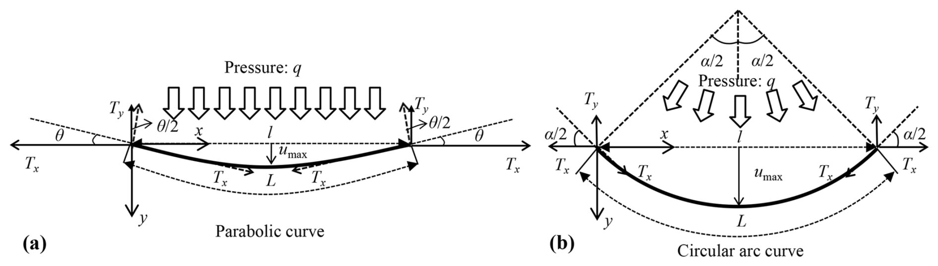
Figure A1 Deformation assumption of the cable subjected to normal debris-flow loading. Note that the calculation of the tensile force here is different from that in (Brighenti et al., 2013; Song et al., 2018, 2019) due to the setting of pulleys at the extremities of the cable.

As for the load hypothesis, a general consensus consists in considering a uniform distribution along the barrier length. By comparison with other distributions (triangular or parabolic), this distribution was in particular considered more appropriate for the static load estimation (Wendeler, 2008; Wendeler et al., 2019). As for the second hypothesis, the barrier deformation along the channel transverse axis is either considered circular or parabolic. In the first case, the loading is considered normal to the deformed barrier (Song et al., 2018, 2019) while in the second case, it is considered parallel to the channel direction (Brighenti et al., 2013; Wendeler et al., 2019; Huo et al., 2023). Both these shapes were considered in this study and their results were compared.

From the pattern of the parabolic curve depicted in Fig. A1a, the deflection along the barrier length u(x) of a given cable in the flow direction is expressed as follows:

$$\begin{array}{}\text{(A1)}& u\left(x\right)={\displaystyle \frac{q}{\mathrm{2}{T}_x}}(x\cdot l-x^{\mathrm{2}})\end{array}$$

where q is the uniformly distributed load (N m⁻¹) along the initial length of the cable l and T_x is the component of the tensile force T along the x-axis. The maximum deflection u_max is observed at the centre point of the cable and is given by:

$$\begin{array}{}\text{(A2)}& u_{\max }=u\left(x={\displaystyle \frac{l}{\mathrm{2}}}\right)={\displaystyle \frac{q{l}^{\mathrm{2}}}{\mathrm{8}{T}_x}}\end{array}$$

From the elongation of the cable Δl and ignoring the higher differentiation, the maximum deflection u_max can be calculated using:

$$\begin{array}{}\text{(A3)}& L-l=\mathrm{\Delta }l={\displaystyle \frac{\mathrm{8}{u}_{\max }^{\mathrm{2}}}{\mathrm{3}l}}\end{array}$$

where L is the length of cable once deformed with a parabolic shape. Therefore, the deflection angle at one cable's extremity, θ, is obtained by solving the derivative of the curve along the barrier length at the cable's extremity:

$$\begin{array}{}\text{(A4)}& \tan \mathit{\theta }={\displaystyle \frac{\mathrm{d}u}{\mathrm{d}{x}_{|x=\mathrm{0}}}}={\displaystyle \frac{ql}{\mathrm{2}{T}_x}}={\displaystyle \frac{\mathrm{4}{u}_{\max }}{l}}\end{array}$$

Combining Eqs. (A4), (A2) and (A3), it comes:

$$\begin{array}{}\text{(A5)}& \tan \mathit{\theta }={\displaystyle \frac{\mathrm{2}}{l}}\sqrt{{\displaystyle \frac{\mathrm{3}l\cdot \mathrm{\Delta }l}{\mathrm{8}}}}\end{array}$$

The normal load acting on total on the cable, F_n is obtained from:

$$\begin{array}{}\text{(A6)}& F_n=\mathrm{2}{T}_y=\mathrm{4}{T}_x\sin {\displaystyle \frac{\mathit{\theta }}{\mathrm{2}}}\cos {\displaystyle \frac{\mathit{\theta }}{\mathrm{2}}}=\mathrm{2}{T}_x\cdot \sin \mathit{\theta }\end{array}$$

As such F_n is back-calculated depending on the tensile force measurement and the elongation Δl. It is noteworthy that in this study the barrier cables are deviated by pulleys in such a manner that T_x is obtained from the force sensors.

For the circular assumption (Fig. A1b), the load is uniformly perpendicular to the deformed cable. According to Song et al. (2019), the form finding of the cable is explicitly based on the curvature angle of the circular arc α_i and the arc length L. α can be related to the initial and arc length of the cable by the Taylor expansion as Sasiharan et al. (2006):

$$\begin{array}{}\text{(A7)}& {\displaystyle \frac{\mathit{\alpha }}{\mathrm{2}}}=\sqrt{\mathrm{6}\left(\mathrm{1}-{\displaystyle \frac{l}{L}}\right)}\end{array}$$

Here the deflection angle θ is equal to $\mathit{\alpha }/\mathrm{2}$, yielding the same calculation expressed by Eq. (A6). The maximum deflection can be calculated by:

$$\begin{array}{}\text{(A8)}& u_{\max }={\displaystyle \frac{\mathrm{0.5}l}{\sin (\mathit{\alpha }/\mathrm{2})}}[\mathrm{1}-\cos (\mathit{\alpha }/\mathrm{2}\left)\right]\end{array}$$

Then, F_n is computed using Eq. (A6) substituting θ with $\mathit{\alpha }/\mathrm{2}$.

For both deformed shape assumptions, F_b is computed as the sum of the F_n values obtained for the three cables.