Severe beach erosion induced by shoreline deformation after a large-scale reclamation project for the Samcheok liquefied natural gas (LNG) terminal in South Korea

Large-scale construction projects, such as port construction and reclamation endeavors, can alter inshore wave dynamics, leading to severe coastal erosion. In South Korea, recent large-scale reclamation projects have resulted in severe sand erosion along nearby coastlines. This study focused on Wolcheon Beach, where complete sand loss had occurred due to robust long-shore sediment transport (LST) induced by a reclamation project for construction of the nearby Samcheok liquefied natural gas terminal in Gangwon Province. A shoreline change model was employed to simulate this phenomenon, and the results were validated using satellite imagery. Model accuracy was assessed by comparing the LST rate vectors indirectly estimated from the changes in the shoreline delineated in the satellite images with those directly derived from the model. Furthermore, a response methodology was proposed using the parabolic bay-shaped equation, which can effectively mitigate coastal erosion by controlling LST by installing a small-scale groin group on the adjacent beach before commencing reclamation or port projects. These findings are expected to contribute significantly to averting catastrophic coastal erosion issues, such as those witnessed at Wolcheon Beach, before large-scale construction in coastal regions is performed.

1 Introduction

Coastal areas are inhabited by nearly half of the global population and are much more densely populated than inland areas, although they occupy only a small fraction of the Earth's surface. Approximately two-thirds of the world's megacities are situated within 60 km of shorelines, with immense economic significance for marine transportation, fishing, and tourism (Neumann et al., 2015). Ports facilitate 80 %–90 % of global trade, and many individuals choose coastal regions as vacation destinations (Notteboom and Rodrigue, 2005). Coastal zones are increasingly serving as leisure and cultural hubs, making effective coastal management imperative. Although coastal development provides economic benefits, it can profoundly impact the environment and ecosystems. Coastal development, such as harbor and fishing port reclamations, exacerbates erosion through various mechanisms. Altering natural ecosystems and coastal topography leads to sediment displacement by wave action and nearshore currents, resulting in coastal erosion.

Coastal erosion is emerging as a global problem, as indicated by several studies. Climate change is causing sea levels to rise, and coastal erosion has become a new environmental problem. The rates of coastal loss due to sediment transport are increasing annually, which is critical for highly exposed coastal cities and coral islands that are vulnerable to erosion (Ortega et al., 2023; Parvathy et al., 2023). As technology develops and data accumulate, remote sensing has become an effective means of analyzing coastal erosion. Remote-sensing technology allows the collection and analysis of high-resolution images through a variety of platforms, including satellites, aircraft, and drones, allowing real-time monitoring of shoreline changes and precise analysis of past erosion levels and patterns (Nativí-Merchán et al., 2021). Several erosion mitigation measures are also being continuously devised to counter shoreline deformation induced by coastal development or sea-level rise. Beach nourishment, which involves the supplementation of substantial amounts of sand to preserve the original beach, is a common practice, along with installation of coastal structures such as detached breakwaters or groins. However, implementing inappropriate coastal structures can exacerbate erosion. For example, the double-headland method was employed to counteract sand loss at Yeongrang Beach, the city of Sokcho, in Gangwon Province. However, as noted by Lim et al. (2021), this resulted in excessive beach distribution by diffraction waves, which impeded the intended erosion reduction function of the coastal structure.

Wave deformation caused by coastal structures mainly influences long-shore sediment transport (LST), leading to shoreline reshaping (Lim et al., 2021). Numerous studies have elucidated sediment transport in coastal areas due to wave action and established theoretical formulas for coastal erosion. Pelnard-Considère (1957) proposed a governing equation in which the shoreline position was determined by LST along the coast. This equation is based on the assumptions that sediment does not alter the beach profile and that the active profile of the beach uniformly advances or retreats in the transverse direction. In reality, while cross-shore sediment transport can play a role, LST, driven by changes in the nearshore wave field, is generally considered more influential in shaping shoreline changes over extended periods. Predictions of shoreline changes using only empirical formulas for LST are limited by the complex causes of shoreline alterations caused by ports and coastal structures. For example, during storm events, wave breaking suspends beach sand, leading to significant short-term erosion in the lateral direction. Yates et al. (2009) investigated the shoreline equilibrium on coasts eroded by suspended sediments under constant wave energy influx using field observation data. Although long-term field observations yield insightful results, Kim et al. (2021) proposed a simple method that achieved similar outcomes, by applying an empirical formula for equilibrium beach profiles. When wave activity subsides after a storm, suspended sand settles, forming berms and restoring the original coastline. Lim et al. (2022a) and Lim and Lee (2023) derived governing equations for simulating both long- and short-term shoreline erosion caused by LST, by analyzing short-term coastal erosion along with the horizontal behavior of suspended sediments.

Despite several limitations, the one-line shoreline change model introduced by Pelnard-Considère (1957) specializes in simulating temporal shoreline changes due to groin installation (Le Mehaute and Soldate, 1979; Walton and Chiu, 1979; Hanson, 1989). However, the original version of the model did not consider wave diffraction effects caused by large or detached breakwaters. Consequently, efforts have been made to enhance the model for scenarios where wave diffraction from coastal structures is significant. Various numerical (Hanson, 1989; Leont'yev, 1997, 2007) and mathematical (Vaidya et al., 2015) approaches have been proposed that are primarily based on empirical formulas. The GENESIS model proposed by Hanson (1989) incorporates the impact of coastal structures on shoreline changes by introducing an additional term for long-shore variation in the breaking-wave height, as presented by Ozasa and Brampton (1980). Although this model is widely used in engineering, it underestimates results in scenarios involving wave diffraction from large-scale coastal structures (Lee and Hsu, 2017).

Recently, Lim et al. (2021) developed a shoreline change model by applying the empirical equilibrium shoreline formula proposed by Hsu and Evans (1989) to reflect wave diffraction from capes, bays, and artificial structures. The planform of the static equilibrium shoreline exhibits a certain form owing to the shoreline equilibrium on a mobile sand bed, and numerous empirical studies have been conducted for its prediction (Hsu and Evans, 1989; Moreno and Kraus, 1999; Yasso, 1965). The parabolic bay shape equation (PBSE) proposed by Hsu and Evans (1989) has been globally adopted for coastal management owing to its efficacy (González and Medina, 2001; Herrington et al., 2007; Bowman et al., 2009; Silveira et al., 2010; Yu and Chen, 2011). Lim et al. (2019) demonstrated the applicability of the PBSE to the East Sea shoreline of South Korea using East Sea wave data. To address control point uncertainty of the PBSE defined in orthogonal coordinate systems, Lim et al. (2022b) supplemented it for application to cylindrical coordinates.

The present study investigated the complete disappearance of sand on Wolcheon Beach within 1 year due to LST following a considerable change in the wave field resulting from large-scale reclamation on Hosan–Wolcheon beaches near Samcheok, South Korea, to construct a liquefied natural gas (LNG) pier. The shoreline change model developed by Lim et al. (2021), which comprises three main parts, was employed for the analysis. First, information on the Samcheok LNG terminal and Wolcheon Beach (i.e., the study area) was introduced, and rapid shoreline changes on Wolcheon Beach were delineated from satellite images using Google Earth Engine. Subsequently, the results of the numerical coastal erosion simulation model were compared with the satellite analysis results. Finally, the LST rate was examined using the shoreline change results and compared with the empirical formula of the Coastal Engineering Research Center (CERC).

As previously stated, the applied numerical model is an enhanced shoreline change model based on the PBSE (Lim et al., 2021). The model was refined to incorporate the influences of diffraction waves caused by significant coastal structures. This case study underscores the importance of assessing changes in nearby shorelines before conducting large-scale coastal construction projects, thereby providing insights into methods that minimize potential damage. The impact of groin installation on controlling coastal sediment was simulated numerically, highlighting the necessity of such experiments when predicting changes in the wave field. Consequently, this study investigated the ramifications of harbor and fishing port development, as well as large-scale reclamation, which can alter wave fields in coastal regions during rapid and catastrophic erosion.

2 Study site

2.1 Location of Wolcheon Beach

Wolcheon Beach is located in Samcheok, Gangwon Province, South Korea. Hosan Beach, where the Samcheok LNG terminal was constructed, is located north of Gagok Creek. Wolcheon Beach, which is the main one to have suffered erosion damage, is located to the south of the creek. Hosan Beach is located to the south of Hosan Creek and forms an almost straight 1.91 km shoreline along Wolcheon Beach.

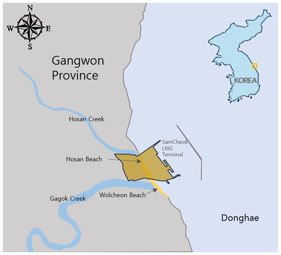
Figure 1 Study site location including Hosan and Wolcheon beaches and the Samcheok LNG terminal. On the map, Korea refers to the Korean Peninsula.

2.2 Overview of the Samcheok LNG terminal development

The Samcheok LNG terminal is the fourth largest natural gas production facility in South Korea after the Pyeongtaek, Incheon, and Tongyeong terminals. It was constructed from 2010–2017 to ensure a stable gas supply to the Gangwon and Yeongnam regions. The marine site has a total area of approximately 980 000, of which 590 000 m² is occupied by the marine site. The marine site was completed in 2011, and 12 LNG storage tanks (three 270 000 and nine 200 000 kL tanks) were installed at the site. In addition, docking facilities for 200 000 t LNG ships and a trade port with a 1800 m breakwater (i.e., the largest in South Korea) were developed.

As shown in Fig. 2a, Wolcheon Beach was well preserved in a direction perpendicular to the dominant direction of the wave incidence in 2011. In 2012, however, all the sand on the approximately 40 m wide beach was lost due to severe beach erosion caused by the wave field change, as shown in Fig. 2b. This has become a major social issue because of the serious overtopping and erosion damage that occurred in nearby villages and has prompted the introduction of laws and systems to assess of the effects of beach erosion in advance when coastal area development (e.g., reclamation and port construction) is planned. Lim et al. (2021) revealed that the erosion of Wolcheon Beach was caused by the reclamation project of the Samcheok LNG terminal and the outer breakwater. They showed this by applying a shoreline change model, which was established by applying the PBSE of Hsu and Evans (1989) to cylindrical coordinates.

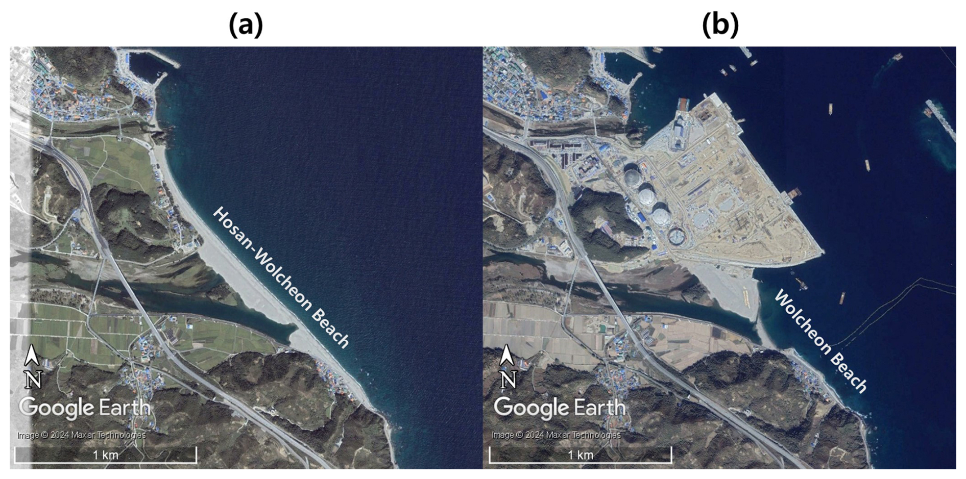
Figure 2 Aerial photographs of Hosan–Wolcheon beaches before construction of the Samcheok LNG terminal: (a) June 2011 and (b) October 2012 (© Google Earth).

2.3 Wave and coastal environment of Wolcheon Beach

The coastal waters near the Samcheok LNG terminal, where Wolcheon Beach is located, have depths ranging from approximately 20 to 30 m. These waters are exposed to moderate-wave-energy to high-wave-energy conditions, with a mean annual significant wave height between approximately 1.04 and 1.24 m. The coastline is elevated, long, and straight due to the dominant wave direction approaching almost perpendicularly to the shore. Regarding the incident wave on Wolcheon Beach, the root mean square wave height is estimated to be 1.14 m, as can be seen from the National Oceanic and Atmospheric Administration (NOAA) data in Fig. 3. Figure 3 also shows that the wave climate, which is one of the main causes of beach erosion, did not change significantly in Samcheok. The NOAA data site (37.0° N, 129.5° E) is located 27 km from Wolcheon Beach. Figure 4 shows the wave rose (blue) in deep water obtained from the wave hindcasting data and the resulting rose diagram of the LST components (green: north; orange: south). The angle shown in Fig. 4 represents the wave direction with respect to the wave increase. The dominant direction of wave incidence for the static equilibrium of Wolcheon Beach was 34.2° N from true north. Figure 4 also shows the littoral rose according to the wave rose, drawn symmetrically around the vertical line in the dominant direction (124.2–304.2° N). The static equilibrium shoreline was considered to occur at an angle at which LST was balanced. The direction of the static equilibrium shoreline maintained an angle of approximately 90° with the dominant direction of wave incidence in the absence of the net transport component of LST.

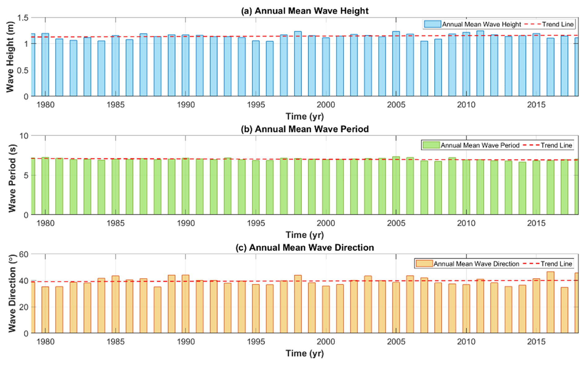
Figure 3 Changes in the annual mean (a) wave height, (b) wave period, and (c) wave direction obtained from NOAA wave data near Wolcheon Beach.

Figure 4 Combined rose diagram of wave and littoral drift for the study site.

In addition, the tidal range is small in Samcheok coastal waters (≤ 30 cm). Because of their small tidal range, beaches are usually affected by wave-induced currents rather than by tidal currents. The mean sea level (S0), which is the sum of the four major partial tides in the waters near Hosan Port, was low (18.4 cm). The tide form number (i.e., the ratio of the diurnal tide semi-tidal range [K1 + O1] to the semidiurnal tide semi-tidal range [M2 + S2]) was 1.45 cm, indicating that the semidiurnal tide was dominant and that two high tides and two low tides occurred daily. The impact of the tidal current was not significant as the tidal range was approximately 0.3 m. Southward flow was observed during the flood tide and northward flow during the ebb tide at rates ranging from 0.1–0.4 m s⁻¹.

3 Beach survey data

3.1 Global positioning system shoreline survey

Analysis of data from the shoreline survey conducted six times from April 2010 to December 2011 (during which time there was rapid shoreline changes) revealed that the beach width increased to 60 m in the baseline 04 section of the Hosan–Wolcheon beaches (Fig. 5); however, it decreased by > 90 % in the baseline 05 and 06 sections where Wolcheon Beach was located.

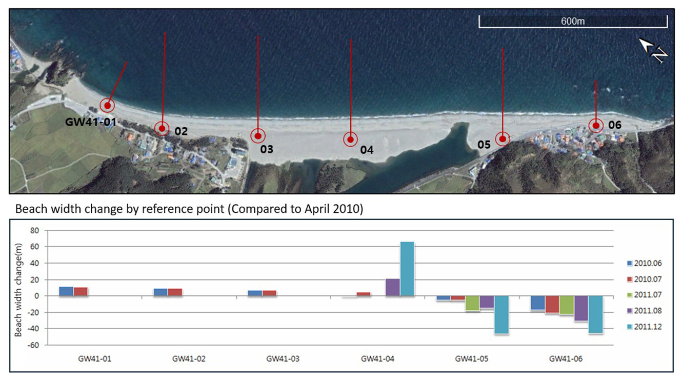
Figure 5 Beach width change by reference point on Hosan–Wolcheon beaches (source: GSESRH, 2013; © Google Earth).

3.2 Survey of sand characteristics

Sand grain size on a beach is an important physical variable used to determine the LST rate, which is determined by the action of wave energy on the coast. After construction of the Samcheok LNG terminal, most of the sand on Wolcheon Beach was introduced into the Gagok Creek estuary in 2012 (Fig. 6a). Figure 6b shows the cumulative sand grain size distribution surveyed during this period. The median grain size of sand (D₅₀) was 0.666 mm. The porosity and specific gravity of the sand were also required to determine the LST rate. Owing to the absence of data for the target area, values of porosity, p =0.42, and sand gravity weight, s =2.65, were applied, as these are representative values for South Korea.

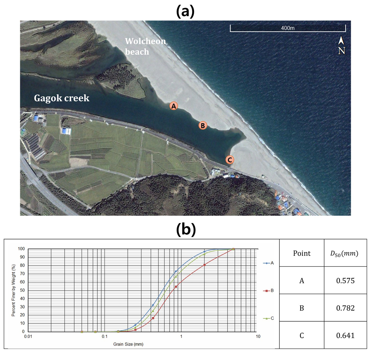
Figure 6 (a) Sand collection location and (b) survey results for cumulative grain size curves and median grain sizes for sand (D₅₀) at Gagok Creek estuary (source: GSESRH, 2013; © Google Earth).

3.3 Analysis of shoreline data acquired from satellite images

To identify rapid shoreline changes on Wolcheon Beach from 2011–2012, Landsat 7 images from the Google Earth Engine platform were used. Landsat 7, launched in 1999, is managed by the United States Geological Survey. The Landsat series captures high-resolution multispectral images of the Earth's surface and provides important information for various fields including environmental monitoring, natural disaster monitoring, agriculture, forest management, and urban development. The series have red, blue, green, near-infrared, and medium-infrared spectral bands with a 30 m spatial resolution. The red–green–blue images at 10 time points in which changes in the shoreline could be observed were selected (Fig. 7). Several authors (Baghdadi et al., 2004; Modava and Akbarizadeh, 2017; She et al., 2017; Vos et al., 2019; Bengoufa et al., 2021) have successfully used satellite images to extract shorelines. However, as highlighted by Liu and Jezek (2004), shoreline extraction often requires rigorous terrain correction, geocoding, radiometric correction, and balancing.

As shown in Fig. 7, the repeated occurrence of black bands that prevented the images from being read made it difficult to process most of the images using conventional shoreline extraction methods; therefore, the images were extracted using a direct digitization method. The LNG terminal revetment and extracted shorelines are also shown in the corresponding satellite imagery (Fig. 7). The entire extracted shoreline is shown in the last satellite image in Fig. 8 from the shoreline on 13 March 2011 (i.e., before the LNG project began) to 12 December 2012 (i.e., approximately 21 months later). In < 2 years, an average of 37 m of beach erosion occurred at Wolcheon Beach, whereas a shoreline advance of 145 m occurred along the LNG terminal revetment.

Figure 7 Satellite images of Landsat 7 selected for Wolcheon Beach shoreline analysis from 2011–2012 and extracted shorelines: (a) 13 March 2011, (b) 5 September 2011, (c) 24 November 2011, (d) 26 December 2011, (e) 11 January 2012, (f) 12 February 2012, (g) 31 March 2012, (h) 18 May 2012, (i) 6 August 2012, and (j) 12 December 2012 (© Google Earth).

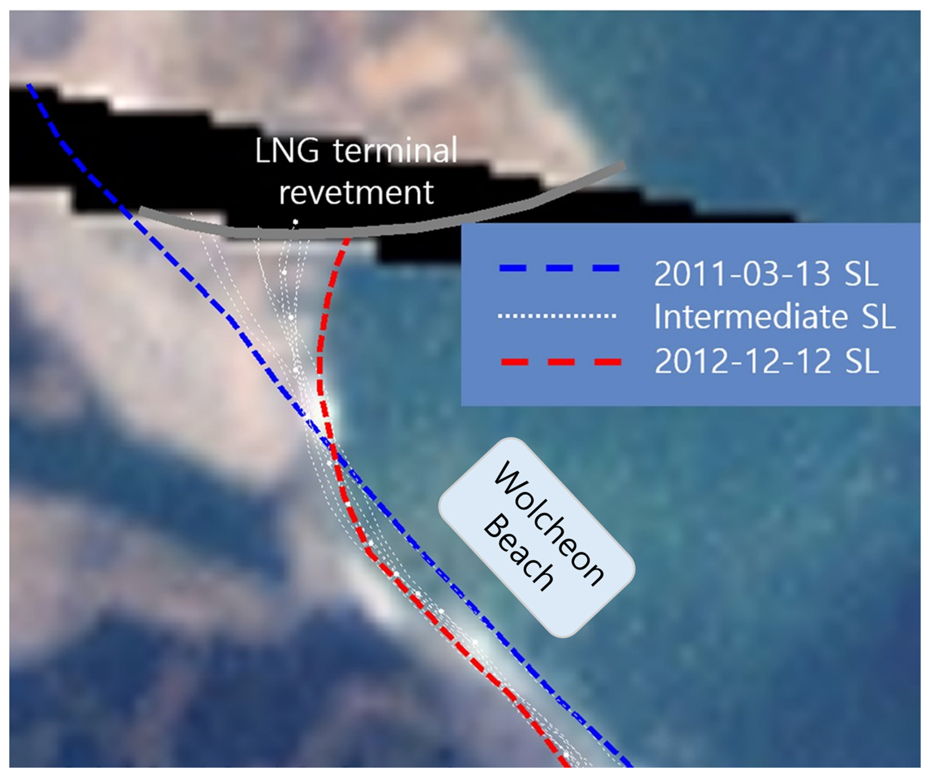
Figure 8 Shoreline changes from Landsat 7 satellite images of Wolcheon Beach from 2011–2012 (© Google Earth).

4 Numerical simulation of shoreline change

4.1 Governing equation

In this study, we employed one of the currently available shoreline change models that can simulate temporal changes in the shoreline extracted from satellite images. Recently, Lim et al. (2021) extended the governing equation first proposed by Pelnard-Considère (1957) to cylindrical coordinates, as given below, for application to concave coasts.

$$\begin{array}{}\text{(1)}& {\displaystyle \frac{\partial r_{\mathrm{s}}}{\partial t}}+{\displaystyle \frac{\mathrm{1}}{(h_{\mathrm{c}}+h_{\mathrm{B}})}}{\displaystyle \frac{\partial Q_{\mathrm{l},\mathit{\theta }}}{r_{\mathrm{s}}\partial \mathit{\theta }}}=\mathrm{0},\end{array}$$

where r_s is the distance from the center of the circumference to the shoreline, which decreases and increases when the shoreline advances and retreats, respectively; θ represents the coordinates in the shoreline direction; h_B and h_c are the berm height and closure depth, respectively; and Q_l,θ is the LST rate in the θ direction. To consider the wave diffraction effect caused by the presence of structures, the LST rate equation can be modified based on the CERC (1984) as follows.

$$\begin{array}{}\text{(2)}& Q_{\mathrm{l},\mathit{\theta }}=C^{\prime }{H}_{\mathrm{b}}^{\frac{\mathrm{5}}{\mathrm{2}}}\sin \mathrm{2}\left({\mathit{\alpha }}_{\mathrm{m}}-{\mathit{\alpha }}_{\mathrm{e}}\right),\end{array}$$

where H_b is the breaking-wave height, α_m is the annual mean wave angle, and α_e is the equilibrium planform gradient which can be estimated based on the approximate PBSE. In Eq. (2), C^′ is a constant and is calculated as follows:

$$\begin{array}{}\text{(3)}& C^{\prime }={\displaystyle \frac{K\sqrt{g/\mathit{\kappa }}}{\mathrm{16}(s-\mathrm{1})(\mathrm{1}-p)}},\end{array}$$

where K is the coastal sediment coefficient, which can range from 0.04–1.1 depending on sediment transport. Komar and Inman (1970) proposed K has a value of 0.77. s and p represent the sediment specific weight and sediment porosity, respectively.

4.2 Estimation of initial LST by PBSE

When a structure such as a breakwater or groin is installed on the shore, the equilibrium shoreline changes, and LST is generated towards the structure. As shown in Eq. (2), LST has a maximum value when (α_m − α_e) is 45° (degree units). Since α_m is initially 0°, the maximum LST value will initially be shown at the shoreline location where α_e becomes 45°. In Eq. (2), the equilibrium planform gradient α_e can be obtained from the approximate expression of PBSE given below (Fig. 9).

$$\begin{array}{}\text{(4)}& R\cong {\displaystyle \frac{a}{\sin \mathit{\beta }}}{\displaystyle \frac{\mathit{\beta }}{{\mathit{\theta }}_{\mathrm{e}}}},\end{array}$$

where a denotes the vertical distance between the wave crest baseline passing through the focus point and the shore baseline passing through the downdrift control point X (i.e., down-coast limit), θ_e is the angle between the wave crest baseline and the line connecting the parabolic focus to the equilibrium shoreline, and β is the reference wave angle at the downdrift control point.

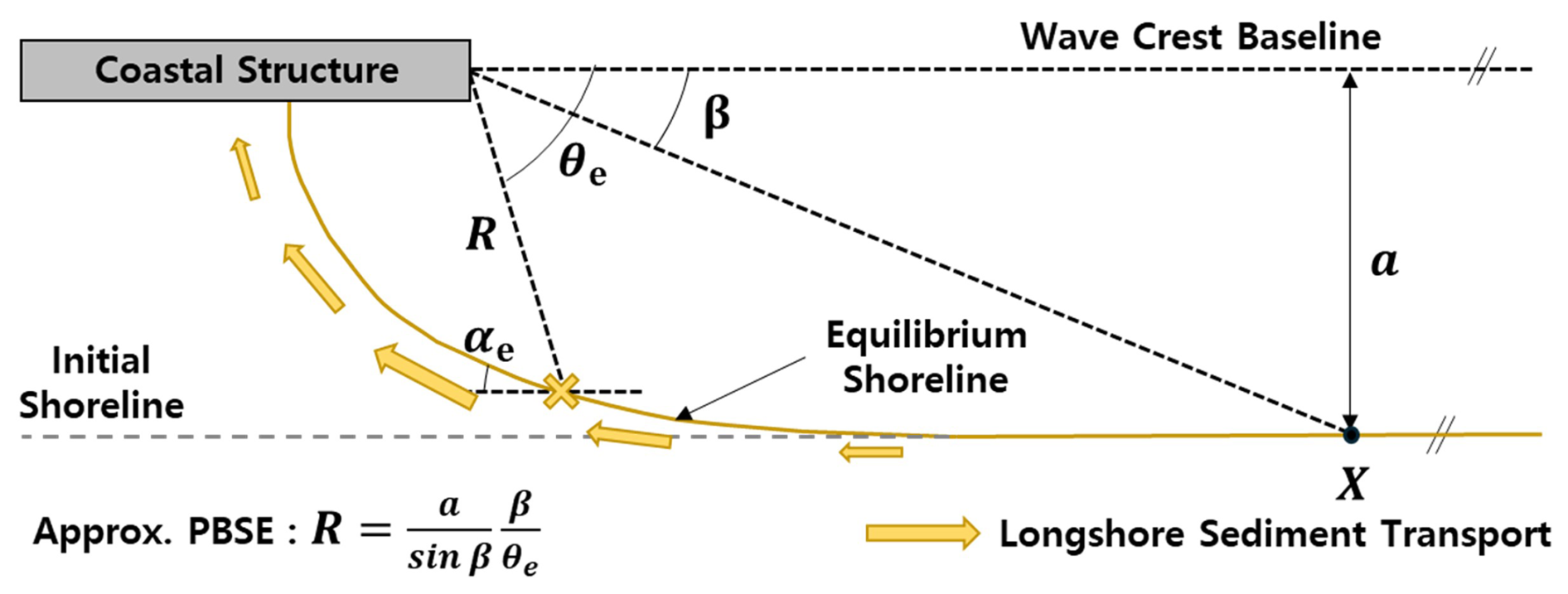
Figure 9 Definition sketch for estimation of initial LST owing to coastal structure construction.

If the coast is ultimately eroded due to LST, it can be assumed that the θ_e at which erosion occurs on the coast becomes β. Therefore, θ_e can be obtained from the straight distance, R, between the focus and the grid point of the θ cell, as shown in Eq. (5).

$$\begin{array}{}\text{(5)}& {\mathit{\theta }}_{\mathrm{e}}\cong {\tan }^{-\mathrm{1}}\left({\displaystyle \frac{a}{R}}\right)\end{array}$$

The α_e can be estimated based on the approximate PBSE according to θ_e, using the following equation.

$$\begin{array}{}\text{(6)}& {\mathit{\alpha }}_{\mathrm{e}}={\tan }^{-\mathrm{1}}\left({\displaystyle \frac{\sin {\mathit{\theta }}_{\mathrm{e}}-{\mathit{\theta }}_{\mathrm{e}}\cos {\mathit{\theta }}_{\mathrm{e}}}{\cos {\mathit{\theta }}_{\mathrm{e}}+{\mathit{\theta }}_{\mathrm{e}}\sin {\mathit{\theta }}_{\mathrm{e}}}}\right)\end{array}$$

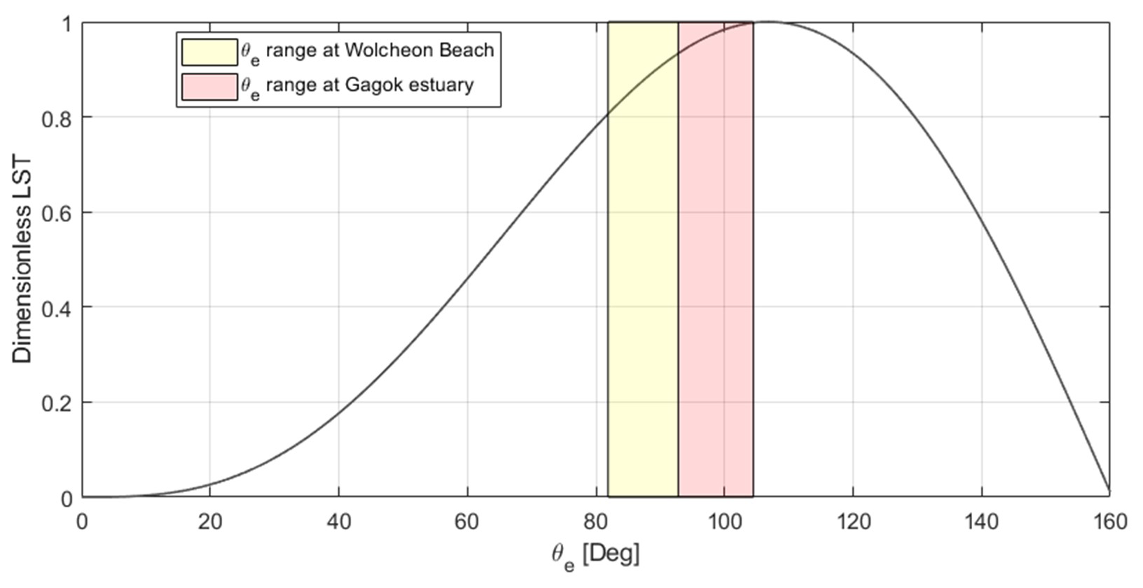
Figure 10 shows the dimensionless initial LST ($Q_{\mathrm{l},\mathit{\theta }}/\left[C^{\prime }{H}_{\mathrm{b}}^{\frac{\mathrm{5}}{\mathrm{2}}}\right]$) according to α_e obtained by applying Eq. (6) to the CERC equation after coastal structure installation. In the case of Wolcheon Beach where θ_e ranged from 81.9–92.8°, the dimensionless initial LST ranged from 0.807–0.933, indicating that installation of the Samcheok LNG terminal may cause serious erosion due to LST in the Wolcheon Beach area. In particular, in the Gagok Creek estuary where θ_e ranged from 92.8–104.5°, the calculated dimensionless initial LST ranged from 0.933–0.998, making it an area where shoreline deformation due to serious LST differences is unavoidable.

Figure 10 Dimensionless initial LST ($Q_{\mathrm{l},\mathit{\theta }}/\left[C^{\prime }{H}_{\mathrm{b}}^{\mathrm{5}/\mathrm{2}}\right])$ according to the shoreline location angle θ_e.

4.3 Numerical scheme

The governing equation of the shoreline change model was solved using the finite-difference method. The beach is divided into Δθ grids along the coast, and it is assumed that sediment transport in the zone increases or decreases depending on the sediment loss or inflow by grid along the coast. A staggered grid system is used, in which {r_s} and {Q_l,θ} are defined alternatively in odd–even order (i represents the grid number). Q_l,θ, the sediment transport along the long-shore grid, was defined as being located at the boundary of each grid, while the shoreline position was defined to be located at the center of the grid. To express the finite-difference equation conveniently, the superscript n+1 denotes the value to be obtained at the next time step, and n is defined as the value already calculated at the present time step. Therefore, $r_{\mathrm{si}}^{n+\mathrm{1}}$, which is the shoreline position of the ith grid at the next time step, n+1, can be expressed using Eq. (7):

$$\begin{array}{}\text{(7)}& r_{\mathrm{si}}^{n+\mathrm{1}}=r_{\mathrm{si}}^n+{\displaystyle \frac{\mathrm{\Delta }t}{h_{i,j}}}\left({\displaystyle \frac{Q_{\mathrm{l},\mathit{\theta }i+\mathrm{1}}-Q_{\mathrm{l},\mathit{\theta }i}}{r_{\mathrm{si}}\mathrm{\Delta }\mathit{\theta }}}\right),\end{array}$$

where Δt is the time step and Δθ is the shoreline grid. The LST rate that converges to the equilibrium can be calculated using Eq. (7). As previously explained, the explicit-scheme method is used to obtain the newly determined shoreline position using past values.

The erosion control line is the boundary condition on the shore side in the transverse direction. When the shoreline met the hard boundary (i.e., the erosion control line) due to erosion progression, the complete loss of beach sand was assumed for no further long-shore sediment generation and no further shoreline retreat.

5 Application to severe beach loss event on Wolcheon Beach

5.1 Review of changes in equilibrium shoreline after Samcheok LNG reclamation

The Samcheok LNG terminal near the study site was constructed after large-scale reclamation, which changed the equilibrium shoreline (Fig. 11). The equilibrium shoreline was estimated using MeePaSoL, as described by Lim et al. (2022b), which is a MATLAB GUI tool. After reclamation, the equilibrium shoreline changed (as marked in green) owing to changes in the wave environment. This corresponds to the shoreline being newly formed on equilibrium if it was composed of sand. Therefore, the sand on the sea side of this line was subjected to LST towards the Gagok Creek estuary owing to nearshore current circulation induced by diffracted waves that carry sediment.

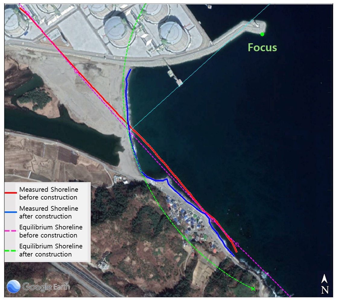
Figure 11 Change in equilibrium shoreline after reclamation estimated using MeePaSoL (© Google Earth).

5.2 Numerical-simulation conditions

According to the information obtained through the shoreline analysis (Sect. 3.3), the shoreline began to change from March–September 2011. Through several simulations, the most similar start time for shoreline change was found in the numerical model and satellite data analysis results. Therefore, it was inferred that shoreline deformation began on 17 August 2011. Table 1 lists the values used in numerical simulations. A numerical simulation was performed for a wave height, H, of 1 m and wave period, T, of 5 s, under normal wave conditions. This is because the shoreline change due to the wave diffraction effect caused by coastal structures, rather than by deformation by high waves, continued for long periods with a low wave height.

Figure 12 shows the area and grid information applied to the numerical model. The coordinates of the origin of the cylindrical coordinate system are 37°11^′49^′′ N and 129°23^′45^′′ E, and the radius for fitting the shoreline of Hosan–Wolcheon beaches is R=5.270 km. The computing area was composed of 50 grids at Δθ=0.2176° intervals along the 1.0 km long beach zone from θ_s=81.9° to θ_e=92.8° with respect to true north for the center of the circle that fitted the original shoreline. At the points where the shoreline is located, Δθ corresponds to a 20 m length. The southeastern boundary has a boundary condition wherein sand inflow and outflow are free, and an impermeable boundary condition is applied along the LNG revetment.

Table 1 Values applied in numerical simulation.

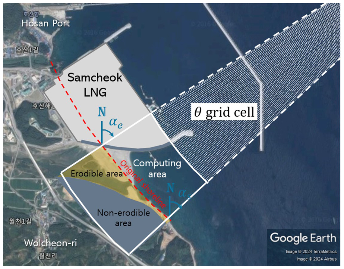
Figure 12 Grid system of cylindrical coordinates for shoreline change numerical simulation (© Google Earth).

5.3 Numerical-simulation results and verification

5.3.1 Shoreline change prediction results

It was assumed that the shoreline change began in August 2011, when the revetment for the Samcheok LNG terminal reclamation was completed, and the numerical simulation was performed until December 2012, when no further significant changes were observed. Assuming that the seabed contours are straight and parallel, the NOAA wave climate dataset is converted to breaking waves. A value of approximately 0.1782 is generated for C^′ under the application of the coastal sediment coefficient K= 0.77, wave breaking coefficient κ= 0.78, sediment specific weight s= 2.57, and porosity p= 0.39, which are applied to the typical sediment transport rate. On the east coast of South Korea, the specific gravity s= 2.65 and porosity p= 0.42 were obtained on average; therefore, $C^{\prime }=$ 0.1783, which is a commonly used value.

The numerical model results are displayed as dashed yellow lines in the satellite images in Fig. 13, and the grey line represents the revetment. In the numerical simulation, the shoreline did not change when it reached the revetment. Overall, the shorelines recognized from the satellite images are similar to the numerical-simulation results. Because the grid size of the numerical model was 20 m, satellite data were interpolated at the same intervals. Figure 14 shows the shoreline changes extracted from satellite images from 3 March 2011 to 12 December 2012 on the satellite image from 12 December 2012. On average, 22 m of beach erosion occurred in the Wolcheon Beach erosion area, and a maximum shoreline advance of 102 m occurred at the LNG terminal revetment. The numerical results are underestimated compared with the values obtained from satellite images. Figure 15 shows a comparison of the numerical calculations with the values obtained from satellite images.

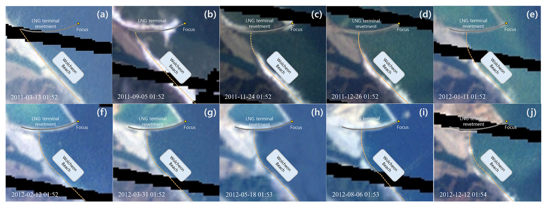
Figure 13 Comparison between the predicted shoreline change model results and the shoreline extracted from satellite images: (a) 13 March 2011, (b) 5 September 2011, (c) 24 November 2011, (d) 26 December 2011, (e) 11 January 2012, (f) 12 February 2012, (g) 31 March 2012, (h) 18 May 2012, (i) 6 August 2012, and (j) 12 December 2012 (© Google Earth).

Figure 14 Numerical results of shoreline changes on Wolcheon Beach from 13 March 2011 to 12 December 2012 (© Google Earth).

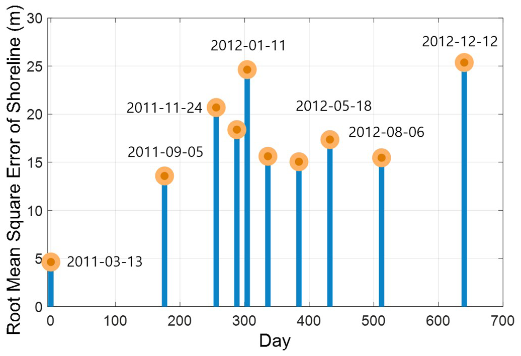
Figure 15 Temporal variation in root mean square errors between the shoreline obtained from satellite images and the predicted shoreline results.

5.3.2 Comparison through LST rate vectors

This section presents the results of LST rate generation from shoreline changes extracted from satellite images. Similar research has been conducted on the analysis of sediment transport (Jung et al., 2004; Rahmawati et al., 2021; Lim et al., 2024). The results of Eq. (8), obtained from the finite-difference equation of the shoreline change model, are obtained from the shoreline data at two adjacent time points. In this study, the shoreline change by grid was estimated from coastal observation data by applying the formula proposed by Jung et al. (2004) to the shoreline data, which were modified to maintain the beach area based on the sediment mass conservation rule.

Jung et al. (2004) presented a method of estimating the LST rate Q_l,i under the given shoreline change width, Δy_i, as shown in Eq. (8). Accordingly, the LST rate during the shoreline survey period, Δt, is calculated.

$$\begin{array}{}\text{(8)}& {\mathit{Q}}_{\mathrm{l},i+\mathrm{1}}-{\mathit{Q}}_{\mathrm{l},i}=\mathrm{\Delta }x{D}_s{\displaystyle \frac{\mathrm{\Delta }{y}_i}{\mathrm{\Delta }t}}=C\mathrm{\Delta }{y}_i=\stackrel{\mathrm{´}}{C_i},\end{array}$$

where $C=\mathrm{\Delta }x{D}_s/\mathrm{\Delta }t$ and $D_s=h_{\mathrm{c}}+h_{\mathrm{B}}$. Thus, if $C_i{}^{\prime }=\mathrm{\Delta }x{D}_s\mathrm{\Delta }{y}_i/\mathrm{\Delta }t$ holds and the upstream LST rate Q₁ is known, a matrix equation to estimate the LST rate Q_l,i is derived as follows.

$$\begin{array}{}\text{(9)}& \begin{array}{rl}& \left[\begin{array}{llllll}\mathrm{1}& & & & & \\ -\mathrm{1}& \mathrm{1}& & & & \\ & & :& & & \\ & & & -\mathrm{1}& \mathrm{1}& \\ & & & & -\mathrm{1}& \mathrm{1}\end{array}\right]\left[\begin{array}{l}{Q}_{\mathrm{l},\mathrm{2}}\\ Q_{\mathrm{l},\mathrm{3}}\\ :\\ Q_{\mathrm{l},N}\\ Q_{\mathrm{l},N+\mathrm{1}}\end{array}\right]\\ & =\left[\begin{array}{l}{C}_{\mathrm{2}}^{\prime }+Q_{\mathrm{l},\mathrm{1}}\\ C_{\mathrm{2}}^{\prime }\\ :\\ C_{N-\mathrm{1}}^{\prime }\\ C_N^{\prime }\end{array}\right]\end{array}\end{array}$$

Model results are validated by comparing them with the vectors obtained from the numerical model results. Figure 16 compares the LST rate vectors obtained from consecutive satellite images with those obtained from the model. A considerable amount of sand on Wolcheon Beach is headed towards Gagok Creek estuary due to the reclamation project for the Samcheok LNG terminal. In Fig. 16, the reference vectors are adjusted accordingly to enable comparison of vector patterns. The numerical model results show a consistent LST vector pattern towards the LNG terminal revetment, except for the initial results. However, the results obtained from satellite images do not consistently show a vector towards the LNG terminal revetment owing to the effect of transient high-wave inflow. The most reasonable cause of this phenomenon is that owing to the deep-water construction of the LNG terminal revetment, oblique wave reflection from or along part of the slightly curved revetment wall may have formed a short-crested wave system, transporting sediment away from the revetment and towards the beach.

Figure 17 compares the LST vectors over the entire analysis period (13 March 2011 to 6 August 2012). Results of analysis of the satellite images show that the vector direction changed in the short term owing to the influence of high waves. Despite the transient impact of high waves, the results are nearly identical. Thus, the numerical model results reproduce the phenomenon of LST generation towards the LNG revetment owing to the LNG terminal reclamation project.

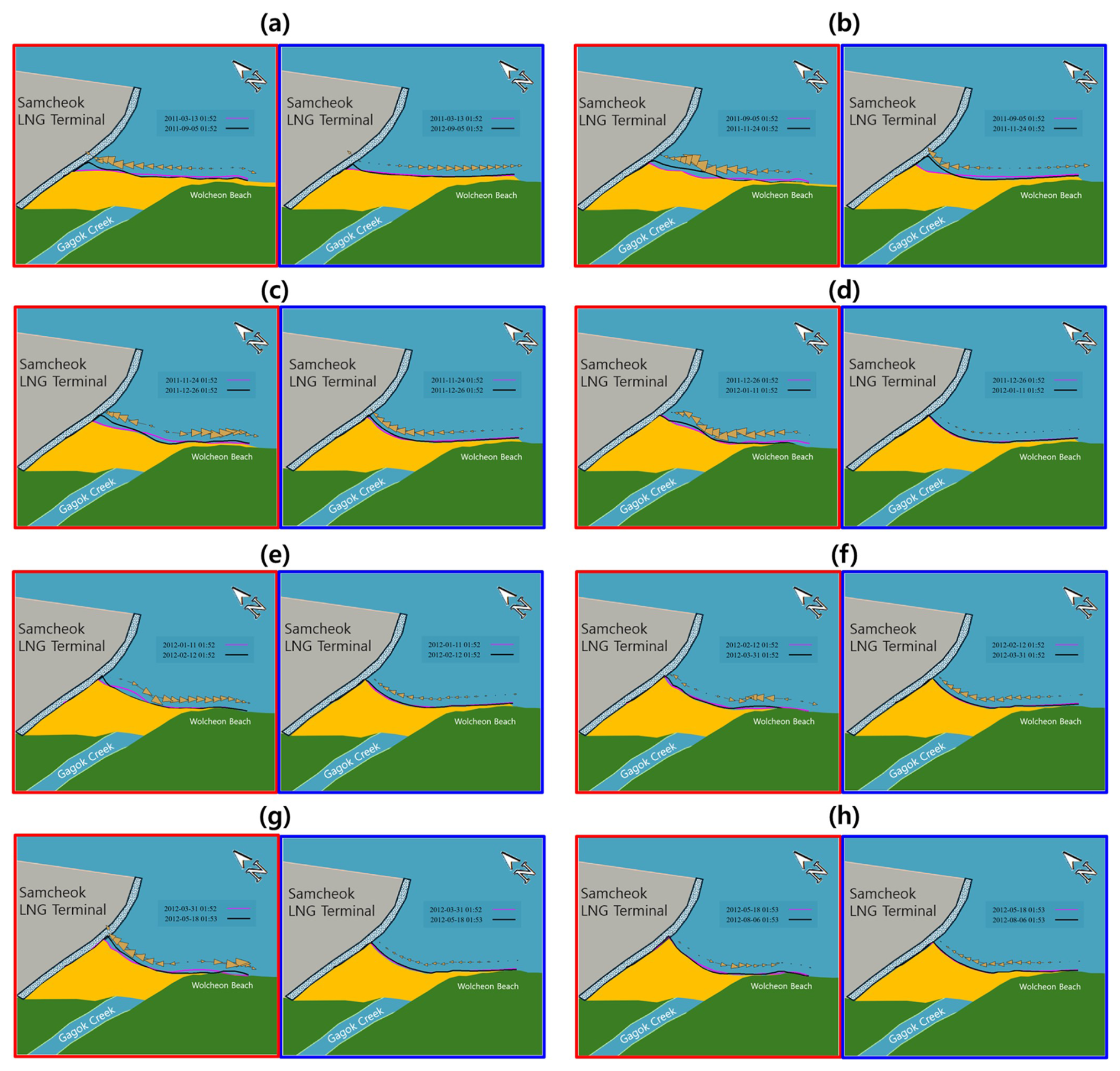
Figure 16 Comparison between LST vectors obtained from satellite images (left; red boxes) and numerically simulated LST vectors (right; blue boxes): (a) 13 March 2011–5 September 2011, (b) 5 September–24 November 2011, (c) 24 November–26 December 2011, (d) 26 December 2011–11 January 2012, (e) 11 January–12 February 2012, (f) 12 February–31 March 2012, (g) 31 March–18 May 2012, and (h) 18 May–6 August 2012.

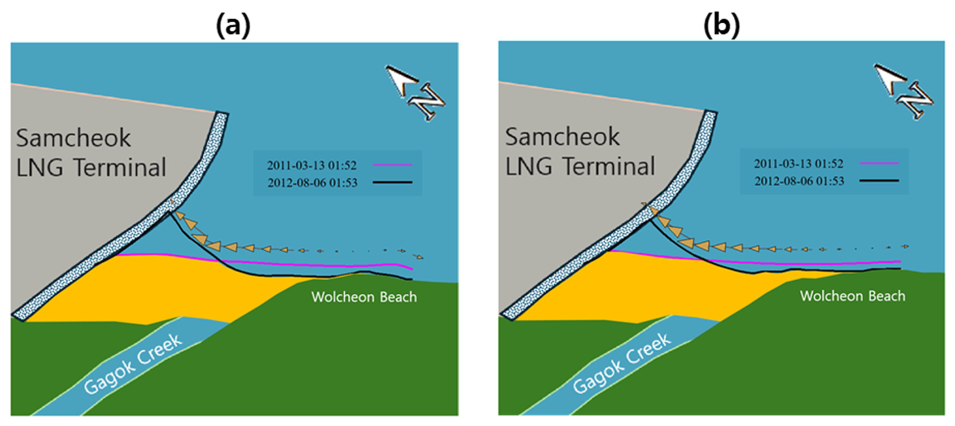
Figure 17 Comparison of LST vector results over the entire analysis period: (a) from satellite images and (b) from the shoreline change model.

Figure 18 compares the average magnitude of the LST vectors for each grid and the cumulative amount of long-shore sediment directed towards the LNG revetment, wherein a positive number represents the LST towards the LNG revetment and a negative number indicates the LST towards the opposite direction to the LNG revetment. Landsat 7 has a 30 m resolution, which allowed for the errors in the monitoring results presented in this study. Therefore, unlike the numerical results, the LST extracted from the satellite images in Fig. 18 included negative values. Analysis of the satellite images showed severe undulation compared to the numerically simulated results; therefore, the results obtained by smoothing through the front and back values, as expressed in Eq. (10), are shown together with the dotted line in Fig. 18. As a result, Fig. 18 shows that the smoothed results exhibit a fairly similar trend to the numerically simulated results.

$$\begin{array}{}\text{(10)}& {\stackrel{\mathrm{‾}}{Q}}_{\mathrm{ls},n}={\displaystyle \frac{\left({\stackrel{\mathrm{‾}}{Q}}_{\mathrm{l},n+\mathrm{1}}+{\stackrel{\mathrm{‾}}{Q}}_{\mathrm{l},n}+{\stackrel{\mathrm{‾}}{Q}}_{\mathrm{l},n-\mathrm{1}}\right)}{\mathrm{3}}},\end{array}$$

where Q_ls is the smoothed value of averaged LST and the subscripts n+1 and n−1 imply the value immediately following and before the ${\stackrel{\mathrm{‾}}{Q}}_{\mathrm{l}}$ value of the nth time, respectively.

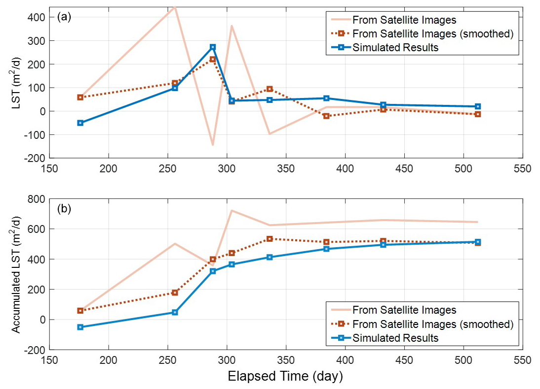
Figure 18 Comparison between LST magnitudes obtained from satellite images and numerically simulated LST (a) and cumulative amount of long-shore sediment towards the LNG revetment (b).

6 Discussion

6.1 Limitations

This study shows that the erosion damage caused by the Samcheok LNG terminal was due to excessive littoral drift resulting from wave deformation. In other words, the wave-induced nearshore circulation caused by the Samcheok LNG terminal triggered littoral drift, resulting in severe erosion. Additionally, numerical results were derived under average breaking-wave conditions based on the fact that the annual mean values from the NOAA dataset near Samcheok remained almost constant. The analysis, compared to Landsat 7 satellite images, yielded satisfactory results by comparing the accumulated LST. Although satisfactory results were obtained, the study had limitations owing to the assumptions made regarding the significant variables influencing littoral drift, such as a constant wave climate, sediment properties, and the LST coefficient.

This study suggests that a preventive strategy proposed at the planning stage is crucial for managing beach erosion downdrift in a harbor following a large coastal project. In addition, a preventive strategy that uses groins to control erosion can be found in Hsu et al. (2000), who reported examples from Japan in the 1970s–1980s. However, it should not be overlooked that beaches respond immediately to changes in the wave climate. Lim et al. (2021) reported that beaches respond not only to littoral drift but also to various factors such as sediment budget and cross-shore sediment transport. Furthermore, recent studies have highlighted that sea-level rise due to climate change has become a major consideration. Therefore, additional analyses are required for beaches that are exposed to erosion other than littoral drift.

6.2 Numerical analysis for mitigation strategies – groin placement

Large-scale coastal development near shorelines can cause significant topographical changes in adjacent coastal areas. In many cases, economic priorities take precedence, making it impossible to halt development, even in coastal areas with high conservation values. Therefore, we propose a solution using a hard engineering method that, despite its drawbacks, is the most direct and effective approach for preventing critical topographical changes and sand loss. Furthermore, in hard engineering, beach nourishment is unnecessary, as the sand that requires preservation is already present. Among the various functions of coastal structures, a groin is suggested as a means to mitigate sand loss caused by littoral drift.

The shoreline change predictions from the numerical model employed in this study suggested that littoral drift tended to move towards a large-scale structure, a trend that closely corresponded to the patterns observed in satellite imagery. Therefore, as mentioned previously, construction of a groin, which is a structure designed to reduce or block excessive sand movement, can serve as an appropriate mitigation measure. As a preliminary approach to erosion mitigation, a numerical model that incorporates littoral drift based on site-specific waves and coastal conditions may offer a more practical and reliable solution. Accordingly, the numerical model described in the previous section was applied to simulate and assess the impact of constructing one to three groins near the Samcheok LNG terminal. The input parameters related to the wave and coastal environments employed in this simulation were consistent with those presented in Table 1.

Because groin construction in an estuary is not feasible, this was excluded from consideration. Additionally, to enhance the practical applicability of the study, groins were assumed to be constructed along the southern beach where erosion damage had already occurred and were assumed to be sufficiently long to completely block littoral drift. Figure 19 illustrates the simulation results of the shoreline changes induced by construction of a group of groins. The results indicated that shoreline erosion decreased with an increasing number of groins, in contrast to the complete sand loss observed on the southern beach in the absence of groins. Although the results indicated that increasing the number of groins can more effectively inhibit sand transport, a comprehensive evaluation of cost-effectiveness and environmental impact is necessary to ensure that the desired beach width is achieved in a sustainable and efficient manner. Cost-effectiveness and environmental impact are regarded as separate and complex topics that are beyond the scope of this study.

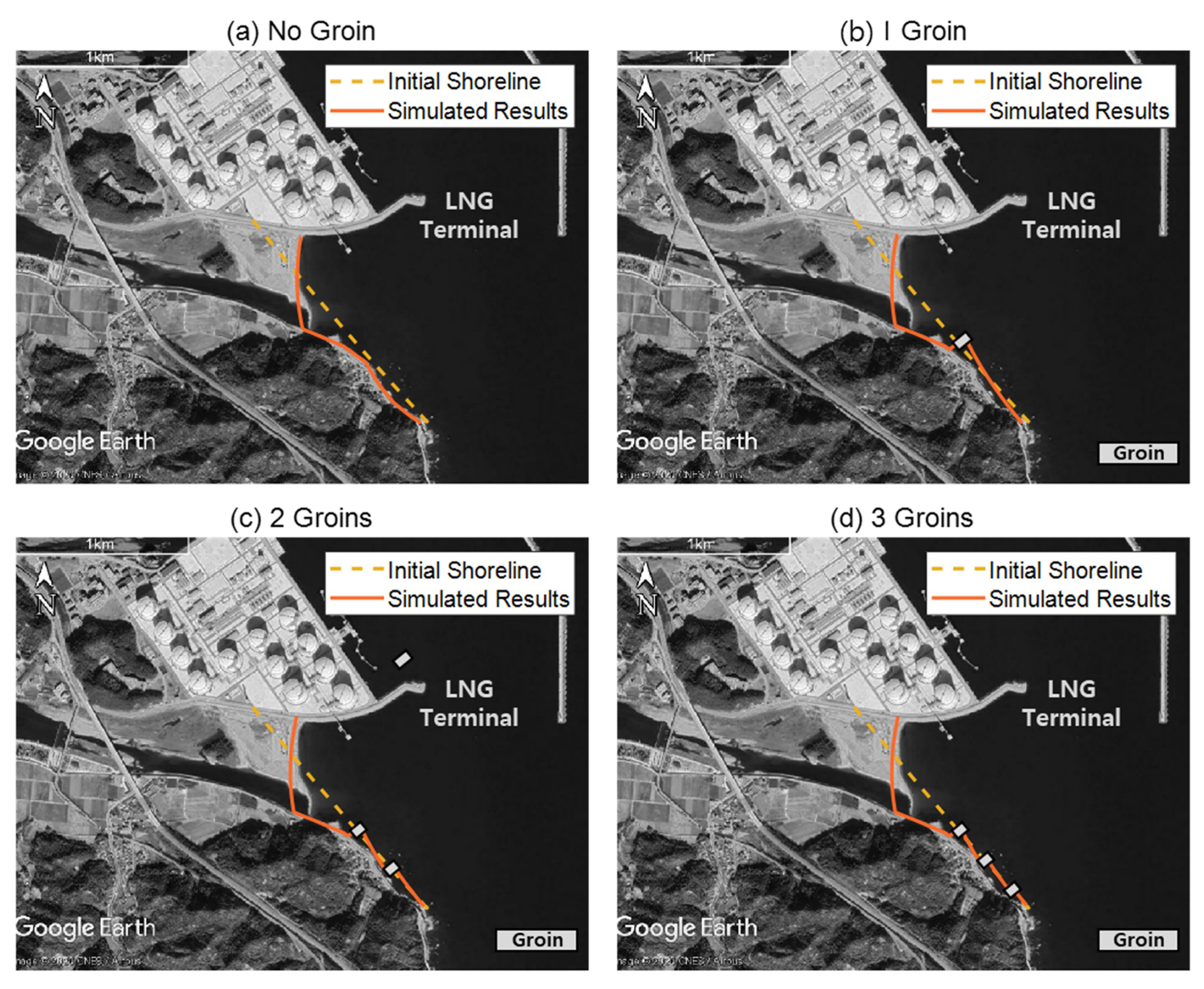
Figure 19 Simulated shoreline changes based on the number of groins constructed (© Google Earth): (a) no groin, (b) one groin, (c) two groins, and (d) three groins.

6.3 Theoretical analysis for mitigation strategies – groin placement

When the reclamation project was planned, action was not taken because of the absence of means to predict large-scale erosion in advance. Therefore, this section discusses appropriate measures that can be taken after assessing the impact of the construction of LNG revetments on the shoreline rotation and scale of LST by applying the PBSE, which predicts equilibrium shorelines. If LST occurs due to a change in the wave field, groins can serve as representative coastal structures for LST control (Hsu et al., 1993, 2000). Therefore, the potential effect of groin installation before performing the LNG project to prevent sand loss on Wolcheon Beach was examined. In addition, because a large shoreline rotation occurs, as identified in the equilibrium shoreline prediction, and installation of a single groin cannot achieve satisfactory performance, the effect of installing a group of groins was examined. Construction of the LNG revetment caused shoreline rotation at each point on Wolcheon Beach. To obtain the rotation angle (α_e) that ultimately converges, Eq. (4) (Sect. 4.2) was applied.

In the PBSE equation, it was assumed that the focus was located at the end of the LNG revetment (Fig. 11) and that the control point was located on the original shoreline of each θ grid cell. The rotation angle, α_e, provides the information required to approximately calculate the protrusion length of the groin to prevent sand loss from the beach with a beach width of W and a length of L_B (Fig. 20). In this calculation, the shoreline position in the groin is slightly lower than the seaward end point of the groin; however, it was assumed to be located at the groin end (Fig. 21). Figure 21 also shows the rotation angle α_e obtained from the Wolcheon Beach area located to the southeast of the Gagok Creek estuary under these conditions and the groin interval that is calculated accordingly.

Figure 20 Rotation of the equilibrium shoreline (a) and the beach preservation concept by groin installation (b).

Figure 21 Shoreline rotation angle results according to the θ grid cell (a) and the groin interval to prevent the sand loss by LST (b).

The original sand could not be maintained without the protrusion length because groins are not installed. However, if groins were installed, it can be seen that the groin interval would have increased with the groin protrusion length. If sand loss due to LST is to be prevented by installing a single groin on the 400 m long Wolcheon Beach, this can be achieved by installing a groin with a value of y_g=70 m, which shows a groin interval of approximately 400 m at x=700 m and x=600 m. If two groins with the same protrusion length are installed, y_g=30 m, which indicates that a first groin interval of 150 m and a second groin interval of approximately 250 m may be available. Therefore, the groin can be installed at x=600 m and x=750 m. Similarly, if three groins are installed, y_g=20 m shows that a first groin interval of 75 m, a second groin interval of 125 m, and a third groin interval of 200 m may be available. In this case, three groins can be installed at x=600 m, x=675 m, and x=800 m, respectively. These results indicate that a single groin is highly likely to cause problems because of the excessively large protrusion length of the Samcheok LNG terminal. Two groins are acceptable; however, it is desirable to install three groins with a protrusion length of y_g=20 m. The above calculations do not guarantee sand retention on the coast that exceeds x=1000 m, which is considered outside the Wolcheon Beach area.

7 Conclusions

In this study, a shoreline change model was applied to the complete loss of sand on Wolcheon Beach owing to the strong LST caused by a reclamation project for construction of the nearby Samcheok LNG terminal in Gangwon Province. The numerical model is applied to analyze severe beach erosion at the study site. The model can reflect the diffraction waves caused by coastal structures by applying the PBSE of Hsu and Evans (1989), unlike the conventional shoreline change model (Pelnard-Considère, 1957; Hanson, 1989).

The model results are verified using shorelines extracted from satellite images. Both the LST rate results obtained from satellite images and those obtained from the model confirmed that the sand on Wolcheon Beach moved to the Gagok Creek estuary on the largest scale during the winter season from 2011–2012. As a result of comparison with satellite images, the numerical model results reproduce the phenomenon of LST generation towards the LNG revetment owing to the LNG terminal reclamation project.

Although abundant knowledge of shoreline changes at the downdrift of harbors in Japan has been available since the early 1990s (Uda, 2010), there remains no up-to-date understanding of this type of beach erosion problem where the shoreline transitions from straight to embayed. When the reclamation project at the Samcheok LNG terminal was planned approximately 10 years ago, there was no adequate means to predict large-scale erosion in advance, whereas, if numerical predictions such as those in this study has been performed, effective countermeasures would have been possible. Among the causes of erosion, the main one is generation of LST due to large-scale reclamation; therefore, installing groins in advance is the most effective means to reduce erosion (Hsu et al., 1993, 2000; Uda, 2010). Applying PBSE, a well-known formula for predicting the rotation of the equilibrium shoreline owing to changes in the wave field, the effects of groin protrusion length and installation spacing on LST control and consequent sand conservation are investigated.

The results of this study showed that if a numerical model that predicts the shoreline change of a parabolic bay shape by approximately including wave diffraction effects is incorporated into the decision-making process for coastal disasters prior to large-scale construction in coastal areas, large-scale erosion problems, such as the case of Wolcheon Beach, can be avoided.