Hail events in Germany: rare or frequent natural hazards?

Hail represents a natural hazard in Germany and has potentially substantial economic and environmental impacts, but it often receives less attention than other weather phenomena. This, combined with the very local nature of hail, results in a lack of observations and further analysis. This study investigates hail characteristics across Germany using crowdsourced observations since 2000 and weather radar data from a 6-year period. A study using 3D printed hailstones provided insights into human perception of hail sizes, revealing that collective crowd estimates closely approximate actual measurements, though individual estimations can vary significantly. By deriving hail proxies out of radar data we analyzed hail frequency, spatial distribution and size variations. Our research reveals a gradient in hail occurrence, with southern Germany experiencing substantially higher hail probabilities compared to northern regions. Mountainous areas demonstrated increased hail frequency relative to lower-elevation territories. June emerged as the peak month for hail events, characterized by both highest frequency and largest hail sizes. This research contributes to a better understanding of hail as a natural hazard in Germany, providing valuable insights for risk assessment, insurance purposes and public awareness.

1 Introduction

Hail is a major natural hazard that causes severe damage with associated high costs. Although hail is not the natural hazard with the highest damage potential in Germany, it can lead to severe loss. Examples of very heavy, damaging hailstorms in Germany include the following: in July 1984, a hailstorm in Bavaria resulted in insured damages of EUR 1.5 billion; in July 2013 in Baden-Wuerttemberg an event led to EUR 3.6 billion damage; and the most recent large hailstorm in June 2023 led to a EUR 740 million total loss (DKKV, 2021; GDV, 2023). In an agriculture setting, hail has the greatest impact during the growing season, though the actual damage depends on many factors such as hail size, crop type and growth condition (Sánchez et al., 1996). Further hail damage can be expected to the infrastructure.

Measuring and observing hail is a difficult task. There are different sources of hail observations: human observations, indirectly through damages reported to the insurance companies, remote sensing, disdrometers and hailpads. Each of them has its own advantages and disadvantages. Human observations will always have the disadvantage of the spatial resolution. Most hail reports are made by people living in populous areas. Rural areas are very likely to be underrepresented. Thus, there is a reporting bias toward hail in cities and along roads (Allen and Tippett, 2015; McGovern et al., 2022). Furthermore, untrained reporters may have problems estimating the size of hail (we further investigate this in Sect. 4.2). The last problem occurs in every method of measuring hail: it melts when falling and while lying on the ground. This is one of the reasons why the exact size of a hailstone is hard to measure. It could also have an irregular shape, making sizing even more difficult.

Some aspects of human observations are also true for insurance data. Such data have a population bias and even a rich–poor bias, as the loss expense depends on the amount of insured property. The number of insured properties must also be accounted for. Another problem is the question of which hailstorms cause damage. Hohl et al. (2002) showed that the season must be included, as the high season produces fewer, but larger hailstones for the same kinetic energy than the low season. This is relevant for the mean damage, but has no noticeable influence on the total loss. Brown et al. (2015) highlight the need for diverse data that includes more than just weather, as the roof system is responsible for the most significant impact, accounting for 90 % of the total damage and this depends heavily on the material used and the condition of the roofing system. The largest damages nevertheless do not correlate with the maximum hail size (Ackermann et al., 2023).

To overcome the issue of population bias, weather radars can be a useful tool. They cover a large area and provide three dimensional (3D) data with high spatiotemporal resolution. We cannot derive hail size from radar data directly. Therefore, the challenge is finding a measure that is used as a proxy for hail and hail size. A first approach with single-polarized radars uses the reflectivity in combination with heights of specific temperatures which are derived from model data. Early on in hail research, Waldvogel et al. (1979) did a large study with hailpads to find a criterion for hail. They used the height of 45 dBZ (H₄₅) and the melting layer H₀. The hail probability at the ground should hereby be proportional to the difference of heights. With this approach, the probability of hail (POH) is calculated with a stepwise function using the difference between H₄₅ and H₀, whereby POH gets larger with increasing difference (Holleman et al., 2000; Witt et al., 1998; Nisi et al., 2016). The stepwise function was then adapted to a curve by Foote et al. (2005) and used, for example, in Trefalt et al. (2022).

Another method to estimate the hail size is the maximum estimated size of hail (MEHS/MESH) (Witt et al., 1998). MESH is based on the severe hail index (SHI), which takes the vertical integrated kinetic energy above the melting layer into account. The SHI is fitted to observed data to come up with a formula to obtain the maximum hail size (Witt et al., 1998; Murillo and Homeyer, 2019). MESH was originally developed for S-band radars in the US. Brook et al. (2024) showed that MESH used with C-band radars tends to overestimate hail sizes compared to S-band radars. To overcome this issue, Brook et al. (2024) introduced an empirical correction based on the matching of S-band and C-band radars in overlapping regions. Forcadell et al. (2024) utilize convolutional neural networks (CNNs) to obtain MESH values due to threshold-based optimization. In this study, we undertook our own calibration of the MESH formula with hail reports compared to the SHI derived from German C-band radar values (Sect. 4.5).

The upgrade from single- to dual-polarized radar systems gives the opportunity to improve the estimation of hail size. Aydin et al. (1986) and Depue et al. (2007) suggest the hail differential reflectivity H_DR, which combines the reflectivity Z and the differential reflectivity Z_DR. Ryzhkov et al. (2013), however, remark that the melting process of hail is neglected and propose a fuzzy-logic scheme that also includes the cross correlation ρ_hv, which is a measure of the uniformity of hydrometeors within a measured volume; large hail is expected to have lower ρ_hv values (Heinselman and Ryzhkov, 2006).

At Deutscher Wetterdienst, vertically integrated ice (VII) has been utilized operationally for years in the context of detecting potential hail occurrences. Its value to hail size relationship was developed by forecasters. It is important to note that VII is not widely recognized for its capabilities in hail size estimation. Wallace et al. (2019) used VII as a proxy for hail presence in the cloud in the US. The lack of use of VII serves as a motivation for the present study.

A different approach tries to estimate updrafts. For the development of the potential of large hailstones it is necessary to have strong updrafts, and Z_DR columns are used to estimate the presence and height of super-cooled water and can provide information on the location and strength of updrafts (Snyder et al., 2015). Another hint about updraft dimensions and the potential of large hail generation is the specific differential phase (K_DP) column (Snyder et al., 2017).

Puskeiler et al. (2016) and Puskeiler (2014) analyzed hail in Germany based on radar data with the cell tracking TRACE3D (Handwerker, 2002). Their hail climatology for Germany shows hotspots that are strongly linked to the orography. Junghänel et al. (2016) combined reported data with reflectivity values of radar data, either having a report and a reflectivity value higher than 50 dBZ or having a reflectivity value higher than 55 dBZ only. Similar results, also based on radar data, were found by Fluck et al. (2021). All the hail studies for Germany have a hotspot for hail in southern Baden-Wuerttemberg in common. Furthermore, they share a north–south increase of hail days. This was also observed in model-derived hail days (Battaglioli et al., 2023).

In this paper we derive multi-annual hail data (2018–2023) for Germany based on VII. We compare it to crowdsourced data and investigate the annual cycles and spatiotemporal frequencies. In a case study we depict the similarities and differences for different hail size estimation methods. We focus on two research questions.

• Can we rely on the size estimation in human-observed hail data?

• Are the radar based algorithms VII and MESH suitable for determining hail (size) climatologies for Germany?

2 Data

2.1 Human observed data

There are three different sources for human observed data in Germany: the WarnWetter app, the European Severe Weather Database and staffed weather stations.

The first source are user reports obtained from the WarnWetter app. This mobile phone application operated by Deutscher Wetterdienst (DWD) informs the public about current and forecast weather and provides weather warnings. The application enables users to submit reports on their observations of weather conditions as well as upload pictures. Upon reception, all user reports are quality checked with reference data, e.g., radar data (Spitzer et al., 2023). Regarding hail, users can select between the following options: Hagel unter 1 cm, Hagel 1 cm, Hagel 2 cm, Hagel 3 cm, Hagel 5 cm, Hagel größer 7 cm (hail under 1 cm, hail 1 cm, hail 2 cm, hail 3 cm, hail 5 cm, hail above 7 cm). The already quality-checked reports are cleaned up for further analysis, so users who reported an event for a day no other user reported an event are excluded, and for users who reported more than one event in 30 min, only the report with the largest hail size is taken into account.

The European Severe Weather Database (ESWD) (Dotzek et al., 2009) was established in 2006. It contains data contributed by the public (eyewitnesses and voluntary spotters) on severe convective storm events and is quality controlled. With an update in the year 2008 the quality control was further enhanced. It contains four steps, from basic plausibility checks to fully verified (Dotzek et al., 2009). In this analysis we use data with basic plausibility checks (QC0+). The first reports are available for 2000 even though the test phase of the ESWD started in 2004. A severe hail event is characterized by a maximum hail diameter larger than 2 cm. From 2021 on, some of the reports of the WarnWetter app are transferred to the ESWD. There is a continuous increase in reports from 2000 until 2008 with a maximum of approximately 300 reports in a year. Compared to the previous years, in which there was no major change, there was a drop of reports in the years 2014–2018 (160–200 reports per year).

The largest dataset comes from station observations of the monitoring network operated by DWD. It combines staffed weather stations and trained volunteer reports. The temporal accuracy of those reports differs from daily reports up to the exact time of the hail event. In order to combine them, only the reported day of occurrence is taken into account. Due to the continuous automation of weather observations, the number of reports decreases with time. For this reason the dataset only contains data up to 2017.

The problem of point observation data is the low and irregular spatial resolution. Rural areas might be underrepresented due to the lack of people who can report an event. Thus, the crowdsourcing data can only provide information about positive events, as no report does not automatically mean no hail. The station observations, however, can also give a hint about the absence of hail.

All in all, there are 3769 hail reports in the ESWD from 2000 to 2020. All reports independent of their quality level (QC0+ and higher) were used in our study. Furthermore, the reports of hail (since 2021) from the new DWD WarnWetter app were used. They are automatically checked for plausibility and partially included in the ESWD dataset, amounting to 39 142 reports. Inclusion in the ESWD involves a manual check of the content and plausibility of the reports for hail sizes greater than 2 cm. Hail sizes smaller than 2 cm are not included. To ensure no duplicates were included in our analysis, ESWD data from 2021 and newer was excluded. The smallest category “Hagel unter 1 cm” (hail smaller than 1 cm) was left out in the analysis due to the possibility to mistakenly reporting graupel instead of hail. With that, 21 231 reports remained in the analysis from the WarnWetter app. For the years 2000 to 2017, 25 719 reports of the station observations of the DWD are available. In total the analysis includes 50 719 hail reports.

2.2 Radar data

The German radar network consists of 17 C-band Doppler radars and covers the whole of Germany and adjacent areas (see Fig. 1). An upgrade from single- to dual-polarization radars was started in 2011 and finished in 2021. Each radar provides scans in 11 elevation angles every 5 min (see Fig. 2).

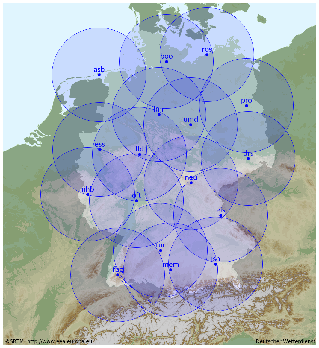
Figure 1 The German radar network with its 17 C-band radars.

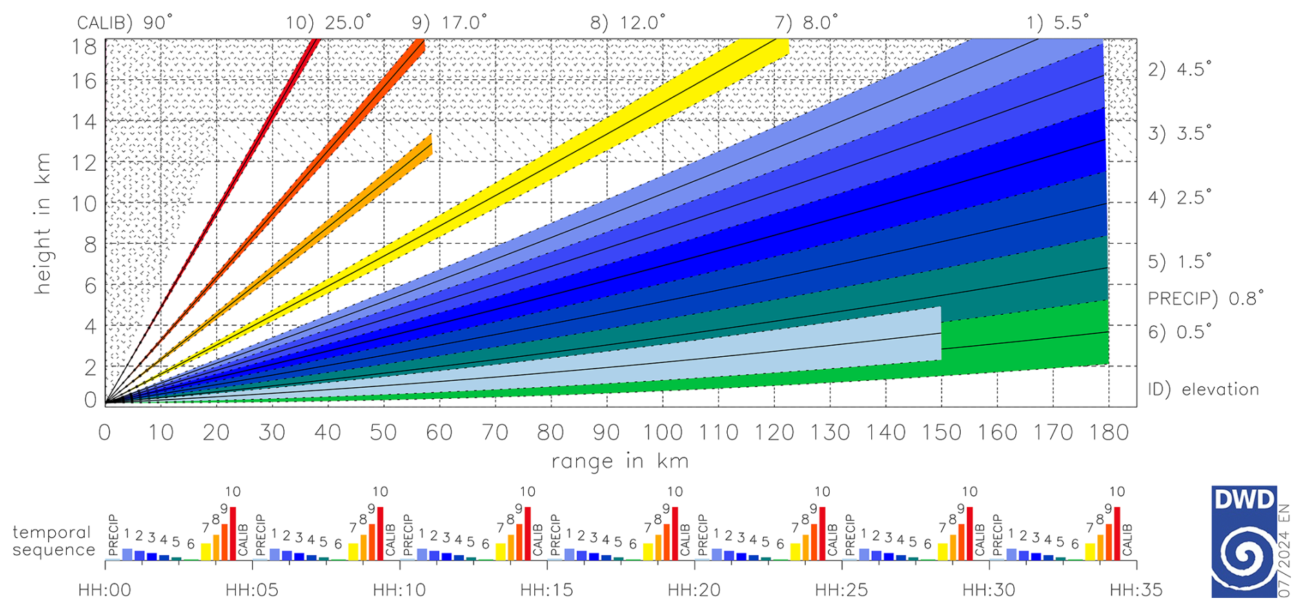
Figure 2 The DWD radar scan strategy since 2012 with its 10 volume scans and 1 precipitation scan.

The volume scan has a range of 180 km. The precipitation scan, a low-elevation scan that follows the orography, covers a range of 150 km. Both scan types have a horizontal resolution of 1° × 250 m.

In this study, we will evaluate the years 2018–2023, with a particular focus on the convective season between April and September.

2.3 Insurance data

The federation of private insurance companies in Germany, the German Insurance Association (GDV), has kindly provided access to their hail damage data, with hail and storm forming one category. The decision for defining an event into one of the “hail,” “storm” or “undefined” categories is unfortunately prone to errors. For this study we only included data with reports resulting in hail damage. For each date with hail damage information concerning the postal code, the damage expense, the number of damages, the insurance expense and the number of insurance contracts in each postal code is provided. From April to September in the years 2013 to 2022 there are 526 444 insurance claims for different postal codes and days of hail. In total, from 1830 possible days, 1815 (99.18 %) are recorded as having at least one occurrence of hail damage in Germany. This is because the damage cannot always be assigned to the precise day on which it occurred. The data is derived solely from postal code areas and therefore may not provide a complete picture of hail events. This limitation is why we chose to leave spatial analysis out of our examination of insurance data. By focusing primarily on larger hail events, we may inadvertently overlook occurrences of smaller hail, which are equally significant. So we focus on the temporal analysis of hail occurrences of insurance data.

3 Methods

This study focuses on two different radar-derived proxies to detect hail size: VII and MESH. The first step for both VII (Sect. 3.1) and MESH (Sect. 3.2) is to collect the 11 radar elevation scans that will be used to construct a 3D data cube of reflectivity measurements, a composite in three dimensions. The geometric height of different temperature levels is derived from vertical temperature profiles the ICON-D2 (Icosahedral Nonhydrostatic) model (Reinert et al., 2020) and combined with the 3D data cube.

For both algorithms, a minimum threshold of 7.5 mm is used to discriminate between hail and no hail.

3.1 Vertically integrated ice (VII)

VII is a measure of the frozen water content in a vertical column. At DWD it is expressed in water equivalent and, therefore, differs from the definition established in the literature (Gauthier et al., 2006; Mosier et al., 2011). The height of the temperature at −10 °C, H₋₁₀, is approximated by the height of the melting layer H₀ with a constant height offset. VII is calculated from the radar reflectivity Z by

$$\begin{array}{}\text{(1)}& \text{VII}=\underset{H_{-\mathrm{10}}}{\overset{H_{-\mathrm{\infty }}}{\int }}\mathrm{3.44}\times {\mathrm{10}}^{-\mathrm{6}}{Z}^{\frac{\mathrm{4}}{\mathrm{7}}}\mathrm{d}H\end{array}$$

During the internal evaluation process of the VII product, forecasters proposed a linear relationship between observed hail size and VII: VII_hailsize[mm] = VII ⋅ 0.75 (Böhme et al., 2017).

3.2 MESH

With the 3D data cube of reflectivities, it is possible to calculate the severe hail index (SHI). The SHI is calculated by transforming reflectivity data (Z) between Z_L = 40 dBZ and Z_U = 50 dBZ (W(Z)) into the hail kinetic energy flux ($\stackrel{.}{E}$), applying a temperature weighting function (W_T(H)), and vertically integrating this value from the storm top to the radar level (Witt et al., 1998). The heights for the melting layer (H₀) and for a temperature of −20 °C (H₋₂₀) are derived by ICON-D2.

$$\begin{array}{rl}& W\left(Z\right)=\left\{\begin{array}{ll}\mathrm{0}& \text{for}Z\le Z_{\mathrm{L}}\\ \frac{Z-Z_{\mathrm{L}}}{Z_{\mathrm{U}}-Z_{\mathrm{L}}}& \text{for}{Z}_{\mathrm{L}}<Z<Z_{\mathrm{U}}\\ \mathrm{1}& \text{for}Z\ge Z_{\mathrm{U}}\end{array}\right.\\ & \dot{E}=\mathrm{5}\times {\mathrm{10}}^{-\mathrm{6}}\times {\mathrm{10}}^{\mathrm{0.084}Z}W\left(Z\right)\\ & W_T\left(H\right)=\left\{\begin{array}{ll}\mathrm{0}& \text{for}H\le H_{\mathrm{0}}\\ \frac{H-H_{\mathrm{0}}}{H_{-\mathrm{20}}-H_{\mathrm{0}}}& \text{for}{H}_{\mathrm{0}}<H<H_{-\mathrm{20}}\\ \mathrm{1}& \text{for}H\ge H_{-\mathrm{20}}\end{array}\right.\\ & \text{SHI}=\mathrm{0.1}\underset{H_{\mathrm{0}}}{\overset{H_T}{\int }}{W}_T\left(H\right)\dot{E}\mathrm{d}H\end{array}$$

From that, we can deduce the MESH. MESH was first derived by Witt et al. (1998). They used 147 hail observations for their derivation of SHI to MESH. As the intention of MESH is to anticipate the maximum possible hail diameter, the resulting value should be higher than 75 % of the observations. This leads to

$$\begin{array}{}\text{(2)}& \text{MESH}\left[\mathrm{mm}\right]=\mathrm{2.54}\cdot {\text{SHI}}^{\mathrm{0.5}}\end{array}$$

Murillo and Homeyer (2019) revised the approach and used 5897 observations to fit the power law. The resulting new power laws, one with the MESH values higher than 75 % of the observations and one with them higher than 95 %.

$$\begin{array}{}\text{(3)}& {\displaystyle }\text{MESH}[\mathrm{mm}{]}_{\mathrm{75}}=\mathrm{15.096}\cdot {\text{SHI}}^{\mathrm{0.206}}\text{(4)}& {\displaystyle }\text{MESH}[\mathrm{mm}{]}_{\mathrm{95}}=\mathrm{22.157}\cdot {\text{SHI}}^{\mathrm{0.212}}\end{array}$$

Both fittings were made with S-band radars in the US. As we can make use of a great amount of observation data, we have derived our own SHI–MESH relationships for the German C-band radar network.

With the WarnWetter app we also have the opportunity to derive a power law for our region of interest. We must take into account that the observations made via the WarnWetter app are given in categories. Therefore, we have selected the reference values from the category (see Sect. 2.1). For example, a report from the category “hail of 2 cm” was assumed as an observation of a hailstone with a diameter of 2 cm although it might be slightly smaller or larger. For the category “under 1 cm” a value of 0.5 cm and for “above 7 cm” a value of 7 cm were defined as reference points. We took the highest SHI in a 5 km radius around the observation and in the last 15 min before the observation took place, as the report should be done after the hail reached the ground. Only data from April to September of the year 2022 and 2023 and SHI–observation pairs where the SHI was higher than 10 were used . Our fittings for the larger hail sizes may not be optimal due to the lack of data. We only had 36 observations for 7 cm, as they are prone to errors and varied a lot in their SHI values, so we left them out in the fitting. In total we had 2403 samples for 0.5 cm, 4232 samples for 1 cm, 1979 samples for 2 cm, 750 samples for 3 cm and 192 samples for 5 cm. From that we obtain the power laws out of 9556 observations:

$$\begin{array}{}\text{(5)}& {\displaystyle }\text{MESH}[\mathrm{mm}{]}_{\mathrm{75}}=\mathrm{0.4607}\cdot {\text{SHI}}^{\mathrm{0.8665}}\text{(6)}& {\displaystyle }\text{MESH}[\mathrm{mm}{]}_{\mathrm{95}}=\mathrm{0.9216}\cdot {\text{SHI}}^{\mathrm{0.9739}}\text{(7)}& {\displaystyle }\text{MESH}[\mathrm{mm}{]}_{\mathrm{mean}}=\mathrm{0.0071}\cdot {\text{SHI}}^{\mathrm{1.4877}}\end{array}$$

Figure 3 depicts the relations of SHI to reported hail sizes. It is important to note that the fitting to the power law is very sensitive.

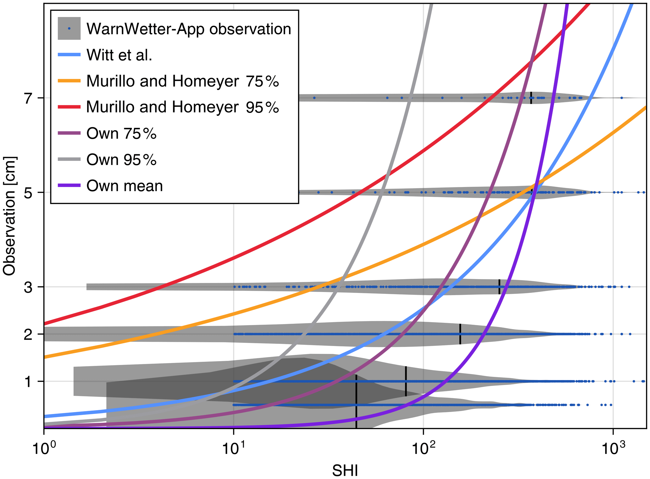
Figure 3 Comparison of all power laws of SHI (colored lines) to observation values (blue dots) in a violin plot visualizing the number of observations (shaded area) including the median SHI (black vertical bar) of the data from the German WarnWetter app for the years 2022 and 2023.

4 Results

In the following, we present the results for hail observations in Germany, focusing on three key areas. First, we examine the human observed data, highlighting its quality and characteristics. Next, we analyze hail sizes and occurrences as detected by C-band weather radars, comparing the findings of two different algorithms with human observed data to assess their quality. Finally, we explore the economic impact of hail events through insurance data and show how hail events can lead to significant financial losses in the region.

4.1 Human observed data

In this section, we examine various sources of human observed data. We first assess the quality of crowdsourced data through a survey. This study used 3D printed hailstones to evaluate how precisely people estimate the size of hail. With these finding as context, we then present spatial and temporal patterns of human observed data across Germany.

4.2 Assessing the quality of human observed data

To develop and improve algorithms that identify hail events from radar observations, validation data is required. However, it is unclear whether user reports from the WarnWetter app are reliable enough to provide additional information for validation purposes. To answer this question, we conducted a brief study using 3D printed hailstones based on hail models (Mirkovic and Zrnic, 2023) (see Fig. 4).

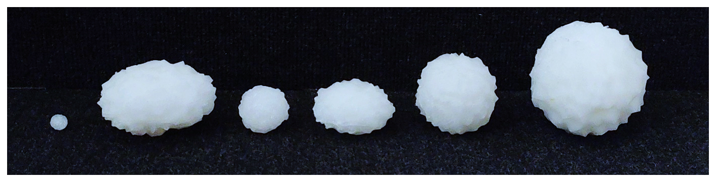
Figure 4 Six examples of 3D printed hailstones in different sizes and forms. From left to right: round 0.5 cm, oval 7 cm, round 2 cm, oval 5 cm, round 5 cm, round 7 cm.

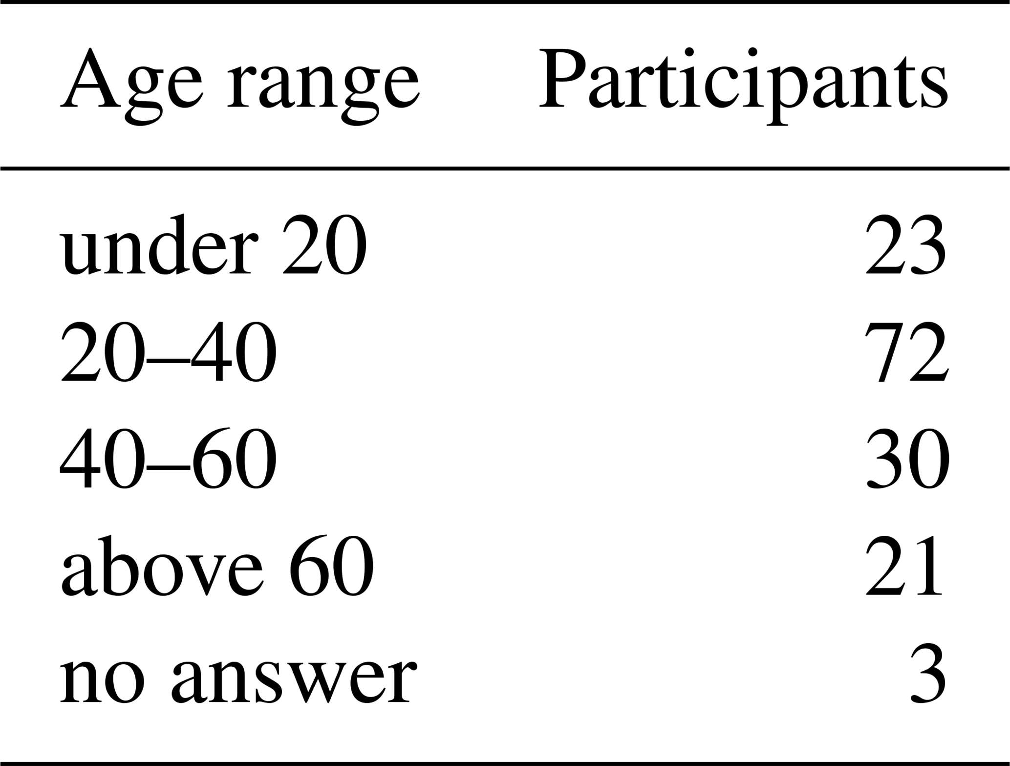
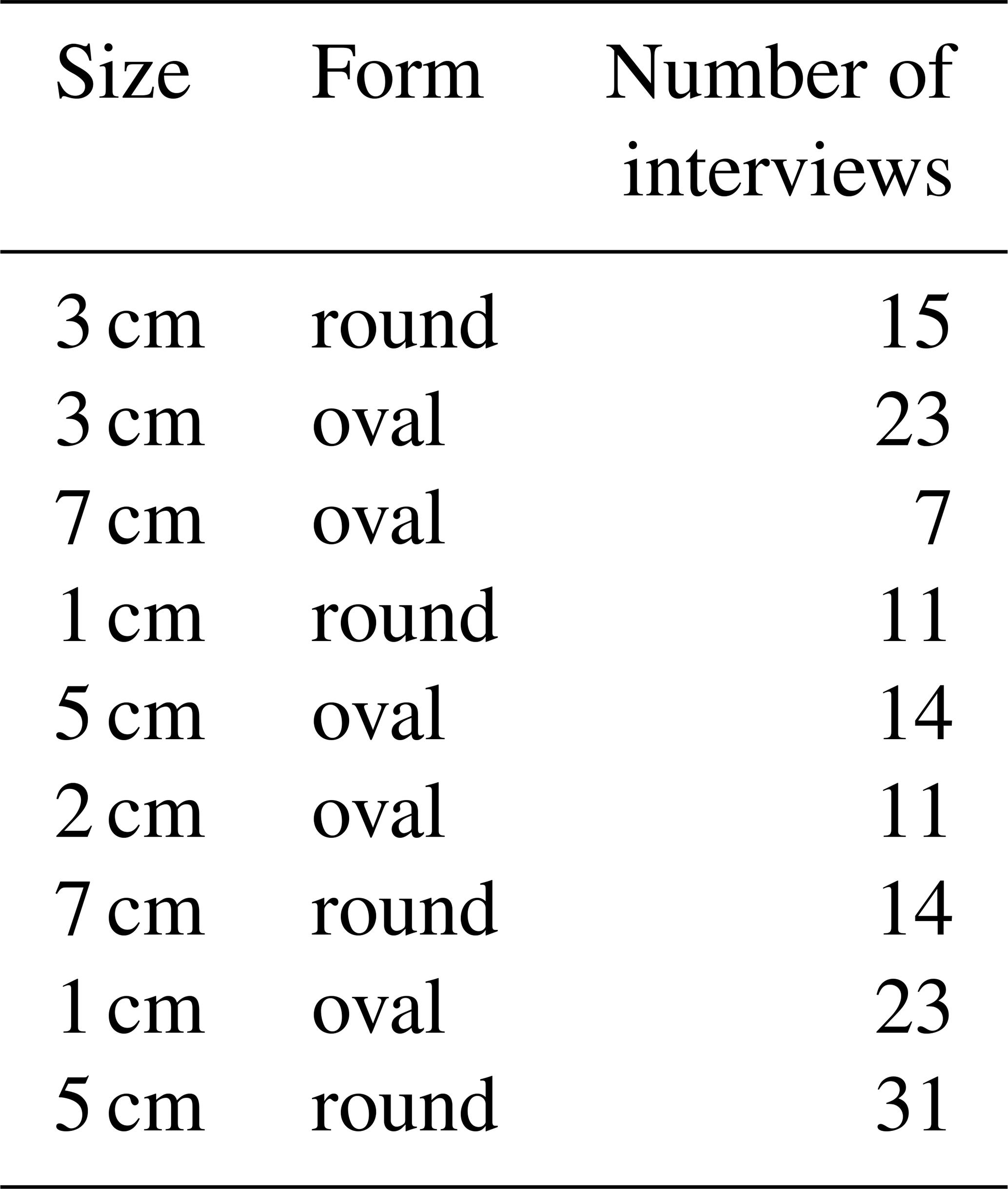
In total we had 12 hailstone samples in use, 6 round and 6 oval (diameter 2:1) with sizes of the maximum dimension of 0.5, 1, 2, 3, 5 and 7 cm. In the study we asked questions relating to nine of those hailstones. In total, we surveyed 149 participants (76 male, 68 female) with the age distribution as shown in Table 1. Table 2 lists the number of interviews for the different sizes and forms of the hailstones. After the participants accepted the data processing, they were asked to estimate the diameter of a EUR 2 coin to obtain a control value for their ability to estimate sizes, independently of a hailstone. Following this, they were asked to estimate the size of the presented hailstone. The survey included two separate values. In the first phase, participants were asked to answer freely. In the second phase, they were given options for their answers. The options were the same as in the reporting process of the WarnWetter app:

Table 1 The number of people surveyed in each age group, categorized by age.

Table 2 The number of interviews for each hailstone.

Hagelkorngröße (hail size)

• unter 1 cm (Linse) (under 1 cm lentil)

• 1 cm (Erbse) (1 cm pea)

• 2 cm (10 Cent Münze) (2 cm 10 cent coin)

• 3 cm (Kronkorken) (3 cm crown cork)

• 5 cm (Golfball) (5 cm golf ball)

• über 7 cm (Tennisball) (above 7 cm tennis ball)

In addition, demographic data was gathered for statistical evaluation.

The true value of the diameter of a EUR 2 coin is 2.575 cm. The estimated mean diameter of all survey participants is M = 2.538 cm, with a minimum of 1 cm and a maximum of 6 cm. We were interested in determining whether there is a discrepancy among age groups due to differing degrees of experience with the digital world or its attendant technologies. The distribution of answers for the different ranges of age can be found in Fig. 5. Most of the age groups underestimated the size of the coin; only the 20–40-year-olds overestimated the size in the mean, but in the median they were very good with 2.5 cm. The best mean was achieved by the group of under 20-year-olds with M = 2.508 cm, but both of these groups had some outliers with 5–6 cm and low medians.

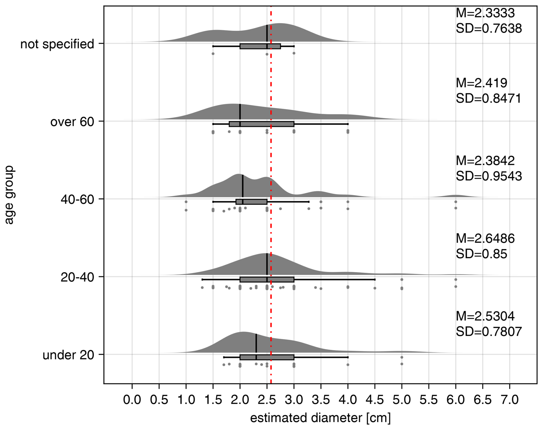
Figure 5 The distribution, with the median of each answer (black vertical bar), for the question “How large is a EUR 2 coin?” for the different age groups. The correct answer is shown as red dashed line. The mean and standard deviation for each group are presented on the right of each subplot. The answers are shown using three different visualizations for each subplot. Top: a kernel density estimation for all answers in the age group showing the distribution of answers; middle: a box plot showing the quartiles and outliers; bottom: the answers given as dots showing all single values.

As depicted in Fig. 6, when the categories were given as options, participants chose the right category most of the time (75.17 %). Additionally, when the wrong choice was made, most of the time a smaller category was chosen (18.79 %). There is no difference between the results for round and oval hailstones. Figure 6 also shows the free estimation of hail stone size in cm as a kernel density estimation. Without the option to choose a category, the distribution of answers is much broader, but still with a median that is close to the right size. The distributions are almost symmetrical, with a median which tends to be too small. The deviation to the true value stays similar through all sizes.

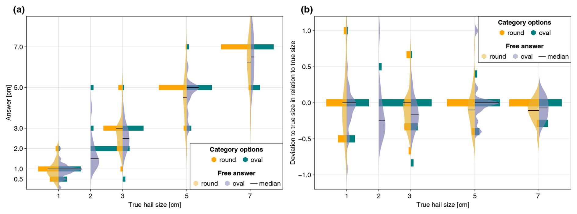
Figure 6 (a) The distribution of answers estimating the size of the presented hailstones as bars for the category options and as kernel density estimations, with each median, for the free answers. (b) The deviation from the true hail size in relation to the true hail size.

Finally, we compared the results of the initial estimation question about the size of the EUR 2 coin with the results of the freely given answers for the hailstones. Figure 7 clearly shows that there is no clear linear relationship between those two answers. This may be due to the fact that the hailstone was presented and could be touched. Most of the participants needed to imagine the size of a EUR 2 coin.

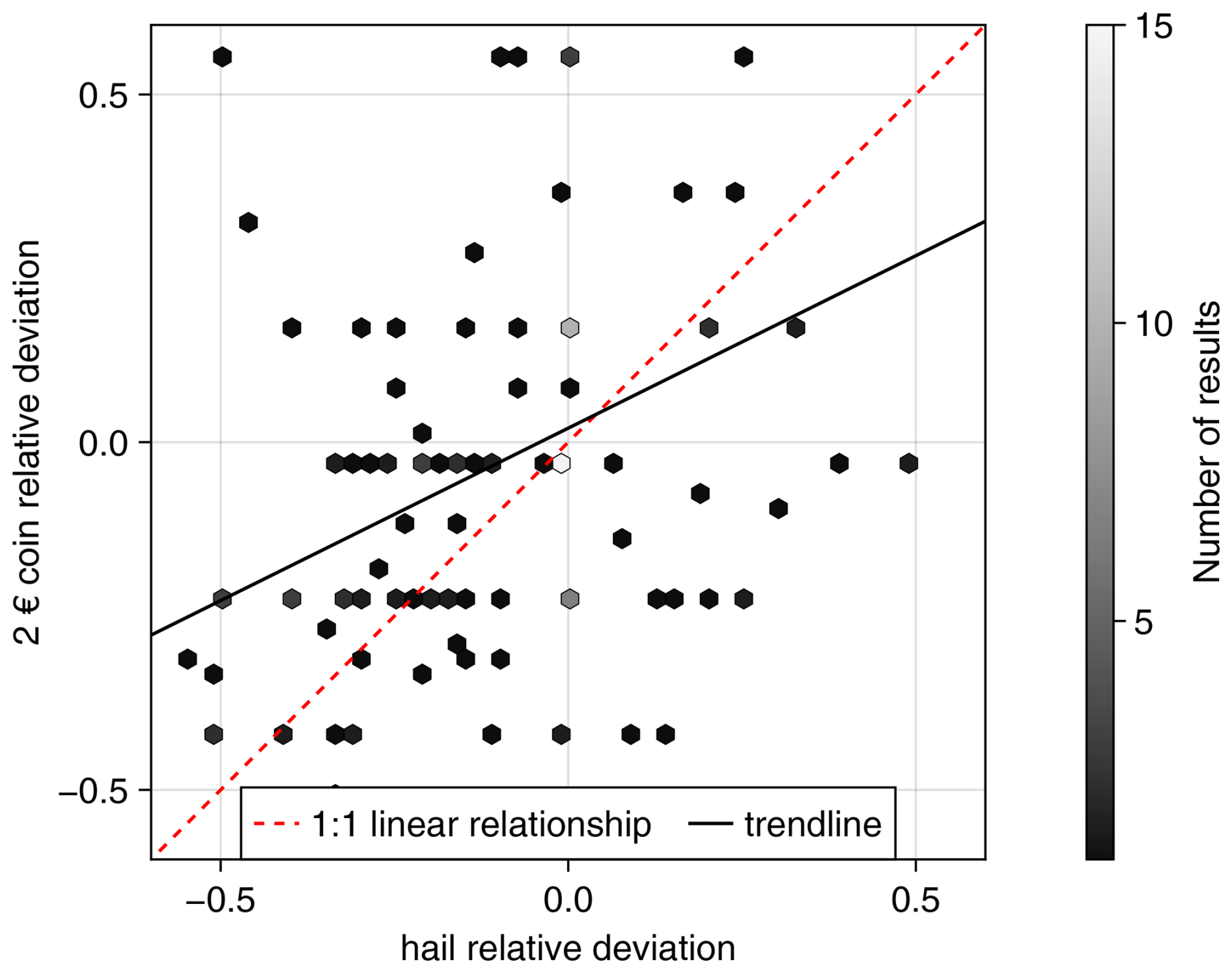
Figure 7 The comparison of deviations from the estimation of the size of a EUR 2 coin and the freely given answers to the hailstone size estimation.

In conclusion, we can say that the mean of the estimated sizes is quite good and close to the real value, but individual estimations can be quite inaccurate. It seems that estimating the size of an object of imagination, like the EUR 2 coin in our survey, is not directly comparable to an object that is visible. Most of the answers to the categorical options were right, but there are also some wrong answers. As we have a low spatial density of observations in the WarnWetter app most of the time, we need to keep in mind that there might be wrong values due to bad estimation abilities. If the estimation of the size is off, it is likely to be underestimated. The bias remains constant irrespective of hail size; however, the standard deviation undergoes a reduction for larger hail sizes. Giving the categories seemed useful, as the number of wrong categories is noticeable only for small hail sizes.

4.3 Analysis of crowdsourced data in Germany

Based on crowdsourced data from ESWD, the WarnWetter app and station observations we will address the questions of diurnal and annual cycles and hotspots of hail in Germany. In Fig. 8a the diurnal cycle of hail reports is depicted. For this analysis the station observations were excluded due to missing information concerning the time of the hail event.

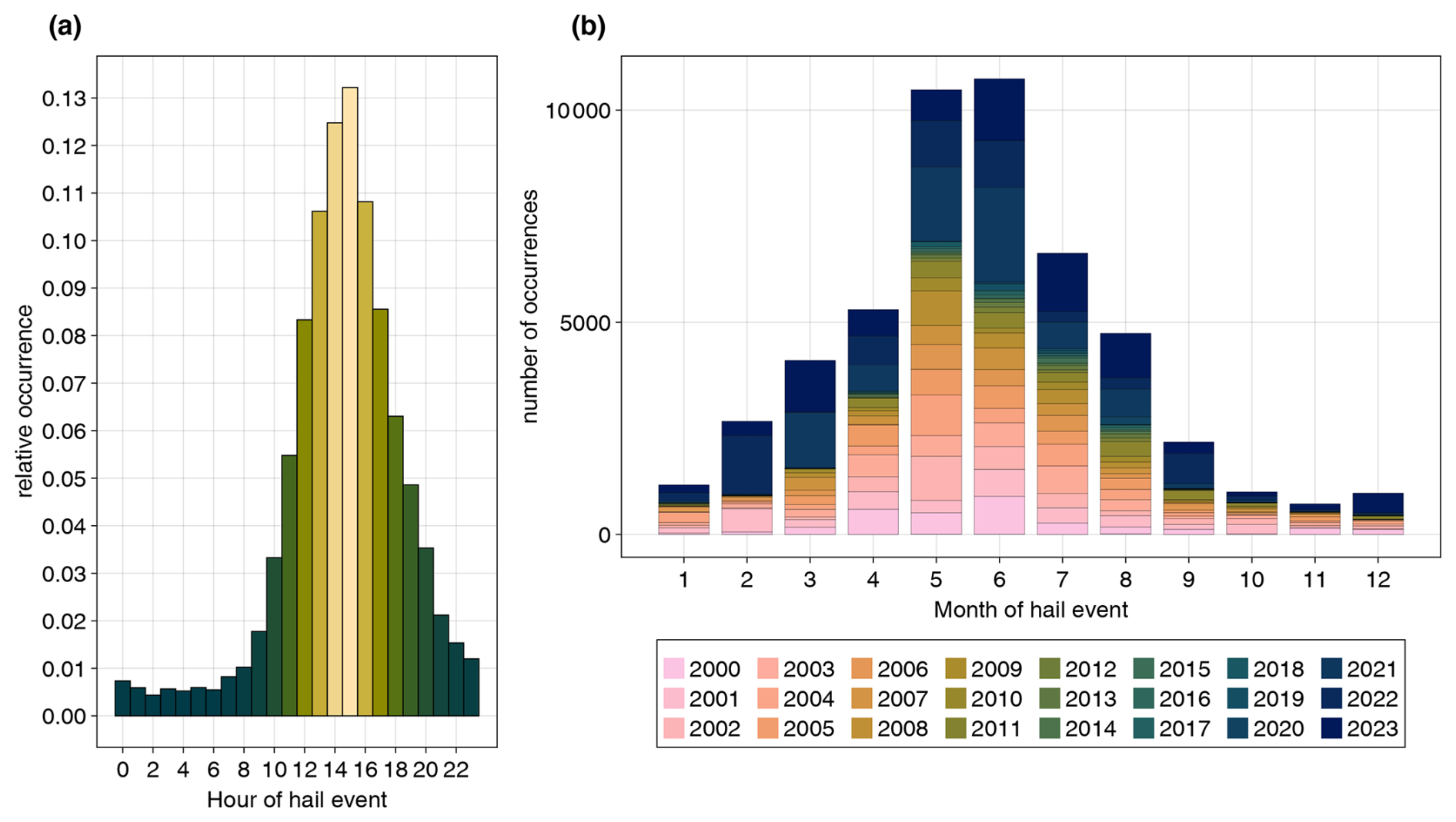
Figure 8 Hail observations in (a) the diurnal cycle based on data from ESWD (3769) and WarnWetter app (21 231) and (b) the annual cycle based on data from station observations (25 719), ESWD (3769) and WarnWetter app (21 231).

The number of hail observations clearly shows a diurnal cycle, as the reports are very close to a normal distribution around 15:00 UTC (17:00 CEST), with a standard deviation of about 3 h. Reports of night time (23:00–08:00 UTC, 01:00–10:00 CEST) hail events are rare. There are also two months in which there is a higher probability of hail being observed, namely May and June (see Fig. 8b). Beyond the convective season the number of reports is negligible with the exception of March 2021 and February 2022. In total, there are many more reports from the WarnWetter app than from the ESWD, as visible through the higher numbers since 2021. Figure 9 depicts the reported sizes in the ESWD and the WarnWetter app. Small hail occurs more prominently from February to September. Medium hail occurs mainly in June, but also in May, July and August. In Germany only a few reports of hail that exceeded 5 cm were recorded in the last 23 years. Large to giant hail is most likely to occur from May to August.

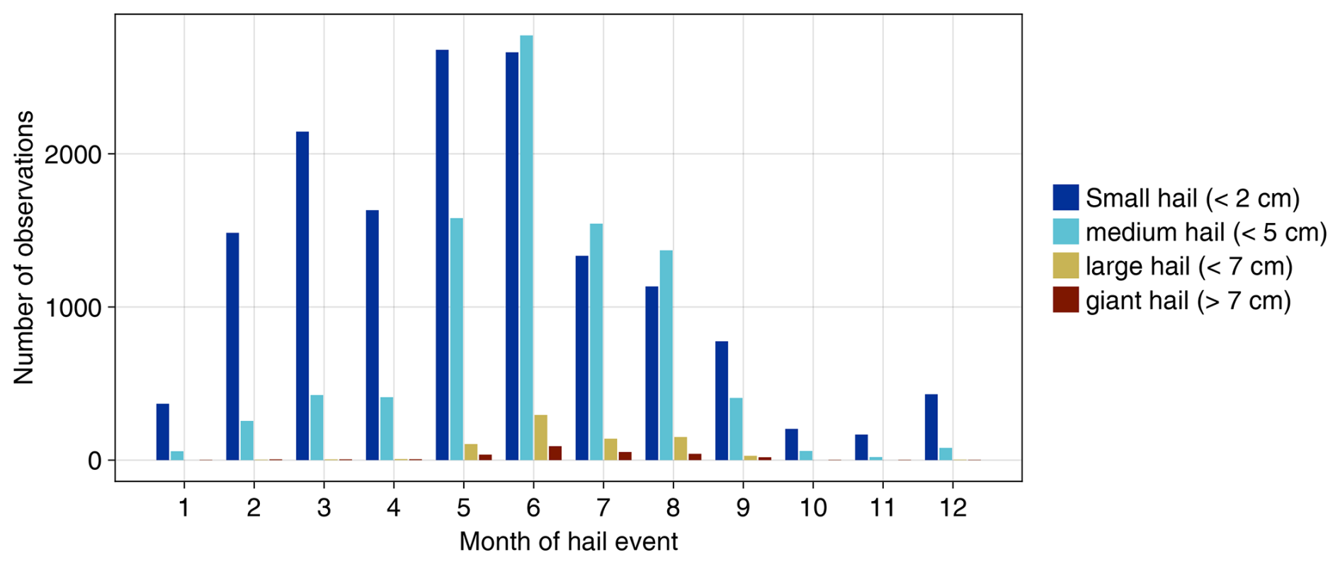
Figure 9 Distribution of observations of hail sizes in Germany from the ESWD and the WarnWetter app.

The distribution of hail reports in Germany is displayed in Fig. 10a in a h3 grid of level 6 (Uber Technologies Inc., 2018). There are some hotspots visible in the south of Bavaria (close to Munich), in the middle of Baden-Wuerttemberg (close to Stuttgart), in North Rhine-Westphalia in the Ruhr valley, Hessia in the Rhine-Main region and Berlin. In the north of Germany there are only a few hail reports. All areas with hail hotspots have a high population (see Fig. 10b). To examine whether the observations underlay an urban reporting bias, Fig. 10c shows the number of observations in a cell, normalized to the population. No such hotspots are now visible, and only the Pre-Alps have a slightly higher number of observations than the rest of Germany. Some cells are more noticeable because of station observations that have been in one place for a long time and therefore reported hail for each day if apparent. In conclusion, the absence of hotspots in the normalized Fig. 10c clearly emphasizes the existence of an urban reporting bias, as there is no longer a visible difference in hail occurrence over Germany.

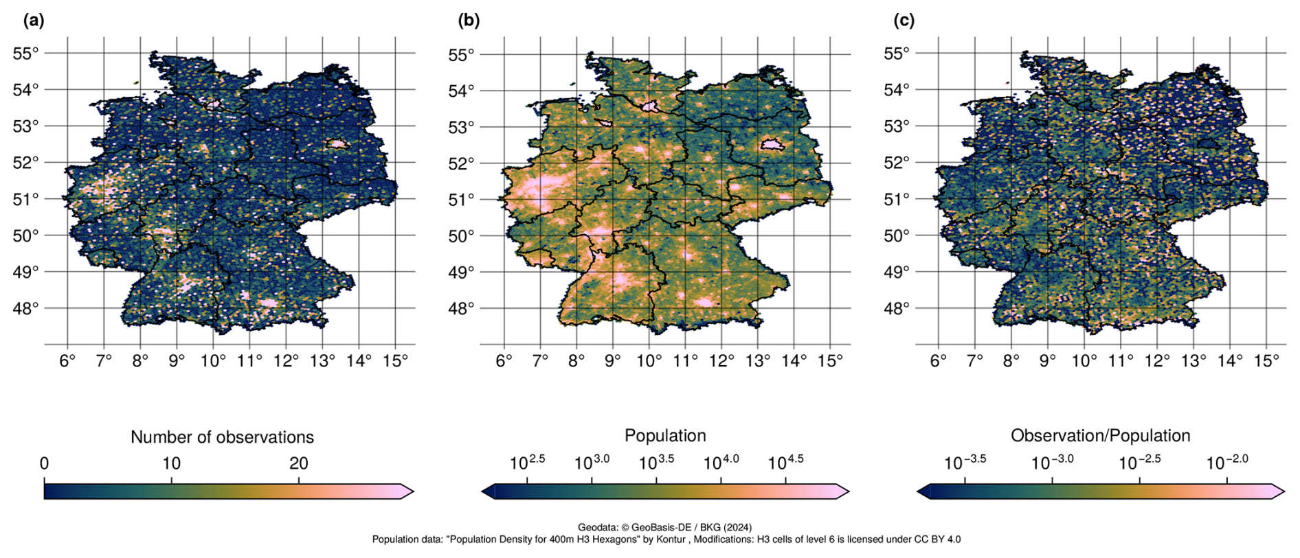
Figure 10 (a) Number of crowd observations in Germany 2001–2023 based on data from station observations, ESWD and the WarnWetter app. (b) Population in Germany. (c) Number of observations normalized by the population.

4.4 Radar data

In this section, we use a case study to analyze hail sizes derived from C-band weather radars using two methods: MESH and VII. We then compare these results with human observations. Based on our results, we focus on VII to describe hail characteristics in terms of size and occurrence across Germany.

4.5 Comparison of VII and MESH

For the comparison of MESH, VII and crowd data, we use the relationship for SHI to MESH we developed for the German C-band radar network of 75 % (Eq. 5). We compare the performance of MESH to the data of the reported sizes in the WarnWetter app for a case study of a hail event from 15 August 2021 (see Fig. 11). We then look at differences between the resulting MESH sizes and the sizes retrieved by VII (compare Fig. 11a with Fig. 11b). In instances where the value of MESH/VII exceeds 7.5 mm, the presence of hail is assumed. Consequently, it is highly improbable that we can provide coverage for hail reports categorized as “under 1 cm”.

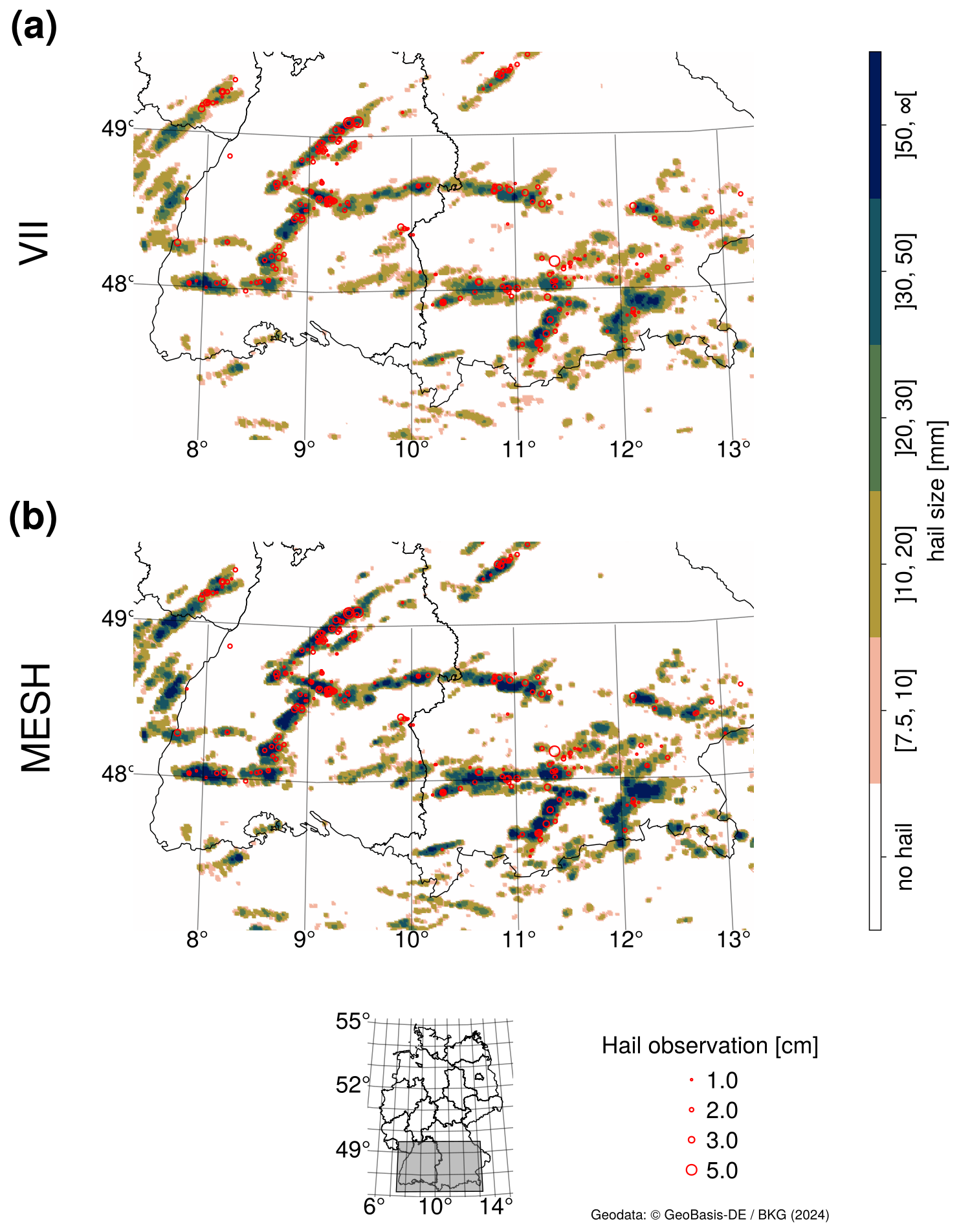
Figure 11 Crowd data from 15 August 2021 zoomed into southern Germany for (a) VII, and (b) MESH.

Generally, we see that the hail track is matched quite well for MESH and VII in comparison to the crowd data. The MESH hail size is larger than the VII hail size. The MESH track shows more areas with small hail sizes. Most of the crowd data are reported within those two tracks, and only a few reports of small hail are located outside the tracks. MESH overestimates the sizes clearly. VII has similar magnitudes of hail size compared to the observations, and the locations also fit quite well. To show a more complete picture for different MESH formulas and VII compared to the observations, we have validated all of those algorithms with hail days in 2024 that were not used for the MESH fitting (see Table A1). From that we can say that VII performs best for hail sizes up to 3 cm. The MESH formula that uses the mean instead of the 75 % percentile is also very good. For larger hail sizes there were only a few observations, but for them, the 75 % formulas for MESH (as well as those of Murillo and Homeyer, 2019, and of our own fit) outperform those for VII. The result is not unexpected because MESH is fitted so that 75 %, 95 % respectively, of the values are lower so that we can be very sure that the resulting hail size is the maximum expected. VII does not try to find the maximum value of hail. For most of the observations (75 %) the MESH value is too large, so overall MESH does not perform as well as VII, especially for smaller hail sizes. For the larger observation values MESH performs better because of the assumption for fitting the formula. Both VII and MESH, therefore, take different aspects of hail size into account. We have chosen VII for a larger analysis over the period 2018–2023, as it fits better for most of the values.

4.6 Multi-annual analysis of VII in Germany

The study covers a relatively short period of 6 years from 2018 to 2023, but nevertheless it can give great insights into the hail distribution across Germany. First, we look at the total number of hail days in the period under review. Figure 12 shows the mean number of hail days from 2018 to 2023 based on VII.

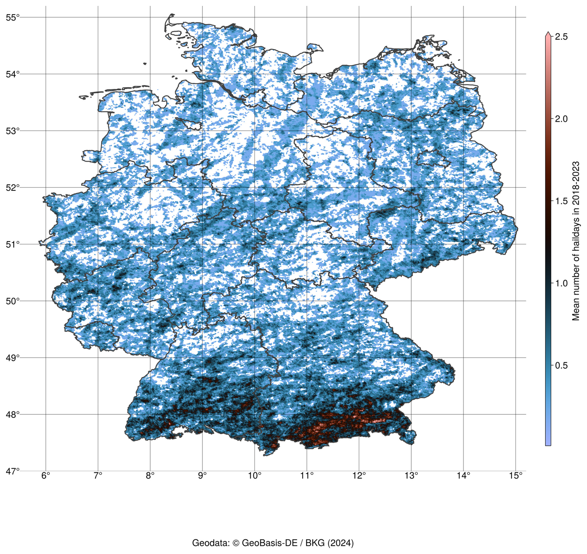
Figure 12 Mean number of hail days in a year based on VII for the period 2018–2023.

The occurrence of hail shows a gradient from north to south with a maximum in the alpine foothills of Bavaria. However, according to the VII approach, 80.6 % of Germany within a 1 × 1 km² area is hit by hail at least once in those 6 years. The mean number of hail occurrences per year is about 0.33; this means approximately 2 hail events in the analyzed period. The maximum number of hail days for one grid cell is 19 d in the time period. The largest number of hail days can be found in the German low mountain ranges in the most southern part. Although Fig. 12 shows that hail is possible everywhere in Germany, hail occurrence and hail size strongly depend on single storm tracks. The number of hail days in 2019, as shown in Fig. 13a, shows hotspots in the eastern part of Germany, contrary to 2021, in Fig. 13b, where there are hotspots in the Pre-Alps. In 2019 only 25 km², compared to almost 900 km² in 2021, had more than 4 hail days in Germany.

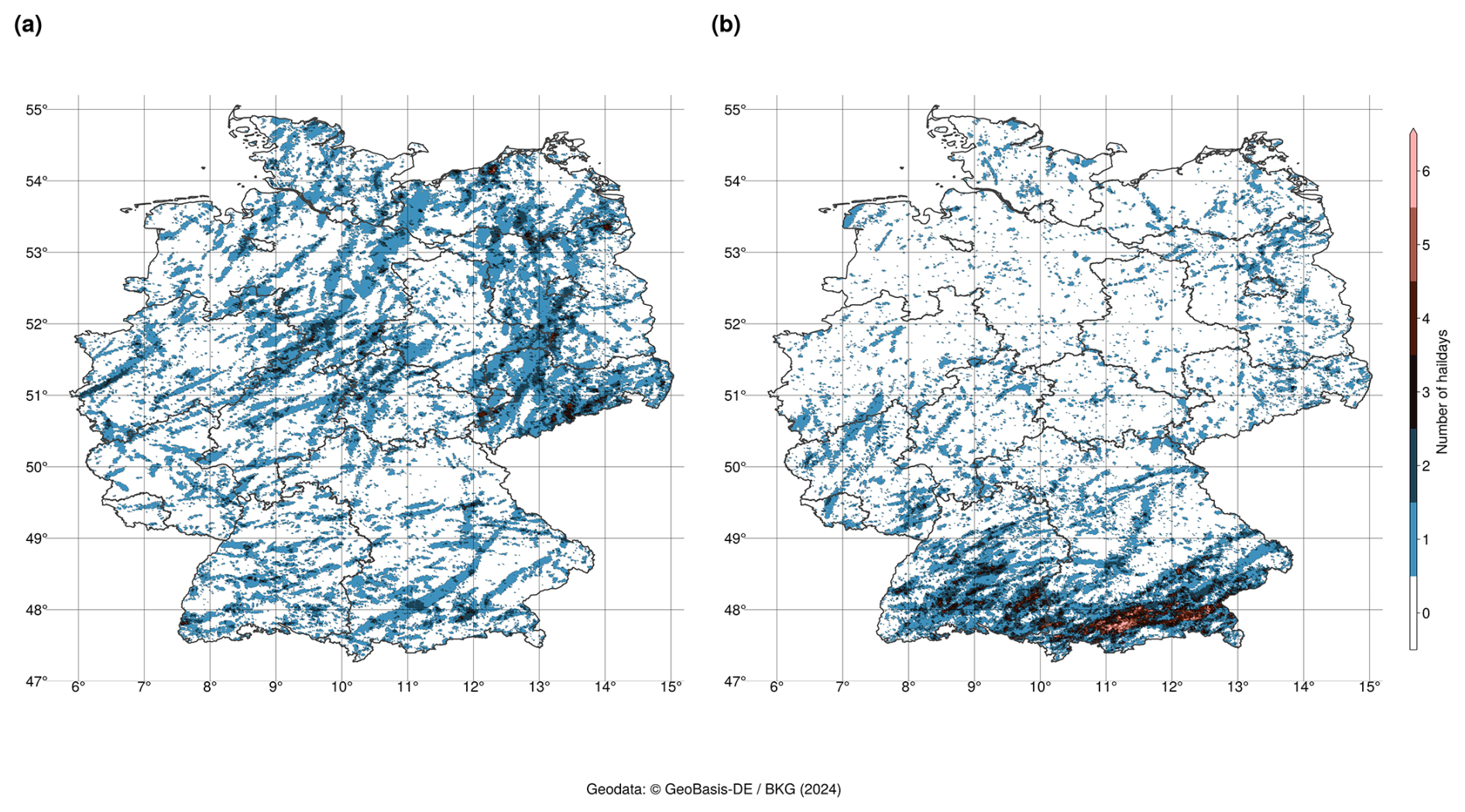
Figure 13 Two examples of the number of hail days based on VII with very distinct hotspots in (a) 2019 and (b) 2021.

Also the maximum hail size in each year is highly influenced by single storms (see Fig. 14). On average, the maximum hail size is about 1.5–3 cm depending the year. Single storms producing clearly visible hail tracks (see Fig. 14a) can also lead to larger hail sizes. One of the largest hail storms in recent years can also be seen in Fig. 14b. The hotspot of maximum hail sizes is situated directly over Kassel (mid-Germany) with hail larger than 7 cm. The area with extreme hail has a large track and a large width.

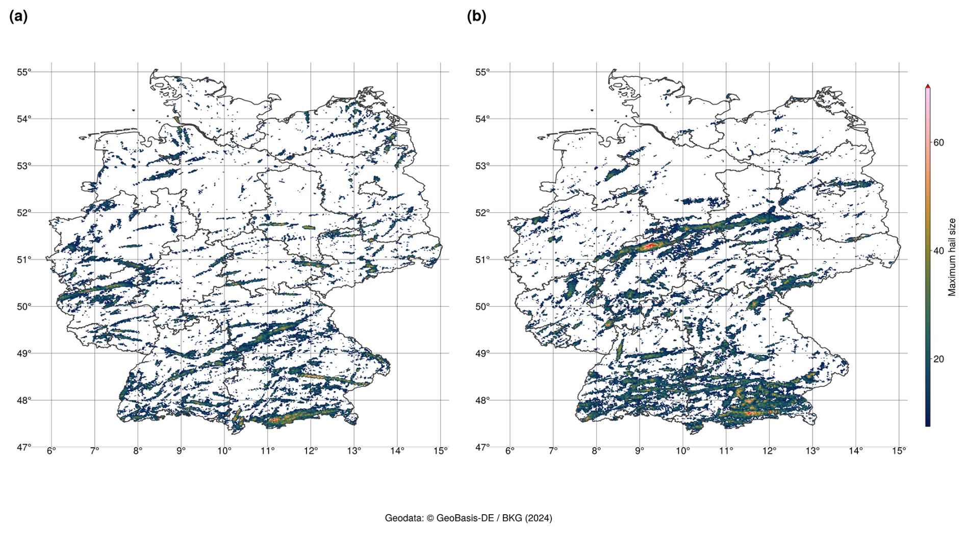
Figure 14 Two examples of the maximum hail size based on VII in (a) 2022 and (b) 2023.

The maximum hail size over the period 2018–2023 is shown in Fig. 15. There are only very few hail days with hailstones larger than 5 cm. Over southern Bavaria, individual cell tracks are discernible, suggesting that the most severe hail events are caused by isolated extreme convective cells. Most of the detected hail sizes are smaller than 2 cm. The occurrence of hail using VII shows a clear annual cycle (see Fig. 16) which is in accordance to the results with crowdsourcing data (Sect. 4.1). From April to June (Fig. 16a–c) the number of hail days increases, with numbers subsequently decreasing again afterwards until September (Fig. 16d–f). Before April and after September, VII cannot detect any reasonable amounts of hail. A similar annual cycle can be observed for the maximum hail size (see Fig. 17). In April (Fig. 17a) there are some hailstorms, but with only small sizes. In May (Fig. 17b) the sizes become larger until the peak in June (Fig. 17c). In the Pre-Alps, large hail also occurred in August (Fig. 17e) during the investigated period.

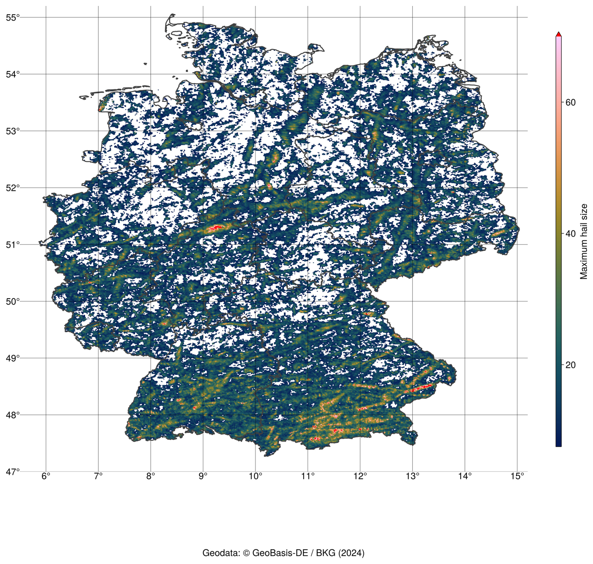
Figure 15 The maximum hail size based on VII for each pixel over 2018–2023.

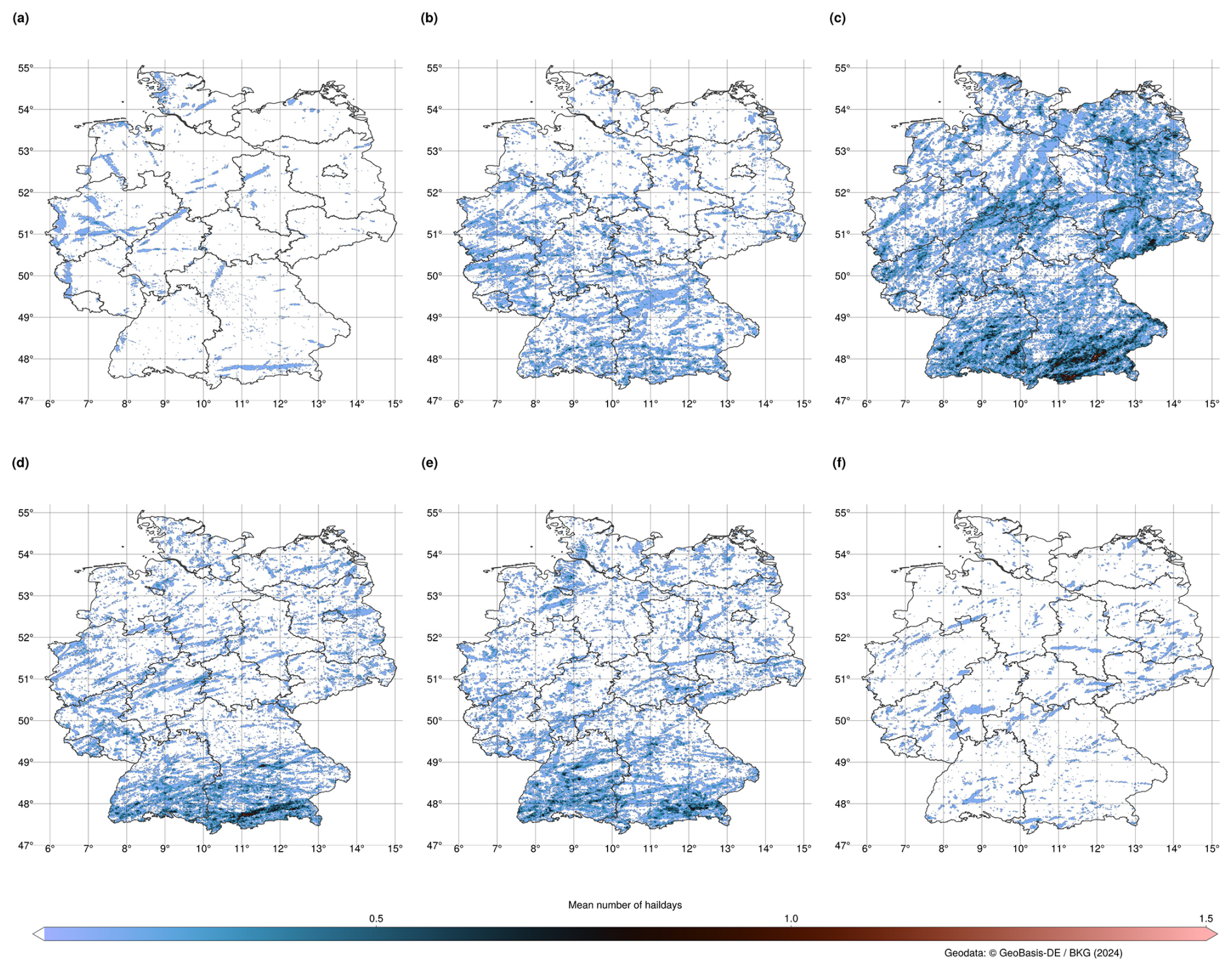
Figure 16 The annual cycle of hail days from 2018 to 2023 in Germany based on VII from (a) April, (b) May, (c) June, (d) July, (e) August and (f) September.

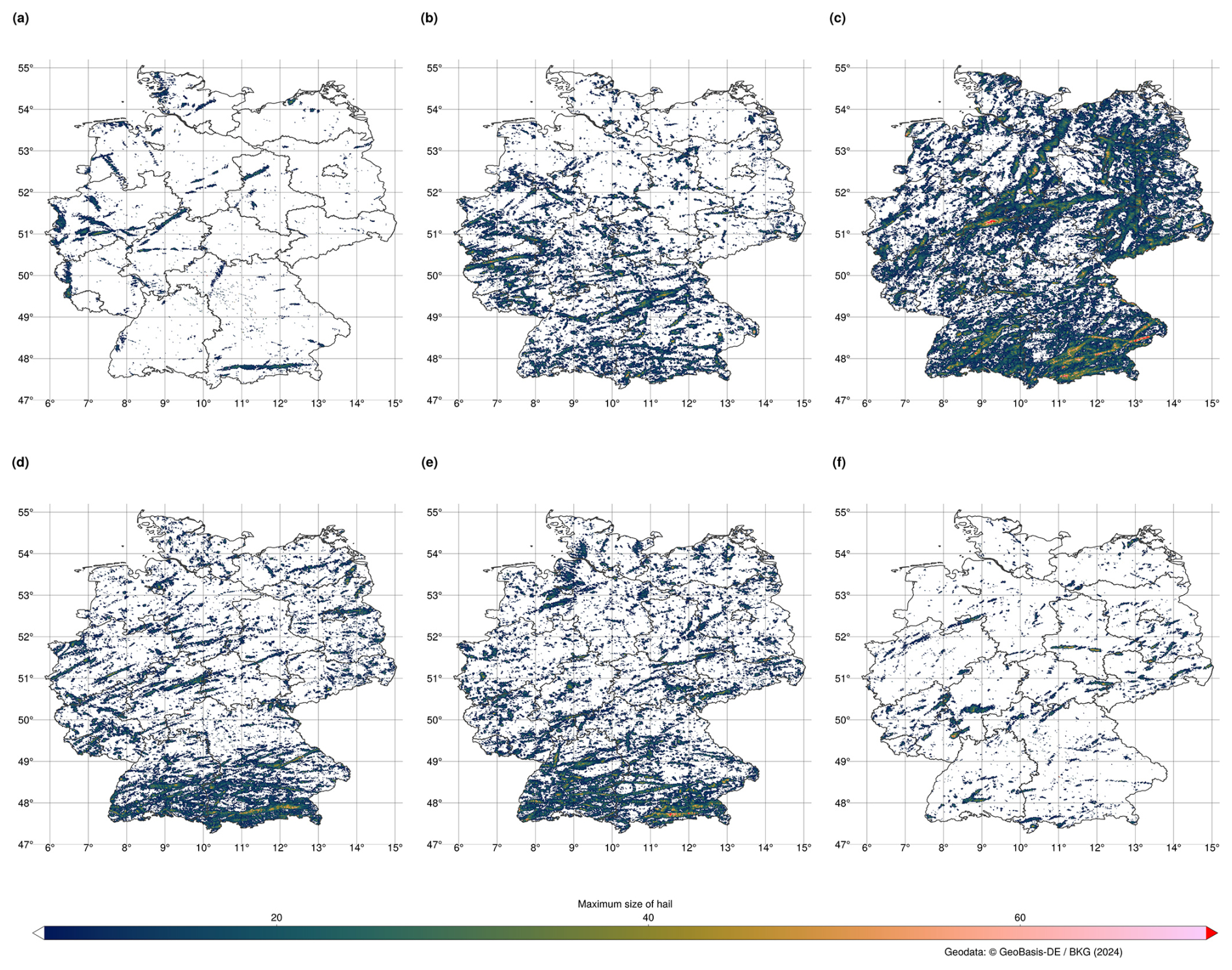
Figure 17 The annual cycle of hail sizes from 2018 to 2023 in Germany based on VII from (a) April, (b) May, (c) June, (d) July, (e) August and (f) September.

4.7 Insurance data

The analysis in Fig. 18 shows that June is the month with the most damage caused by hail, with a mean of 33 972 damage reports. In July, a similar mean number of damages is reported in terms of the number of damage reports, with a mean of 29 492. The hailstorm that occurred in July 2013 had a significant impact on the mean number of damage reports. If 2013 is left out of this analysis, the mean drops to only approximately 15 002 damage reports. The number of reports of damage in April (M = 1509) and September (M = 1228) is relatively low, while in May (M = 9230) and August (M = 11 526) the number of reports is in the midfield. The loss expenses show a very similar picture to the number of damage reports. It is quite interesting that in 2022 the loss expenses in May (EUR 100.43 million) and September (EUR 21.2 million) are much higher than in the years before (May: M = EUR 24.53 million; September: M = EUR 3.18 million). In June, July and August 2022 the loss expenses are on a similar level or smaller.

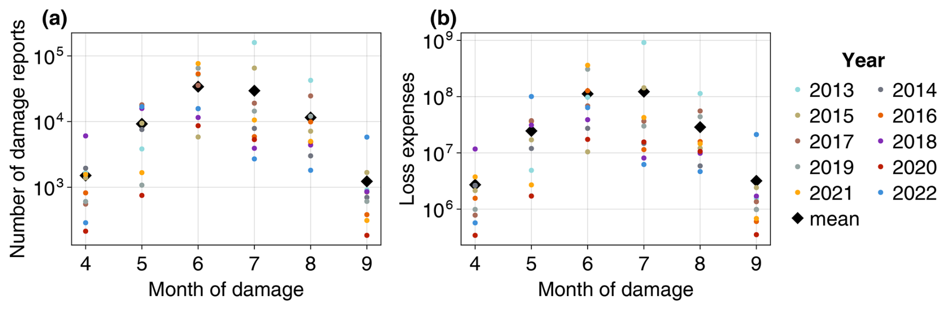
Figure 18 Insurance data for the summer months each year in the period 2013–2022. (a) Number of damage reports. (b) Sum of loss expenses.

We can compare the number of damage reports to the number of observations in total (see Fig. 8) as well as to the distribution of hail sizes (see Fig. 9). Similar results can be found for the loss expenses in place of the damage reports. Both the number of damage reports and the number of hail observations (Fig. 8) show a clear annual cycle with a peak in the summer months, moderate numbers of reports and observations in spring and autumn, and almost no hail events in winter. The maximum number of damage reports, however, occurs in June and July and, therefore, shifted to later in the year compared to the observations with a maximum in May and June. This might be due to the hail size: Fig. 9 indicates that small hail dominates in winter, spring and autumn, while medium sized hail dominates in the summer months, probably leading to enhanced damage. Large and giant hail with the highest damage potential almost exclusively occurs from May to August. If the extreme hail event from July 2013 is omitted in the damage reports, their maximum damage potential occurs in June as well as the maximum for medium to giant hail observations.

5 Summary and future work

As hail is a weather phenomenon that is hard to observe and measure, only a few studies about spatial and temporal patterns for hail in Germany exist. In this study we investigated hail statistics for Germany derived from human observed data and C-band weather radar data using the VII and MESH methods. We used crowdsourced data from the WarnWetter app operated by the DWD, staffed weather stations and ESWD data to analyze mainly temporal patterns of hail occurrence. With the benefit of spatial coverage, radar data were used to overcome the lack of spatial information in human observed data. Insurance data give us a hint about the destructiveness of hail in the measure of loss expenses.

In what follows, we attempt to answer the questions posed in the introduction. Our first focus is on the question “Can we rely on the size estimation in human observed hail data?” The use of human observation data for hail size estimation is challenging. The location, date and time may be more reliable than the actual size of the hail estimate. In our study, we found that the mean of many observations is usually very good, but individual observations can be misleading. If the size is wrongly estimated, it is more probable to be underestimated. Giving a category with a known object for reference in mobile phone applications brings a benefit over freely given values. Furthermore, the number of observations underlies the urban reporting bias, as more observations are reported in areas with higher population. Therefore, human observations should be treated with caution, but can still give us a good first idea of the hail event.

To overcome the problem of urban reporting bias, radar data can be used, but “Are the radar based algorithms VII and MESH suitable for determining hail (size) climatologies for Germany?” Despite the use of the developed relationship between SHI and hail size, MESH clearly overestimates the hail size in comparison with crowdsourced data. VII gives similar hail sizes as human observed data in our case study. Therefore, we used VII for showing maximum hail sizes and hail occurrences in Germany for our study period of 2018–2023.

To answer the question of whether hail events in Germany are rare or frequent natural hazards, we can combine the results from radar data and human observed data. Unfortunately, there is no clear answer to this question because the frequency of hail is quite variable in Germany. Large to giant hail is very rare in Germany. The south of Germany has a higher chance of being hit by large hail and is typically hit more frequently by hail storms than the north. Nevertheless, large hail events are possible all over Germany, such as the hailstorm that occurred in the middle of Germany in 2023. Púčik et al. (2019) and Kaltenböck et al. (2009) used the ESWD data to analyze the diurnal cycle of hail in Europe. Their findings that the diurnal peak of hail occurrence is about 15:00–16:00 UTC can be confirmed with the longer time series of this study for Germany. It must be noted that crowdsourced data are likely biased in terms of the diurnal cycle with an underrepresentation during nighttime hours. Púčik et al. (2019) depicted a similar annual cycle pattern for southern Europe (regions south of 46° N latitude) to the annual cycle found by this study. For regions north of 46° N they found more activity in July. With the VII derived from radar data we clearly see June as the month with the most hail days for whole of Germany.

For crowdsourced data the analysis showed many reports in the highly populated Ruhr and Rhine-Main areas and in the larger cities like Berlin and Munich (urban reporting bias). The hotspot close to Stuttgart (south-west Germany) that was found previously (Puskeiler et al., 2016) can be seen in the VII data.

With the use of radar-based algorithms, we can produce a picture of hail over the whole of Germany. We can confirm the overestimation of MESH, which Brook et al. (2024) overcame with an empirical correction. We have chosen VII for the multi-year analysis, as it better fits the crowd data in our case study in terms of hail size. The case study shows that the hail tracks of MESH and VII fit quite well to the observations.

It is currently not possible to calculate any trends in hail occurrence using only the observation data due to the varying number of observers over the years. The WarnWetter app introduces much more active observers than we had before. The same is true for the ESWD data, which increased in the number of reports made over time. With radar data we see years with a lot of hail, e.g., 2021, and years with little hail, e.g., 2020. Overall, the analyzed period of 6 years is not long enough to define a trend and was outside of the scope of this study. For trend analysis, modeled data (Battaglioli et al., 2023; Wilhelm et al., 2024) might be a better fit when other consistent time series are too short.

A question for the future is to determine the most appropriate metric for determining the severity of hailstorms. Should the largest individual hailstone be used as the benchmark? Alternatively, could we consider an average diameter? What is the ground truth for this approach? An alternative approach would be to omit the exact hail sizes and identify the impact or damages directly (e.g., Schmid et al., 2024). If crowdsourced data are used, it is important to consider the potential biases that may affect the results. The position may be inaccurate, there may be a population bias, and there is a possibility that only large hail is being reported. Additionally, there is an estimation problem and a diurnal cycle for reporting. For future work, it might be interesting to recalculate VII for earlier years to see if there are any patterns or trends in hail occurrence in Germany. Furthermore, the SHI–MESH relationship could be fitted to a longer time series of observed data. For the refitting, the observations could be pooled to use only the mean of neighboring observations and to only take observations into account with neighboring observations available. A similar approach of refitting could be applied to the VII data to increase the performance even further. As we have some diverse data sources, artificial intelligence methods could be beneficial to combine all data sources and result in impacts for the population or hail probability.

Appendix A: Validation of MESH and VII with some case days

Table A1 Statistical analysis for different days with hail in 2024 for MESH fitted with our own data, MESH 75 % by Murillo and Homeyer (2019) and VII compared to data from the WarnWetter app. For the algorithms, the maximum value of the last 15 min before the observation with a radius of 5 km around the observation was taken. Bold values represent the best value for the observation size.

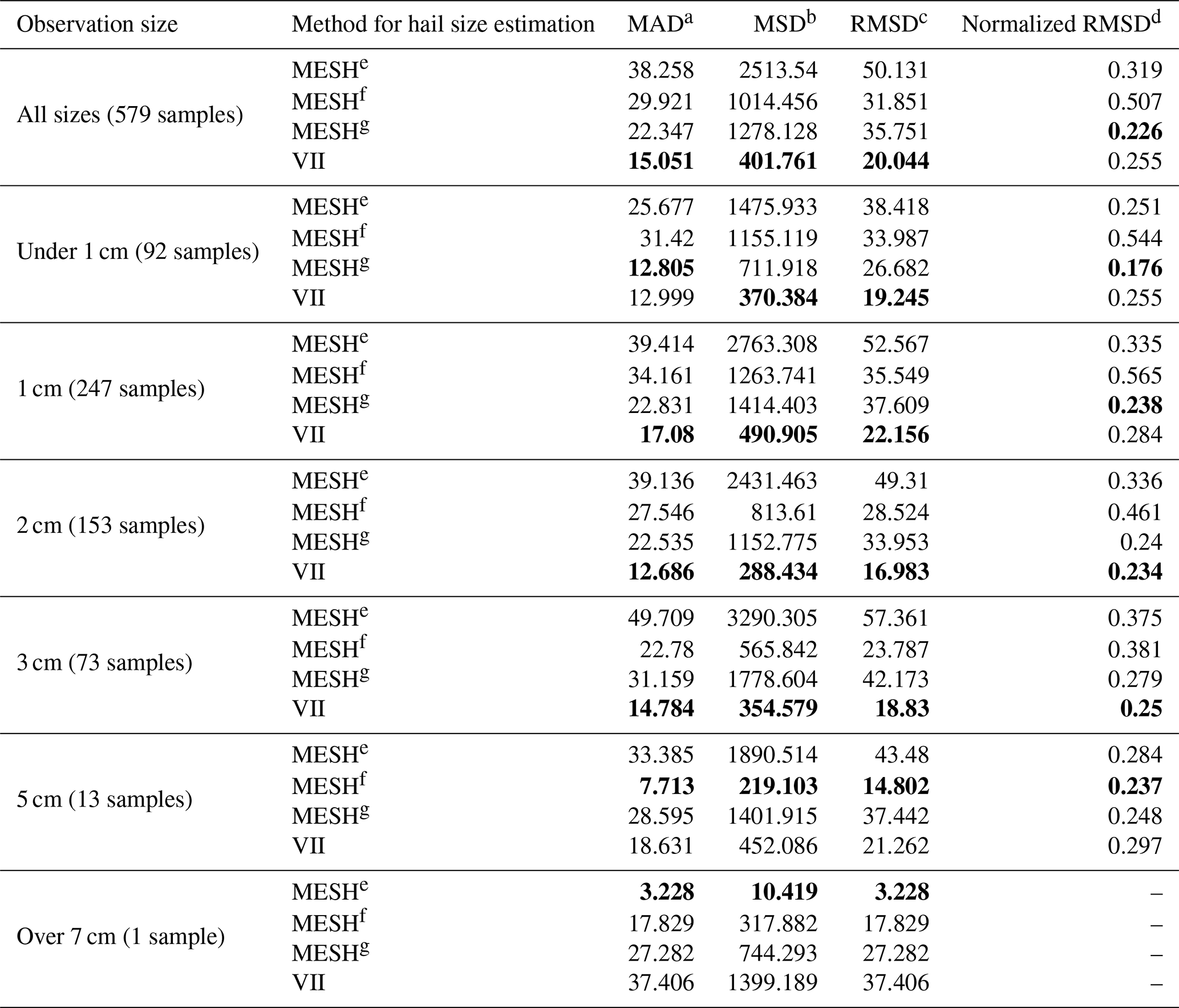
^a Mean absolute deviation. ^b Mean squared deviation. ^c Root mean squared deviation. ^d Normalized root mean squared deviation. ^e MESH from own fitted 75 %. ^f MESH fitted by Murillo and Homeyer (2019) 75 %. ^g MESH from own fitted mean.