The ability of a stochastic regional weather generator to reproduce heavy-precipitation events across scales

We assess the ability of a regional weather generator to represent the extremity of heavy-precipitation events (HPEs) across spatial and temporal scales. To this end, we implement a multi-site non-stationary regional weather generator (nsRWG) for the area of Germany and generate 100 sets of synthetic daily precipitation data spanning 72 years. The weather extremity index (WEI) and its recent cross-scale modification (xWEI) are applied to quantify the cross-scale extremity of synthetic and observed HPEs and to compare their distributions. The results show that the nsRWG excels in replicating the extremity patterns for almost all seven durations (ranging from 1 to 7 d) considered. The frequency of small-scale 1 d rainfall is, however, slightly overestimated. The nsRWG aptly reproduces the potential influential areas of HPEs, whether of a short or long duration. It is capable of generating precipitation events mirroring the extremity patterns observed during past disaster-causing HPEs in Germany, while simultaneously accommodating their variations. This study demonstrates the potential of the nsRWG for simulating HPE-related hazards and assessing flood risks.

1 Introduction

Heavy-precipitation events (HPEs) are rare weather phenomena which accumulate exceptional amounts of rainfall, within hours to days, over areas ranging from a few to tens of thousands of square kilometers. As the main cause of damaging floods and landslides, HPEs are the costliest natural disasters in Europe (Gvoždíková et al., 2019; NatCatSERVICE, 2023; Swiss Re Institute, 2024). Climate change is expected to increase the frequency, intensity, and spatial extent of HPEs (Christensen and Christensen, 2003; Lenderink and Fowler, 2017; Matte et al., 2022; Yang et al., 2023) and their associated impacts (Merz et al., 2021).

Germany has experienced several notable HPEs in recent years (Hu and Franzke, 2020). For example, in August 2002, heavy precipitation led to record-high water levels in the Elbe River and its tributaries (Kreibich et al., 2017; Thieken et al., 2022). In July 2021, a widespread HPE hit the western and southern parts of Germany as well as neighboring countries and caused one of the most devastating flood events in German history, with more than 180 fatalities and EUR 33 billion in damages (Apel et al., 2022; Szönyi et al., 2022; Mohr et al., 2023).

To understand the physical mechanisms and to assess the potential consequences of HPEs, analyses of past events can be carried out (e.g., Caldas-Alvarez et al., 2022; Mohr et al., 2023). Alternatively, large ensembles of climate model simulations (e.g., Ehmele et al., 2022) or synthetic weather fields can be generated to extract a set of plausible HPEs. The latter option represents a more computationally efficient approach by deploying stochastic weather generators (WGs). WGs are stochastic models that are capable of generating synthetic spatiotemporal fields of weather variables such as precipitation, temperature, and humidity, retaining the statistical properties of observed or climate model data on which WGs are conditioned, such as autocorrelation, spatial covariance, and multi-variable dependence. A large number of WG models have been introduced so far, based on various statistical methods; among others, reshuffling and perturbing analogue weather fields or applying multi-variate auto-regressive models (for a review, see Maraun et al., 2010; Haberlandt et al., 2011; Serinaldi and Kilsby, 2014; Benoit and Mariethoz, 2017; Nguyen et al., 2021). WGs can be instrumental in generating synthetic HPEs, thereby supporting flood risk management and climate adaptation (Breinl et al., 2013; Chen and Brissette, 2014; Harris et al., 2014; Sairam et al., 2021). WGs are widely used for estimating hydrological design values (Winter et al., 2019), downscaling climate model output (Fatichi et al., 2011; Kiem et al., 2021), climate impact assessments on water resources (Harris et al., 2014; Najibi et al., 2024), and flood risk assessments (Sairam et al., 2021), providing long-term datasets for scenarios where observational data may be limited and where downscaled future climate projections are needed. WGs are particularly effective when integrated with other models to better understand and prepare for HPEs and their consequences (Mehrotra and Sharma, 2010; Zhou et al., 2020). For instance, long-term synthetic weather fields (like precipitation and air temperature) generated by WGs can be used as meteorological forcing for hydrological models in order to quantify HPE-related floods and damages (Apel et al., 2016; Qin and Lu, 2014; Sairam et al., 2021). This approach allows researchers to develop exceptional flood events needed for flood design or disaster management planning, as the generation of very long time series of flood flows and inundation increases the probability of obtaining situations where the unfortunate superposition of the different flood-generating processes leads to severe impacts (Falter et al., 2015). Such situations are rarely encountered in measured time series that are usually very limited in length.

Evaluating the performance of a WG is crucial to ensure that it accurately represents historical weather data and produces synthetic weather sequences that are adequate for the application context, e.g., flood estimation, drought assessment, climate change impact assessment (Tseng et al., 2020). The evaluation process helps to identify biases or limitations in the model output and fosters model improvements (e.g., Breinl et al., 2013; Serinaldi and Kilsby, 2014; Nguyen et al., 2021). Widely used metrics to evaluate synthetic precipitation data include the mean, standard deviation and skewness, lag-1 autocorrelation, frequency of wet (or dry) days, and precipitation intermittency (Steinschneider and Brown, 2013; Tseng et al., 2020; Zhou et al., 2020; Nguyen et al., 2021). Additionally, the performance of WGs in simulating the extremity of precipitation events is of special interest. The extremity of precipitation events is usually described by intensity, duration, and spatial extent statistics (Beniston and Stephenson, 2004; Jeferson de Medeiros et al., 2022; Müller and Kaspar, 2014; Zhang et al., 2011). The spatial consistency of multi-site WGs is sometimes evaluated based on the areal mean of the synthetic field within a region, e.g., the average rainfall of the catchment (Ullrich et al., 2021). However, this method may underrepresent the variability in the affected area, particularly when calculated in a fixed region, as the areal mean underestimates the extremity when only part of the region is heavily affected (Müller and Kaspar, 2014; Voit and Heistermann, 2022). To address these issues, the correlation between multiple sites can be used to measure the spatial dependence structure of the precipitation amount across a region (Breinl et al., 2013; Gao et al., 2021; Tseng et al., 2020). Furthermore, the continuity ratio, expressed as the ratio between the average precipitation at one location when another location is dry or wet, can capture the spatial coherence of precipitation between adjacent locations (Wilks, 1998; Breinl et al., 2013). However, both the correlation coefficient and the spatial continuity ratio are dominated by the bulk of the precipitation events rather than by the extreme values.

HPEs can vary in duration, from short intense downpours to prolonged periods of heavy rainfall. Quantile-based thresholds of block maxima of precipitation totals and empirical probability distribution plots are typically used to characterize WG performance for extremes (Breinl et al., 2013; Zhou et al., 2020; Nguyen et al., 2021; Ullrich et al., 2021). Such methods are usually applied separately for different durations, neglecting the temporal coherence of HPEs, which in reality can be simultaneously extreme at different temporal and spatial scales, triggering different types of flooding overlaying each other (Ramos et al., 2017). For instance, during the 2002 Elbe flood, small-scale extreme precipitation caused flash floods in several small Elbe tributaries. During the same event, extreme rainfall over large spatial scales and longer durations triggered fluvial flooding, with widespread inundation and finally long-lasting groundwater flooding in the city of Dresden (Kreibich et al., 2005; Thieken et al., 2022). The ability of WGs to represent these cross-scale characteristics of precipitation events is thus essential for flood risk modeling. Up to now, no single measure has been used to evaluate the ability of WGs to capture the cross-scale extremity of rainfall.

In this study, we demonstrate a new evaluation approach for a WG based on the weather extremity index (WEI; Müller and Kaspar, 2014) and the cross-scale weather extremity index (xWEI) introduced by Voit and Heistermann (2022). These indices quantify the extremity of an event, considering different duration levels and spatial extents. xWEI additionally integrates the extremity over different duration levels and spatial extents. Our aim is to evaluate how well the cross-scale extremity of precipitation events is captured by a WG, even if it is not specifically tailored or trained to do so.

2 Study area and data

The study area is Germany (Fig. 1), given its exposure to hazards induced by heavy-precipitation events (HPEs), as highlighted in the introduction. A non-stationary regional weather generator (nsRWG) (Nguyen et al., 2024) is implemented for the whole of Germany and parts of the upstream neighboring countries, covering the five major river catchments – Elbe, Rhine, Danube, Ems, and Weser – to produce long-term spatially consistent synthetic precipitation and temperature data. In this study, we focus on the ability of the WG to represent the extremity of precipitation across scales. Weather generators that comprise several catchments and cover such a large spatial area (more than 650 000 km²) are rare, and previous studies have commonly implemented WGs at smaller scales (Tseng et al., 2020; Ullrich et al., 2021; Gao et al., 2021).

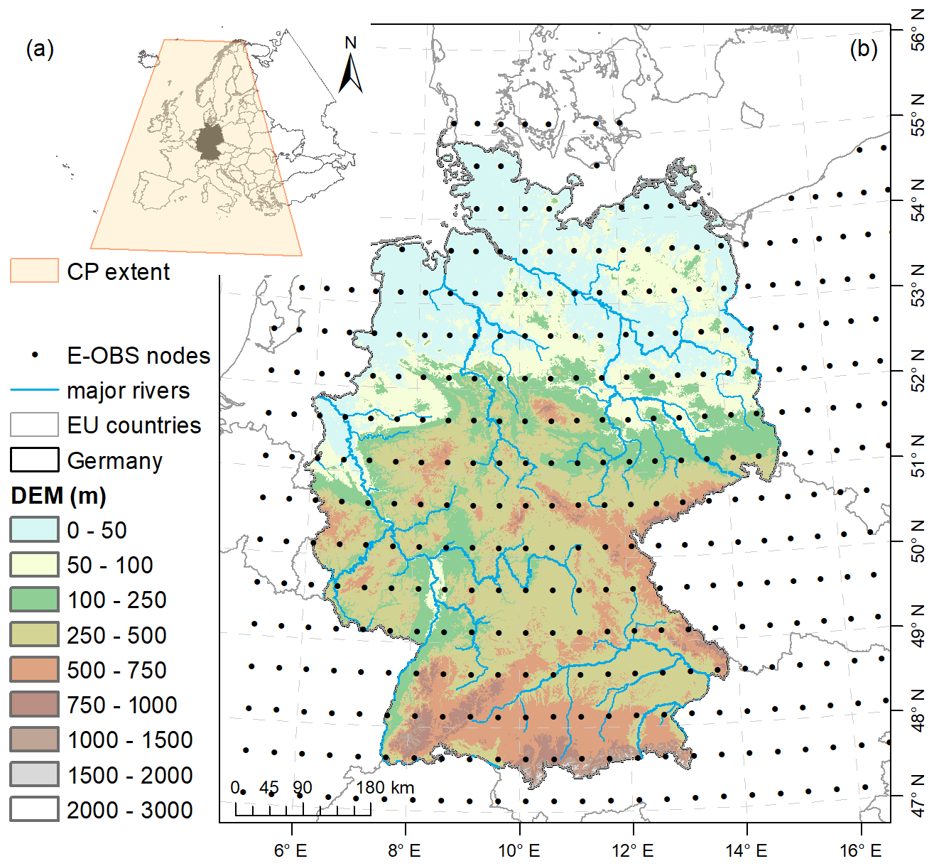
Figure 1 The study area (Germany and adjacent regions) and its topography, major rivers, and E-OBS grid nodes. The extent of where the mean sea level pressure was extracted to classify the circulation patterns (CPs) is shown in panel (a).

Two datasets are used to parameterize the nsRWG: (1) gridded precipitation data from E-OBS (version 25.0e; Cornes et al., 2018) and (2) mean sea level pressure and daily air temperature at a 2 m height from the ERA5 reanalysis (Hersbach et al., 2020). Mean sea level pressure is used to classify circulation pattern types for which the local distributions of precipitation are conditioned. Regionally averaged daily temperature acts as a covariate of the local distribution in order to consider changes in precipitation for the same circulation pattern in a non-stationary warming world (Nguyen et al., 2024). Both the E-OBS and ERA5 datasets are available at a daily resolution, spanning from 1 January 1950 to 31 December 2021.

E-OBS is an ensemble gridded weather dataset and is available on a regular 0.25° grid, covering Europe. It is based on station data collated by the European Climate Assessment & Dataset initiative (Cornes et al., 2018). To cope with the high computational demands, we have resampled the grid points to a reduced spatial resolution of 0.5°. The locations of the extracted E-OBS grid points are given in Fig. 1.

The ERA5 dataset, provided by the European Centre for Medium-Range Weather Forecasts (ECMWF), is a state-of-the-art reanalysis dataset widely used in climate research (Hersbach et al., 2020). It provides a comprehensive and detailed representation of atmospheric conditions at the global scale. To classify the large-scale atmospheric situation, mean sea level pressure is extracted over an extent (25–70° N ,  15° W–30° E; see Fig. 1a) that encompasses a substantial portion of Europe and adjacent regions. The regional average 2 m daily air temperature is computed for the domain 45.125–55.125° N and 5.125–19.125° E, which covers the nsRWG setup area.

3 Methods

3.1 A stochastic multi-site non-stationary regional weather generator (nsRWG)

We adopt the non-stationary version of the multi-site regional weather generator nsRWG developed by Nguyen et al. (2024). The nsRWG represents the spatiotemporal dependence across sites using the first-order multi-variate auto-regressive (MAR-1) model (Bardossy and Plate, 1992). The type-1 extended generalized Pareto (extGP) distribution is used to model daily non-zero precipitation amounts. This distribution is suitable not only for capturing both the lower bulk of precipitation amounts and the extreme values but also for providing a smooth transition along the precipitation range (Naveau et al., 2016; Nguyen et al., 2021).

In the nsRWG, the precipitation distribution at each site is conditioned on the large-scale circulation pattern as a latent variable and the regional average daily temperature as a covariate of the extGP distribution scale parameter. In this way, climate variability and climate change due to changes in dynamic and thermodynamic properties of the atmosphere are considered. Atmospheric circulation is classified into six circulation patterns based on mean sea level pressure for the winter (1 November–30 April) and summer (1 May–30 October) seasons (12 patterns in total). We use the objective classification algorithm Simulated ANnealing and Diversified RAndomization (SANDRA) based on the k-means clustering approach (Philipp et al., 2007) for circulation pattern classification. Further details about the nsRWG algorithm and configuration can be found in Nguyen et al. (2024).

The cross-scale precipitation performance of the nsRWG is evaluated for the E-OBS grid cells in the study area for the period from 1 January 1950 to 31 December 2021. We generate 100 realizations of synthetic precipitation datasets with a time series length of 72 years, corresponding to the length of the E-OBS dataset to ensure comparability.

3.2 WEI and xWEI

The weather extremity index (WEI) quantifies the extremity (a product of spatial extent and rarity) of an event, as well as the spatial extent and temporal duration at which the event reached its maximum extremity (Müller and Kaspar, 2014). In this context, the spatial extent of an event is not conceived as an area of spatially contiguous grid cells but as a number of (potentially disjoint) cells in the study region (here, Germany) that exceeds a certain return period. The computation of WEI for individual HPEs is illustrated in Fig. 2. For a given spatial domain (in this case, Germany), it starts with the estimation of the return periods P_t,i at each grid cell i for durations from 1 to t days. For each duration t, the grid cells in the spatial domain are sorted in decreasing order, based on their return period P_t,i (in years) and then aggregated over increasing areas A (in km²) by using Eq. (1): first, E_t,A is computed for the most extreme grid cell (n = 1). Then, the following grid cells are added to the computation of E_t,A, increasing the value of n by 1 until the estimated return period from every grid cell is computed once. For each step, the area A equals the area of one single grid cell multiplied by n. In the final step, A corresponds to the size of the entire spatial domain. Finally, this procedure yields, for each duration t, a curve that shows E_t,A as a function of A. The value of WEI is then defined by the maximum value of E_t,A for all curves, and the spatial extent and duration at which the event was most extreme corresponds to the values of t and A, for which this maximum of E_t,A is achieved. Note that the E_t,A curves typically have a well-defined maximum: for low values of A, the steep increase of $\sqrt{A/\mathit{\pi }}$ (the radius of a circle of size A) causes an increase of E_t,A with A. For larger values of A, the decrease in return periods dominates the behavior and causes the E_t,A curve to decrease. The corresponding area where the E_t,A curve reaches its peak (WEI) is denoted here as WEI area, which represents the spatial scale most severely affected by the HPE. The WEI area is always much smaller than the area over which the HPE precipitation totals exceed 0 mm. Rather, it is a weighted measure indicating the area in the domain that is heavily influenced by the HPE and hence prone to HPE-related impacts.

$$\begin{array}{}\text{(1)}& E_{t,A}={\displaystyle \frac{{\sum }_{i=\mathrm{1}}^n\ln \left(P_{t,i}\right)}{n}}\cdot \sqrt{A/\mathit{\pi }}A=\text{grid size}\times n\end{array}$$

As each E_t,A curve represents how the extremity of an event extends across spatial scales, Voit and Heistermann (2022) proposed a cross-scale weather extremity index (xWEI) by integrating E_t,A over duration (ln (t)) and extent (A). xWEI quantifies how much the extremity of an event extends across both space and time (instead of the event just being extreme at one specific duration and extent). Hence, xWEI corresponds to the volume under the surface which is spanned by the E_t,A curves (Fig. 2f) and placed on a grid:

$$\begin{array}{}\text{(2)}& \text{xWEI}=\int \int E_{t,A}\mathrm{d}A\mathrm{d}\left(\ln \right(t\left)\right).\end{array}$$

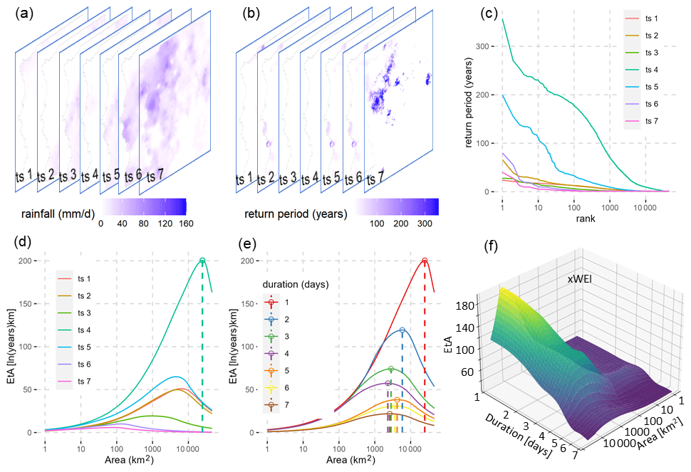
Figure 2 Calculation of the WEI and xWEI for an exemplary HPE: (a) maps of daily rainfall for a precipitation event lasting 7 d, (b) return period at each individual grid cell of each map, (c) sorting of the return period estimates for each duration in decreasing order for each map, (d) calculation of the E_t,A curves and selection of the curve with the highest peak to represent the extremity pattern of the precipitation for the duration of 1 d, (e) repetition of the procedures (a–d) for other durations (2, 3,…, 7 d) to derive the E_t,A curves, and (f) 3D interpolated surface of E_t,A for all durations and extents. xWEI is defined as the volume beneath the E_t,A surface.

For the exemplary HPE shown in Fig. 2, the analysis highlights the fact that the daily extremity (in terms of 1 d rainfall intensity) occurs on the fourth day, with the highest E_t,A curve among the 7 d (Fig. 2d). Comparing extremity across durations, the HPE is most extreme for a 1 d duration, affecting an area of over 10 000 km² (WEI area). For longer durations (≥ 3 d), the HPE consistently is extreme approximately for the same areas, showing a stabilization in spatial extent for these durations.

To estimate the return periods required to obtain E_t,A, we use the generalized extreme value (GEV) distribution, which has been found suitable for modeling precipitation extremes (Fowler and Kilsby, 2003) and has also been used in previous WEI studies (Gvoždíková et al., 2019; Minářová et al., 2018; Müller and Kaspar, 2014). The computation of xWEI requires return periods for multiple durations (1 to 7 d in our case). We use the duration-dependent GEV (dGEV) method (Koutsoyiannis et al., 1998) to estimate the return periods consistently across durations for each grid cell. Previous studies have shown that this method preserves the tail behavior of precipitation extremes across durations and modifies the scale and location parameters of the GEV distribution to explicitly account for dependency on the duration of events. This allows for more accurate modeling of precipitation intensity–duration–frequency relationships and reduces the uncertainty (Ulrich et al., 2020; Fauer et al., 2021). The parameters of the dGEV distribution at each grid cell are obtained by maximum likelihood estimation using the R package IDF (Ulrich et al., 2021) based on the annual maximum series of rainfall across considered durations.

To assess the extremity of HPEs across Germany, durations from 1 to 7 d are selected, as they are sufficient in capturing the events responsible for disastrous flood damage in the region (Ganguli and Merz, 2019). While WEI and xWEI can be extended to sub-daily scales (Voit and Heistermann, 2022), this analysis is conducted at the daily scale due to the limited availability of sub-daily precipitation observations. Additionally, short-duration high-intensity precipitation events usually affect comparatively small areas, whereas multi-day HPEs span larger regions and are more relevant for this study (Lengfeld et al., 2019, 2021; Orlanski, 1975).

The most extreme HPEs for these seven durations across Germany are identified by extracting the annual maximum WEI values for each duration based on E-OBS precipitation data for the historical period 1950–2021. The corresponding WEI areas (the area where the E_t,A curve reaches its peak WEI) of the most extreme HPEs annually for each duration are categorized into six classes (Fig. 3) in order to analyze the spatial properties of HPEs in Germany. The same procedure is carried out for each of the 100 realizations to evaluate the performance of the nsRWG in reproducing the cross-scale properties of HPEs in Germany.

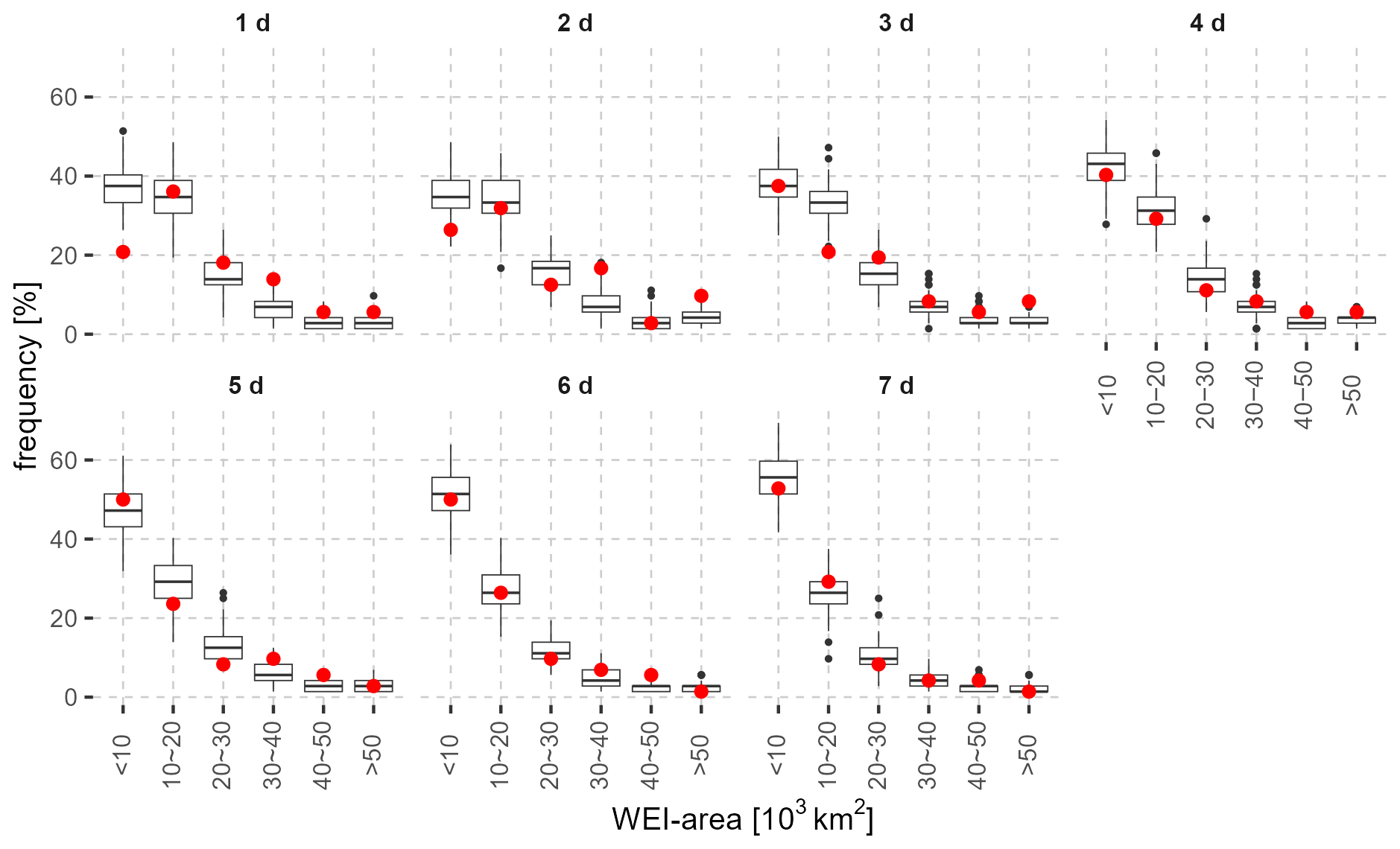
Figure 3 Frequency distribution of observed and nsRWG-simulated WEI areas of the annual maximum HPEs in the period 1950–2021 for seven durations. The titles of the subplots are the durations of interest. The red dots denote the frequency of HPEs in different area categories from E-OBS precipitation data, and the boxplots represent the simulated frequency distribution from the 100 nsRWG realizations.

4 Results and discussion

4.1 nsRWG performance for WEI

Figure 3 shows the frequency distribution of the observed (E-OBS) and simulated (nsRWG) WEI areas of the annual maximum HPEs for seven different durations. The distributions of the annual maximum WEI values are given in Fig. 4. The results show that more than half of the annual maximum HPEs in Germany are events with WEI areas ≤ 20 × 10³ km² for all durations. HPEs with a larger spatial extent of 20 × 10³ km² or more have a frequency of less than 20 % in the past 72 years. However, these events are the most severe ones regarding their WEI values (Fig. 4). The nsRWG is able to reproduce the annual maximum WEI and its corresponding areas for the seven durations. The boxplots in Figs. 3 and 4 show that the simulated distribution patterns are in good agreement with the E-OBS observations. However, for shorter durations (1 and 2 d), the frequencies of HPEs with WEI areas ≤ 20 × 10³ km² are overestimated, while those with larger WEI areas are underestimated (Fig. 3). For durations of 3 d and longer, the observed and simulated HPE frequencies are more balanced.

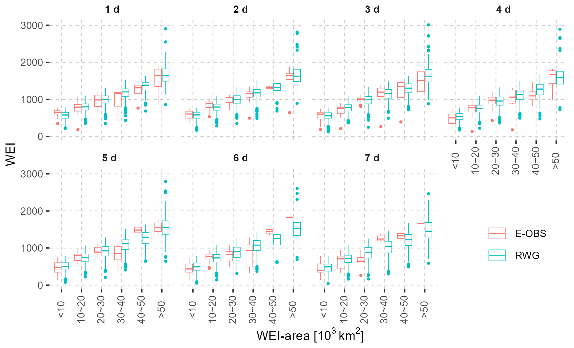
Figure 4 Distribution patterns of observed (red) and nsRWG-simulated (blue) annual maximum WEI series (denoted in the y axis, with the same unit as E_t,A: ln(years) ⋅ km) for seven durations. The WEI areas of HPEs are categorized into six classes (see the x axis).

The relation between the annual maximum WEI values and their return periods derived from the nsRWG data agrees well with the E-OBS observations for the seven durations (Fig. 5). This comparison confirms the ability of the nsRWG to simulate the occurrence probability of HPEs in Germany. The observed probability plots (red dots in Fig. 5) are well enclosed by the simulated ranges (shaded areas) from the nsRWG realizations. This is especially true for high-return periods, which demonstrates the good performance in simulating HPEs for different durations. For short durations and return periods of between 2 and about 10 years, as well as for durations longer than 4 d with return periods between 10 and 20 years, the nsRWG slightly underestimates the observed WEI. In contrast to traditional intensity-duration-frequency curves, there is no systematic difference between the empirical probability plots of the annual maximum WEI series of different durations, as the WEI is based on return periods rather than precipitation totals or averages. This makes the WEI comparable across temporal scales. For example, for HPEs with the same WEI values, the return period increases with duration. This indicates that the occurrence probability of an HPE with the same extremity becomes smaller with increasing duration.

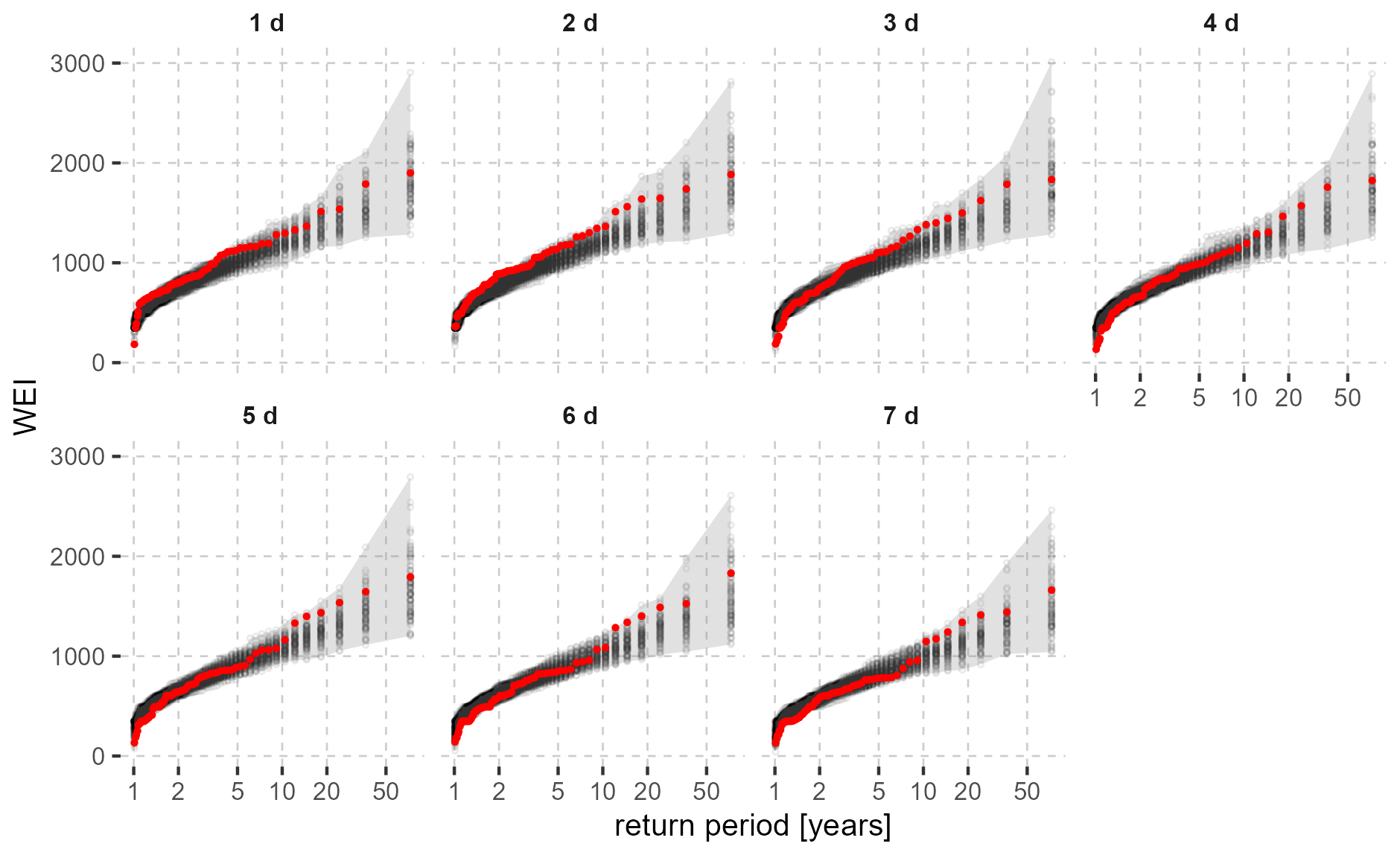
Figure 5 Empirical probability plots of E-OBS observed (red dots) and nsRWG-simulated (black dots) annual maximum WEI for seven durations. The Weibull plotting positions (Makkonen, 2006) are used to estimate the return periods. The gray shaded areas indicate the upper and lower boundaries of the nsRWG simulations.

4.2 nsRWG performance for xWEI

We compute the xWEI for HPEs in Germany for the period 1950–2021 and extract the annual maximum series from both the E-OBS dataset and the nsRWG realizations. The empirical probability plots of annual maximum xWEI, based on Weibull plotting positions (Makkonen, 2006), agree well for both datasets: the cross-scale extremity index xWEI of the observed data lies within the range of the 100 realizations (Fig. 6). However, for return periods between 2 and 5 years, the realizations of the nsRWG tend to underestimate the xWEI, similar to the performance of the WEI.

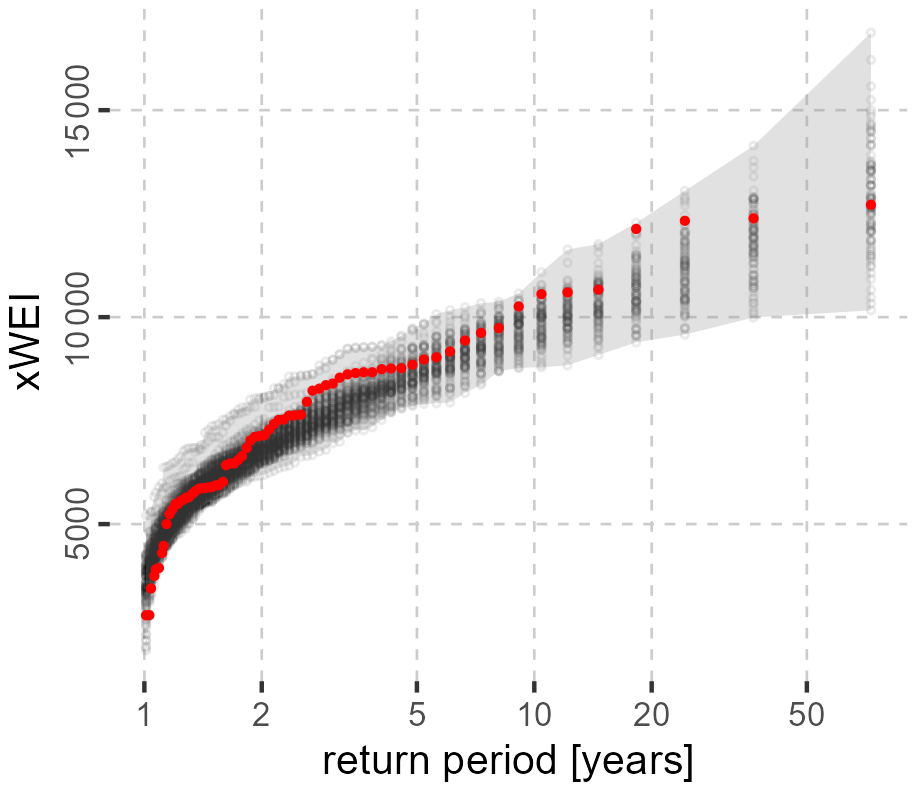
Figure 6 Empirical probability plots of observed (E-OBS, red dots) and simulated (nsRWG, black dots) annual maximum xWEI. The Weibull plotting position is used to estimate the empirical return periods. The gray shaded area indicates the upper and lower boundary of simulated xWEI from the 100 nsRWG realizations.

Figure 7 shows the extremity pattern of a real HPE in August 2002 – one of the most damaging events in Germany. In addition, HPEs from the nsRWG realizations with similar xWEI values to the August 2002 HPE are shown. Fig. 7b demonstrates that the nsRWG is able to generate HPEs with spatial and temporal extremity patterns that are very similar to the August 2002 event, characterized by the highest extremity for the durations of 1 and 2 d and an affected area of approximately 20 000 km². The other two nsRWG-generated HPEs with xWEI values similar to the August 2002 event show different cross-scale extremity patterns (emphasis on longer durations of 3–4 d). The reproducibility of historical HPEs illustrates the ability of the nsRWG in representing the cross-scale extremity of HPEs in Germany. The variations in synthetic events and the respective E_t,A surfaces further demonstrate how the nsRWG can generate synthetic events, which are similar in terms of their cross-scale extremity but have their emphasis at different spatial and temporal scales.

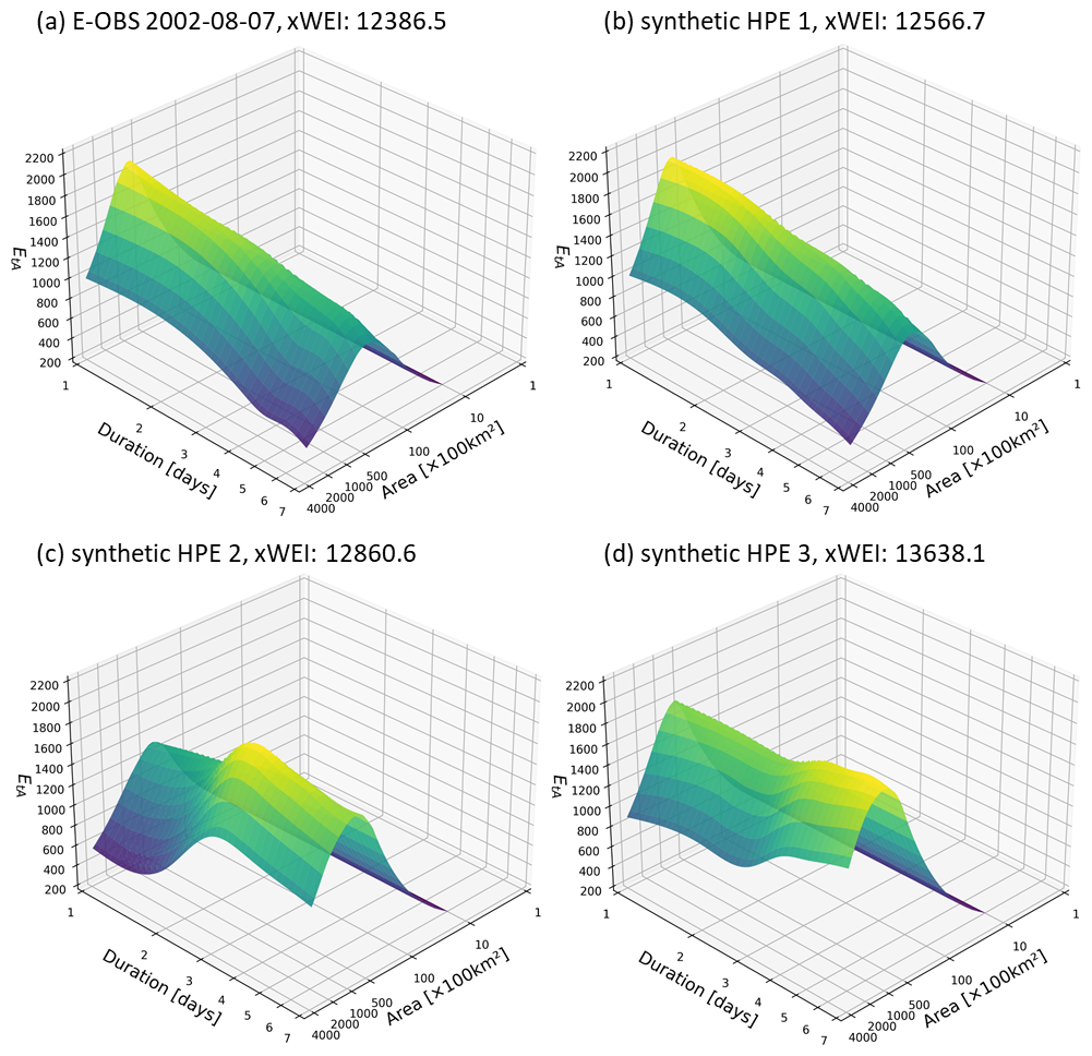
Figure 7 Cross-scale extremity pattern (interpolated E_t,A curves over duration and area) of HPEs for (a) the August 2002 event and (b–d) three HPEs with similar xWEI values generated by the nsRWG. The HPE in panel (b) shows great similarity in the cross-scale extremity pattern with the August 2002 event in panel (a), while the HPEs in panels (c) and (d) display different extremity patterns, although their xWEI values are similar to the actual event in August 2002.

5 Conclusions

In this study, we evaluate the ability of a multi-site stochastic regional weather generator to capture the extremity of HPEs across spatial and temporal scales. For this purpose, we set up the nsRWG at a large scale (covering all of Germany and riparian regions) and generate 100 realizations of 72 years of synthetic precipitation data at a daily resolution. The performance evaluation of the nsRWG in simulating precipitation focuses on the event scale and extreme cases. This focus complements typical proxy statistics (like mean and standard deviation) that tend to represent only the general properties of WGs in precipitation generation. Two indices, WEI and xWEI, are used to measure the extremity of observed and synthetic HPEs, both of them based on the spatial aggregation of return periods of precipitation totals for several durations of interest. While WEI quantifies the maximum extremity of an event that occurred at a specific spatial extent and temporal duration, xWEI integrates extremity across the spatial and temporal scales of interest. The results demonstrate that the nsRWG performs well in simulating the extremity patterns across most spatial and temporal scales of HPEs in Germany. However, it tends to overestimate the frequency of events with short durations and relatively small spatial extents. Using the August 2002 event as an example, we illustrate how the nsRWG is able to generate precipitation events with spatiotemporal extremity patterns similar to those of historical disaster-causing HPEs.

With regard to future research, we emphasize that the choice of the spatial domain at which WGs are evaluated (here, all of Germany) is always a trade-off: on the one hand, the impacts of HPEs unfold at the catchment scale, and it would be an obvious next step to evaluate the ability of the WG to reproduce the frequencies of WEI and xWEI occurrence at the scale of specific river catchments (at the cost of computational effort, as this would require a higher spatial resolution). On the other hand, we need to be aware that an HPE that occurred in one catchment may potentially also occur in a neighboring catchment, so that an analysis at a larger spatial domain (than the present one) is certainly warranted. Such considerations also show the links to “spatial counterfactuals”, which have recently gained attention (Merz et al., 2024; Voit and Heistermann, 2024; Vorogushyn et al., 2025). Counterfactuals are scenarios that describe alternative ways of how an event could have unfolded (Woo, 2019; Montanari et al., 2024). These scenarios could involve conditions where specific factors, such as anthropogenic climate change, natural climate variability, or other boundary conditions, are altered or removed (Gauch et al., 2020). Spatial counterfactuals are a special case of counterfactual scenarios that consider the transposition of hazard characteristics e.g., precipitation in space. Using spatial counterfactual scenarios, we can investigate the impact of HPEs in the hypothetical case that they had happened elsewhere. Weather generators could be a useful tool in exploring how events with similar extremity indices could unfold in different locations of the spatial domain or with different spatiotemporal signatures, hence supporting the evaluation of counterfactual scenarios.