Automated rapid estimation of flood depth using a digital elevation model and Earth Observation Satellite (EOS-04)-derived flood inundation

Rapid and accurate flood assessment is crucial for effective disaster response, rehabilitation, and mitigation strategies. This study presents a fully automated framework for floodwater delineation and depth estimation using the Earth Observation Satellite 4 (EOS-04) (Radar Imaging Satellite, RISAT-1A) synthetic aperture radar (SAR) imagery and a digital elevation model (DEM). This is the first study to apply the established automatic-tile-based segmentation method and the height above the nearest drainage (HAND) tool to EOS-04 data for flood extent delineation. For flood depth estimation, this study introduces a novel application of the trend surface analysis (TSA) technique, enabling rapid and data-efficient assessment. Unlike traditional hydrodynamic models that demand extensive datasets and computational resources, TSA operates using only the inundated water layer and DEM, providing a highly data-efficient solution.

The methodology is applied to flood-prone regions in Andhra Pradesh, Assam, Bihar, and Uttar Pradesh, India. Validation of flood extent against optical data demonstrates accuracy greater than 90 %. Flood depth estimation using TSA is validated by comparing water depths derived from river gauge stations with real-time field measurements and results from the floodwater depth estimation tool (FwDET). The TSA method achieves a root-mean-square error (RMSE) of 0.805, significantly outperforming FwDET's RMSE of 5.23. This integration of high-resolution SAR imagery and DEM represents a transformative, automated solution for real-time flood monitoring and depth estimation, enhancing disaster management capabilities.

1 Introduction

Floods are frequent natural disasters that can have devastating consequences, including the loss of life, destruction of property, and disruption of livelihoods. According to the National Disaster Management Authority (NDMA), India is highly susceptible to floods, with over 4.0×10⁷ ha out of a total geographical area of 3.29×10⁸ ha prone to flooding (https://ndma.gov.in/Natural-Hazards/Floods, last access: 9 July 2025). A satellite-derived flood-affected area atlas (1998–2022) indicates that the flood-affected area in India is 1.58×10⁷ ha, reflecting the impact of significant flood events and cyclones (https://ndma.gov.in/flood-hazard-atlases, last access: 9 July 2025). However, satellite data may have limitations in capturing other flood-affected regions, such as flash floods of short duration and areas lacking satellite coverage during the flooding period. Certain rivers are critical, including the Brahmaputra and Barak in Assam, the Kosi and Ganga in Bihar, the Ganga and Yamuna in Uttar Pradesh, and the Godavari in Andhra Pradesh. Cyclone-prone states such as Odisha, Andhra Pradesh, West Bengal, and Gujarat account for 1.0×10⁷ ha of flood-affected areas, necessitating detailed hazard zonation maps. This highlights the critical need for real-time flood mapping and monitoring, the implementation of automated flood mapping techniques, and the generation of accurate spatial flood depth information to support disaster management efforts in these regions.

Satellite data and flood inundation information are widely used for near-real-time mapping and monitoring of flood events (Sadiq et al., 2022). Accuracy in flood extent and depth is essential for effective relief and rehabilitation efforts in the field. In this context, both optical and microwave satellite datasets are utilized, with the latter being more frequently used due to its ability to acquire satellite data under all weather conditions including rain, clouds, and sunlight, unlike sun-synchronous optical satellite sensors (Greifeneder et al., 2014). Therefore, space-borne synthetic aperture radar (SAR) systems are preferred for flood monitoring. The techniques for satellite-derived flood inundation mapping, flood depth estimation, and various case studies are examined from the literature. Earth Orbiting Satellite 4 (EOS-04), the latest launch from the Indian Space Research Organization (ISRO), is designed to provide near-real-time flood mapping and monitoring capabilities. Equipped with SAR sensors, it operates in both ascending and descending modes across coarse-resolution mode (CRS), medium-resolution mode (MRS), and fine-resolution mode (FRS) configurations (Suresh Babu et al., 2024). The present research focuses on using data from the newly launched EOS-04 to develop a methodology for automated, rapid estimation of flood inundation mapping and flood depth estimation using the digital elevation model.

SAR data use the unique properties of water to detect water-covered areas. Generally, low-backscatter measurements are possible in calm, open-water surfaces with SAR data (Schlaffer et al., 2015). This property of SAR images makes distinguishing water from surrounding surfaces more effective, even though visual interpretation helps flood mapping (Pierdicca et al., 2008). A literature survey revealed several articles on using SAR images for flood detection using various methods such as (i) backscatter-value-based thresholding (Boni et al., 2016; Chini et al., 2017; Greifeneder et al., 2014; Manjusree et al., 2012; Marti-Cardona et al., 2013; Martinis et al., 2013, 2015), (ii) interferometric coherence calculation (Chini et al., 2019), (iii) region growing and active contour model (Mason et al., 2014; Li et al., 2014; Tong et al., 2018), (iv) object-oriented classification (Horritt et al., 2001; Kuenzer et al., 2013; Mason et al., 2010), (iv) fuzzy classification (Martinis et al., 2015), and (vi) change detection (Bazi et al., 2005; Mason et al., 2014; Martinis et al., 2013; Schlaffer et al., 2015; Shen et al., 2019). Among these methods, thresholding-based methods have been used the most widely in the literature, in part because they are computationally less time-consuming and could also yield comparable accuracy to the more complex segmentation approaches (Kuenzer et al., 2013). Among backscatter histogram thresholding algorithms, the Otsu method has been widely applied to image segmentation (Otsu, 1979; Kittler and Illingworth, 1986). This method can automatically calculate the global threshold based on the criterion of maximum between-class variance and has high classification accuracy for images with a uniform bimodal distribution of grey histogram. However, supposing that the histogram is unimodal or has nonuniform illumination, the traditional Otsu algorithm will fail and will favour the class with a significant variance to improve the classification accuracy (Xu and Lin, 2013; Yuan et al., 2015). If the object size is less than 10 % of the whole area, the performance of the Otsu method degrades significantly, and it will not be helpful for water detection methods (Cao et al., 2019).

Bovolo et al. (2007) used an unsupervised split-based approach (SBA) that involved dividing the SAR image for change detection. This method automatically splits the image into a set of nonoverlapping sub-images of a user-defined size. Then, the sub-images are sorted according to their probability of containing many changed pixels. Afterward, a subset of splits with a high likelihood of containing changes is selected and analysed. This same change detection technique was applied by Bovolo and Bruzzone (2007) to identify tsunami-induced changes in multi-temporal imagery for flood detection and by Martinis et al. (2015) to map floods in TerraSAR-X data. In view of the above limitation of the Otsu method and considering the merits of the change detection method, the present study introduced a novel approach combining the Otsu threshold method with a tile-based segmentation strategy for flood extent delineation in EOS-04 images.

However, there is a limitation to this technique when mapping in hilly areas. On very steep slopes, the hillside may appear completely dark, as no radar signal is returned at all, potentially leading to a false interpretation of water pixels. In addressing this issue, Giacomelli et al. (1995) integrated a SAR image with a digital terrain model and employed a simple technique to exclude this false interpretation by utilizing slope, slope direction, and drainage information. Additionally, the height above the nearest drainage (HAND) tool has been used to exclude hilly areas, enhancing the efficiency of the extracted water layer output, as demonstrated by Nobre et al. (2011). In this approach, the HAND raster values are appropriately classified to eliminate false interpretations in the water layer.

In addition to the availability of flood inundation information in near real time, it is crucial to have access to spatial flood depth maps for directing rescue and relief operations, pooling necessary resources, determining road closures and accessibility, and conducting post-event analysis (Islam and Sadu, 2001). Flood depth identification during or after flood events is critical to assess hazard levels and create risk zone maps, which are essential for post-disaster flood mitigation planning. While direct surveying methods used to determine floodwater depth can be highly accurate, they are often influenced by weather conditions, are costly, and may require field crews to obtain authorization to access sensitive flooded areas. In light of this, remote-sensing-based techniques and digital elevation models (DEMs) are valuable for estimating flood depth (Elkhrachy, 2022). Various hydrodynamic models such as HEC-RAS, Delft-3D, and LISFLOOD-FP have been developed to simulate water levels and flood depths (Yalcin, 2018; Costabile et al., 2021). However, these models require extensive data inputs, such as rainfall, soil moisture, flood maps, gauge discharge, cross-sections, and other hydrological inputs, which result in significant computational time and resource requirements.

Cohen et al. (2017) developed a floodwater depth calculation model based on high-resolution flood extent and DEM layers, known as the FwDET (floodwater depth estimation tool). The FwDET model identifies the floodwater elevation for each cell within the flooded domain based on its nearest flood boundary grid cell. While FwDET has been evaluated as one of the most effective tools to estimate flood depth from remote-sensing-derived water extent and DEM (Teng et al., 2022), it has inherent limitations. One critical limitation is that FwDET's floodwater depth maps are not continuous, often showing sharp transitions in values, which leads to linear stripes across the flooded domain (Cohen et al., 2022). Trend surface analysis has long been used by geographers, geologists, and ecologists to fit surfaces to data recorded at sample points scattered across a 2D sample space (Chorley and Haggett, 1965). In this paper, flood depth is estimated using a novel application of trend surface analysis, which utilizes only the inundated water layer and a digital elevation model (DEM). This study introduces a novel approach to an end-to-end fully automated framework for floodwater delineation and depth estimation, utilizing real-time EOS-04 (RISAT-1A) synthetic aperture radar (SAR) imagery and a digital elevation model (DEM).

2 Study area

The research focused on four significantly flood-affected regions in India's river plains: the Godavari, Brahmaputra, Kosi, and Ganga River basins. Table 1 provides detailed characteristics of flood proneness in these regions, while Fig. 1 illustrates a location map and the input EOS-04 images of the study areas.

Table 1 Study area locations and its characteristics.

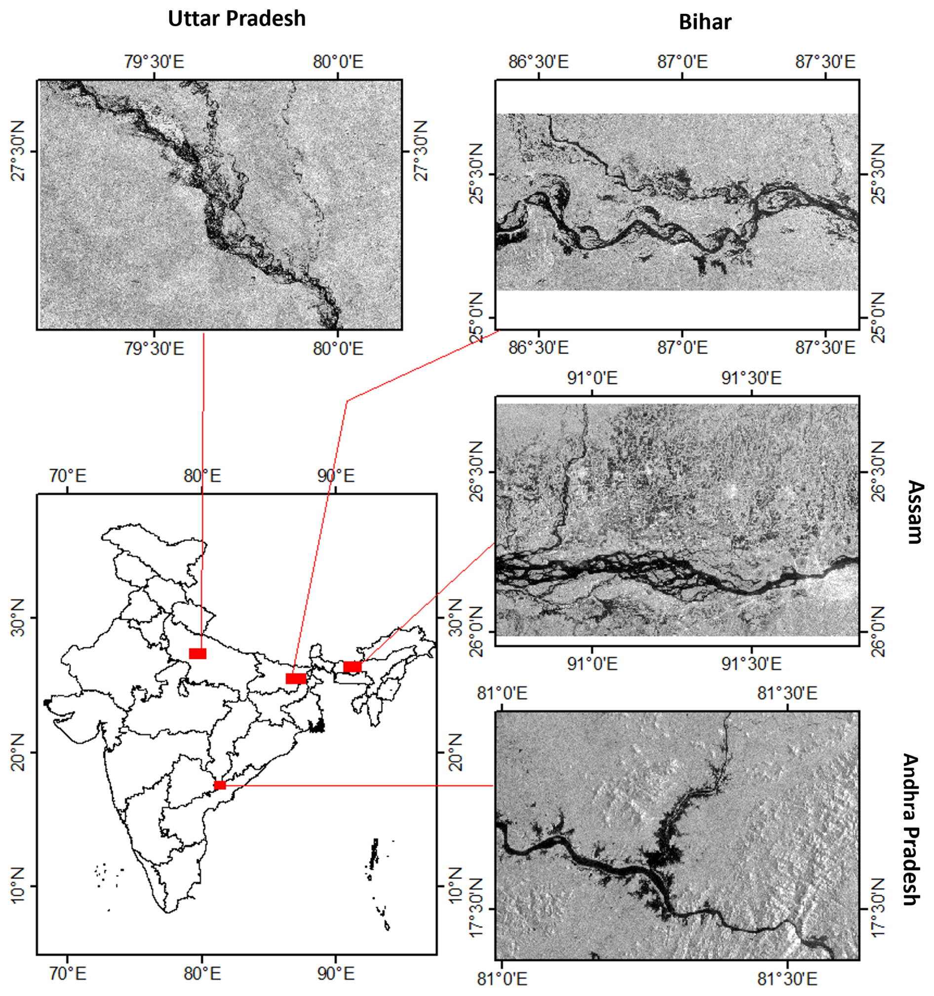
Figure 1 Publisher's remark: please note that the above figure contains disputed territories. Map showing four study area locations: Andhra Pradesh, Assam, Bihar, and Uttar Pradesh.

3 Data used

Comprehensive details regarding the satellite data and the associated digital elevation model (DEM) utilized for estimating flood inundation and depth are provided in Table 2. To validate the flood extent layers, optical datasets were employed, with additional specifics outlined in Table 3. Figure 2 illustrates the locations of river gauge stations and the field-measured water levels provided by the Central Water Commission (CWC) of India. In Fig. 2, permanent water bodies within each study area are clearly highlighted in blue.

Table 2 Satellite data and the DEMs used for the flood extent and depth estimation.

Table 3 Optical data used for the validation of flood extent.

3.1 Satellite data and digital elevation models

The Earth Observation Satellite 4 (EOS-04) is a synthetic aperture radar (SAR) satellite operating in the C-band frequency range of 5.4 GHz. Positioned in a sun-synchronous orbit at an altitude of 524.87 km, it offers various imaging modes, including fine-resolution strip mode (FRS), medium-resolution scanSAR mode (MRS), coarse-resolution scanSAR mode (CRS), and high-resolution spotlight mode (HRS). These modes allow the satellite to capture data with different levels of detail and coverage. The resolution ability of EOS-04 ranges from 1 to 50 m, enabling data acquisition at various spatial resolutions.

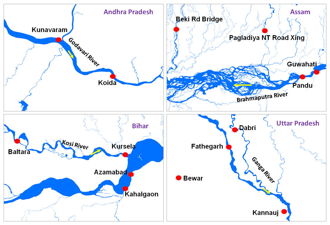
Figure 2 River gauge station locations in Andhra Pradesh, Assam, Bihar, and Uttar Pradesh. Note that the blue colour represents permanent water bodies in each study area.

3.2 Field measurements

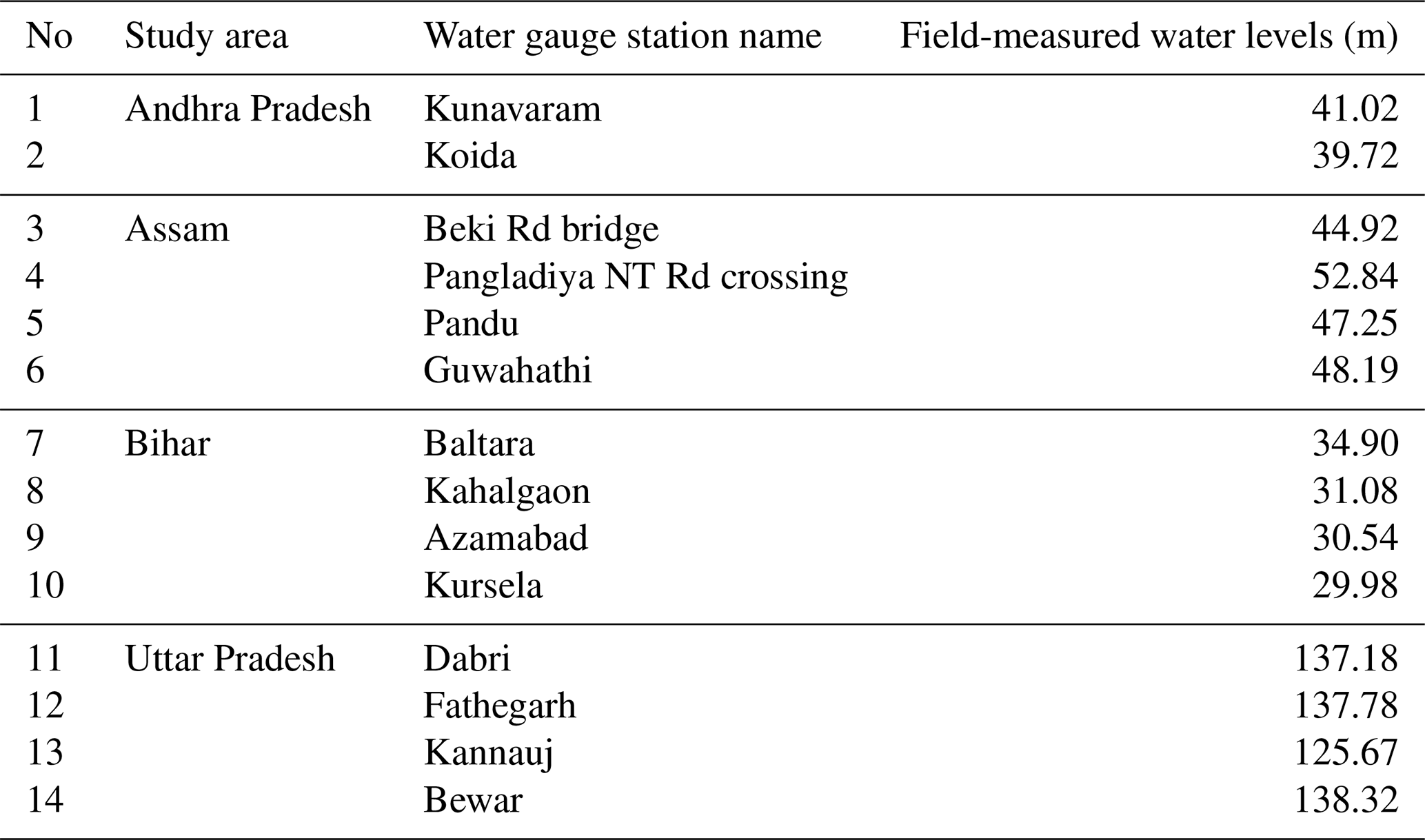
Typically, water levels are measured using gauge stations installed along rivers. The Central Water Commission (CWC) of India provides hourly field measurements from these gauge stations, as illustrated in Fig. 2 for various sites, and makes the information available on their website (https://ffs.india-water.gov.in/, last access: 11 July 2025). Water levels recorded at the times corresponding to satellite acquisitions across all study areas are compared with the interpolated levels derived from the trend surface analysis (TSA). Table 3 presents the field-measured water levels from gauge stations corresponding to the specific dates and times of satellite acquisitions.

Table 4 Field-measured water levels from gauge stations in the study area.

4 Methodology

The process of quickly estimating flood depth using the digital elevation model and EOS-04 imagery involves several steps. These include generating a radar backscatter coefficient image from the raw satellite image, extracting the flood inundation layer using an automated tile-based segmentation method, obtaining terrain information prior to the flood event using a digital elevation model, interpolating floodwater surface levels through trend surface analysis, and determining the spatial flood depth. The methodology is illustrated in the flow chart shown in Fig. 3a and b. Customized Python code has been developed specifically for automated flood mapping and depth estimation using the ArcGIS and GDAL libraries.

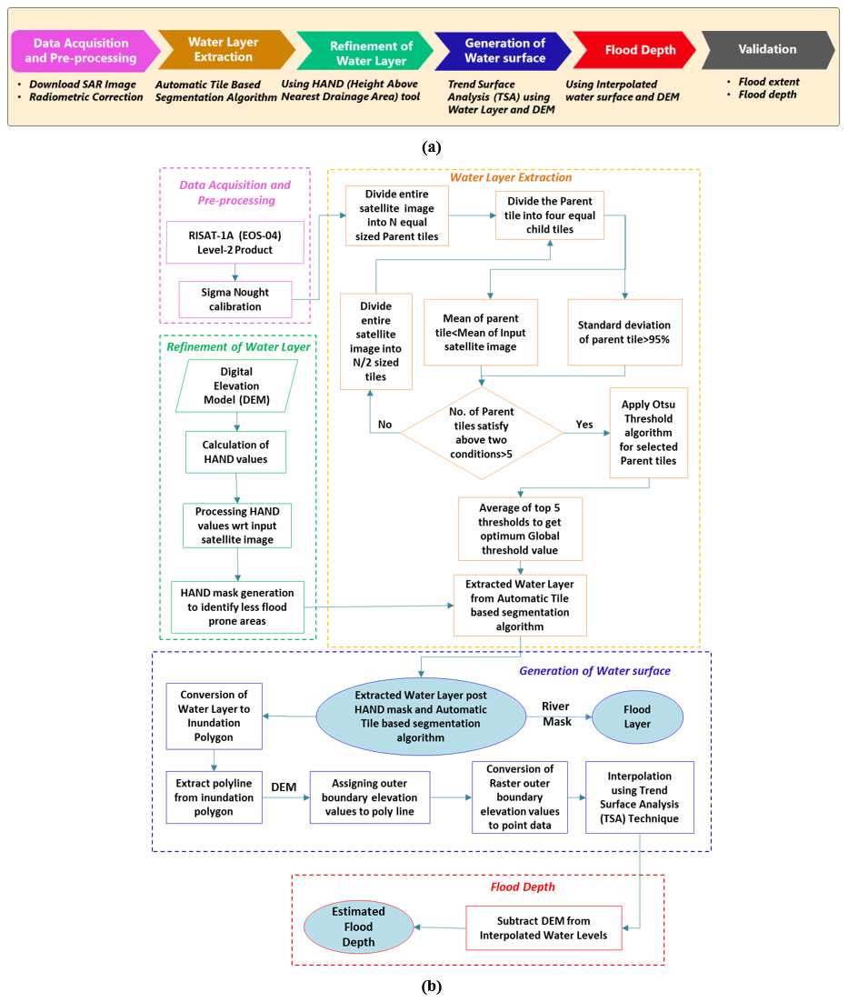
Figure 3 Methodology overview: (a) steps in the methodology and (b) a detailed flowchart illustrating the methodology.

4.1 Data acquisition and preprocessing

Any multi-sensor satellite data that are acquired after the flood event by satellite are hosted in the Indian Space Research Organization (ISRO)'s Bhoonidhi portal and can be downloaded. Preprocessing of EOS-04 data involves both geometric and radiometric corrections before the application of data for flood extraction (A. V. Suresh Babu et al., 2024). Geometric correction ensures the spatial accuracy of the SAR data by aligning it with a coordinate system or by correcting distortions caused by sensor geometry, Earth's curvature, and terrain variations. Radiometric correction involves adjusting the pixel values in the SAR data to accurately reflect the actual backscattered signal (converts raw digital numbers (DNs) into physical quantities such as backscatter intensity), compensating for system and environmental effects. This ensures consistency across sensors and acquisition times. Radar backscatter represents the intensity of the radar signal reflected back to the sensor from the Earth's surface, providing valuable insights into surface roughness, moisture content, and material properties. By analysing radar backscatter, water bodies can be accurately identified, surface conditions can be properly assessed, and land and water classification can be improved in remote sensing applications. Radar backscatter coefficient values, i.e. sigma nought (σ_o), for the EOS-04 image are computed using the following equation (Eq. (1)):

$$\begin{array}{}\text{(1)}& {\mathit{\sigma }}_o\left(\mathrm{dB}\right)=\mathrm{20}\times {\log }_{\mathrm{10}}\left(\mathrm{DN}\right)+\mathrm{10}\times {\log }_{\mathrm{10}}\sin {\mathit{\theta }}_{\mathrm{inc}}-\mathrm{CF},\end{array}$$

where DN represents the digital number (amplitude in level-2 products), θ_inc is the per-pixel local incidence angle, and CF is the calibration factor.

4.2 Water layer extraction

The water layer from the radiometrically calibrated image is extracted using the automatic-tile-based segmentation method, which involves partitioning the image into tiles and specific criteria-based tile selection, calculating thresholds, and classifying the image into water and non-water areas (Martinis et al., 2015), as illustrated in Fig. 4. The image is partitioned into non-overlapping tiles of equal size (n×n pixels), referred to as parent tiles. If perfect partitioning is not possible, the last row and column tiles are adjusted to ensure that they remain n×n pixels. Each parent tile is then subdivided into four equal-sized child tiles. For threshold calculation, tiles are selected based on two conditions.

1. The mean radar backscatter value of the parent tile should be lower than the mean backscatter value of the entire image, ensuring that the tiles are located near the boundary between water and non-water areas.

2. The standard deviation of the parent tile must exceed 95 % of the image's overall standard deviation, indicating significant variation within the tile, which enhances the classification of water and non-water areas.

If parent tiles that meet the specified conditions are less than 5 % of the total tiles, the image is subdivided into smaller tiles ($n/\mathrm{2}\times n/\mathrm{2}$), the standard deviation threshold is then relaxed to 90 %, and the process is repeated until the selected tile is sufficient. Once the necessary tiles are chosen, all parent tiles that satisfy both conditions are processed using the Otsu thresholding technique. The global threshold value is calculated as the average of the individual thresholds from the selected tiles and is used to classify the SAR image into water and non-water areas. This methodology is summarized in the flowchart presented in Fig. 3b.

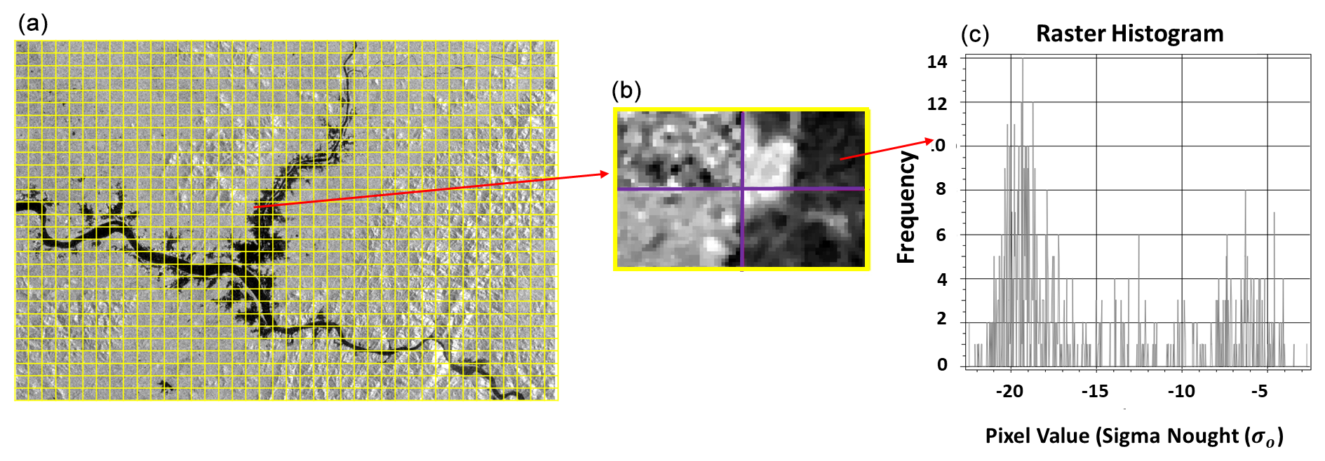
Figure 4 Automatic-tile-based segmentation of the SAR image. (a) Division of the SAR image into n parent tiles. (b) Division of the parent tile into four child tiles. (c) Histogram of one child tile.

4.3 Refinement of the water layer

To improve the accuracy of water classification and eliminate false water areas such as shadows and stray pixels caused by speckle noise, the height above nearest drainage (HAND) tool is employed. HAND is a terrain model that standardizes topography relative to the drainage network and characterizes local drainage potential. In a HAND raster, each pixel represents the vertical distance (in m) from that point to the nearest drainage channel. The HAND tool facilitates the rapid identification of non-flooded areas by restricting the flood areas up to a HAND value of 15 m, following the local drainage direction toward the channel where water flows. According to Nobre et al. (2015), regions with HAND values greater than 15 m are less vulnerable to flooding. Thus, applying the HAND mask refines the water layer, significantly reducing misclassification and subsequently producing the flood layer by subtracting a permanent river mask. The creation of a HAND raster from a DEM involves several steps, illustrated in Fig. 3b. These steps include the following:

• generating a seamless, hydrologically corrected DEM using the fill tool,

• defining flow paths using the flow direction function,

• identifying the drainage network through flow accumulation,

• calculating the HAND values using the D8 (eight-connectivity) flow distance algorithm.

4.4 Generation of the water surface

To estimate flood depth, it is necessary to generate a water surface using only a 2D inundated water layer and a digital elevation model (DEM) as input data with trend surface analysis (TSA). The TSA-generated water surface offers a notable advantage over traditional hydrodynamic models, which are often data-intensive. This streamlined approach provides a simplified yet effective solution for flood depth estimation. Trend surface analysis uses global polynomial interpolation to generate a smooth surface defined by a mathematical function derived from input sample points. This technique effectively captures gradual changes and coarse-scale patterns in the data, producing a smooth surface that reflects the overall trend across the area of interest (Morton and Pennycuick, 1974). TSA achieves this by fitting a polynomial function to known data points (outer-boundary elevation points) and using this function to predict values at locations where data are unavailable inside the flood extent. In this study, the outer-boundary elevation values derived from the DEM for the inundated water layer are used as input for the interpolation process. Based on the findings of Cohen et al. (2017), Huang et al. (2014), Brown et al. (2016), and Cian et al. (2018), it is assumed that the water surface in flooded areas is flat when calculating flood depth. In natural flood scenarios, water does not flow in abrupt steps like it would over steep or terraced terrain. Instead, floodwaters tend to spread out smoothly, forming a surface with a gentle slope or remaining nearly flat across large areas. This occurs because floodwater follows the path of least resistance, gradually filling depressions and expanding outward rather than forming sharp elevation differences. Given this characteristic, using a first-degree polynomial equation in the trend surface analysis (TSA) is a rational approach for modelling the floodwater surface. A first-degree polynomial represents a linear trend, which effectively captures the gradual variation in water surface elevation across the flooded area. This ensures that the estimated water surface reflects the actual spread of floodwater rather than introducing artificial discontinuities that would arise if higher-degree polynomials or abrupt elevation changes were assumed. By implementing this method, the study enhances flood depth estimation accuracy, as it aligns with the natural behaviour of floodwaters. The approach provides a more realistic representation of inundation, ensuring that calculated flood depths are consistent with the actual hydrodynamic conditions observed during flooding events.

Mathematically, the elevation observed at any point along the outer boundary of the inundated water surface can be expressed as the sum of the predicted elevation from TSA and the residual error at that point:

$$Z_{\mathrm{observed}}=f\left(x_i,y_i\right)+r_i.$$

Z_observed is the observed elevation value at the ith point inside the water surface, and f(x_i,y_i) is the polynomial function that predicts the elevation based on the coordinates x_i (latitude) and y_i(longitude). r_i represents the residual at the ith point, which is the difference between the observed and predicted elevations.

The first-degree polynomial equation used in this study is defined as follows :

$$f\left(x_i,y_i\right)=a{x}_i+b{y}_i+c,$$

where a, b, and c are constants that define the coefficients of the polynomial.

In real-world topographic surfaces, observed elevations rarely align perfectly with the predicted trend. Residuals r_i quantify the discrepancy:

• a positive residual indicates that the observed elevation is above the trend surface

• a negative residual indicates that the observed elevation is below the trend surface.

To determine the optimal coefficients a, b, and c, the least-squares criterion is employed, minimizing the sum of squared residuals (S):

$$S={\sum }_{i=\mathrm{1}}^N\left(r_i^{\mathrm{2}}\right),$$

where S represents the sum of squared residuals and r_i is the residual at the ith point.

The process used to derive the TSA-interpolated surface is illustrated in Fig. 5. First, the 2D water layer, obtained from the automatic-tile-based segmentation method, and the HAND tool, as shown in Fig. 5a, need to be converted into polygon form. This layer is then transformed into a polygon that retains only the outer-boundary segments. Next, the polygon is converted into raster format, and the corresponding outer-boundary elevation values are assigned from the digital elevation model (DEM). Since the TSA technique operates exclusively on point data, the raster is then converted to point form, as depicted in Fig. 5b. A first-degree polynomial surface is fit to the outer-boundary elevation values.

Predicted elevations are computed across the inundated area, producing an interpolated TSA water surface, as illustrated in Fig. 5c. The resulting TSA interpolated surface provides estimated water surface levels in metres.

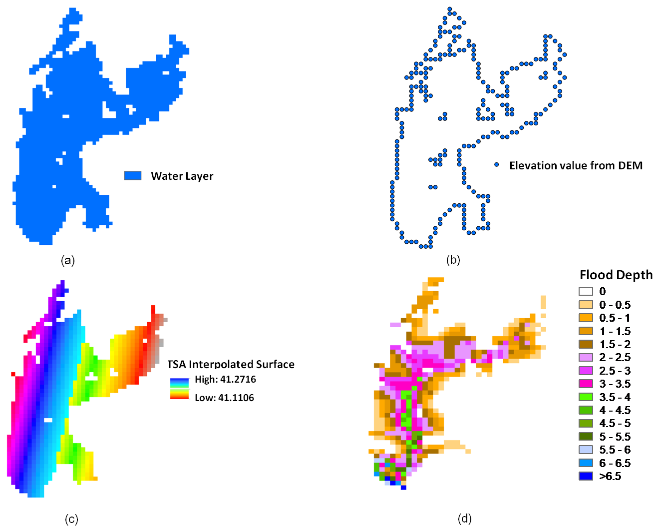
Figure 5 Methodology for flood depth estimation using the TSA technique. (a) The water layer is created using the automatic-tile-based segmentation technique and the HAND tool. (b) Elevation values are extracted as points for the outer-boundary water layer from the digital elevation model (DEM). (c) The interpolated surface is generated using these elevation points through trend surface analysis (TSA). (d) Flood depth is estimated by subtracting DEM values from the interpolated water levels (above mean sea level).

4.5 Flood depth

The calculation of flood depth is achieved by subtracting the digital elevation model (DEM) from the water levels interpolated by the TSA. The resulting depth is expressed in metres, as depicted in Fig. 5d.

5 Results

This research focuses on automated rapid flood inundation and depth estimation using synthetic aperture radar (SAR) imagery (EOS-04 data); the integration of the automatic-tile-based segmentation method and the height above nearest drainage (HAND) tool is validated for flood extent against cloud-free optical satellite data for Bihar and Uttar Pradesh, as detailed in Sect. 5.1. Floodwater depth is estimated in all study areas and validated according to Sect. 5.2. Accurate digital elevation models (DEMs) are critical for determining floodwater depth, but highly accurate DEMs are not available in all places; hence the assessment of the sensitivity of flood depth against DEM characteristics is required. This study uses a high-resolution 5 m lidar DEM and the 30 m Copernicus FAB-DEM for the Godavari River to assess flood depth sensitivity, as described in Sect. 5.2.1. Flood depth estimation using trend surface analysis (TSA) is conducted for the Godavari, Ganga, Brahmaputra, and Kosi rivers. The accuracy of TSA-derived flood depth estimates is assessed by comparing them with field-measured river water levels recorded by the Central Water Commission (CWC) for corresponding dates and times. Additionally, further comparisons with the floodwater depth estimation tool (FwDET) are comprehensively detailed in Sect. 5.2.2.

5.1 Flood inundation area estimation and validation

The flood inundation layer is created using the proposed method from EOS-04 data. Conducting fieldwork for flood map validation during a flood disaster is often challenging. Therefore, the accuracy of the delineated flood layer is assessed using a cloud-free optical satellite image from Landsat-8 at a 15 m resolution, which was acquired on the same date, i.e. 15 August 2023, as the EOS-04 data at an 18 m resolution in the Uttar Pradesh study area. Additionally, a Resourcesat-2 LISS-4 image at a 5.8 m resolution, also obtained on the same date as the EOS-04 image, i.e. 3 September 2023, was used for the Bihar study area. To extract water extent from the optical images, standard unsupervised classification techniques were applied using ERDAS Imagine software (Ali and Ansar, 2017). The results of this analysis are presented in Fig. 6, as shown below. Delineated flood pixels are shown in blue.

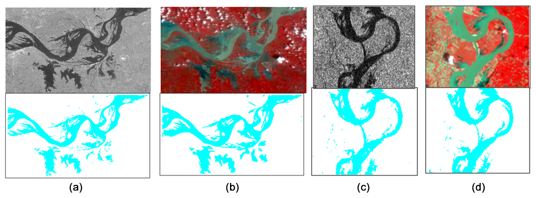
Figure 6 Comparison of optical satellite data and EOS-04 data. (a) EOS-04 data and the delineated flood layer using the automatic-tile-based segmentation method and the HAND tool in the Bihar study area. (b) Resourcesat-2 LISS-4 data and the flood inundation layer extracted using unsupervised classification in the Bihar study area. (c) EOS-04 data and the delineated flood layer using the automatic-tile-based segmentation method and the HAND tool in the Uttar Pradesh study area. (d) LANDSAT-8 data and the flood inundation layer extracted using unsupervised classification in the Uttar Pradesh study area.

As a part of the accuracy test for flood extent using the proposed method, the confusion matrix and performance metrics are computed for the Bihar and Uttar Pradesh study area using the respective optical datasets, as detailed in Tables 5 and 6.

Table 5 Confusion matrix for flooded and non-flooded pixels in Bihar and Uttar Pradesh study areas.

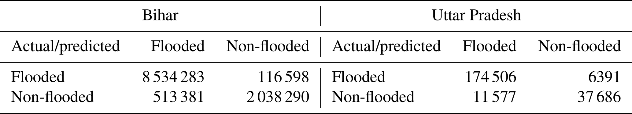
Table 6 Performance metrics for the flooded pixels in the Bihar and Uttar Pradesh study areas.

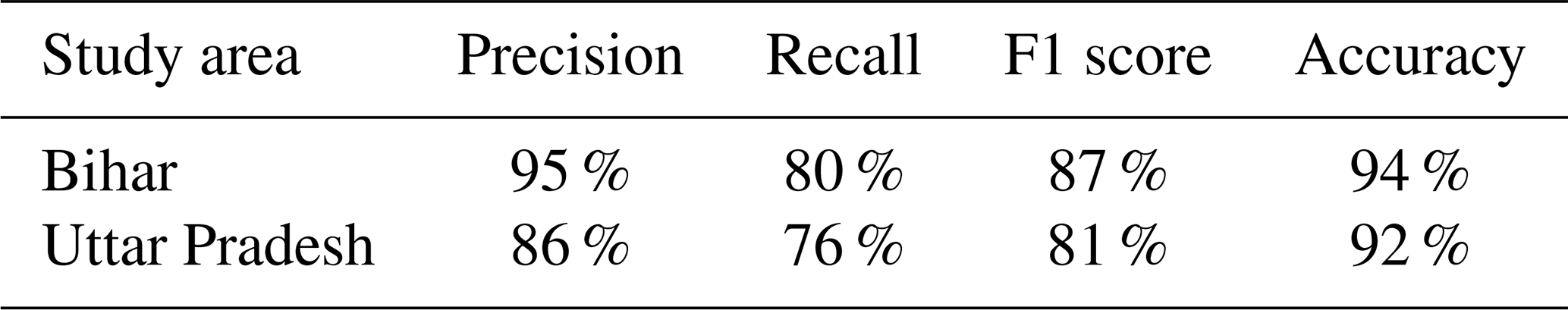
The flood delineation accuracy for the Bihar and Uttar Pradesh study areas exceeds 90 % when compared to the optical data in Table 6. However, certain discrepancies are observed when compared to Table 5 due to the characteristics of microwave data. In shallow flowing water areas, microwave sensors may incorrectly classify these regions as dry, unlike optical data, which accurately identifies the presence of water. Additionally, microwave data sometimes misinterpret moisture-laden areas as flooded, leading to overestimation.

Despite these limitations, the automatic-tile-based segmentation method combined with the HAND tool proves effective for generating flood maps rapidly using EOS-04 data. Since flood depth estimation relies on the delineated flood extent from SAR images, this method offers a reliable approach to automatically detect water layers, enabling efficient and accurate flood mapping in critical situations.

5.2 Floodwater depth estimation and validation

5.2.1 Sensitivity of flood depth with DEM characteristics

The accuracy of floodwater depth measurements depends significantly on the accuracy and spatial resolution of the digital elevation model (DEM), as it plays a major role in the interpolation of floodwater depth. To assess this, an analysis was conducted in the Godavari flood plain area utilizing two different DEM datasets. One DEM was derived from lidar data with a 5 m spatial resolution and a vertical accuracy of 15 cm, while the other was obtained from the public domain, specifically the Copernicus FAB-DEM, with an 8 m vertical accuracy and a 30 m spatial resolution. This comparative study aims to evaluate the impact of public domain DEMs on the accuracy of floodwater depth estimation. Here, the flood depth is estimated in the Godavari flood plain study area using the trend surface analysis (TSA) technique. The results of this analysis are presented in the Fig. 7 below. A scatter plot is drawn to compare flood depth values estimated using the TSA technique for lidar and Copernicus DEMs.

Figure 7 Plot between lidar-DEM-derived and Copernicus-DEM-derived flood depths.

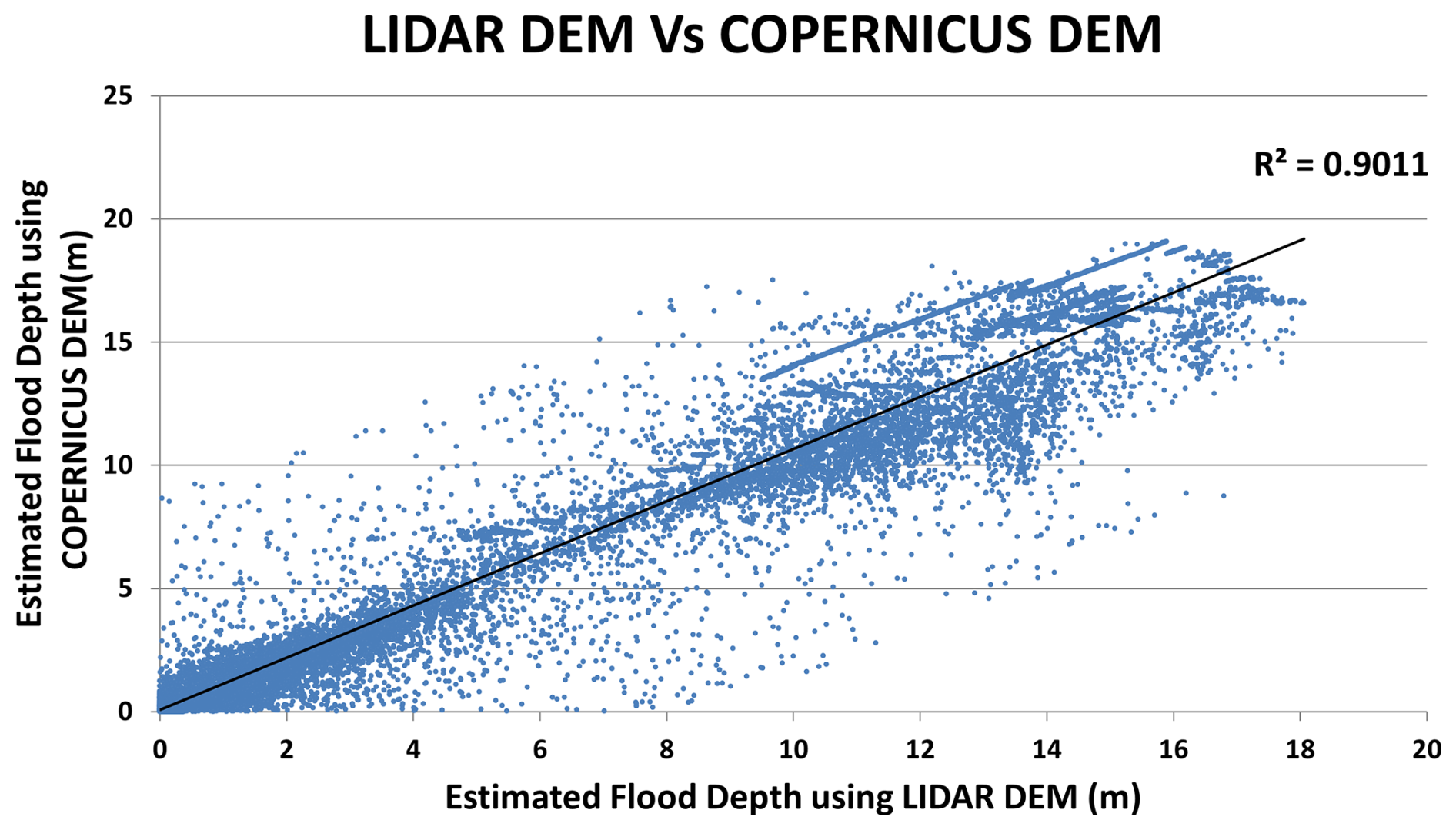
The scatter plot above indicates that 90 % of flood depth points derived from lidar and Copernicus DEMs match closely. The areas where discrepancies occur are predominantly in steep-slope regions where the elevation changes rapidly. Therefore, accurate lidar-derived DEMs are essential for estimating flood depths in steep areas. In contrast, for gentle-slope areas, Copernicus DEM with a 30 m spacing and vertical accuracy of 8 m provides sufficiently accurate flood depth estimates, as the depths are relative heights.

5.2.2 Results of the flood depth estimation and validation

The shape of flood layers varies across different areas, with some regions appearing wide, indicating a gentle slope, and others being narrow along rivers, suggesting a steeper gradient, as observed in the aforementioned case studies. There is an increasing demand for the accurate determination of flowing water surfaces to precisely estimate flood depths. Typically, the flowing water surface is derived through two steps: firstly, by collecting elevations along the flood inundation boundary, which represent varying heights of discrete points, and secondly, by fitting a surface across these elevation points using the proposed interpolation methods.

Derivation of flood depths using the TSA technique in the study areas

Given the dynamic nature of varying water levels of flowing rivers at different locations, employing trend surface analysis becomes essential to simulate the exact water surface, especially in large flooded areas with gentle slopes. This process involves calculating floodwater depths based on the DEM resolution at specific locations, such as pixels. Figure 8 below illustrates the flood depths in four areas of gentle slope. For the Andhra Pradesh study area, lidar-DEM-derived floodwater depth using TSA is illustrated in Fig. 8a. For the remaining three study areas, Bihar, Assam, and Uttar Pradesh, the publicly available Copernicus DEM is used to estimate floodwater depth using the TSA technique.

From Fig. 8, it is evident that the flood depth is greater in river areas, and it is represented in blue. Flood depths derived from the TSA technique are smooth and continuous.

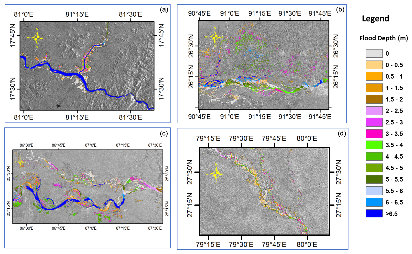
Figure 8 Flood depths calibrated using the TSA technique for the states of (a) Andhra Pradesh, (b) Assam, (c) Bihar, and (d) Uttar Pradesh.

Validation of flood depth results

The water levels derived using the trend surface analysis (TSA) technique in four case study areas are compared with field-based water level measurements from gauge stations provided by the Central Water Commission (CWC) for the same date and time. Figure 9 illustrates the method used to compare the TSA-derived water levels and the field measurements.

At each CWC river gauge station, TSA-interpolated water levels were computed. The field-measured water levels at the corresponding location, date, and time served as reference points for the comparison study. Table 7 presents the comparison results and also includes a comparison against water levels estimated using the floodwater depth estimation (FwDET) method. The FwDET water level estimations were performed in the open-source QGIS environment using the same study area's inundation water layer and a digital elevation model (DEM) as inputs.

Figure 9 Pictorial representation of the flood plain and river gauge station.

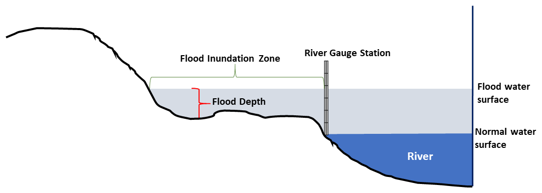
Table 7 Comparison study of water levels between field measurements, TSA, and FwDET.

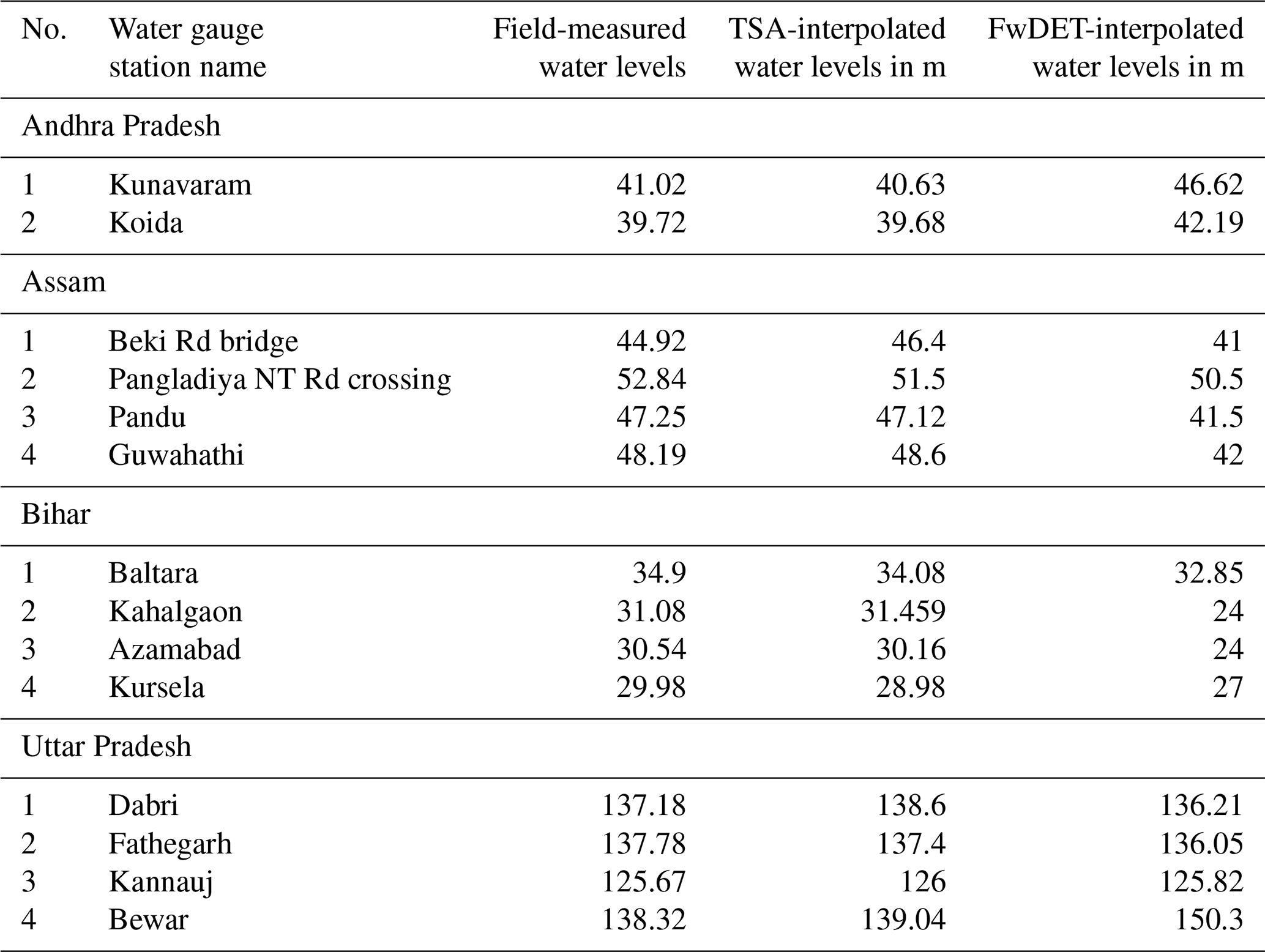
The results of the floodwater surface derived from surface trend analysis and the floodwater depth estimation tool (FwDET) indicate that the water surface from the trend analysis closely matches the water surface measurement at CWC gauge stations, whereas the surface derived from the FwDET tool shows significant deviations. TSA estimates deviate from field-level floodwater depth measurements by less than 65 cm on average across 14 gauge stations. Most interpolated water levels show a small difference (less than 50 cm) compared to field measurements. The underestimation of water levels by the TSA method is primarily due to the presence of real-time gauge stations on upstream flood plains. Conversely, overestimation occurs in areas where gauge stations are located on downstream flood plains.

The trend surface analysis method provides a more balanced and accurate representation of flood surfaces in such cases. However, it is observed that the slope of the flood-affected area plays a significant role in the accuracy of flood depth estimation. For gentle slopes, the accuracy of the TSA method is notably higher. Graphs are plotted in Fig. 10 for the case studies against river gauge station water level and field measurement and the TSA and FwDET methods.

In all case studies, the trend surface analysis (TSA) method outperforms the FwDET method when compared to field measurements. The root-mean-square error (RMSE) was calculated for both techniques, with TSA yielding an RMSE of 0.805, whereas FwDET produced an RMSE of 5.23. FwDET estimates generally exhibit sharp transitions in flood depth, while TSA provides a smoother depth distribution. Since the TSA-estimated depths also depend on the accuracy of flood extent mapping, the results indicate that the flood maps generated through the automatic-tile-based segmentation method appear to be accurate. The turnaround time for this entire process; i.e. flood mapping and flood depth, takes around 2 to 5 min on a desktop computer (3.2 GHz processor and 128 GB RAM) depending on the area of the case study.

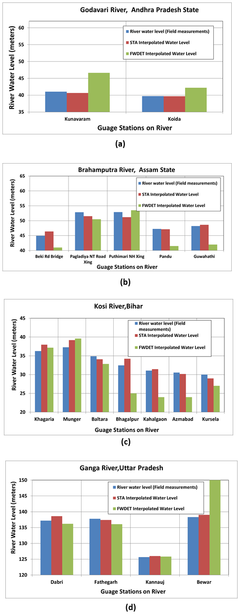
Figure 10 Comparison plots for water levels among field measured data, TSA, and FwDET for all study areas.

5.3 Discussion

This study introduces a novel approach framework for the rapid estimation of flood extent and depth using data from EOS-04, marking the first integration of such a methodology. The proposed method enhances the process of deriving flood extent compared to the automatic-tile-based threshold technique proposed by Martinis et al. (2015). While the tiling and tile selection criteria remain consistent with the earlier approach, the application of the thresholding technique is a key differentiator. Specifically, we employed the Otsu thresholding method in this paper instead of the minimum error thresholding method proposed by Kittler and Illingworth (1986). The minimum error thresholding method determines an optimal threshold by modelling pixel intensity distributions as two Gaussian distributions and by minimizing the probability of a classification error. This method is effective for images where pixel intensities follow a Gaussian distribution; it may not always be optimal where intensity distributions are complex. In contrast, Otsu's method, which maximizes between-class variance, is computationally efficient and more robust for the segmentation of flood extent in varying conditions. Thus, Otsu's approach was preferred in this study for its reliability in handling diverse flood scenarios. To further improve accuracy, we integrated the height above the nearest drainage (HAND) tool using digital elevation models (DEMs) to refine flood extent estimations. This enhancement addresses limitations in the earlier technique, offering a more topographically accurate representation of flood extent. Unlike Martinis's reliance on TerraSAR-X data operating in the X band, our approach utilizes data from EOS-04, which operates in the C band, demonstrating its applicability to a different radar frequency domain. However, the method has certain limitations; i.e. high-moisture areas are occasionally interpreted as flooded regions due to the radar's sensitivity to water content in soil. Furthermore, the method achieves optimal performance when the entire satellite scene is covered under the tile-fitting framework, ensuring comprehensive data representation.

The study also compares the trend surface analysis (TSA) method, a global fit interpolation technique, with local fit methods like the floodwater depth estimation tool (FwDET). TSA models the entire surface using global slope patterns, producing a smoother flood depth distribution that captures overall terrain slopes and gradients. This contrasts with FwDET, which interpolates at discrete points and often results in sharp depth transitions (Cohen et al., 2019). TSA produces a smoother distribution of flood depths, effectively capturing overall slope direction and gradients, as shown in Fig. 8. This makes TSA particularly adept at representing gradual terrain changes and mitigating noise or localized deviations, thereby providing a clearer understanding of flood dynamics over gentle slopes. Also, the TSA technique used in this study is not dependent on the watershed but rather on the slope and height of the terrain. The method relies on how water interacts with the landscape based on the terrain's incline, which directly influences the accuracy of flood depth estimation. When evaluating results against real-time field measurements using RMSEs, TSA consistently outperforms FwDET across all study areas. The lower RMSE of TSA indicates its superior accuracy when estimating flood depth compared to FwDET. A key advantage of TSA is that its efficiency is not constrained by the size of the study area; instead, the flood extent and hydrologically conditioned DEM play the most significant roles in its accuracy. In contrast, FwDET has predominantly been applied to smaller study areas in previous research, limiting its applicability to large-scale flood events. However, in real-world flood mapping, large flood extents are more common, making the scalability of an estimation method critical.

TSA has demonstrated superior performance in all aspects, providing more reliable flood depth estimations compared to FwDET. Its ability to adapt to different terrain and flood scenarios highlights its potential as a more effective and scalable approach for flood mapping applications.

TSA-derived flood depths were tested on both 5 m lidar DEM and the Copernicus 30 m DEM. The results, shown in Fig. 7, reveal a close match in depth estimates for areas with gentle slopes, demonstrating that even coarser DEMs, like the Copernicus 30 m DEM, can be effectively used for flood depth estimation in regions with gradual terrain. This broadens the applicability of the method to datasets with varying spatial resolutions. However, the methodology is sensitive to the DEM resolution and alignment with the flood layer, sometimes necessitating manual adjustments to ensure proper alignment between the DEM and flood extent.

While the method performs well in areas with gentle slopes, it has limitations in steep terrain where TSA may yield unreliable results. The TSA method fails to accurately represent flood depth in permanent water bodies and reservoir backwaters due to the lack of bathymetric data in DEMs, which only capture surface elevations. This can lead to underestimation or misinterpretation of flood depths, particularly in regions affected by backwater effects. Integrating bathymetric data or hydrodynamic models could significantly improve the accuracy of these estimations. Similarly, using hydrologically conditioned DEMs that account for artificial structures like bridges could also enhance accuracy.

A further challenge in validating flood depth estimates lies in the limited availability of field measurements, which are primarily taken near river gauge stations. This restricts validation to areas near main rivers, making it difficult to assess flood depths farther from these regions. Field measurements are also constrained by accessibility issues, limiting the ability to validate the model across the entire floodplain.

Although the methodology does not account for dynamic hydrodynamic characteristics such as flood velocity or temporal variations, the data generated through this approach are highly useful for real-time flood relief and rehabilitation efforts, particularly in rescue operations. The rapid and automated nature of this framework enables near-real-time flood assessment, supporting emergency response teams in deploying resources such as boats and skilled personnel more effectively. End users can confidently use this tool to plan mitigation strategies such as floodplain zoning and infrastructure protection, while recognizing its limitations when predicting dynamic flood behaviours, etc.

6 Conclusions

In summary, the integration of the automatic-tile-based segmentation method with the HAND (height above nearest drainage) tool, applied to EOS-04 data, has proven to be a highly effective approach to delineate flood layers. This method addresses key challenges, such as mitigating hill shadows and stray pixels in SAR data to eliminate false water classifications. The study also highlights the sensitivity of the publicly available DEMs, such as the Copernicus 30 m DEM, in regions with gentle slopes where high-resolution DEMs are unavailable. However, for steep flood-prone areas, fine-resolution DEMs remain essential to ensure accurate flood depth estimation.

The adoption of trend surface analysis (TSA) to interpolate water level data further enhances the accuracy and reliability of flood depth estimations, particularly in multidimensional river models. TSA effectively captures the spatial trends inherent in river systems, offering improved fitting and precise representations of flood surfaces. When combined, the automatic-tile-based segmentation and TSA techniques have demonstrated robustness and accuracy, as validated against field-measured data. Despite some limitations, this methodology enables rapid flood depth estimation across any flooded area using only a flood layer extent and a hydrologically conditioned DEM. The flood layer defines the inundation extent, while the conditioned DEM ensures accurate elevation representation. Without relying on complex hydrodynamic models or extensive field data, this approach allows quick and efficient flood assessment, making it valuable for emergency responses and large-scale flood mapping.

Future research will aim to test this methodology across diverse regions of the country to evaluate its broader applicability. Efforts will also focus on refining the approach to better accommodate varying terrain conditions, including steep slopes, and further improving the alignment and sensitivity of DEM-based flood depth estimations. However, there is a way forward: focusing on refining TSA to improve flood depth estimation in steep terrains, extending validation efforts using remote sensing data such as UAV-based lidar and Sentinel-3 altimetry, and integrating the proposed methodology into real-time flood monitoring systems to enhance disaster response and large-scale flood assessment.