Verifying the relationships among the variabilities of summer rainfall extremes over Japan in the d4PDF climate ensemble, Pacific sea surface temperature, and monsoon activity

Upper 99th percentile hourly, 90th percentile daily, and 90th percentile pentad rainfall values were calculated over the four largest Japanese islands for June–July every year in the 1952–2010 period, using 10 ensemble members of the 5 km resolution d4PDF (database for Policy Decision-making for Future climate changes) climate ensemble and 126 rain gauges. The HDBSCAN (Hierarchical Density-Based Spatial Clustering of Applications with Noise) algorithm was used to cluster rain gauges and d4PDF grid points, based on a multi-frequency metric. Six analysis regions were identified based on rain-gauge clusters. Spearman correlation was calculated between cluster rainfall extremes and standardised scores of five modes from the varimax-rotated extended principal component analysis of Pacific sea surface temperature (SST) anomalies. By order of explained variance for the analysis period, these modes represent El Niño–Southern Oscillation (ENSO) growth, ENSO decay, warming trend mixed with climate variability (Trend+), non-canonical ENSO, and other Pacific decadal variability (PDV). Rain gauges showed a field-significant correlation between hourly extremes and Trend+ and an anti-correlation between daily extremes and PDV; d4PDF showed excessive spatially widespread correlation and anti-correlation with ENSO decay and non-canonical ENSO, respectively. Rainfall extremes were better related to indices describing the regional monsoon jet's position and water vapour flux for both rain gauges and d4PDF. Modulation of the regional monsoon by the Pacific SST modes was used to explain the relationship between rainfall extremes and Pacific SST modes. The differences between rain gauges and d4PDF may be caused by slower monsoon development in d4PDF.

1 Introduction

Extreme rainfall events in recent summers have prompted the identification of regional conditions favourable to such developments (Harada et al., 2020; Yokoyama et al., 2020; Nayak and Takemi, 2021; Naka and Takemi, 2023). There is concern that climate change is increasing the strength of such events (Nayak and Takemi, 2019; Kamae et al., 2021; Mori et al., 2021) and there is interest in what spatio-temporal scales of rainfall are impacted (Fujibe, 2016; Unuma and Takemi, 2021). The authors wish to evaluate the changes of monsoon rainfall extremes (if any) in the future warmer climate; for this purpose, a standard procedure of calculating climate projections begins by comparing and verifying historical or control climate simulations with observations. The possible dependence of such extremes on internal climate variability complicates the calculation of climate projections, since climate variability itself may change in the future climate. Hence, in this study we evaluated the relationships between the variabilities of summer rainfall extremes over western Japan, monsoon activity, and Pacific sea surface temperature (SST).

Many hemisphere-scale modes of climate variability may interact with the regional- and global-scale signals over Japan; since Japan is an island located at the edge of the Pacific Ocean, it seems highly possible that the modes of Pacific SST have impacts on extreme rainfall over Japan. The dominant mode of Pacific SST variability is the El Niño–Southern Oscillation (ENSO). Although ENSO takes place in the tropical Pacific, it influences SSTs in the mid-latitudes and even globally in the form of the “Pacific-North America pattern” (Horel and Wallace, 1981; Hoskins and Karoly, 1981; see Alexander et al., 2002, for a literature review).

Over East Asia, the development of an El Niño during winter influences the following summer through the “Anomalous Philippine Sea Anti-cyclone”, persistent anti-cyclonic wind anomalies over the western North Pacific to the east of the Philippines which result in a wetter monsoon (e.g. Wang et al., 2000). The persistence of the El Niño signal has been explained by the “Indo–western Pacific Ocean Capacitor”, or teleconnections into and returning from the Indian Ocean (Kosaka et al., 2013; Xie et al., 2016), which excite a series of alternating high-and-low pressure, temperature, and convection systems across the region termed the “Pacific-Japan” (P–J) pattern (Nitta, 1987).

While the El Niño-associated anomalous anti-cyclone is one lobe of the P–J pattern, the P–J pattern is excited not only by ENSO. A positive Indian Ocean Dipole (IOD) occurring by itself without an El Niño would also have a teleconnection to the Pacific. An extremely warm Indian Ocean since 2019 likely contributed to the extreme rainfall event of 2020 (Takaya et al., 2020), in conjunction with other exacerbating factors like the Madden–Julian Oscillation (Zhang et al., 2021). The P–J pattern can also be excited by Rossby wave breaking (Takemura and Mukougawa, 2022), which increases during La Niña-like conditions in summer (Takemura et al., 2020). Such results suggest that it will be difficult to find clean and robust relationships between the ENSO phase and rainfall over Japan.

An early study using data for a 30-year period (1951–1980) found no evident relationship between the bai-u (monsoon front) rainfall and the Southern Oscillation Index (SOI) of the season (Ninomiya and Mizuno, 1987). A study using other 30-year (1963–1992) period data found that the relationship changed from bai-u rainfall lagging the Niño3 index during 1963–1977 to leading Niño3 during 1978–1992 (Tanaka, 1997). A study of rainfall in Fukuoka (on Kyushu island) for about a century (1890–2000) using categorised SOI found heavy rainfall to lag the “Strong La Niña” category (Kawamura et al., 2001; Jin et al., 2005). Yet another study for a period of 54 years (1958–2011) found that weather patterns associated with heavy rainfall over Japan occurred more frequently when the Niño3.4 index of the season was high (Ohba et al., 2015). Such examples suggest that the relationship between ENSO and rainfall over Japan may depend on the period of data or even the location being studied. ENSO has a period of about 5–7 years, so even a 100-year period would contain only about 20 cycles. A 400-year study using palaeoclimate proxies concluded that the strength and even sign of the relationship varied over time, and it proposed that the Pacific Decadal Oscillation modulated the relationship (Sakashita et al., 2016). It appears that the scientific literature is far from unanimous regarding the relationship between ENSO and rainfall variability over Japan.

Since we were unable to draw satisfactory conclusions from those past studies, we decided to investigate the relationships between Pacific climate variability and extreme rainfall variability in the monsoon season over Japan in observations first, before applying the same methodology to climate models. The methodology was based on two considerations.

Firstly, although the SOI or Niño indices indicate the ENSO-related state of the atmosphere and ocean, respectively, ENSO phases are not instantaneous states but processes that develop and decay over the course of 2 years, even though SOI/Niño indices may have similar values before and after the ENSO peak. Clearer relationships may emerge between rainfall and an indicator measuring the direction of ENSO progress.

Secondly, the value of SOI/Niño indices may reflect not only the ENSO state, but also the states of other modes, such as the above-mentioned Pacific Decadal Oscillation. This study will directly decompose Pacific SST anomalies through rotated extended principal component analysis (rePCA) and correlate between each mode and extreme rainfall, instead of using the SOI/Niño indices.

The structure of this paper is organised as follows. Section 2 describes the data and methods used. Section 3 describes the results from the of Pacific SST, rainfall clustering, and correlation of SST modes with clustered rainfall extremes. In Sect. 4, we discuss how the SST modes may act on rainfall through monsoon activity. Finally, Sect. 5 summarises the findings of the study.

2 Data and methods

2.1 Data and tools

2.1.1 Rainfall data

The “database for Policy Decision-making for Future climate changes” (d4PDF) is a collection of ensemble climate simulations covering the 1951–2010 period (Mizuta et al., 2017; Ishii and Mori, 2020). A 100-member historical-warming climate ensemble has been simulated by the Meteorological Research Institute (MRI) Atmospheric General Circulation Model (AGCM) version 3.2 (MRI-AGCM3.2; Mizuta et al., 2012), which provided rainfall at 60 km spatial and daily temporal resolution. Twelve members have been downscaled to 5 km spatial and hourly temporal resolutions (Kawase et al., 2023); d4PDF in this study will refer to the downscaled data, and the AGCM will be termed “d4PDF-AGCM”. Ensemble mean rainfall extremes from 10 members of the 5 km d4PDF were compared against rain-gauge rainfall extremes from 126 meteorological stations in Japan. The analysis period was 1952–2010 (or 59 years).

Rainfall during June and July was analysed. This is the season when the monsoon (bai-u) front passes over the study domain. An analysis of typhoon frequency was carried out for each month using the International Best Track Archive for Climate Stewardship (IBTrACS; Knapp et al., 2018) for observations and Webb et al. (2019) for d4PDF. The number of typhoons was found to increase substantially in August. Evaluating typhoon changes in the future climate is not trivial (see Mori and Takemi, 2016, for a review), so the authors preferred to exclude typhoon-associated rainfall as much as possible, even though the typical calendar summer includes August. From a phenomenon perspective, August rainfall over Japan is climatologically quite distinct from June–July rainfall. The 99th percentile hourly, 90th percentile daily, and 90th percentile running-pentad rainfall values in June–July of every year were calculated. Percentiles were calculated inclusive of time steps with no rainfall.

2.1.2 Sea surface temperature (SST) and climate mode indices

The historical d4PDF-AGCM ensemble was driven by randomly perturbed SST from the Centennial Observation-Based Estimates of SST version 2 (COBE-SST2; Hirahara et al., 2014). The SST data were of 1° spatial resolution and monthly temporal resolution. Data over the Pacific in the domain of 100° E–60° W and 20° S–60° N were used. Data on the Atlantic side were removed. Data over the Sea of Okhotsk (135–160° E, 45–60° N) were removed, in order to reduce the influence of sea ice. The same 59-year period as the rainfall period (1952–2010) was used for analysis, but it also included December 1951, January 2011, and February 2011.

The Southern Oscillation Index (SOI; Ropelewski and Jones, 1987) and Interdecadal Pacific Oscillation (IPO) Tripole Index (TPI; Henley et al., 2015) were provided by the United States of America National Oceanic and Atmospheric Administration (NOAA). The non-standardised version of the SOI was used, but standardisation has no impact on correlation. The filtered COBE-SST version of the TPI was used, with units of degrees Celsius (°C). The North Pacific Gyre Oscillation (NPGO; Di Lorenzo et al., 2008) index was used, available at https://o3d.org/npgo (last access: 27 June 2025).

2.1.3 Other meteorological variables

Meteorological variables in the region of 125–130° E and 20–50° N from the Japanese 55-year reanalysis (JRA55; Kobayashi et al., 2015) and d4PDF-AGCM were used to evaluate the monsoon activity. The datasets were obtained at 1.25° spatial resolution. The 850 hPa daily mean temperature and specific humidity were used to calculate the monsoon front location. Zonal wind, meridional wind, and specific humidity at pressure levels of 1000, 925, 850, 700, 600, and 500 hPa were used to calculate water vapour flux. Monsoon activity in the simulations was evaluated using variables from d4PDF-AGCM using the same 10 ensemble members as the rainfall data. The period of 1958–2022 was used because JRA55 started from 1958.

2.1.4 Processing tools

Coastlines and administrative boundaries were obtained from the Database of Global Administrative Areas version 4.1 (GADM; https://gadm.org, last access: 27 June 2025). Principal component analysis and part of the data processing was carried out using the Max Planck Institute for Meteorology's Climate Data Operators software package (CDO; Schulzweida, 2022). Equivalent potential temperature was calculated using the NCAR Command Language (NCL, 2019). The rest of the data processing was carried out in Python 3, using Python libraries NumPy (Harris et al., 2020), SciPy (Virtanen et al., 2020), pandas (McKinney, 2010), and xarray (Hoyer and Hamman, 2017). Clustering of rainfall and curve fitting were carried out using SciPy. Wavelet analysis was carried out using PyWavelets (Lee et al., 2019). Figures were prepared with the Python libraries Matplotlib (Hunter, 2007), Cartopy (Met Office, 2010–2015), and the GNU Image Manipulation Program (GIMP, 2025).

2.2 Method

2.2.1 Rotated extended principal component analysis (rePCA)

The SST field from COBE-SST2 was cropped to the domain of 100° E–60° W and 20° S–60° N. SST anomalies were calculated by subtracting the long-term monthly mean of the analysis period from the monthly SST, at each grid point. The anomalies were weighted by area with the cosine of latitude. Principal component analysis was performed on the concatenation of five seasonal mean anomalies, centred on the JJA season of the indexed year; i.e. the sample of 1952 would consist of D[−1]JF (December 1951, January 1952, February 1952), MAM (March 1952, April 1952, May 1952), JJA (March 1952, April 1952, May 1952), SON (September 1952, October 1952, November 1952), and DJ[+1]F[+1] (December 1952, January 1953, February 1953) seasonal mean anomalies. This is known as extended principal component analysis or a multichannel singular spectrum analysis with embedding dimension 5 and trimestral sampling. The anomalies were not standardised before PCA. Extended PCA has been used in past studies to obtain the time evolution patterns of Pacific SST anomaly modes (Weare and Nasstrom, 1982; Guan and Nigam, 2008).

After extended PCA, the weighting by area was removed. Standardised scores and loadings were calculated from the principal components (PCs) and empirical orthogonal functions (EOFs); i.e. each PC (EOF) was divided (multiplied) by the square root of its corresponding eigenvalue to give the score (loading), so the strength of the loading indicates its contribution to the total variance of temperature anomalies. A varimax rotation was performed on the 29 top modes, and the rotated modes were reordered by their explained variance. Twenty-nine modes were used for rotation following Guan and Nigam (2008), who selected this number based on the number of modes being above “noise level”.

COBE-SST2 was also compared with COBE-SST (Ishii et al., 2005; Japan Meteorological Agency, 2006), which produced similar climate modes except for the “Trend-including” mode (not shown). This mode was sensitive to the analysis time period, even for the same COBE-SST2 dataset, as will be described in Sect. 3.1 (Figs. 1 and 2), where rePCA was carried out for the 1921–2022 and 1952–2022 periods to examine the robustness of the resultant modes. The rePCA results used for comparison with rainfall were based on rePCA of the 1952–2010 period, i.e. the same period as the rainfall.

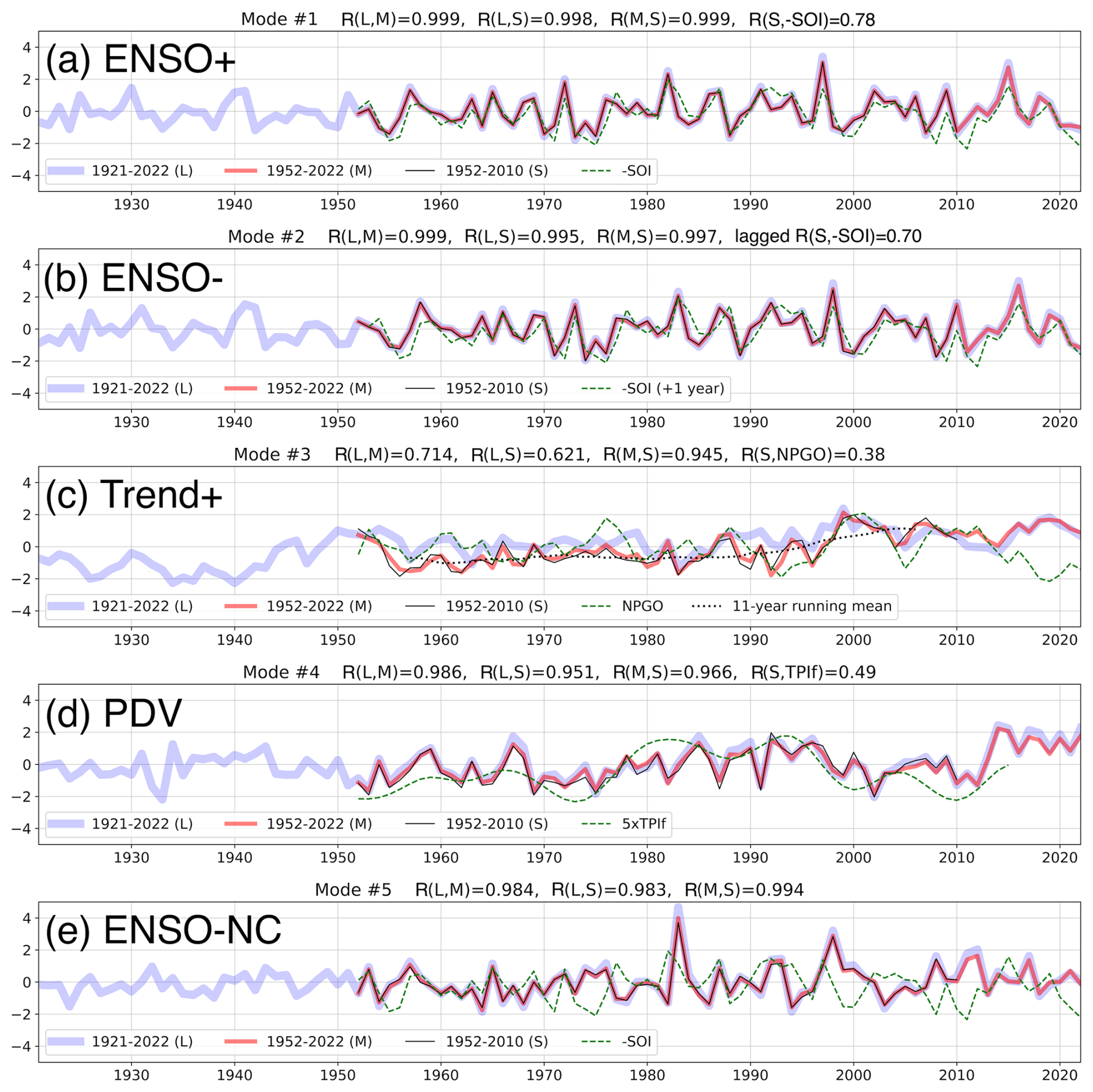
Figure 1 Standardised principal components (scores) of the first five modes from the rotated extended PCA of Pacific SST anomalies for years 1921–2022 (blue), 1952–2022 (red), and 1952–2010 (black). (a) Canonical ENSO-growth mode “ENSO+”; (b) canonical ENSO-decay mode “ENSO-”; (c) trend-containing mode “Trend+”; (d) Pacific decadal variability mode “PDV”; (e) non-canonical ENSO “ENSO-NC”. The dotted black line in panel (c) shows the 11-year running mean of the 1952–2010 score. The dashed green line in the panels shows (a) negative of the Southern Oscillation Index “-SOI”, (b) negative of the Southern Oscillation Index phase-shifted by 1 year “-SOI (+1 year)”, (c) North Pacific Gyre Oscillation index “NPGO”, (d) Interdecadal Pacific Oscillation Tripole Index filtered version “TPIf” (in °C scaled by a factor of 5), and (e) negative of the Southern Oscillation Index “-SOI”. The correlation coefficients between the scores from 1921–2022 “L”, 1952–2022 “M”, and 1952–2010 “S” for overlapping periods are shown on the top of the panels, as well as correlation coefficients between “S” scores and the green index for panels (a)–(d).

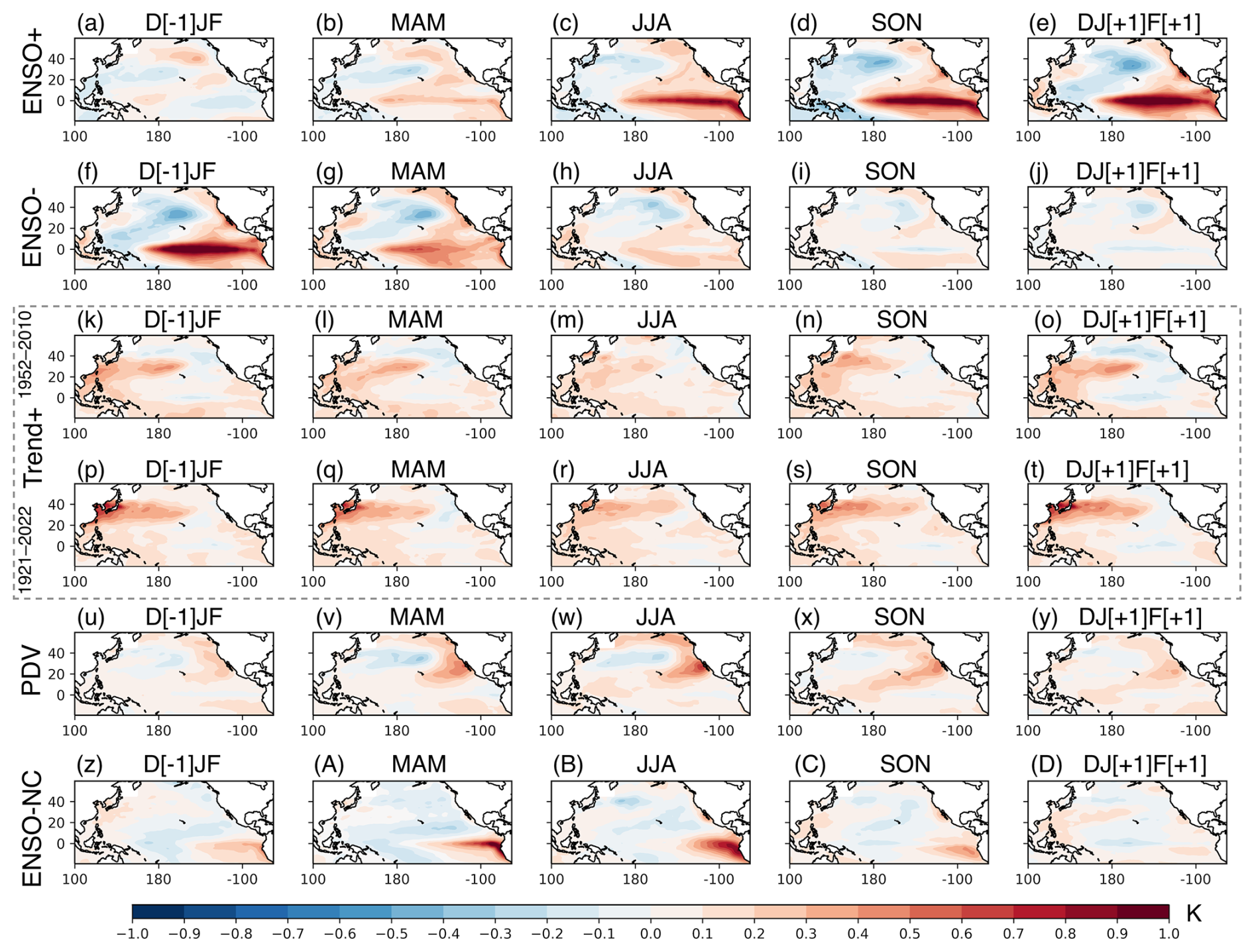
Figure 2 Loadings of the first five modes from the rotated extended PCA of Pacific SST anomalies for the 1952–2010 period and only the Trend+ mode for the 1921–2022 period. Rows show the modes. Row 1 (a–e) ENSO+; row 2 (f–j) ENSO-; row 3 (k–o) Trend+; row 4 (p–t) Trend+ for 1921–2022; row 5 (u–y) PDV; row 6 (z–D) ENSO-NC. Columns show anomalies of five seasons centred on June–July–August (JJA).

2.2.2 Rainfall clustering

Upper-percentile rainfall in June–July of every year was calculated for individual rain gauges, as well as individual grid points of d4PDF within a convex hull covering the four large Japanese islands of Hokkaido (northern diamond-shaped island), Honshu (S-shaped large island), Shikoku (southern barbell-shaped island), and Kyushu (southwestern oval-shaped island). The last 2 d of May and the first 2 d of August were used in the calculation of running pentads. The percentile calculation was inclusive of times with zero rainfall. For hourly rainfall, the 99th percentile was the 15th highest value of the June–July season. For daily and running-pentad rainfall, the 90th percentiles were the sixth-highest values. This produced time series of 59 samples (years). For d4PDF, percentiles were calculated for each individual ensemble member, then the ensemble mean was taken.

The hourly rainfall in June–July of every year at individual locations was also decomposed into different frequency components through projection onto wavelet space, using stationary (non-downsampled discrete) wavelet transform based on the Haar wavelet with six decomposition levels. A prior examination of the hourly data using continuous wavelet transformation on the rainfall indicated that most of the energy was within frequencies resolved by six discrete decomposition levels. This produced six detailed components with periods of 2–4 h (D1), 4–8 h (D2), 8–16 h (D3), 16 h–1.3 d (D4), 1.3–2.7 d (D5), 2.7–5.3 d (D6) and one approximation component containing signals of periods longer than 5.3 d (A6). The number of samples in each component remained the same since the input was not downsampled, so the 99th percentile of each June–July season was recorded for each component. Hence, the rainfall at each location was reduced to a 59×7 (year × frequency component) matrix. Wavelet transformation (Torrence and Compo, 1998) has been successfully used to analyse rainfall at the Matsuyama rain gauge (Santos et al., 2001) and precipitation indices over Japan (Duan et al., 2015), although for data of monthly resolution.

The spatial points were clustered using the Hierarchical Density-Based Spatial Clustering of Applications with Noise (HDBSCAN) function, SciPy's implementation of the hierarchical density-based clustering algorithm developed by Campello et al. (2013). This algorithm builds a hierarchical tree of the samples (points) by searching around the vicinity of each sample at increasing radius based on a distance metric (D), merging samples into increasingly larger clusters as they are found, then returning the most persistent clusters above a minimum cluster size (c_min) along the tree's depth. The tree-construction algorithm was set by the user to brute force (“brute”); i.e. the tree was explicitly constructed. The manner in which clusters grew to fulfil the requirement of increasing c_min depended on the minimum sample size, which was set to 1; i.e. even one sample that was significantly correlated with any member of the cluster would be added to the cluster, allowing the cluster to keep expanding until no more such samples could be found.

The distance metric between two points i and j was defined as $D=\mathrm{1}-r_{ij}$, where the geographically adjusted similarity $r_{ij}\in [-\mathrm{1},\mathrm{1}]$. For each clustering of points based on their hourly, daily, and running-pentad rainfall extremes,

$$\begin{array}{rl}& r_{ij}=\\ & \left\{\begin{array}{ll}-\mathrm{1}& \text{if}{R}_{ij}\text{is statistically significant}\\ & \text{and negative,}\\ \mathrm{0}& \text{if}{R}_{ij}\text{is not statistically}\\ & \text{significant,}\\ max(\mathrm{0},R_{ij}-s_{ij})& \text{if}{R}_{ij}\text{is statistically significant}\\ & \text{and positive,}\end{array}\right.\end{array}$$

using the Spearman correlation R_ij and geographical adjustment factor $s_{ij}=S_{ij}/S_{\text{max}}$. The Spearman correlation R_ij between the rainfall time series of points i and j was evaluated for statistical significance using a two-tailed test at α=0.05; i.e. significant if $\left|R_{ij}\right|>\mathrm{0.256}$ for the 59-sample (years) period of 1952–2010. The geographical adjustment s_ij is the physical distance between the two points S_ij normalised through division by a maximal distance S_max, which will be described later. This metric is similar to that used in the clustering by F madogram (Bernard et al., 2013) with geographical adjustment factor (Bracken et al., 2015), which has been successfully applied to the Tibetan Plateau (Ma et al., 2020), an orographically complex region similar to our study domain.

For clustering of points based on wavelet decomposition, there were multiple Spearman correlation coefficients $R_{ij}^k$ and their corresponding similarity values $r_{ij}^k$, for $k=\mathrm{0},\mathrm{\dots },n_k$, where n_k=6, representing the frequency components A6, D6, … , D1. In this case, r_ij was defined:

$$\begin{array}{rl}& r_{ij}=\\ & \left\{\begin{array}{ll}-\mathrm{1}& \text{if}{r}_{ij}^k\text{is negative for any}k,\\ max(\mathrm{0},{\sum }_k{r}_{ij}^k/n_k-s_{ij})& \text{otherwise,}\end{array}\right.\end{array}$$

where

$$r_{ij}^k=\left\{\begin{array}{ll}-\mathrm{1}& \text{if}{R}_{ij}^k\text{is statistically significant and negative,}\\ \mathrm{0}& \text{if}{R}_{ij}^k\text{is not statistically significant,}\\ R_{ij}^k& \text{if}{R}_{ij}^k\text{is statistically significant and positive.}\end{array}\right.$$

When n_k=1, this reduces to the version used in clustering hourly, daily, or running-pentad extremes. The maximum function in the calculation of r_ij implements a lower bound of zero in cases of significantly correlated distant points. At sufficiently large distances, r_ij would be attenuated to the case such that there were no statistically significant R values, or D=1. Both cases were distinct from the case where significant anti-correlation was found, where the points should not be clustered, and D=2. While the maximum function was not strictly necessary, it provided two advantages. Firstly, since c_min was a user-provided parameter, a method of selecting an optimal c_min was needed. When there was a step jump in D, we found that as the algorithm was iterated with increasing c_min, there was a change in the number of clusters when a certain c_min threshold was reached. A plateau was reached when the number of clusters remained the same. For d4PDF gridded data, this took the form of a singular cluster consisting of almost all grid points in the domain and a few tiny clusters over the Japanese Alps. Such a configuration was not interesting, so the previous c_min was selected. Secondly, by reducing r values to only indicate desirable to cluster (r>0) or strongly undesirable to cluster ($r=-\mathrm{1}$), most r values were zero. This allowed for efficient storage of r values as sparse matrices, which was particularly important for d4PDF with over 35 000 points.

To speed up the calculation, s_ij was approximated using degree distance for S_ij and 20° for S_max, the approximate degree distance from southwest to northeast of the d4PDF study region. Two points with minimally significant R of approximately 0.25 would only be completely attenuated when their geographical degree distance exceeded 5°, which was sufficiently generous when compared against the smaller geographical extent of clusters obtained from rain gauges. In the case of d4PDF, a further threshold S_calc was set, where r_ij was calculated only for pairs (i, j) where S_ij<S_calc. A token value of S_calc=1° was set based on the size of the rain-gauge clusters, and the results were checked against results obtained from halving and doubling S_calc.

The results using the wavelet-based distance metric were compared against results from individually clustering three temporal resolutions (hourly, daily, and running-pentad) for rain gauges, before being applied to d4PDF. The comparison method is described in the following section.

2.2.3 Selection of analysis regions

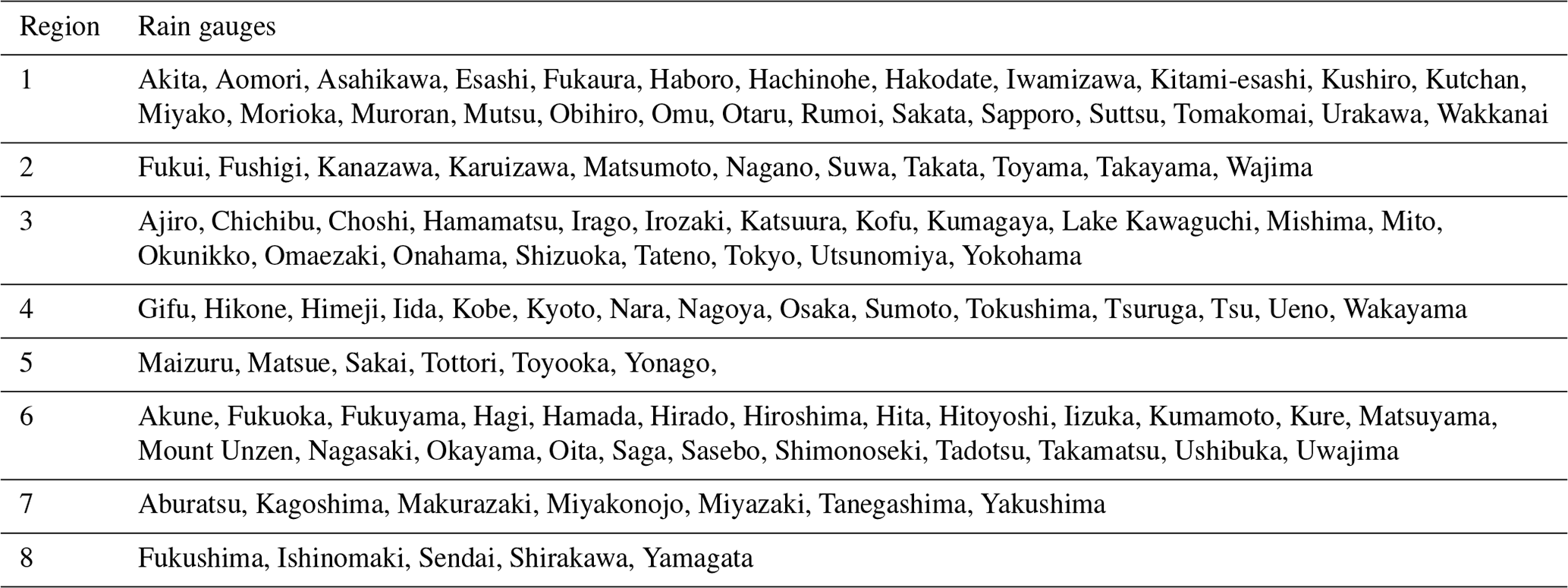
To combine the results of individually clustering hourly, daily, and running-pentad extremes, we would like to group the rain gauges into regions that persisted across the three temporal resolutions. The most suitable c_min among the three temporal resolutions was commonly applied to all three resolutions. Rain gauges belonging to the same set of clusters produced at three temporal resolutions were grouped together (“3Class”). To illustrate this, if $(A,B,C,D,E,F,G)$ was an hourly cluster, $(A,B,C)$ and $(E,F,G)$ were daily clusters, and $(A,B,D)$ and $(C,E,F,G)$ were pentad clusters, then the 3Class regions would be (A,B) and $(E,F,G)$. A 3Class group must contain at least two rain gauges. The 3Class regions were compared with the clusters produced by the wavelet-based distance metric, and eight regions were finally selected for analysis. These are listed in Table 1, and the comparison process will be described in Sect. 3.2.

Table 1 The eight regions selected for analysis and the rain gauges in Japan.

A time series of rainfall was calculated for each cluster or unclassified location, commonly referred to as sets. The mean rainfall of the set was calculated at every time step and was considered as one sample. The number of samples every year would hence remain the same between different sets for the calculation of percentile rainfall. Upper-percentile rainfall for each set was calculated every year from the set's rainfall time series.

When directly comparing regional values between rain gauges and d4PDF, statistics were calculated from d4PDF clusters co-located with the rain gauges of the region. A d4PDF cluster was considered co-located with the rain gauge if any grid point belonging to that cluster lay within 0.05° of the rain-gauge location.

2.2.4 Evaluation of correlation coefficients (R)

In this study, Spearman correlation was used, which measured only monotonicity between two variables without the need for linearity. The correlation coefficient R was tested for statistical significance using a two-tailed test at α=0.05. For the 59-year period of 1952–2010, the threshold value is $\left|R\right|=\mathrm{0.256}$. Analysis of JRA55 used the 53-year period of 1958–2010, with threshold value $\left|R\right|=\mathrm{0.270}$. In the text, R will be described as perfect if $\left|R\right|=\mathrm{1.00}$, strong if $\mathrm{1.00}>\left|R\right|\ge \mathrm{0.75}$, moderate if $\mathrm{0.75}>\left|R\right|\ge \mathrm{0.50}$, weak if $\mathrm{0.50}>\left|R\right|\ge \mathrm{0.25}$, and no relation otherwise.

When multiple significance tests are repeatedly performed, a number of false positives may occur. The number of positives must exceed a threshold for there to be statistical significance for the entire field, i.e. field significance. Rain-gauge R values were tested for field significance following the methodology of Livezey and Chen (1983). If individual rain gauges were considered independent samples, significance for at least 12 rain gauges would be required for field significance. If the eight analysis regions were used as samples (since the method requires samples to be mutually independent), significance for at least three regions would be required for field significance.

2.2.5 Monsoon activity indices

The structure of the monsoon front during a heavy rainfall episode has been described by Matsumoto et al. (1971) as being characterised more so by a low-level jet than temperature gradient, with heavy rainfall brought about by mesoscale systems associated with 1000 km wavelength disturbances. We defined indices that described the location and stability of the monsoon front, as well as the location, stability, and strength of the low-level jet.

The daily location of the monsoon front was determined based on the methodology of Li et al. (2018). The 850 hPa equivalent potential temperature, θ_e, was calculated from daily mean temperature and specific humidity, based on Eq. (39) of Bolton (1980). At each discrete longitude value in the range 125–130° E, the latitudinal rate of change of θ_e, $(\partial {\mathit{\theta }}_{\mathrm{e}}/\partial \mathit{\phi }{)}_{\mathit{\lambda }}$, was then calculated. The monsoon belt was defined as present in the latitudes where $(\partial {\mathit{\theta }}_{\mathrm{e}}/\partial \mathit{\phi }{)}_{\mathit{\lambda }}\le -\mathrm{0.04}$ K km⁻¹, and the location of the front was defined as the mean latitude if more than one latitude point was found. If only one latitude point was found, then the front was defined as not present. After this, the presence of the front was checked at the two points directly west and east of each longitude point. If the front was absent at both sides, then the front was defined as not present at the central point. The zonal mean of the front latitude was defined as FLat.

The meridional and zonal components of the lower tropospheric water vapour flux (henceforth just WVflux) at each grid point were calculated for each day by vertically integrating the product of daily mean specific humidity, q, and vector wind (u,v) through six pressure levels (1000, 925, 850, 700, 600, and 500 hPa). In a discrete form, the zonal WVflux is ${\sum }_i(q_i{u}_i+q_{i+\mathrm{1}}{u}_{i+\mathrm{1}})(p_i-p_{i+\mathrm{1}})/\mathrm{2}g$, for the i=1…5 pressure levels. The magnitude of the WVflux was calculated from its zonal and meridional components. At each discrete longitude value in the range 125–130° E, the discrete latitude with the maximum WVflux was located, then its zonal and meridional components were extracted at that location. The zonal means of the WVflux jet latitude and vector components were defined as JLat and (QU, QV), respectively.

For each of the 61 d in June–July, the means of FLat, JLat, and (QU, QV) were taken over all the years of data to obtain a 61 d time series. For d4PDF, this was done individually for each of the 10 ensemble members to obtain $\mathrm{10}\times \mathrm{61}=\mathrm{610}$ d. The time series of QU and QV were fitted to sine functions, $A\sin \left[\mathit{\pi }\right(t-T)/L]+B$, with A, B, L, and T as fit parameters. The time series of JLat and FLat were fitted to logistic functions, $A[\mathrm{1}+e^{-k(t-T)}{]}^{-\mathrm{1}}+B$, with A, B, k, and T as fit parameters. For d4PDF, the 610 d of all ensemble members was fitted together. The fits were defined to be the climatological seasonal cycles (QU)₀, (QV)₀, (JLat)₀, and (FLat)₀. For any day of any year, the deviation from the climatological seasonal cycle was calculated to obtain anomalies: (QU)_a, (QV)_a, (JLat)_a, and (FLat)_a. For example, (QU)${}_{\mathrm{a}}=\text{QU}-{\text{(QU)}}_{\mathrm{0}}$.

For each year, the seasonal (June–July) mean anomalies μ_QU, μ_QV, μ_JLat, and μ_FLat and seasonal variances ${\mathit{\sigma }}_{Q(U,V)}^{\mathrm{2}}$, ${\mathit{\sigma }}_{\text{JLat}}^{\mathrm{2}}$, and ${\mathit{\sigma }}_{\text{FLat}}^{\mathrm{2}}$ were calculated from the anomalies to obtain seven annual time indices. For d4PDF, the indices were calculated individually for each member of the ensemble, then the ensemble mean was taken. For example, ${\mathit{\sigma }}_{Q(U,V)}^{\mathrm{2}}=\left[{\sum }_i({\mathit{\sigma }}_{\text{QU}}^{\mathrm{2}}+{\mathit{\sigma }}_{\text{QV}}^{\mathrm{2}}{)}_i\right]/N$ for i=1…N ensemble members (N=10).

3 Results

3.1 Rotated extended principal component analysis (rePCA) of Pacific SST anomalies

The rePCA method was carried out for three time periods: 1921–2022 (102 years), 1952–2022 (71 years), and 1952–2010 (59 years). The top five modes appeared distinct from the remaining modes in terms of explained variance. For the 1921–2022 period, the top five modes accounted for 24 %, 16 %, 8 %, 6 %, and 5 % of the variance. For the 1952–2022 period, they accounted for 28 %, 16 %, 7 %, 6 %, and 4 % of the variance. For the 1952–2010 period, they accounted for 26 %, 16 %, 9 %, 5 %, and 7 % of the variance, with the order of the fourth and fifth modes swapped to match the order from the other two periods. The remaining modes each explained 3 % or less of the total variance. The top five modes were similar to those from Guan and Nigam (2008), which had identified the first five modes of their rotated eigenvectors as ENSO+ (growth), ENSO- (decay), Trend, pan-Pacific decadal variability, and non-canonical ENSO. In this study, these modes will be termed canonical ENSO growth (ENSO+), canonical ENSO decay (ENSO-), Trend-containing (Trend+), Pacific decadal variability (PDV), and non-canonical ENSO (ENSO-NC). Figures 1 and 2 show the scores and loadings, respectively.

The scores for ENSO+, ENSO-, PDV, and ENSO-NC were almost identical where they overlapped between the three time periods. This was particularly so for the four ENSO and PDV modes, where the relationships were almost perfect (R>0.95) between time periods (Fig. 1a–c and e). The loadings were similar between time periods as well (not shown). Hence, these four modes were robust irrespective of the time period used for rePCA. To evaluate the identity of the modes against known modes of Pacific variability in the scientific literature, their scores were correlated against SOI, NPGO, and TPI for the 1952–2010 period. The negative of SOI is used such that positive correlation with -SOI indicated better correspondence to canonical El Niño. The correlation between ENSO+ score and -SOI was strong (R=0.78; Fig. 1a), and the loading clearly showed a canonical El Niño developing over the eastern tropical Pacific (Fig. 2a–e). The correlation between ENSO- score and -SOI leading by 1 year was moderate (R=0.70; Fig. 1b), and the loading clearly showed a decaying canonical El Niño (Fig. 2f–j). However, the ENSO-NC had no relationship with -SOI and only weak anti-correlation with -SOI leading by 1 year ($R=-\mathrm{0.26}$; Fig. 1e). The score was strongly positive in 1983 and 1998, the years containing the tail end of strong prolonged El Niño events. In addition, the loading showed the Niño-like warm SST anomalies over the eastern tropical Pacific from March to August (Fig. 2z–D). This suggested that the ENSO-NC mode describes the tail end of an atypically strong El Niño that extends into summer months. The PDV score had weak relationships with both NPGO ($R=-\mathrm{0.32}$) and TPI (R=0.49; Fig. 1d). The anti-correlation between TPI and PDV was the strongest between TPI and the SST modes (ENSO+ with 0.29, ENSO- with −0.27, Trend+ with −0.27, ENSO-NC with −0.18). The correlation between NPGO and PDV was not the strongest between NPGO and SST modes (ENSO+ with −0.31, ENSO- with −0.15, Trend+ with 0.38, ENSO-NC with 0.16).

The score and loading of the Trend+ mode was sensitive to the analysis period. As shown in Fig. 1c, the scores for the 1952–2010 and 1952–2022 periods were strongly correlated (R=0.95), but both were different from the score for the 1921–2022 period (R=0.62 with the score for the 1952–2010 period). Although the scores of Trend+ overall increased in all three analysis periods, different interannual and decadal variability could be seen, which may contribute to the lower R values. The spatial loading of Trend+ was not homogenous but showed seasonal and spatial variability, with cool anomalies over the tropical Pacific resembling the La Niña and warm anomalies over the northwest Pacific (Fig. 2k–o). Although the La Niña-like pattern was consistent with some past studies, other studies have also reported a Niño-like pattern, with the direction of the pattern depending on the choice of data used (e.g. Vecchi et al., 2008; Lee et al., 2022). The loading from the 1921–2022 period showed stronger warm anomalies over the northwest Pacific but weaker horseshoe-shaped cool anomalies over the eastern Pacific (Fig. 2p–t). Hence, the spatial patterns in Fig. 2k–t may be residues from interannual and decadal variability. The actual global warming pattern associated with only the warming trend may be much more homogenous. The correlation between NPGO and Trend+ was the strongest between NPGO and SST modes (R=0.38), which supports this possibility. For this reason, the mode was termed “Trend-containing (other climate variability)” rather than just “Trend”.

3.2 Rainfall clustering

The results of individually clustering three temporal resolutions of rain-gauge rainfall are shown in Fig. 3a–d. For hourly extremes, c_min=4 produced 12 clusters with 28 unclassified rain gauges, but c_min=5 and c_min=6 produced 6 clusters with 19 unclassified rain gauges (Fig. 3a). For daily extremes, c_min=5 produced eight clusters with 39 unclassified rain gauges (Fig. 3c), but c_min=6 and c_min=7 produced three clusters with five unclassified rain gauges (Fig. 3d). For running-pentad extremes, c_min=4 produced 14 clusters with three unclassified rain gauges, but c_min=5 and c_min=6 produced 2 clusters with six unclassified rain gauges (Fig. 3b). The three results were similar despite some minor differences in whether smaller clusters were merged into larger clusters or turned into unclassified rain gauges due to being smaller than c_min.

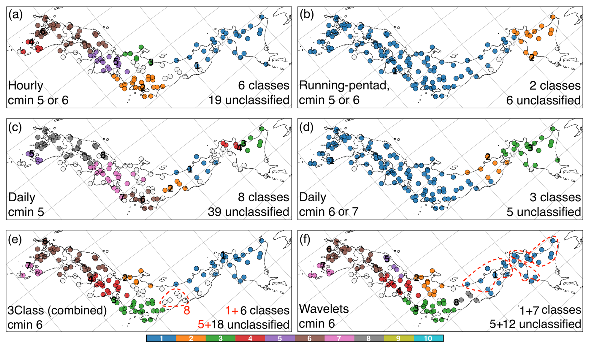
Figure 3 Rain-gauge clusters. Labels of clusters based on the time series of June–July (a) 99th percentile hourly rainfall using c_min=5 or c_min=6; (b) 90th percentile running-pentad rainfall using c_min=5 or c_min=6; (c) 90th percentile daily rainfall using c_min=5; (d) 90th percentile daily rainfall using c_min=6. (e) Labels of station groups with the same combination of hourly, daily, and running-pentad clusters using c_min=6 (3Class). The dashed red contour shows the manual addition of cluster 8; red text lists the number of unclassified stations that fall in the manually added cluster 8. Cluster label 5 is missing in this panel. (f) Labels of clusters using the wavelet-based metric with c_min=6, including the manual addition of one c_min=5 cluster as cluster 8. Dashed red contours show three c_min=5 clusters that merged to form cluster 1 when c_min=6. The numbers of classes (referring to either clusters or 3Class) and unclassified rain gauges are shown on the bottom right. Colours only reflect the cluster numbering and do not reflect any units or magnitudes. White markers show unclassified rain gauges. Longitude–latitude grid lines are shown as grey lines; the map is a rotated projection.

There were three clusters for Hokkaido island, represented by clusters 3 and 4 and the unclassified rain gauges on the southern coast in Fig. 3c. These may merge into one larger cluster (cluster 2 in Fig. 3b; cluster 3 in Fig. 3d). There were two clusters over the Tohoku region, represented by clusters 1 and 2 in Fig. 3c. The northern cluster (cluster 1) may either merge northwards (Fig. 3a) or southwards (Fig. 3b) into larger clusters. The southern cluster (cluster 2) usually merged southwards (cluster 1 in Fig. 3b and d). There was a large cluster in the Kanto region, represented by cluster 2 in Fig. 3a and cluster 6 in Fig. 3c. The size and boundary of this cluster varied, especially at its western coastal side and northern mountainous side; north of it was a small cluster on the Sea of Japan coast (cluster 3 in Fig. 3a), while west of it was a cluster in the Kansai region (cluster 5 in Fig. 3a and cluster 7 in Fig. 3c). There was a large cluster covering most of the Chugoku region and Kyushu island, represented by cluster 6 in Fig. 3a and cluster 8 in Fig. 3c. Finally, there was a small cluster at the southern tip of Kyushu that was quite robust, persisting through multiple values of c_min, represented by cluster 4 in Fig. 3a and cluster 5 in Fig. 3c. The five clusters from Kanto to Kyushu may merge into one larger cluster (cluster 1 in Fig. 3b and d). Most rain gauges along the Pacific coast of Shikoku island and Kinki were initially unclassified and only merged into this larger cluster as c_min increased to larger values.

The optimal value c_min=6 was common between the three temporal resolutions. Figure 3e shows 3Class rain-gauge groups with the same combination of cluster labels from using c_min=6 on the three temporal resolutions, excluding 23 rain gauges containing any unclassified label. Six 3Class groups emerged, with the “5” label skipped for later comparison with Fig. 3f. The northernmost was a four-in-one large cluster consisting of the combination of the three Hokkaido clusters and the northern Tohoku cluster. The southern Tohoku cluster was at first excluded because it consisted of five rain gauges, which became unclassified for hourly extremes when c_min=6 (Fig. 3a). It was manually added to create a total of seven 3Class groups (dashed red contour labelled “8” in Fig. 3e).

Figure 4 shows the clusters returned with different c_min values using the wavelet metric. Starting from c_min=3 produced 19 clusters and 23 unclassified rain gauges (boxes a–s in Fig. 4). Increasing to c_min=4 produced 12 clusters with 22 unclassified rain gauges; five smaller clusters for Kyushu island and Chugoku region merged (boxes n–r in Fig. 4; cluster 6 in Fig. 3f), but the cluster at the southern tip of Kyushu (box m in Fig. 4; cluster 7 in Fig. 3f) and the cluster on the Sea of Japan coast (box s in Fig. 4; cluster 5 in Fig. 3f) would persist until c_min=11. Increasing to c_min=5 produced nine clusters with 20 unclassified rain gauges; three smaller clusters in the Kanto region merged into one (boxes i–k in Fig. 4; cluster 3 in Fig. 3f). A notable change took place at c_min=6, which produced seven clusters and 18 unclassified rain gauges. Hokkaido and northern Tohoku clusters merge into one cluster (boxes a–e in Fig. 4; cluster 1 in Fig. 3f). However, the southern Tohoku cluster of five rain gauges became unclassified (box f in Fig. 4). The clusters remained largely unchanged until c_min=11, except that the Sea of Japan cluster of six rain gauges also became unclassified at c_min=7. Hence, c_min=6 was optimal for producing a small number of large clusters, as shown in Fig. 3f. The southern Tohoku cluster was manually added to create a total of eight analysis regions and 12 unclassified rain gauges (box f in Fig. 4; cluster 8 in Fig. 3f). The specific rain gauges that make up these regions have been listed in Table 1.

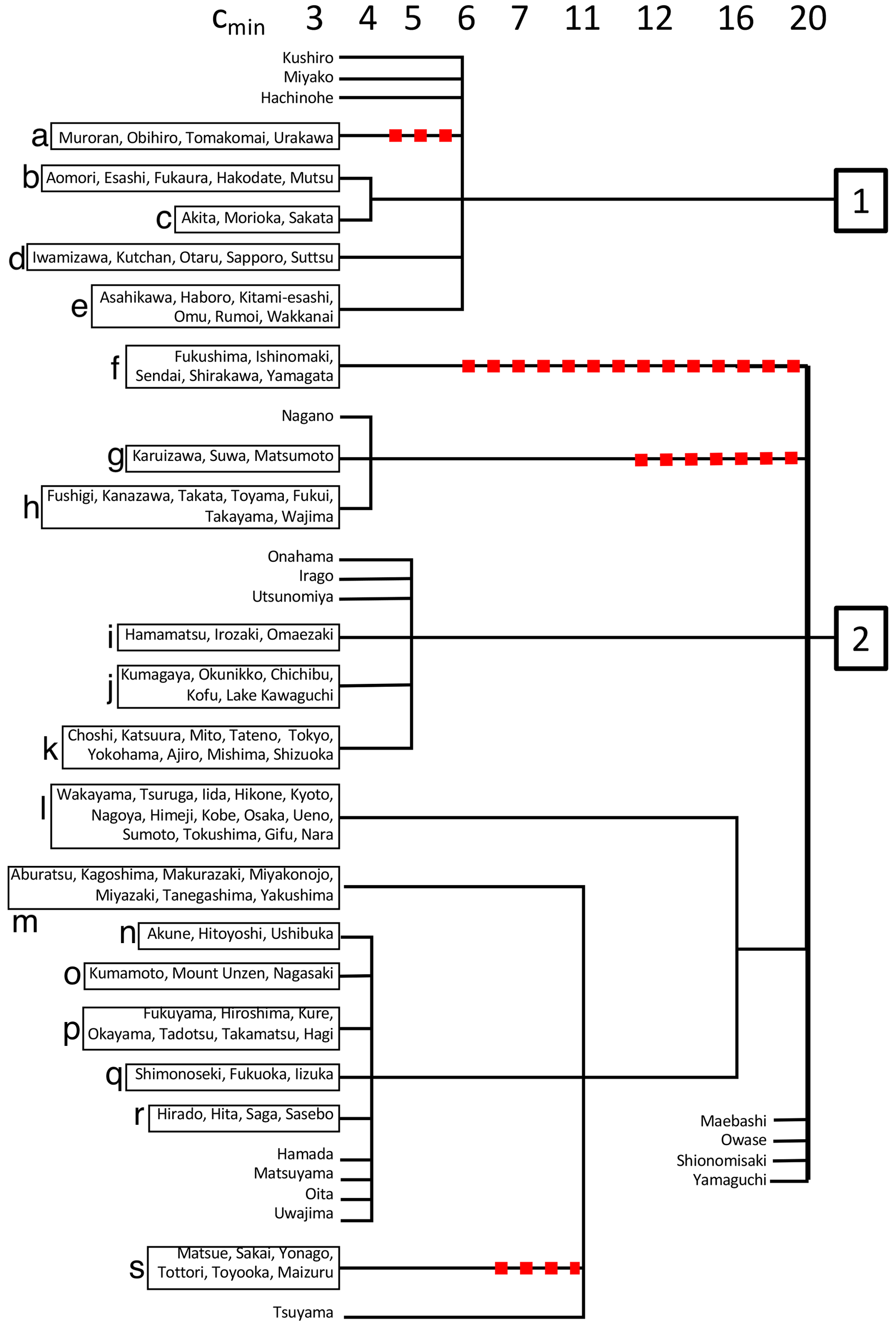
Figure 4 Dendrogram using the wavelet-based metric, showing the combination of rain gauges into clusters with different values of c_min, starting from 19 clusters when c_min=3. Red dashes indicate that the rain gauges in the boxes became unclassified because the cluster size was smaller than c_min. These unclassified rain gauges later merged back into larger clusters.

The result of individually clustering three temporal resolutions to create 3Class groups from unique combinations of cluster labels and the result of the wavelet-based clustering were compared in Fig. 3e and f. The same optimal c_min=6 was found in both methods. The value of c_min can be reduced to produce better geographical resolution, since most of the smaller clusters appeared robust between methods. On the other hand, increasing c_min further would not produce interesting clusters from the perspective of a regional study since the results would resemble Fig. 3b or 3d. The clusters produced by the two methods were highly similar. The most notable difference was that 3Class cluster 6 in Fig. 3e split into two wavelet-based clusters (clusters 5 and 6 in Fig. 3f). Minor differences were that clusters 1 and 2 were larger from the wavelet-based method than the 3Class method. The wavelet-based method is better than the 3Class method in that it included multiple temporal frequencies in one round of clustering and produced a single clustering tree that was more easily interpretable.

The wavelet-based clustering method was next applied to d4PDF. When c_min=8, most points suddenly merged into one large cluster covering the entire study domain. Therefore, c_min=7 was used, and the result is shown in Fig. 5a. There were 1501 small clusters, a number which appeared excessively large. To make sense of this, three wavelet components were independently clustered. These were D1 corresponding to periods of 2–4 h, D4 corresponding to periods of 1.3–2.7 d, and D6 corresponding to periods of 5.3–10.7 d. Figure 5b shows the results of clustering D1 with the largest usable c_min=7, producing 898 classes. Clusters with similar (purple) labels were found for Kyushu and along the Pacific coast of western Japan. Figure 5c shows the results of clustering D4 with the largest usable c_min=8, producing 1165 clusters. The linear pattern along the Pacific coast had broken apart. In particular, cluster labels over Kyushu were split into western (purple) and eastern (orange–yellow) groups. Figure 5d shows the results of clustering D6 with the largest usable c_min=25, producing 282 clusters. Clusters with similar (orange–yellow) labels now covered the whole of Kyushu, inland, and the Sea of Japan coast of northeast Japan. Purple labels were found over the region corresponding to cluster 5 in Fig. 3f and the Pacific coast from Kanto to Hokkaido. The change between two coast-aligned patterns from high to low temporal frequencies likely contributed to the fragmentation into many clusters. Illustrating this with rain gauges, c_min=5 produced six hourly, eight daily, and two running-pentad clusters, but these combined into nine 3Class groups (10 with the manual addition of the southern Tohoku cluster).

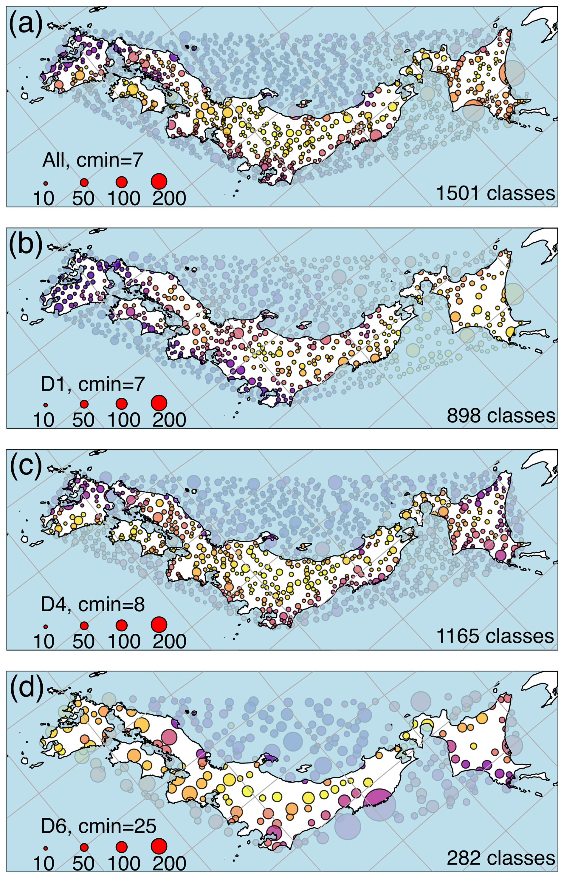
Figure 5 d4PDF labels and sizes of clusters using the time series of June–July rainfall after wavelet decomposition. (a) All components. (b) D1 component only, containing signals of periods 4–8 h. (c) D4 component only, containing signals of periods 1.3–2.7 d. (d) D6 component only, containing signals of periods 5.3–10.7 d. Colours only reflect the cluster numbering and do not reflect any units or magnitudes. Circle marker sizes reflect cluster sizes (legend). A translucent blue mask was used to cover data within the convex hull used for clustering but falling inside the ocean. Longitude–latitude grid lines are shown as grey lines; the map is a rotated projection.

Another contributing factor was likely the limitation by the finest denominator of clustering. The D6 component could be clustered with c_min=25 into 282 clusters of relatively large size, so the overall c_min=7 threshold was likely due to the D1 component, which had the same c_min=7 threshold. To test if larger clusters could be formed by considering more distant points as cluster candidates, D1 was reclustered after doubling the calculation radius S_calc from 1–2°, then from 2–4°. The results were unchanged, indicating that the cause was the lack of significantly correlated points inside the domain at this frequency range, rather than artificial limitation by S_calc. Even if clustering were limited to D6, the 282 D6 clusters were still very large compared to even the c_min=3 rain-gauge result of 19 clusters. The reason for the large number of clusters is not clear. It is possible that clustering methodology must be further adapted for use on the high-resolution ensemble simulations.

3.3 Correlation coefficients (R)

Before correlating rainfall extremes with the Pacific SST modes, the values from rain gauges and co-located d4PDF clusters were compared. Figure 6 shows the distributions of rainfall extremes for the eight analysis regions. The whisker ranges of values from rain gauges and d4PDF overlapped in all comparison cases, although the distribution peaks of d4PDF were always of smaller value than that of the rain gauge. The latter was not surprising since the model was of 5 km horizontal resolution, and we expect rainfall extremes to improve with model resolution in the future. Hourly and daily extremes were better simulated than running-pentad extremes. The quartile bars of rain gauges and d4PDF overlapped except for region 5 (western Sea of Japan coast; Fig. 6c). For running-pentad extremes, the quartile bars of rain gauges and d4PDF overlapped only for region 3 (Kanto; Fig. 6f). The difference in performance between daily and running-pentad resolutions suggests that rain gauges experienced more continuous rainfall in 5 d periods but the model less so. Distributions of hourly extremes from d4PDF were bimodal or trimodal in most cases but from rain gauges only obviously so for region 2 (central Sea of Japan coast; Fig. 6e); d4PDF performed the best over region 3 (Kanto; Fig. 6f) and worst over region 5 (western Sea of Japan coast; Fig. 6c). The good performance over region 3 may be due to it being topographically flat. In contrast, region 5 was a topographically complex region with steep topography near a coastline.

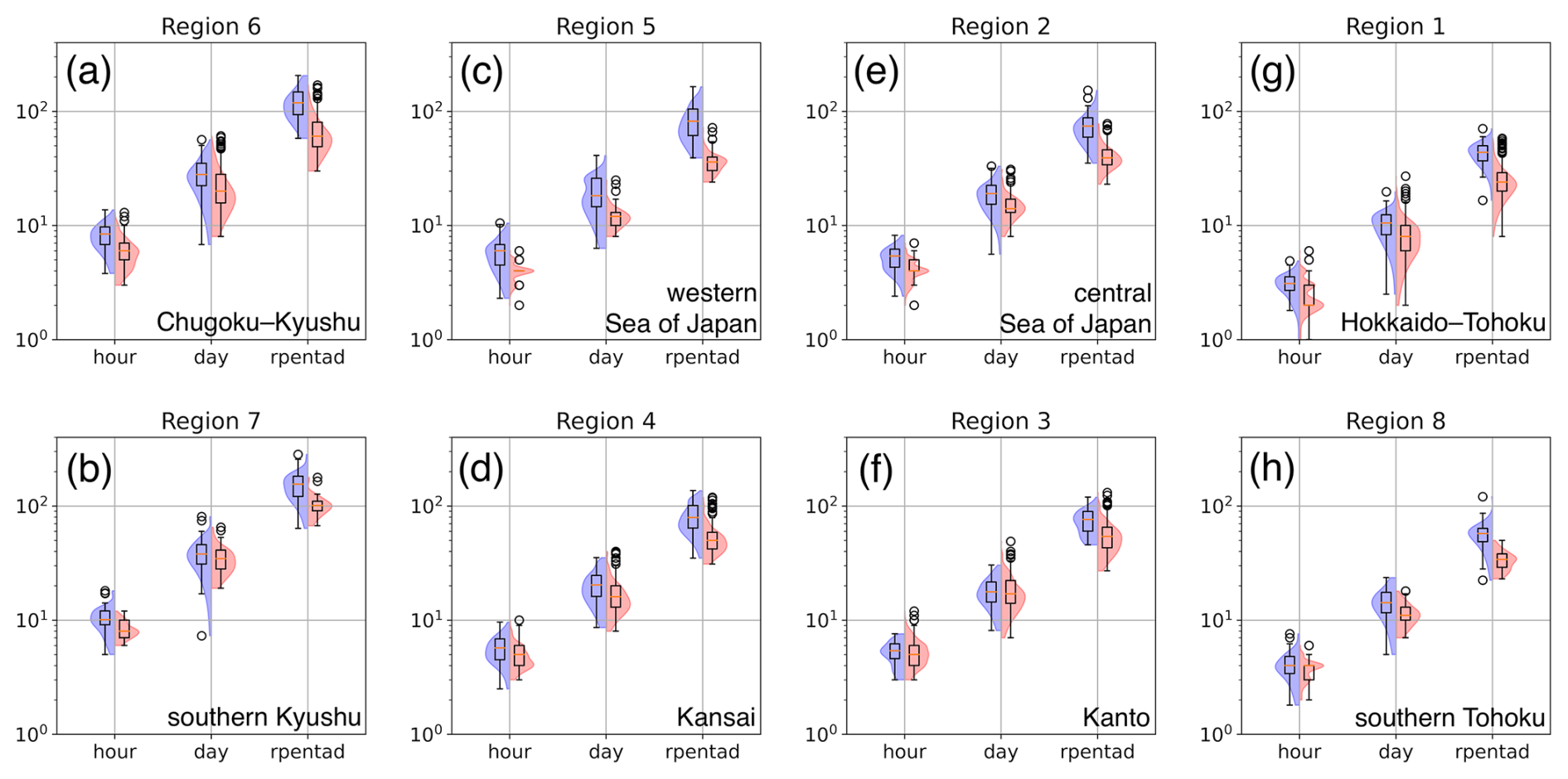
Figure 6 The distribution of June–July 99th percentile hourly rainfall (“hour”), 90th percentile daily rainfall (“day”), and 90th percentile running-pentad rainfall (“rpentad”) in millimetres. The eight analysis regions are arranged by their geographical location from southwest to northeast in Fig. 3f. Left side (blue shading) shows the distribution from rain gauges, where each sample is the annual percentile value of the cluster. Right side (red shading) shows the distribution from d4PDF, where each sample is the annual percentile of each cluster co-located with the rain gauges. Bar-and-whisker plots show the 1st and 3rd quartile values as boxes, whiskers extended out 1.5 times the 1st-to-3rd interquartile range, and circle markers showing outliers.

Figures 7–9 show the R values between rainfall extremes and standardised scores of the Pacific SST modes, at three temporal resolutions. Figure 10 summarises the results by analysis region. The left columns of Figs. 7–9 show R values for individual rain gauges, which were at most weak. By individual rain gauges, field significance was found for correlation with Trend+ for hourly extremes (12 significant rain gauges) and anti-correlation with PDV for daily extremes (13 significant rain gauges). Rain gauges correlated with Trend+ for hourly extremes were scattered over the study domain, but more were found on the east side of Kyushu island and in eastern Japan near the Kanto region (Fig. 7c). Due to their scattered nature, only analysis region 7 showed a significant hourly relationship of R=0.31 (southern Kyushu; first bar of mode 3 in Fig. 10b). Region 3 showed hourly R=0.22 close to but not exceeding the significance threshold (Kanto; first bar of mode 3 in Fig. 10f). Rain gauges anti-correlated with PDV for daily extremes were mostly found on Shikoku island and Hokkaido island (Fig. 8d). Most rain gauges on Shikoku, specifically Pacific-facing locations, were unclassified by clustering. Region 1 showed significant daily relationship of $R=-\mathrm{0.28}$ (Hokkaido–Tohoku; second bar of mode 4 in Fig. 10g).

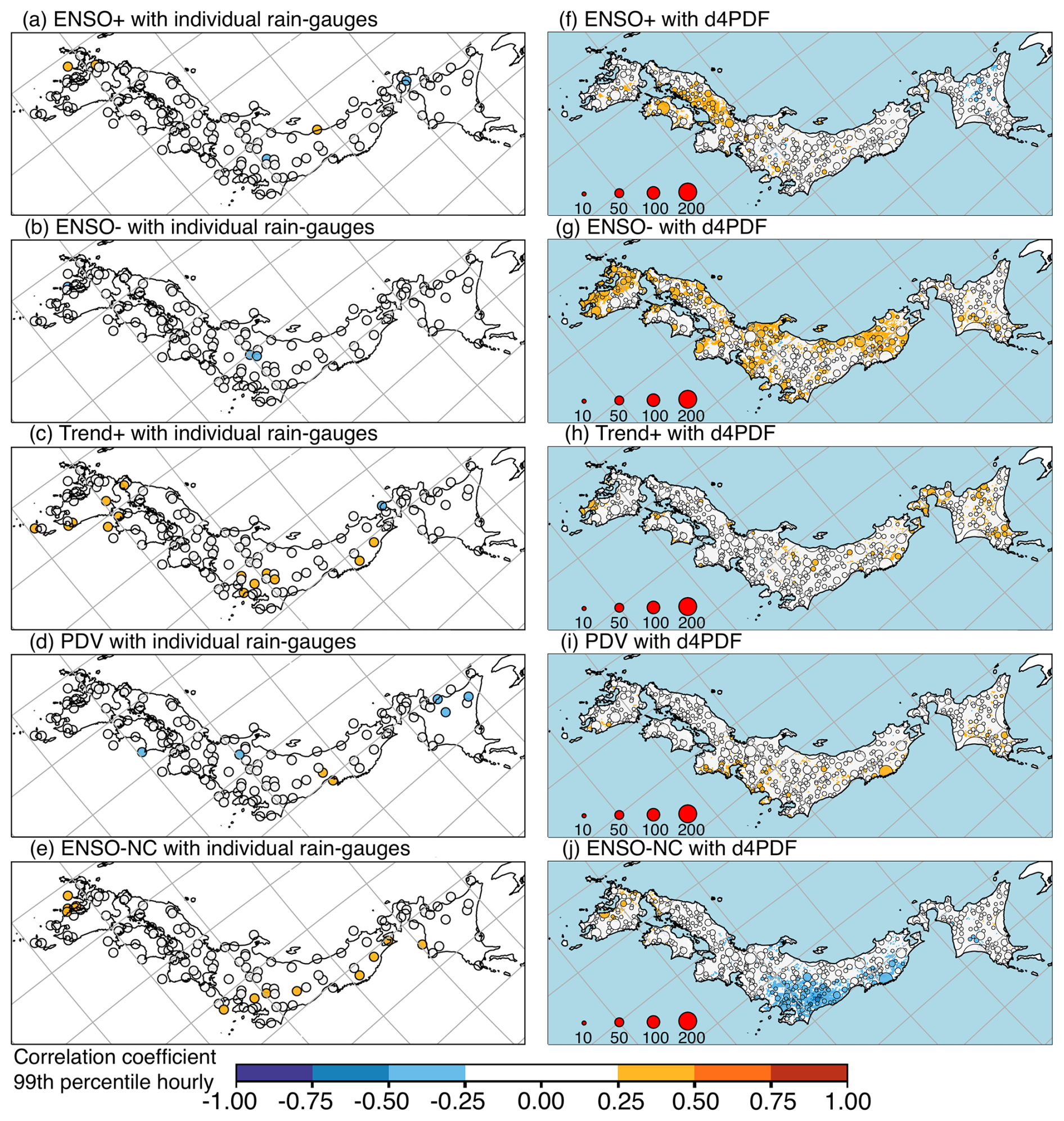
Figure 7 Spearman correlation coefficients (R) for the 1952–2010 period between the scores of five Pacific SST modes (rows) and 99th percentile hourly rainfall from rain gauges (a–e) or d4PDF (f–j). June–July rainfall extremes of individual rain gauges with (a) ENSO+, (b) ENSO-, (c) Trend+, (d) PDV, and (e) ENSO-NC. June–July rainfall extremes of d4PDF sets with (f) ENSO+, (g) ENSO-, (h) Trend+, (i) PDV, and (j) ENSO-NC. In the right column, circle marker sizes reflect cluster sizes, while single points are shown as coloured dots. A blue mask was used to cover d4PDF data inside the ocean. Longitude–latitude grid lines are shown as grey lines; the map is a rotated projection.

Figure 8 Same as Fig. 7 but for June–July 90th percentile daily rainfall.

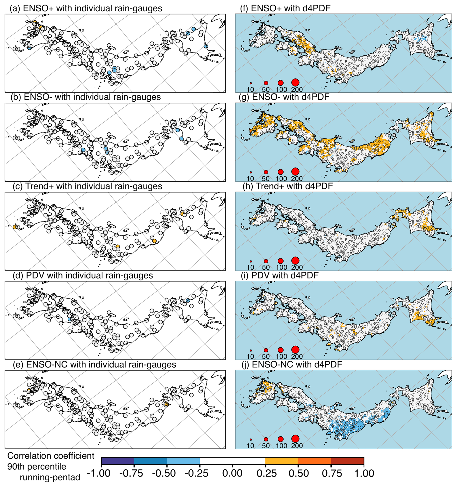
Figure 9 Same as Fig. 7 but for June–July 90th percentile running-pentad rainfall.

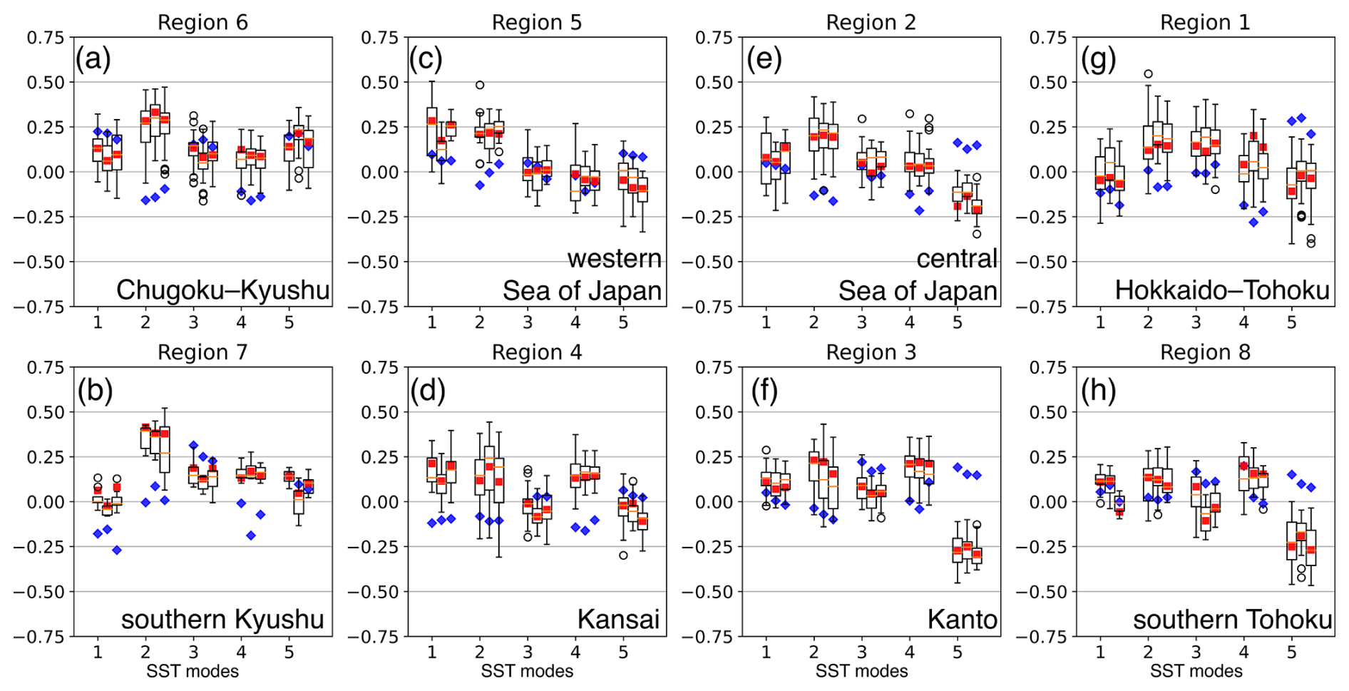
Figure 10 Spearman correlation coefficients (R) between June–July rainfall extremes and the scores of the first five Pacific SST modes. The eight analysis regions are arranged by their geographical location from southwest to northeast in Fig. 3f. Three columns for each mode show the results for 99th percentile hourly, 90th percentile daily, and 90th percentile running-pentad rainfall. Blue diamonds represent the R values from rain-gauge cluster. Bar-and-whisker plots show the first and third quartile values as boxes, whiskers extended out 1.5 times the first-to-third interquartile range, and circle markers showing outliers. Red boxes show the mean of d4PDF R values weighted by cluster size.

Besides these larger patterns, there were rain gauges concentrated over northwestern Kyushu correlated with ENSO+ for daily extremes (Fig. 8a), over Kanto anti-correlated with ENSO+ for running-pentad extremes (Fig. 9a), over Hokkaido anti-correlated with PDV for hourly extremes (Fig. 7b), over west Kyushu correlated with ENSO-NC for hourly and daily extremes (Figs. 7e and 8e), and along the Pacific coast of eastern Japan with ENSO-NC for hourly extremes (Fig. 7e). However, these relationships were not seen for the analysis regions that contained these subsets of rain gauges except for the last, reflected in region 1, which showed a significant hourly relationship of R=0.28 (Hokkaido–Tohoku; first bar of mode 5 in Fig. 10g).

Besides the regional relationships described above, region 7 showed a significant running-pentad relationship with ENSO+ of $R=-\mathrm{0.27}$ (southern Kyushu; third bar of mode 1 in Fig. 10b), and region 1 showed significant daily relationships with ENSO-NC of R=0.30 (Hokkaido–Tohoku; second bar of mode 5 in Fig. 10g). Examination of Fig. 9a shows that the first relationship derives from only one rain gauge in the cluster. Examination of Fig. 8e suggests that the second relationship is believable since it was derived for four rain gauges and was consistent with the hourly ENSO-NC relationship. Considering regions (clusters) as samples, there was no cluster-wise field significance with any SST mode, which required significance for at least three of eight regions.

The right columns of Figs. 7–9 show R values for d4PDF clusters, which were at most weak, except for the relationship between hourly extremes and ENSO-NC, where a few moderately anti-correlated clusters were seen for eastern Japan (Fig. 7j). The spatial correlation patterns in d4PDF were different from those in the rain gauges. Correlation with ENSO+ was seen over Chugoku for hourly and running-pentad extremes (Figs. 7f and 9f). This was significant for clusters co-located with rain gauges of region 5 (western Sea of Japan coast; Fig. 10c). The relationship was not seen in the rain gauges, although this may be a spatial bias where observed positive correlation over northwest/west Kyushu was shifted northeastwards in d4PDF. Correlation with ENSO- was seen over western Kyushu and some places along the Sea of Japan coast (Figs. 7g, 8g, and 9g). This was significant for clusters co-located with rain gauges of regions 6 and 7 (Fig. 10a and b). The relationship was excessively strong and not seen in the rain gauges, so it can be considered a strength bias. Correlation with Trend+ was seen over some parts of Hokkaido (Figs. 7h, 8h, and 9h). This may be a spatial bias from the rain gauges, where correlation was seen in regions south of Hokkaido but not for Hokkaido. Correlation with PDV was seen over eastern Kyushu and southeast Hokkaido for daily and running-pentad extremes (Figs. 8i and 9i). This was strength bias from the rain gauges, which only showed anti-correlation. Correlation with ENSO-NC was seen over some parts of western Kyushu, while anti-correlation with ENSO-NC was seen over eastern Japan (Figs. 7j, 8j, and 9j). This was significant for clusters co-located with rain gauges of region 3 (Kanto) in Fig. 10f. The anti-correlation over eastern Japan was excessive and not seen in rain gauges, resulting in a strength bias.

The relative performance of d4PDF for the different SST modes can be evaluated from Fig. 10. We required that the rain-gauge R values (blue diamonds) fall within the range of d4PDF R values (boxplot whiskers), for at least two out of three temporal resolutions, to call the model performance acceptable. For ENSO+, this was six of eight regions (6, 5, 2, 1; 3, and 8, listed along rows with top and bottom rows divided by a semicolon). For ENSO-, this was three regions (4, 3, 8). For Trend+, this was seven regions (6, 5, 2, 1; 7, 4, 8). For PDV, this was three regions (5; 3, 8). For ENSO-NC, this was four regions (6, 5; 7, 4). The best performance by region was for ENSO+ and Trend+, although in almost all cases acceptable performance meant reproducing the lack of relationship. The Trend+ mode was described in Sect. 3.1 as including both warming trend and interannual and decadal variability, so we would like to further investigate its relationship with rainfall extremes.

To better evaluate the relationships between rainfall extremes and warming alone, Trend+ scores were smoothed using an 11-year running mean (dotted black line in Fig. 1c). Figure 11 shows the correlations with this smoothed trend. Figure 12 summarises the results by analysis region, also including regional relationships with the NPGO index, TPI, and SOI. The spatial patterns for the other three indices are not shown, because the relationships were unremarkable and no better than those for the SST modes. In these figures, the threshold for significance was $\left|R\right|>\mathrm{0.27}$ due to the shorter time period after smoothing. Due to this higher threshold, there was no domain-wide field significance by considering individual rain gauges. Although Fig. 11a showed a number of weakly correlated rain gauges similar to Fig. 7a, including one moderately correlated rain gauge at southern Kyushu, only 10 rain gauges were significantly correlated. Nevertheless, the spatial distribution of correlated rain gauges for Kyushu and anti-correlation rain gauges for the inland region further northeast seemed (by eye) similar between the three temporal resolutions (Fig. 11a–c); d4PDF seemed to show a similar spatial pattern, except for the presence of correlated regions for Hokkaido that were not seen in rain gauges (Fig. 11d–f).

Figure 11 Spearman correlation coefficients (R) for the 1957–2006 period between 11-year running mean of the Trend+ score June–July and rainfall extremes of different temporal resolution (rows), from individual rain gauges (a–c) or d4PDF (d–f). From rain gauges, (a) 99th percentile hourly rainfall, (b) 90th percentile daily rainfall, (c) 99th percentile running-pentad rainfall. From d4PDF, (d) 99th percentile hourly rainfall, (e) 90th percentile daily rainfall, (f) 99th percentile running-pentad rainfall. In the right column, circle marker sizes reflect cluster sizes, while single points are shown as coloured dots. A blue mask was used to cover d4PDF data in the ocean. Longitude–latitude grid lines are shown as grey lines; the map is a rotated projection.

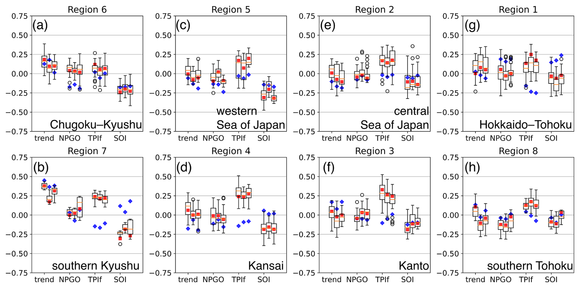
Figure 12 Same as Fig. 10 but with the 11-year running mean Trend+ score, NPGO index, the TPI (filtered version), and the SOI.

By analysis region, only region 7 (southern Kyushu) showed significant correlation. This was for all three temporal resolutions with hourly R=0.45, daily R=0.36, and running-pentad R=0.38 (trend mode in Fig. 12b). The model performance with smoothed trend was acceptable for the same seven regions as Trend+ (6, 5, 2, 1; 4, 3, 8). In region 7, model R values were also high, but their range fell short of the rain-gauge values for hourly and daily extremes (first and second bars of trend mode in Fig. 12b). Model performance with the NPGO index was acceptable for six regions (2, 1; 7, 4, 3, 8). For TPI, this was only three regions (6, 5, 2). For SOI, this was five regions (6, 5, 2; 3, 8), the same regions as ENSO+ excluding region 1 (Hokkaido–Tohoku). It seems that d4PDF produced appropriate relationships between hourly rainfall extremes and the slow components of Trend+, except for over Hokkaido; d4PDF should be used with caution when studying ENSO and PDV due to the above-described biases.

4 Discussion

The lack of strong R values between rainfall extremes and scores of the Pacific SST modes indicates that the SST modes were not major controlling factors for extreme rainfall over Japan. These results are sensible in that extreme rainfall typically occurs in mesoscale systems that may be associated with certain synoptic-scale conditions but are much less likely to be directly caused by hemisphere- or planetary-scale climate variability. In this section, rainfall extremes were correlated against indices reflecting the state of the regional monsoon near Japan to check if there were stronger relationships with regional conditions. Rain-gauge rainfall extremes were correlated with monsoon indices calculated from JRA55, and these relationships were considered observations, shown on the left columns of Figs. 13–18; d4PDF rainfall extremes were correlated with monsoon indices calculated from d4PDF-AGCM, shown on the right columns of Figs. 13–18. Figure 19 summarises the results by analysis region.

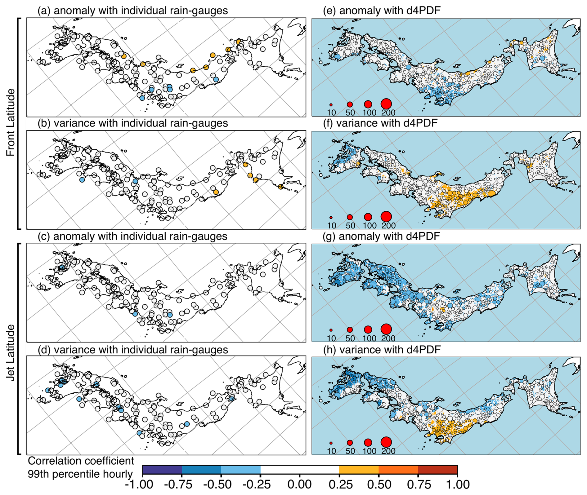
Figure 13 Spearman correlation coefficients (R) for the 1958–2010 period between monsoon indices related to position (rows) and June–July 99th percentile hourly rainfall from rain gauges (a–d) or d4PDF (e–h). Left column shows R values for rainfall extremes of individual rain gauges with JRA55 monsoon indices: (a) seasonal anomaly of monsoon front latitude μ_FLat, (b) seasonal variance of monsoon front latitude ${\mathit{\sigma }}_{\text{FLat}}^{\mathrm{2}}$, (c) seasonal anomaly of monsoon jet latitude μ_JLat, and (d) seasonal variance of monsoon jet latitude ${\mathit{\sigma }}_{\text{JLat}}^{\mathrm{2}}$. Right column shows R values for rainfall extremes of d4PDF sets with d4PDF monsoon indices: (e) μ_FLat, (f) ${\mathit{\sigma }}_{\text{FLat}}^{\mathrm{2}}$, (g) μ_JLat, and (h) ${\mathit{\sigma }}_{\text{JLat}}^{\mathrm{2}}$. In the right column, circle marker sizes reflect cluster sizes, while single points are shown as coloured dots. A blue mask was used to cover d4PDF data in the ocean. Longitude–latitude grid lines are shown as grey lines; the map is a rotated projection.

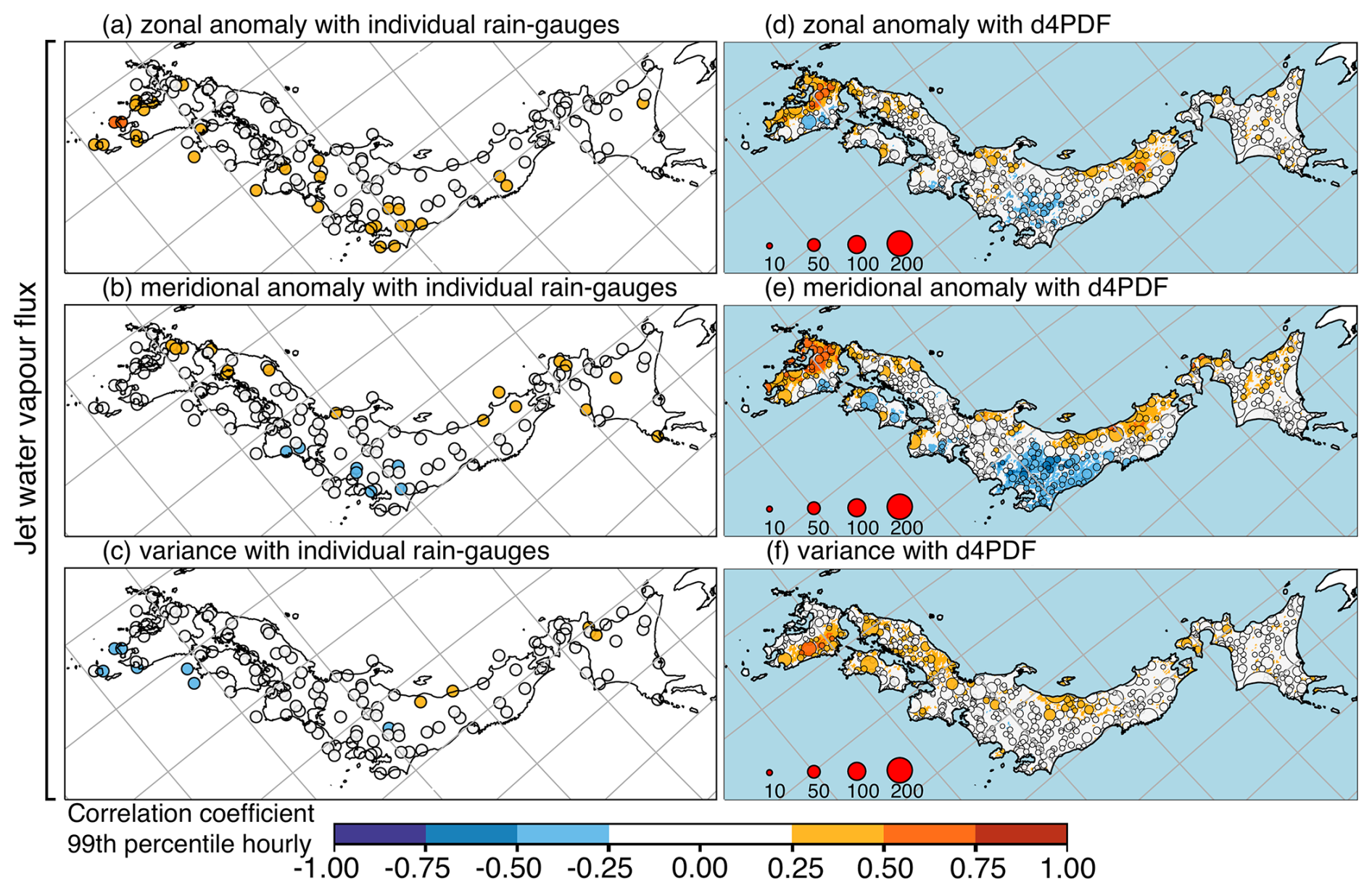
Figure 14 Same as Fig. 13 but using monsoon indices related to the strength of the monsoon jet. Left column (a–c) shows R values for rainfall extremes of individual rain gauges with JRA55 monsoon indices: (a) seasonal anomaly of the monsoon jet zonal water vapour flux μ_QU, (b) seasonal anomaly of the monsoon jet meridional water vapour flux μ_QV, and (c) seasonal variance of the monsoon jet water vapour flux ${\mathit{\sigma }}_{Q(U,V)}^{\mathrm{2}}$. Right column (d–f) shows R values for rainfall extremes of d4PDF sets with d4PDF indices: (d) μ_QU, (e) μ_QV, and (f) ${\mathit{\sigma }}_{Q(U,V)}^{\mathrm{2}}$.

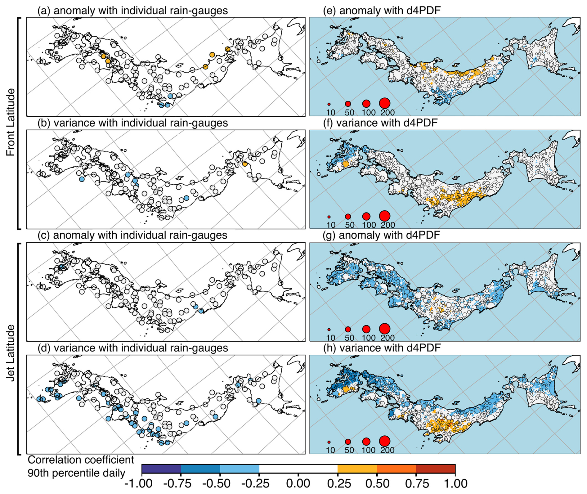
Figure 15 Same as Fig. 13 but for 90th percentile daily rainfall.

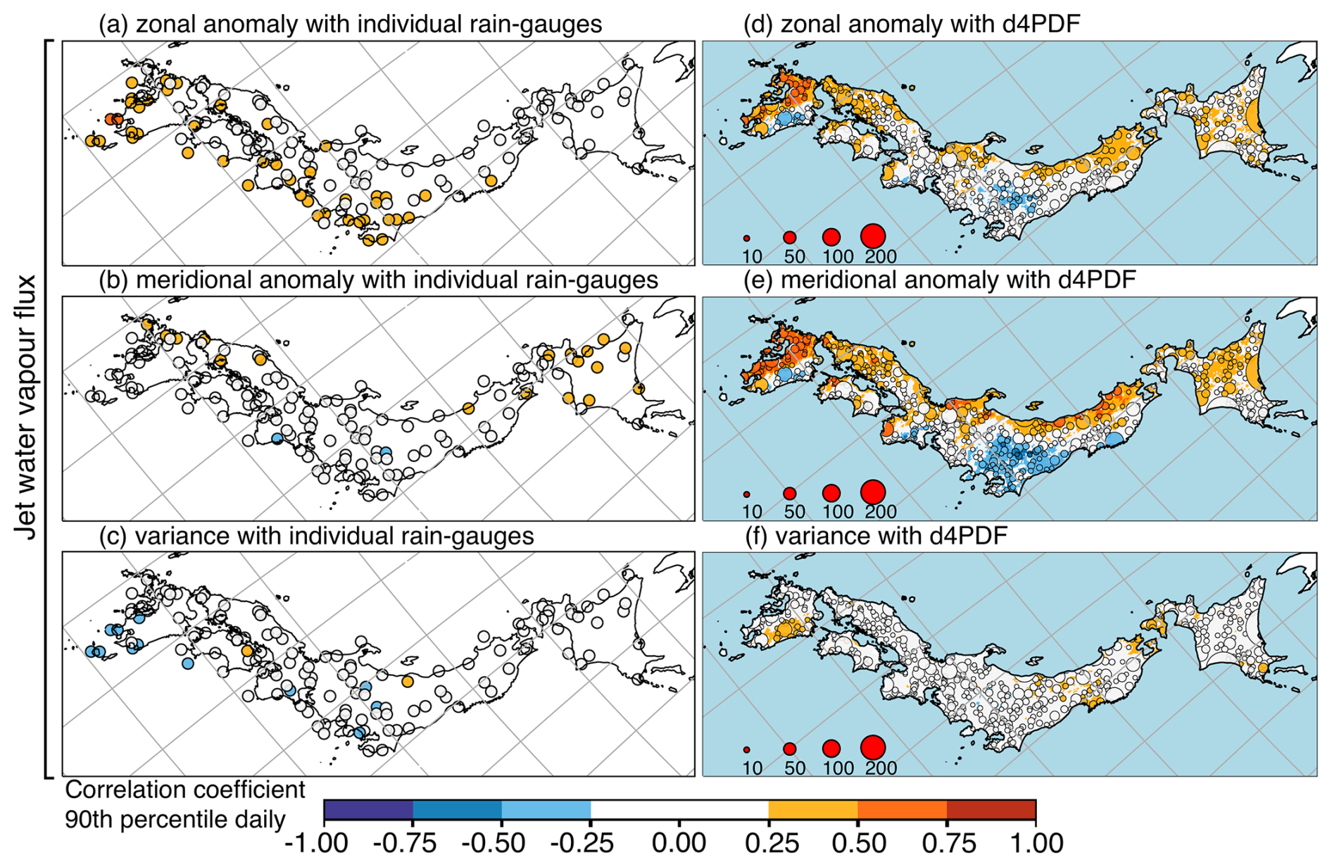
Figure 16 Same as Fig. 14 but for 90th percentile daily rainfall.

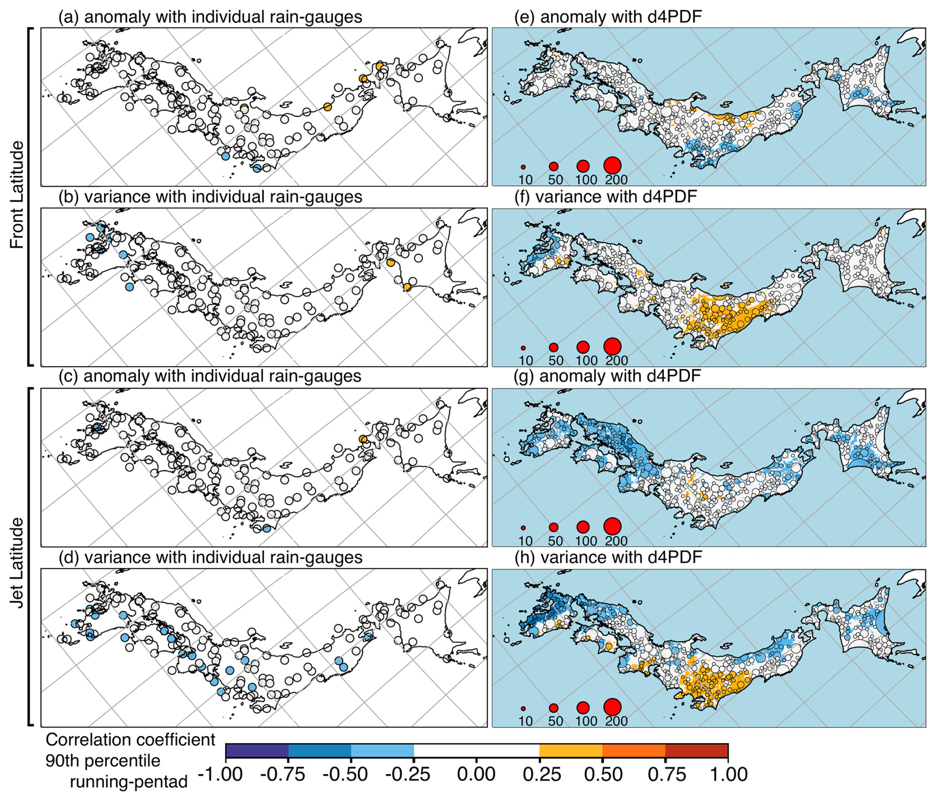
Figure 17 Same as Fig. 13 but for 90th percentile running-pentad rainfall.

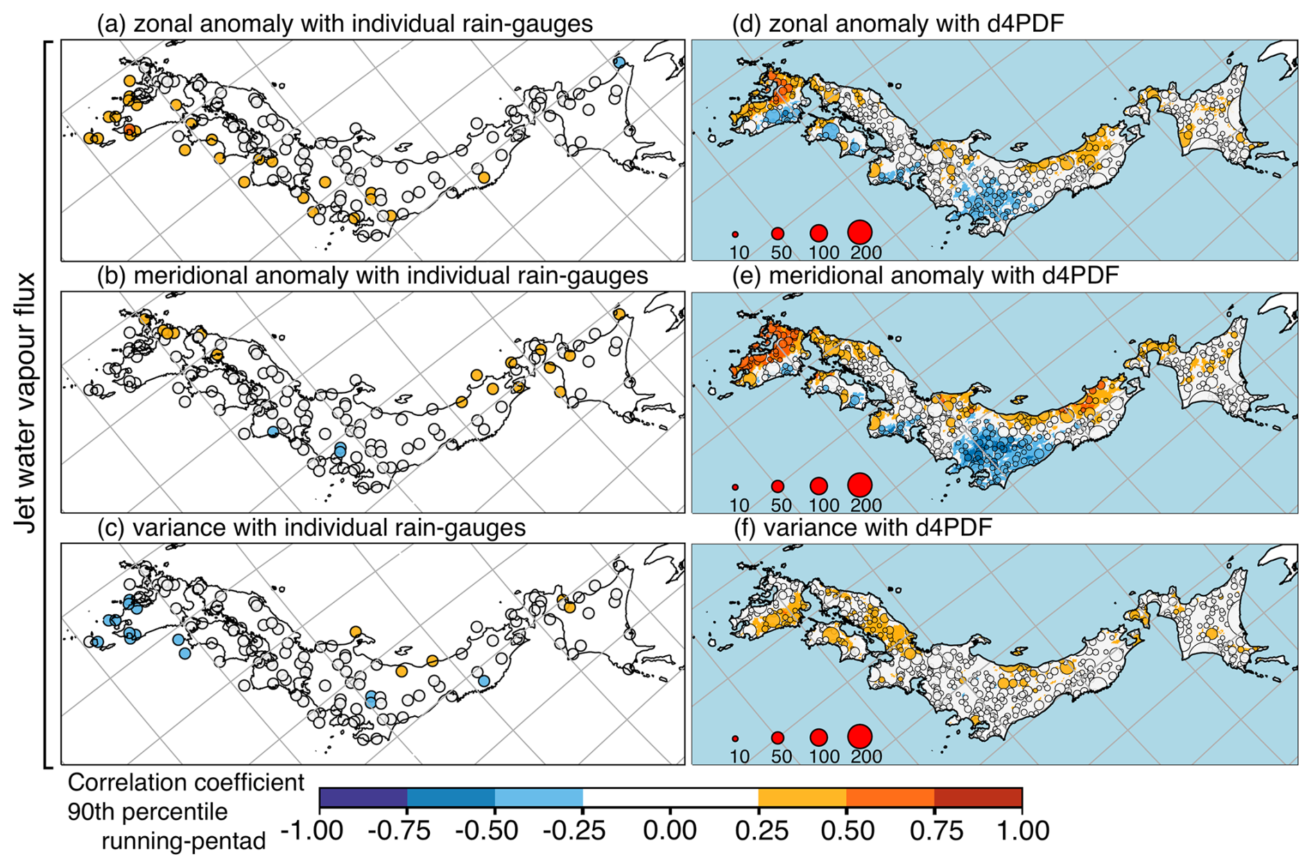
Figure 18 Same as Fig. 14 but for 90th percentile running-pentad rainfall.

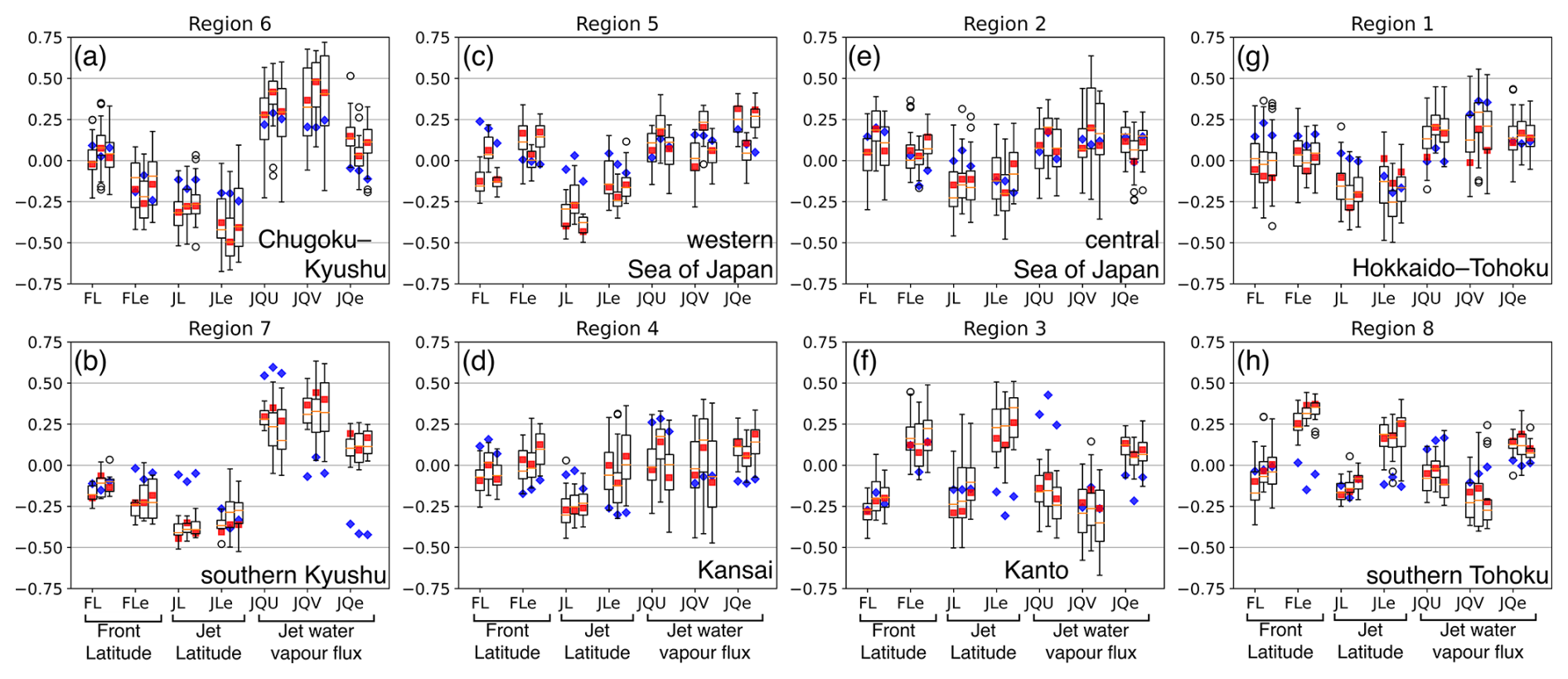
Figure 19 Same as Fig. 10 but using regional monsoon indices. FL and FLe represent monsoon front latitude indices μ_FLat and ${\mathit{\sigma }}_{\text{FLat}}^{\mathrm{2}}$. JL and JLe represent monsoon jet latitude indices μ_JLat and ${\mathit{\sigma }}_{\text{JLat}}^{\mathrm{2}}$. JQU, JQV, and JQe represent monsoon jet water vapour flux indices μ_QU, μ_QV, and ${\mathit{\sigma }}_{Q(U,V)}^{\mathrm{2}}$.

Based on observations, rainfall extremes showed up to moderate correlation only with the seasonal (June–July) anomaly of monsoon jet zonal strength (μ_QU; Figs. 14a, 16a, and 18a). Considering individual rain gauges, domain-wide field significance was found for correlation with μ_QU using all three temporal resolutions of hourly extremes (25 rain gauges; Fig. 14a), daily extremes (36 rain gauges; Fig. 16a), and running-pentad extremes (24 rain gauges; Fig. 18a). The correlated rain gauges were concentrated along the Pacific coast of western Japan. The relationship was reflected in significant cluster correlations in region 7 with hourly R=0.55, daily R=0.60, and running-pentad R=0.56 (southern Kyushu; JQU in Fig. 19b); in region 3 with hourly R=0.31 and daily R=0.43 (Kanto; first and second bars of JQU in Fig. 19f); in region 4 with daily R=0.28 (Kansai; second bar of JQU in Fig. 19d); and in region 6 with daily R=0.29 (Chugoku–Kyushu; second bar of JQU in Fig. 19a). This meant that cluster-wise field significance was found for daily correlation with μ_QU.

The rest of the indices showed at most weak relationships, similar to the relationships with SST modes. However, rainfall extremes had better relationships with some monsoon indices in the sense that more rain gauges showed significant relationships. Field significance was also found for correlation with the seasonal meridional anomaly of monsoon jet meridional strength (μ_QV) using all three temporal resolutions of hourly extremes (12 rain gauges; Fig. 14b), daily extremes (15 rain gauges; Fig. 16b), and running-pentad extremes (14 rain gauges; Fig. 18b). The μ_QV-correlated rain gauges were concentrated along the Sea of Japan coast. Only region 1 showed significant correlation at all three temporal resolutions with hourly R=0.28, daily R=0.36, and running-pentad R=0.35 (Hokkaido–Tohoku; JQV in Fig. 19g).

Both the seasonal variance of monsoon jet latitude (${\mathit{\sigma }}_{\text{JLat}}^{\mathrm{2}}$) and the seasonal variance of monsoon jet strength (${\mathit{\sigma }}_{Q(U,V)}^{\mathrm{2}}$) were indicators of monsoon jet instability, but ${\mathit{\sigma }}_{\text{JLat}}^{\mathrm{2}}$ was better related to rainfall extremes than ${\mathit{\sigma }}_{Q(U,V)}^{\mathrm{2}}$. Field significance was found for anti-correlation with ${\mathit{\sigma }}_{\text{JLat}}^{\mathrm{2}}$ using daily extremes (28 rain gauges; Fig. 15d) and running-pentad extremes (15 rain gauges; Fig. 17d) but not hourly extremes (11 rain gauges only; Fig. 13d). The anti-correlated rain gauges were concentrated along the Pacific coast of western Japan. The relationship was reflected in significant cluster anti-correlation in region 7 with daily $R=-\mathrm{0.39}$ and running-pentad $R=-\mathrm{0.33}$ (southern Kyushu; second and third bars of JLe in Fig. 19b); in region 4 for daily and running-pentad extremes with $R=-\mathrm{0.30}$ and $R=-\mathrm{0.29}$, respectively (Kansai; second and third bars of JLe in Fig. 19d); and in region 3 for daily extremes only with $R=-\mathrm{0.31}$ (Kanto; second bar of JLe in Fig. 19f). This meant that cluster-wise field significance was found for daily anti-correlation with ${\mathit{\sigma }}_{\text{JLat}}^{\mathrm{2}}$.

Field significance was not found for ${\mathit{\sigma }}_{Q(U,V)}^{\mathrm{2}}$ despite the presence of a number of weakly anti-correlated rain gauges for hourly extremes (Fig. 14d), daily extremes (Fig. 16d), and running-pentad extremes (Fig. 18d), because the numbers of significantly anti-correlated rain gauges were only 11, 11, and 10, respectively. The anti-correlated rain gauges were concentrated in southern Kyushu. The corresponding region 7 showed significant anti-correlation for all three temporal resolutions with hourly $R=-\mathrm{0.36}$, daily $R=-\mathrm{0.42}$, and running-pentad $R=-\mathrm{0.42}$ (JQe in Fig. 19b).

The relationships seen in d4PDF were much stronger than observed relationships. Only three rain gauges in southwest Kyushu showed moderate relationships and only with μ_QU, two for hourly and daily extremes (Figs. 14a and 16a), and a different one for running-pentad extremes (Fig. 18a); d4PDF showed up to moderate relationships between rainfall extremes and five monsoon indices (μ_QV, ${\mathit{\sigma }}_{\text{JLat}}^{\mathrm{2}}$, μ_QU, μ_JLat, and ${\mathit{\sigma }}_{Q(U,V)}^{\mathrm{2}}$, in order of influence). The spatial patterns for μ_QV and μ_QU were similar to each other and between temporal resolutions (Figs. 14d, e; 16d, e; and 18d, e). There was a correlation along the Sea of Japan coast, a correlation along the Pacific coast west of the topography, but an anti-correlation along the Pacific coast east of the topography. The spatial patterns for ${\mathit{\sigma }}_{\text{JLat}}^{\mathrm{2}}$ were similar between temporal resolutions (Figs. 13h, 15h, and 17h). This was the reversed pattern with anti-correlation along the Sea of Japan coast, anti-correlation along the Pacific coast west of the topography, but correlation along the Pacific coast east of the topography. The most influential three indices (μ_QV, ${\mathit{\sigma }}_{\text{JLat}}^{\mathrm{2}}$, and μ_QU) for d4PDF were also the three indices that showed field-significant relationships for observations. However, the observed order of importance was μ_QU, ${\mathit{\sigma }}_{\text{JLat}}^{\mathrm{2}}$, and μ_QV.

The other two monsoon indices that showed moderate correlations with rainfall extremes had better relationships with hourly and pentad extremes than with daily extremes. For the seasonal anomaly of monsoon jet latitude (μ_JLat), areas with moderate anti-correlation were not spatially widespread and occurred only with scattered clusters in southern Kyushu or Chugoku for hourly and running-pentad extremes (Figs. 13g and 17g but not Fig. 15g). Weak anti-correlation was spatially widespread over western Japan, so this was a relatively influential mode for d4PDF but not for observations. For ${\mathit{\sigma }}_{Q(U,V)}^{\mathrm{2}}$, moderate correlation was concentrated over eastern Kyushu only for hourly extremes (Fig. 14f). Weak correlation was seen over eastern Kyushu, Chugoku, and some parts along the Sea of Japan coast for hourly and running-pentad extremes (Figs. 14f and 18f) but only over eastern Kyushu for daily extremes (Fig. 16f).

The remaining two monsoon indices related to the monsoon front latitude, the seasonal variance (${\mathit{\sigma }}_{\text{FLat}}^{\mathrm{2}}$), and seasonal anomaly (μ_FLat) showed weak relationships that were spatially more widespread than observations. For ${\mathit{\sigma }}_{\text{FLat}}^{\mathrm{2}}$, this was clearly so with weak anti-correlation over western Kyushu and weak correlation along the Pacific coast of eastern Japan for all three temporal resolutions (Figs. 13f, 15f, and 17f). For μ_FLat, this was less clearly so and only over eastern Japan. Clusters with weak anti-correlation were concentrated over the Kanto region and most widespread for hourly extremes (Fig. 13e vs. Figs. 15e and 17e). Weak correlation was seen along the Sea of Japan coast and more widespread for daily extremes (Fig. 15e vs. Figs. 13e and 17e).

In both observations and d4PDF, rainfall extremes had stronger or more spatially widespread relationships with some of the regional monsoon indices than with Pacific SST modes. This supported the hypothesis that Pacific SST modes act indirectly through the regional monsoon. Table 2 shows the Spearman correlations between the monsoon indices and standardised scores of the Pacific SST modes. Relationships from both JRA55 and d4PDF were at most weak, and we propose that multiple aspects of influence through the monsoon indices must stack for a relationship to be detectable between the SST modes and extreme rainfall. This method of explanation will first be applied to the ENSO-related SST modes to explain why their relationships with rainfall extremes in d4PDF were excessive compared to rain gauges. Then the method will be less successfully applied to PDV and Trend+ to explain why relationships with rainfall extremes were seen in rain gauges but not in d4PDF.

Table 2 Spearman correlation coefficients (R) for the 1958–2010 period between the standardised principal components of five Pacific SST modes (rows) and the seven regional monsoon indices (columns), using JRA55 or d4PDF (sub-rows).

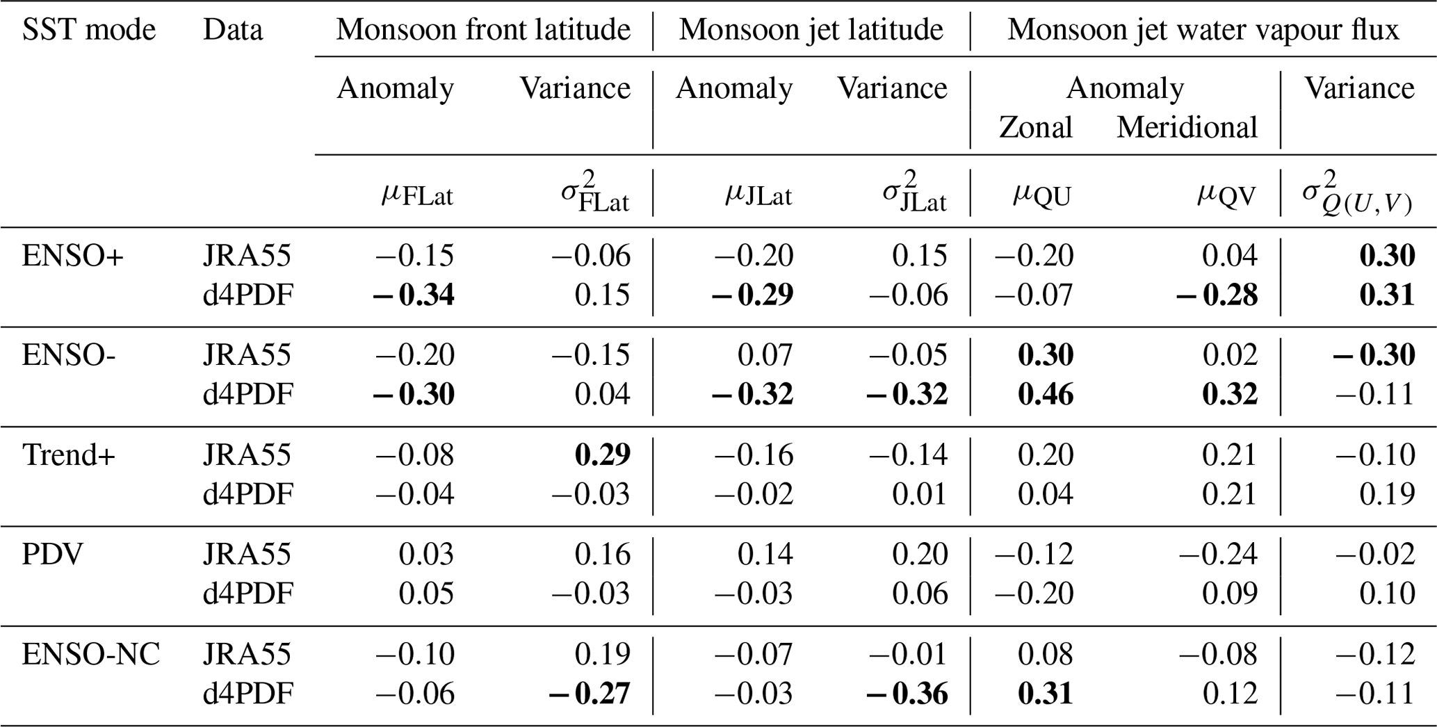
ENSO+ was significantly correlated with ${\mathit{\sigma }}_{Q(U,V)}^{\mathrm{2}}$ for both JRA55 (R = 0.30) and d4PDF (R = 0.31), from Table 2. There was significant anti-correlation only for d4PDF, with μ_QV ($R=-\mathrm{0.28}$), μ_JLat ($R=-\mathrm{0.29}$), and μ_FLat ($R=-\mathrm{0.34}$) but not for JRA55 (R=0.04, $R=-\mathrm{0.20}$, and $R=-\mathrm{0.15}$, respectively). The μ_JLat R values were similar between d4PDF and JRA55, but only d4PDF showed a spatially widespread relationship between μ_JLat and extreme rainfall (panels c vs. g for Figs. 13, 15, and 17), so μ_JLat was influential only for d4PDF; d4PDF displayed the stacked spatio-temporal signals of ${\mathit{\sigma }}_{Q(U,V)}^{\mathrm{2}}$ and reversed μ_JLat in the ENSO+ signals. Firstly, ENSO+ also showed weak correlation over eastern Kyushu only for hourly extremes but not otherwise (Fig. 7f vs. Figs. 8f and 9f), ${\mathit{\sigma }}_{Q(U,V)}^{\mathrm{2}}$ showed up to moderate correlation over eastern Kyushu only for hourly extremes but weak correlation otherwise (Fig. 14f vs. Figs. 16f and 18f), and reversed μ_JLat showed up to moderate correlation over Kyushu only for hourly extremes but weak correlation otherwise (reversed Fig. 13g vs. reversed Figs. 15g and 17g). Secondly, ENSO+ also showed weak correlation only for hourly and running-pentad extremes but not for daily extremes (Figs. 7f and 9f vs. Fig. 8f), ${\mathit{\sigma }}_{Q(U,V)}^{\mathrm{2}}$ showed weak correlation over Chugoku only for hourly and running-pentad extremes but not daily extremes (Figs. 14f and 18f vs. Fig. 16f), and reversed μ_JLat showed up to moderate correlation over Chugoku only for hourly and running-pentad extremes but weak correlation for daily extremes (reversed Figs. 13g and 17g vs. reversed Fig. 15g). The signals of reversed μ_QV, reversed μ_FLat, and the western Kyushu part of reversed μ_JLat seem to have cancelled out. Reversed μ_QV showed anti-correlation over western Kyushu and along the Sea of Japan coast (Figs. 14e, 16e, and 18e), reversed μ_FLat showed correlation along the Sea of Japan coast (Figs. 13e, 15e, and 17e), and reversed μ_JLat showed correlation over western Kyushu (Figs. 13g, 15g, and 17g). Reversed μ_QV showed correlation over Kanto (Figs. 14e, 16e, and 18e), and reversed μ_FLat showed anti-correlation over Kanto (Figs. 13g, 15g, and 17g). Unlike the stacking of signals with the same direction, it was more difficult to decide whether antagonising signals would cancel out. Two factors were involved: the strength of the relationship between SST modes and the regional monsoon and the strength of the relationship between the regional monsoon modes and extreme rainfall.

ENSO- was significantly correlated with μ_QU for both JRA55 (R=0.30) and d4PDF (R=0.46). There was significant correlation with μ_QV for d4PDF only (R=0.32) but not for JRA55 (R=0.02). There was significant anti-correlation with ${\mathit{\sigma }}_{Q(U,V)}^{\mathrm{2}}$ for JRA55 only ($R=-\mathrm{0.30}$) but not for d4PDF ($R=-\mathrm{0.11}$). There was significant anti-correlation for d4PDF with ${\mathit{\sigma }}_{\text{JLat}}^{\mathrm{2}}$ ($R=-\mathrm{0.32}$), μ_JLat ($R=-\mathrm{0.32}$), and μ_FLat ($R=-\mathrm{0.30}$) but not for JRA55 ($R=-\mathrm{0.05}$, R=0.07, and $R=-\mathrm{0.20}$, respectively). For observations, the stacking of correlation over southern Kyushu from μ_QU (Figs. 14a, 16a, and 18a) and reversed ${\mathit{\sigma }}_{Q(U,V)}^{\mathrm{2}}$ (Figs. 14c, 16c, and 18c) suggested that correlated rain gauges should be seen over southern Kyushu, but this was not the case (Figs. 7b, 8b, and 9b). However, stacking could explain d4PDF's excessive correlation between ENSO- and rainfall extremes. The three patterns of μ_QU (Figs. 14d, 16d, and 18d), μ_QV (Figs. 14e, 16e, and 18e), and reversed ${\mathit{\sigma }}_{\text{JLat}}^{\mathrm{2}}$ (reversed Figs. 13h, 15h, and 17h) were similar, with correlation along the Sea of Japan coast, correlation along the Pacific coast west of the topography, but anti-correlation along the Pacific coast east of the topography. Over western Japan, the anti-correlation was antagonised by the reversed μ_JLat signal of correlation (reversed Figs. 13g, 15g, and 17g). Over eastern Japan, particularly Kanto, the anti-correlation was antagonised by the reversed μ_FLat signal of correlation (reversed Figs. 13e, 15e, and 17e). This produced the d4PDF spatial pattern of correlation along the Sea of Japan coast and along the Pacific coast west of the topography but no relationship along the Pacific coast east of the topography (Figs. 7g, 8g, and 9g). A few moderately anti-correlated clusters were seen over Kanto for hourly extremes (Fig. 7g).

ENSO-NC showed only significant relationships with d4PDF. This was correlation with μ_QU (R=0.31 vs. JRA55 R=0.08), anti-correlation with ${\mathit{\sigma }}_{\text{JLat}}^{\mathrm{2}}$ ($R=-\mathrm{0.36}$ vs. JRA55 $R=-\mathrm{0.01}$), and anti-correlation with ${\mathit{\sigma }}_{\text{FLat}}^{\mathrm{2}}$ ($R=-\mathrm{0.27}$ vs. JRA55 R=0.19). Since ${\mathit{\sigma }}_{\text{FLat}}^{\mathrm{2}}$ was not influential for JRA55, the higher magnitude of R for JRA55 did not matter. The two patterns of μ_QU (Figs. 14d, 16d, and 18d) and reversed ${\mathit{\sigma }}_{\text{JLat}}^{\mathrm{2}}$ (reversed Figs. 13h, 15h, and 17h) were similar, as earlier described. This combined pattern stacked further with reversed ${\mathit{\sigma }}_{\text{FLat}}^{\mathrm{2}}$, which showed correlation over western Kyushu and anti-correlation along the Pacific coast of eastern Japan (reversed Figs. 13f, 15f, and 17f). This produced the d4PDF spatial pattern of correlation over western Kyushu and anti-correlation over eastern Japan (Figs. 7j, 8j, and 9j).

PDV showed no significant relationships with monsoon indices for either JRA55 or d4PDF. For JRA55, there were still two R values of stronger (but not significant) magnitude, with μ_QV ($R=-\mathrm{0.24}$ vs. d4PDF R=0.09) and ${\mathit{\sigma }}_{\text{JLat}}^{\mathrm{2}}$ (R=0.20 vs. d4PDF R=0.06). For d4PDF, there was only one R of stronger magnitude: μ_QU ($R=-\mathrm{0.20}$ vs. JRA55 $R=-\mathrm{0.12}$). Stacking could still explain the observed relationship between PDV and rainfall extremes, based on the spatio-temporal signals of ${\mathit{\sigma }}_{\text{JLat}}^{\mathrm{2}}$. Rain gauges showed a field-significant anti-correlation with PDV for daily extremes only (13 rain gauges; Fig. 8d) but not otherwise (Figs. 7d and 9d), with ${\mathit{\sigma }}_{\text{JLat}}^{\mathrm{2}}$ cluster-wise and gauge-wise field-significant anti-correlation for daily extremes (28 rain gauges and three clusters; Fig. 15d), gauge-wise field-significant anti-correlation for running-pentad extremes (15 rain gauges but only one cluster; Fig. 17d), and no field significance for hourly extremes (only 11 rain gauges and no clusters; Fig. 13d). Rain gauges showing anti-correlation with PDV were located over western Japan and Hokkaido (Fig. 8d); rain gauges showing anti-correlation with ${\mathit{\sigma }}_{\text{JLat}}^{\mathrm{2}}$ were located along the Pacific coast of western Japan (Fig. 15d), stacking with reversed μ_QV with anti-correlated rain gauges along the Sea of Japan coast of western Japan and over Hokkaido (Fig. 16b).

Trend+ showed only one statistically significant R among the regional monsoon indices, with ${\mathit{\sigma }}_{\text{FLat}}^{\mathrm{2}}$ for JRA55 (R=0.29 vs. d4PDF $R=-\mathrm{0.08}$). However, ${\mathit{\sigma }}_{\text{FLat}}^{\mathrm{2}}$ was not influential for JRA55. R values of stronger magnitude were with μ_QV for both JRA55 and d4DF (both R=0.21), with JRA55 only (R=0.20 vs. d4PDF R=0.04) and with d4PDF only (R=0.19 vs. JRA55 $R=-\mathrm{0.10}$). For observations, although μ_QU and μ_QV patterns might stack in terms of domain-wide correlation, the significantly correlated rain gauges were not co-located, with rain gauges for μ_QU and μ_QV concentrated along the Pacific coast and Sea of Japan coast, respectively. Furthermore, correlation with Trend+ was field significant only for hourly extremes (12 rain gauges; Fig. 6c), but correlation with μ_QU was best for daily extremes with cluster-wise and field significance (36 rain gauges and four clusters; Fig. 16a). For d4PDF, correlation with Trend+ was concentrated over Hokkaido and did not resemble the spatial patterns of μ_QV or ${\mathit{\sigma }}_{Q(U,V)}^{\mathrm{2}}$. Action through the regional monsoon front or regional monsoon jet does not seem to be a good mechanism to explain the influence of Trend+ on hourly rainfall extremes.

Finally, an explanation is proposed for why d4PDF showed stronger and spatially more widespread relationships between rainfall extremes and most of the regional monsoon indices. Considering the three most influential regional monsoon indices of μ_QU, μ_QV, and ${\mathit{\sigma }}_{\text{JLat}}^{\mathrm{2}}$, we observed that μ_QU and ${\mathit{\sigma }}_{\text{JLat}}^{\mathrm{2}}$ had reversed relationships with rainfall extremes for both observation and d4PDF. However, observed relationships were uniform, while d4PDF relationships were bipolar and showed strong topographic influence. This suggested that one reason could be the movement of the regional monsoon, with d4PDF having a more stable location that allowed topographic influences to strongly manifest.

Figure 20 shows the biweekly location of the regional monsoon for JRA55 and d4PDF. In early June, the monsoon was located at similar latitudes for both JRA55 and d4PDF, i.e. about to move into the study domain (Fig. 20a vs. Fig. 20e). In late June, the monsoon had moved over southern Kyushu for both JRA55 and d4PDF, but even at this time it was slightly more north for JRA55 where it passed over Kyushu (Fig. 20b vs. Fig. 20f). In early July, the JRA55 monsoon had passed over Kyushu and was over the Sea of Japan coast of western Japan (Fig. 20c). Over eastern Japan, it was south of the Pacific coast. In contrast, the d4PDF monsoon was still over northwest Kyushu and was between Chugoku and Shikoku island in western Japan (Fig. 20g). Over eastern Japan, it was along the Pacific coast. In late July, the JRA55 monsoon had reached the Korean Peninsula and was north of western Japan; it then moved diagonally southeast over eastern Japan into the Pacific (Fig. 20d). In contrast, the d4PDF monsoon still had a position similar to JRA55's early July position (Fig. 20h). It had a more zonal orientation extended further over eastern Japan, rather than off the coast as in JRA55. Hence, the d4PDF monsoon moved 2 weeks more slowly across the three large Japanese islands.

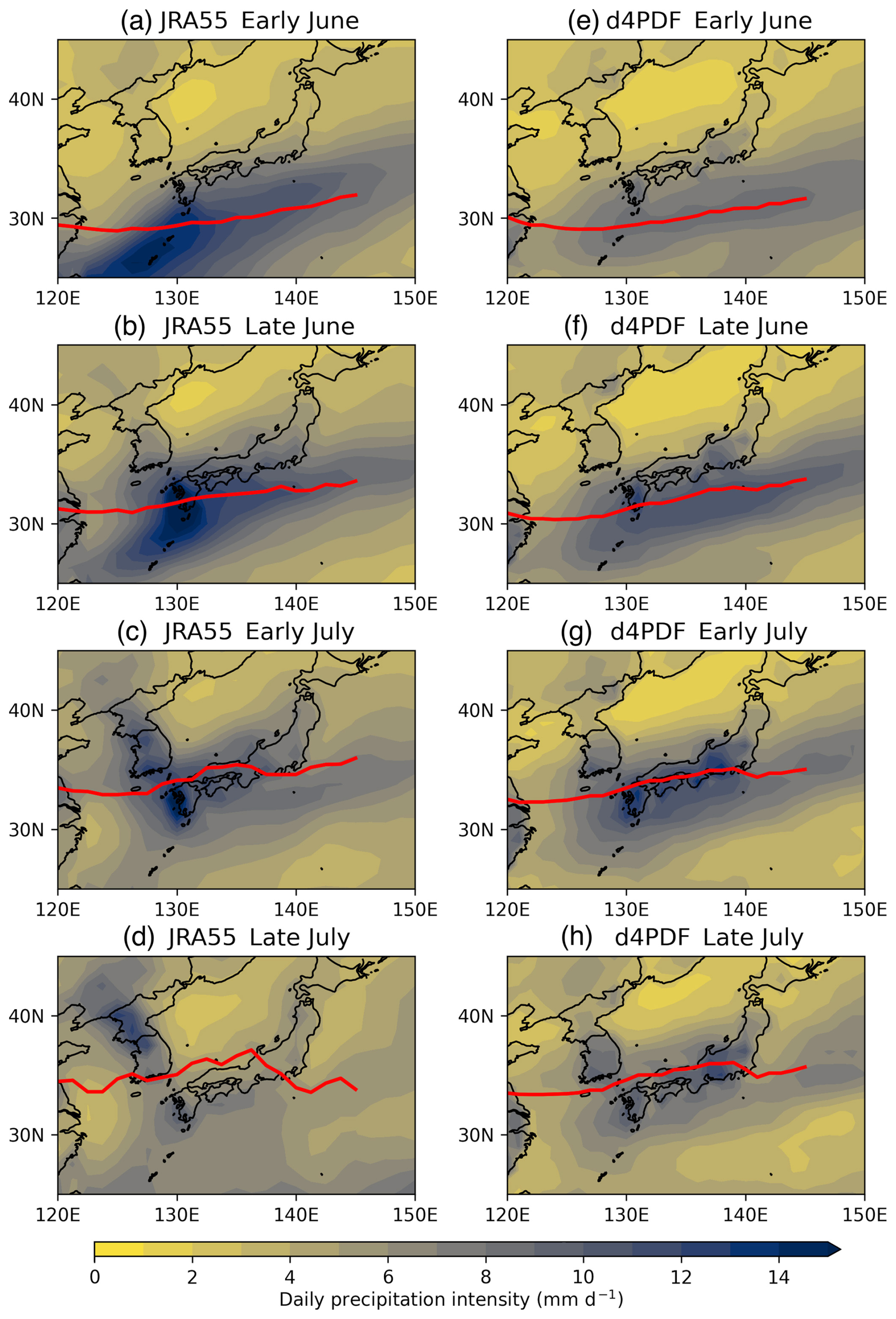
Figure 20 Monsoon front location (red line) and mean daily rainfall (in mm d⁻¹) (shading) for days when a continuous monsoon front could be detected, over four 2-week periods in June–July (rows), comparing JRA55 (a–d) and d4PDF (e–h). For JRA55, (a) first 2 weeks of June, (b) second 2 weeks of June, (c) first 2 weeks of July, and (d) second 2 weeks of July. For d4PDF, (e) first 2 weeks of June, (f) second 2 weeks of June, (g) first 2 weeks of July, and (h) second 2 weeks of July.

All other things being equal, the same synoptic disturbances travelling from the west would have a larger influence on the study domain in d4PDF, simply from the land regions of Japan capturing more rainfall from them in d4PDF. At least some of the differences between observation and d4PDF originated from the global model driving the regional model. This did not exclude other differences that might have originated from the regional model, but improvement of the monsoon movement in the global model would probably also improve extreme rainfall's global and regional teleconnections in d4PDF. The difference in monsoon position was quite minor, considering that it was only a regional spatio-temporal bias of about 2 weeks and 2° latitude in a global climate model. The difficulty to reproduce correct teleconnections is likely due to the unfortunate combination of a zonally aligned physical phenomenon with a zonally aligned geographically narrow island.

5 Conclusion

This study investigated the relationships between the June–July extreme rainfall over the four largest islands of Japan and the hemisphere-scale climate variability of SST anomalies over the Pacific basin. The 99th percentile hourly, 90th percentile daily, and 90th percentile running-pentad rainfall in the 59-year period of 1952–2010 was compared between d4PDF and rain gauges (observations). Observed extremes of each temporal resolution were independently clustered using the HDBSCAN algorithm based on their inter-location Spearman correlation. The multi-frequency extremes from the wavelet decomposition of hourly rainfall were then clustered based on a multi-frequency metric. Both methods produced similar clusters, and eight analysis regions were identified. The wavelet method was then applied to cluster d4PDF. Using each d4PDF set (cluster or unclassified point) as a spatial sample, Spearman correlation was calculated between the rainfall extremes and the standardised scores of five Pacific SST modes. The modes were obtained by the varimax rotation of extended principal component analysis on Pacific SST anomalies from COBE-SST2. Listed in order of explained variance for 1952–2010, they reflected canonical ENSO growth (ENSO+), canonical ENSO decay (ENSO-), warming trend mixed with other climate variability such as the NPGO (Trend+), a non-canonical ENSO that persisted into summer (ENSO-NC), and IPO-dominated Pacific decadal variability (PDV).

Observed and d4PDF correlation coefficients (R) were at most weak ($\left|R\right|<\mathrm{0.50}$) over most of Japan. Domain-wide field significance was observed between hourly extremes and Trend+ and between daily extremes and PDV. A group of rain gauges in northwest Kyushu were significantly related to ENSO+ for daily extremes, consistent with Kawamura et al. (2001) and Jin et al. (2005), which found strong rainfall over Fukuoka after strong La Niña events. In comparison, d4PDF was biased, showing excessive widespread correlation with ENSO- and excessive anti-correlation with ENSO-NC over eastern Japan. The observed PDV relationship was not reproduced. However, spatial correlation patterns for a smoothed Trend+ were similar between d4PDF and observations. Southern Kyushu showed stronger extremes for all three temporal resolutions.

Rainfall extremes were correlated with regional monsoon indices calculated from JRA55 and d4PDF-AGCM. Based on rain gauges and JRA55, μ_QU was the most influential index, with field correlation from 36 of 126 rain gauges showing significant correlation and up to moderate correlation for southern Kyushu. For both cases, the three most influential indices were the seasonal (June–July) anomaly of monsoon jet zonal water vapour flux (μ_QU), anomaly of monsoon jet meridional water vapour flux (μ_QV), and variance of monsoon jet latitude (${\mathit{\sigma }}_{\text{JLat}}^{\mathrm{2}}$). For both JRA55 and d4PDF, μ_QU was significantly correlated with ENSO-. For d4PDF, μ_QV was significantly correlated with ENSO- but anti-correlated with ENSO+. These relationships are consistent with Naoi et al. (2020), who found atmospheric rivers to be more frequent in years when El Niño transited into La Niña. An El Niño transitioning into a La Niña may be interpreted as combining the effects of the ENSO- mode with the reversed effects of the ENSO+ mode and hence associated with increased μ_QU (both cases) and μ_QV (d4PDF). The relationships between rainfall extremes and Pacific SST modes could be explained by the impact of the modes on the regional monsoon, in the form of water vapour flux modulation. The excessive relationships in d4PDF could be explained by the AGCM's slower latitudinal movement of the monsoon. The explanation was less successful at explaining the relationship between hourly extremes and the Trend+ mode.

Since SST anomalies rarely occur as pure modes but as a combination of modes, in a particular year a few climate modes may stack to create a stronger modulating effect on rainfall. Such cases would be exacerbated by the influence of the Trend+ mode in the future warmer climate, specifically the strengthening of hourly extremes (Fig. 5c). The statistical results of this study should be further investigated through sensitivity tests using physics-based numerical weather prediction models. Recently, large ensemble climate prediction datasets such as d4PDF have been widely used in order to extract probabilities of occurrence of extreme weather such as tropical cyclones and heavy rainfalls. Attributing of such extreme events to global warming has been one of the foci in climate and impact assessment studies. In identifying the relationship of extreme events with specific climate modes, special care in evaluating the representation and performance of climate prediction datasets is desirable. This study demonstrates one of the approaches for such evaluations.