Consistency between a strain rate model and the ESHM20 earthquake rate forecast in Europe: insights for seismic hazard

This work aims at investigating the consistency between a strain rate model and a long-term earthquake forecast at the European scale. We take advantage of the release of geodetic strain rate models by Piña-Valdés et al. (2022) and the release of the European Seismic Hazard Model 2020 (ESHM20) by Danciu et al. (2024) to compare geodetic and seismic moment rates across Europe. Seismic moments are inferred from the magnitude–frequency distributions that constitute the ESHM20 source model. We explore the full ESHM20 source model logic tree to account for epistemic uncertainties. On the geodesy side, we use the strain rates to calculate the geodetic moment for each area source zone of the hazard model, considering associated epistemic uncertainties. We show that the parameters contributing the most to the overall uncertainty in the geodetic moment rate are the distance weighting scheme used in the spatial inversion, the equation used to convert surface strain to a scalar moment rate, and the effective seismic thickness. We compare the distributions of geodetic and seismic moment rates at different geographical scales. In highly seismic activity zones, such as the Apennines in Italy, Greece, the Balkans, and the Betics in Spain, primary compatibility between seismic and geodetic moment rates is evident. Discrepancies emerge in low- to moderate-seismic-activity zones, particularly in areas affected by the Scandinavian glacial isostatic adjustment, where geodetic moment rates exceed seismic moment rates significantly. We show that considering broader zones enhances the match between geodetic and seismic moment rate distributions. In zones where ESHM20 magnitude–frequency distributions are well-constrained (established on more than 30 complete events), the distributions of seismic and geodetic moments usually overlap significantly, suggesting the potential for integrating geodetic data into hazard models, even in regions with low deformation.

1 Introduction

Nowadays, source models in up-to-date probabilistic seismic hazard assessment (PSHA) studies are based on both past seismicity and active tectonic datasets. For example, the source model logic trees in the European Seismic Hazard Model 2013 (Woessner et al., 2015) and in the updated European Seismic Hazard Model 2020 (Danciu et al., 2024) include two main branches, an area source model and a fault model. In regions where active faults are rather well-characterized, they must be accounted for in the hazard estimations (e.g., Stirling et al., 2012; Field et al., 2014; Beauval et al., 2018). Fault models are mostly based on geologic information, covering much larger time windows than the available earthquake catalogs, and bring insights into the generation of earthquakes that complement the catalog-based earthquake forecasts. However, fault databases are known to be incomplete, even in the best-characterized regions, and earthquakes may occur on unknown faults, as demonstrated by several earthquakes in the past, such as the two 2002 M_w ≈ 5.7 Molise earthquakes (Valensise et al., 2004) in Italy or the Darfield M_w 7.1 earthquake in Aotearoa / New Zealand (Hornblow et al., 2014).

A number of studies have analyzed the relationship between geodetic strain rates and observed seismicity (e.g., Zeng et al., 2018; Kreemer and Young, 2022; Riguzzi et al., 2012; Farolfi et al., 2020). However, the use of geodetic data in the development of source models for PSHA has been limited up to now, although deformation rates based on velocities from the Global Navigation Satellite Systems (GNSS) constitute a promising perspective for constraining earthquake recurrence models (Jenny et al., 2004; Shen et al., 2007). GNSS stations measure the present-day displacements at the surface of the earth. A convenient way to characterize the ground deformation is to invert the surface velocities measured by GNSS to compute strain rate maps, which are independent of the reference frame. The accuracy of the estimated strain rates depends on the spatial density of GNSS stations, the quality of the sites, and the duration of the records (Mathey et al., 2018). Along major interplate faults, such as subduction zones or lithospheric strike-slip faults, interseismic velocities measured by GNSS are now commonly used to constrain the slip deficit on the fault associated with locking in between large seismic events, also referred to as interseismic coupling. In such highly active tectonic boundary regions, the interseismic slip deficit may be combined with the earthquake catalog to constrain earthquake recurrence (Avouac, 2015; Mariniere et al., 2021). In plate interiors, where the faults move at low slip rates and where fault mapping is incomplete, strain rate models can provide constraints on the seismic potential.

Indeed, the tectonic loading recorded by geodesy should be proportional to the energy released during earthquakes, under the assumption that the earth's crust behaves elastically (Reid, 1910). If this assumption is true and other factors such as aseismic deformation are not significant, then the rate at which energy is released during earthquakes (represented by the seismic moment rate) and the rate at which tectonic forces build up between earthquakes (represented by the geodetic moment rates) should be equal (Stevens and Avouac, 2021). This balance can be used to constrain magnitude–frequency distributions. In the last 30 years, a number of studies have analyzed catalog-based magnitude–frequency distributions with respect to the tectonic loading measured by geodesy. Based on the mapping of strain rates from geodesy in the Hellenic Arc, Jenny et al. (2004) found that the maximum magnitudes required for the earthquake recurrence models to be moment balanced were unrealistic and concluded that a large part of the strain is released in aseismic processes, following Papadopoulos (1989). In the India–Asia collision zone, Stevens and Avouac (2021) highlighted a correlation between earthquake rates and strain rates. They established moment-balanced recurrence models that fit both past seismicity and the geodetic moment, bounded by maximum magnitudes compatible with those expected in the region. They combine these moment-balanced earthquake recurrence models with ground-motion models to estimate probabilistic seismic hazard (e.g., Stevens and Avouac, 2021).

However, to our knowledge, in Europe, the only seismic hazard model that integrates a source model based on strain rates is the new Italian hazard model (Meletti et al., 2021). The gridded-seismicity model MG1 (Visini et al., 2021) relies on a strain rate tensor field calculated using velocity interpolation for strain rate (VISR) software (Shen et al., 2015), similar to Piña-Valdés et al. (2022). The rate of the seismic moment is converted into earthquake rates assuming that earthquakes are distributed according to a tapered Gutenberg–Richter, considering two alternative seismogenic thicknesses (7 and 13 km). The total seismic rate is scaled to the seismic moment release of the Italian catalog (Visini et al., 2021). Meletti et al. (2021) also include a second more complex geodetically based source model, MG2. In this case, the model relies on NeoKinema code (Bird, 2009) that delivers interseismic and long-term strain rates and velocities on a finite-element grid (see Bird and Carafa, 2016).

Determining the extent to which the methods used to study highly active tectonic regions can be applied to areas with lower levels of seismic activity is an open research question. The present study is at the scale of the whole European continent, which is very heterogeneous in terms of tectonic activity. Southern Europe, with regions such as the Apennines, Greece, and Türkiye, is characterized by high seismic activity and significant tectonic deformation (Nocquet, 2012; de Vicente and Vegas, 2009), whereas northern and central Europe is characterized by low to moderate seismic activity (Kierulf et al., 2021; Lukk et al., 2019). We take advantage of two new studies performed at the scale of Europe: the release of the new probabilistic seismic hazard model for Europe (ESHM20, Danciu et al., 2024) and the strain rate models computed by Piña-Valdés et al. (2022), as presented in Fig. 1. Our objective is to compare the ESHM20 earthquake rate forecast with the deformation rates obtained from the GNSS velocities, giving special attention to the estimation of uncertainties.

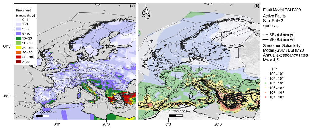
Figure 1 Strain rate model for Europe and ESHM20 earthquake rate forecast (smoothed seismicity and fault model branch). (a) II invariant of the strain rate tensor (Piña-Valdés et al., 2022) with area sources of ESHM20 superimposed. (b) Smoothed seismicity model with earthquake rates of M_W ≥ 4.5; faults included in the model are superimposed (Danciu et al., 2021a, 2024).

In a first step, we present the datasets and methods used to compute the seismic and geodetic moment rate distributions. Next, we compare the obtained seismic and geodetic moment rate distributions at the scale of the ESHM20 area source zones. We then discuss the parameters that most influence the compatibility in high- and low- to moderate-seismicity regions.

2 Methods and data

2.1 Seismic moment: moment distributions associated with the ESHM20 source model logic tree

ESHM20 aimed at delivering seismic hazard levels throughout Europe, using harmonized datasets and applying homogeneous methodologies (Danciu et al., 2024). The hazard model consists of two main components: a seismogenic source model forecasting earthquakes in space, time, and magnitude and a ground-motion model predicting the ground motions these earthquakes may generate. The present study deals with the seismogenic source model. The earthquake rate forecast includes all earthquake types, i.e., crustal, deep (Vrancea region, Romania), and subduction (Hellenic, Cyprian, Calabrian, and Gibraltar arcs) earthquakes. In this paper we focus on the contribution of crustal shallow seismogenic sources, which can be directly compared to surface strain rate.

ESHM20's seismogenic source model is based on several updated datasets (Danciu et al., 2021a, 2024): an earthquake catalog, covering the time window 1000–2014, including both historical (Rovida et al., 2022) and instrumental (Lammers et al., 2023) periods, and a fault database including potentially active faults, with their geometry and geologic or geodetic slip rates (European Fault-Source Model 2020 (EFSM20); Basili et al., 2024). The source model logic tree accounts for alternative source models to capture the spatial and temporal variability of the earthquake rate forecast in Europe. It includes two main branches: an area source model and a hybrid model that combines active faults with a background smoothed seismicity model (Danciu et al., 2021a).

The area source model consists of cross-border harmonized seismogenic sources whose geometry is guided by seismotectonic evidence, such as potentially active faults, geologic features, and seismicity patterns (Danciu et al., 2021a, 2024). For each area source, a Gutenberg–Richter magnitude–frequency distribution (Gutenberg and Richter, 1944) has been evaluated from the earthquake catalog taking into account time windows of completeness. Two alternative models have been considered to account for the uncertainty in forecasting earthquake rates in the upper-magnitude range:

• The first is a magnitude–frequency distribution truncated at a maximum magnitude M_max, corresponding to Form 2 in Anderson and Luco (1983):

  $$\begin{array}{}\text{(1)}& N\left(m\right)={\mathrm{10}}^{a-b\times m}+{\mathrm{10}}^{a-b{M}_{\max }}\text{for}m\le M_{\max },\end{array}$$

  where N(m) represents the cumulative annual rate of events as a function of magnitude (m); a and b are the Gutenberg–Richter recurrence coefficients, namely the productivity and the exponential coefficient, respectively; and M_max is the maximum magnitude.

• The second is a tapered Pareto distribution (Kagan, 2002), which includes a bending of the recurrence model from a magnitude called the corner magnitude (M_c). With respect to the Anderson and Luco (1983) magnitude–frequency distribution, the sharp cutoff at a maximum magnitude in the truncated distribution is replaced by smooth tapering.

An alternative to the area source model is the hybrid model, consisting of active crustal faults combined with off-fault smoothed seismicity (Fig. 2). For each fault, a moment-balanced magnitude–frequency distribution has been established, which accommodates the moment inferred from the slip rate and the geometry of the fault, assuming the moment conservation principle. The maximum magnitude is obtained applying the Leonard (2010, 2014) scaling relationships to the length, the width, and the area of the fault (Basili et al., 2024). The smoothed seismicity model is built from the earthquake catalog and forecast earthquake rates within spatial cells, using a grid with 0.1° spacing. This smoothed seismicity model is developed by optimizing the adaptive kernel bandwidth, the smoothing parameters, and the declustering parameters. Training and validation sets are used to determine the optimal combination of parameters. To avoid double counting, a buffer zone is applied around each fault. Details are provided in the EFEHR (European Facilities of Earthquake Hazard and Risk) report (see Danciu et al., 2021a).

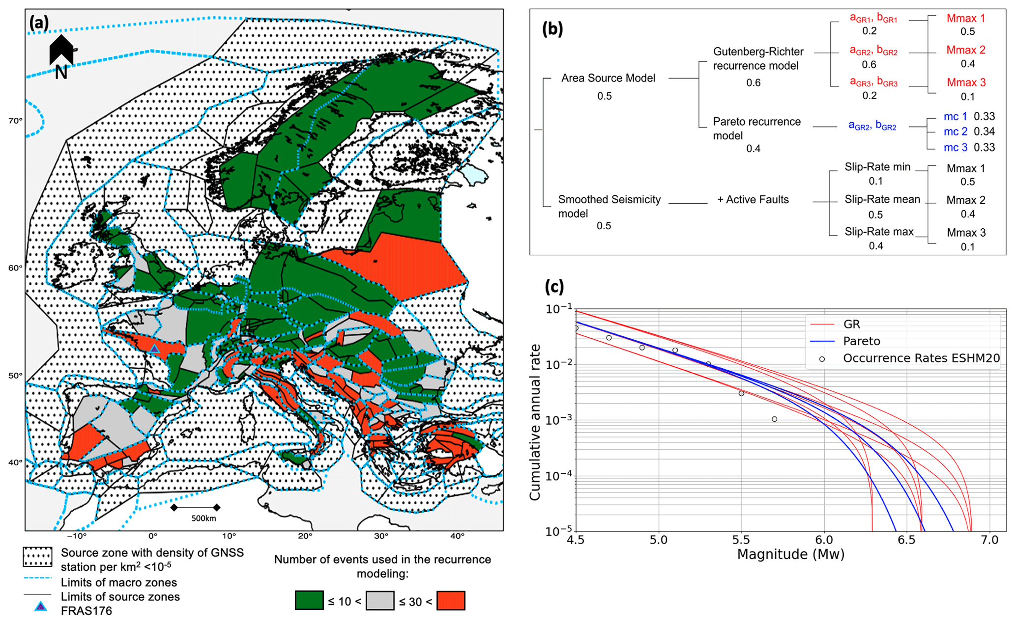
Figure 2 ESHM20 source model (Danciu et al., 2024): (a) area sources (black polygons) and larger macrozones (dashed blue) used to infer the b value in regions with poor earthquake data; orange – sources with at least 30 events used to establish the recurrence model, green – sources with less than 10 events, black dots – area sources not considered in the study (poorly constrained strain rates). (b) Source model logic tree, with the weights associated with the different branches. (c) Alternative earthquake recurrence models for the example source zone FRAS176 (southern Brittany in France, blue triangle); colors correspond to the branch combinations in the area source model (b). Area source zone polygons can also be found in Fig. 6.

The source model logic tree explores the uncertainty in the definition of the maximum (or corner) magnitude, both in the area source model and in the fault model (Fig. 2). For the area source model, the uncertainty in the estimation of a and b values is also considered (Gutenberg–Richter model branch). For the fault model, the uncertainty in the slip rate estimates is explored. Overall, the exploration of the logic tree leads to 21 alternative recurrence models, with different weights.

For every area source zone, 21 alternative estimates for the seismic moment are computed from the 21 alternative magnitude–frequency distributions. Considering the Gutenberg–Richter and Pareto recurrence models, the total annual moment rate corresponds to the integral under the curve in terms of moment. In the case of the Gutenberg–Richter model (Form 2 in Anderson and Luco, 1983), the following equation is used (Mariniere et al., 2021):

$$\begin{array}{}\text{(2)}& {\dot{M}}_{\mathrm{0}\mathrm{S}}={\displaystyle \frac{b}{(c-b)}}\times {\mathrm{10}}^{a+d+(c-b)M_{\max }},\end{array}$$

in N m yr⁻¹, with c = 1.5 and d = 9.1 being the parameters used in the calculation of the seismic moment from the moment magnitude (Hanks and Kanamori, 1979).

To compute the annual seismic moment rate from the smoothed seismicity and fault model, we sum the seismic moments associated with every spatial cell within the area source zone (one magnitude–frequency distribution per cell). When a fault straddles several zones, the seismic moment associated with the source zone is proportional to the length of the fault within the source zone.

For each source zone, a distribution of 21 seismic moments is obtained, representative of the uncertainties considered in the ESHM20 seismogenic source logic tree. A weighted mean seismic moment is calculated considering the weights associated with every branch combination (Fig. 2). Moreover, approximate 16th and 84th percentiles are inferred from the discrete distributions.

2.2 Geodetic moment computation from strain rate maps and uncertainty exploration

Our aim is to use the strain rates to estimate the geodetic moment rates within every area source of the ESHM20 source model. To achieve this goal, we start from the work of Piña-Valdés et al. (2022). They combined 10 GNSS velocity fields with different spatial coverage in Europe. After filtering the velocity field to remove stations with the highest uncertainties, they applied the VISR algorithm (Shen et al., 2015) to derive a strain rate model for Europe (a best-estimate model). The VISR algorithm calculates horizontal strains through interpolation of a geodetic velocity field. It is an undetermined inverse problem: the algorithm uses the discretized geodetic observations as inputs and delivers smoothed distributed strain rates. Key decisions need to be taken on the exact weighting scheme to apply, which may impact the interpolation and the final strain rate estimates. In our case, rather than a best estimate, we need a distribution for the geodetic moment rate that is representative of the uncertainties.

2.2.1 Uncertainties in the strain rate estimates

Ideally, only the stations with the best-constrained velocity estimates should be included for deriving strain rates. However a compromise must be obtained between discarding poorly constrained stations and keeping a reasonable number of stations for the analysis. Piña-Valdés et al. (2022) have classified the 4863 available stations into four categories, i.e., A, B, C, and remaining stations, depending on their noise level responsible for the uncertainty in the velocity (the noise and the uncertainty in the velocity increase from the class A station ahead). To derive their best model, they decided to include all stations falling into categories A, B, and C. Here, we are interested in quantifying how much this decision impacts the strain rate estimates, and we explore the uncertainty related to the use of only class A stations (3377); both A and B stations (4091); and stations A, B, and C (4468).

For the strain rates to be reliable, anomalous velocities must be identified and removed from the combined velocity field. Piña-Valdés et al. (2022) proposed detecting outliers based on an analysis of the spatial consistency of the velocities. For every station, the distribution of the velocities within a circular region around the station is obtained; stations with velocities in the tails of the distribution are considered outliers. Piña-Valdés et al. (2022) tested four different radii (50, 100, 150, and 200 km) and showed that when the radius increases, the number of outliers decreases. They used 150 km for deriving their best-estimate model, considering this radius is a compromise between the number of stations left (4238) and a reduction in the variance obtained on the final solution. Here, we keep track of the uncertainty associated with this decision, and we alternatively use the four different radii to evaluate strain rates.

While applying the VISR algorithm, a number of required decisions may impact horizontal strain rate estimates: the distance and spatial weighting scheme and the weighting threshold implied in the spatial inversion. Shen et al. (2015) show that the distance-dependent weighting can be achieved by employing either a Gaussian or a quadratic decay function and that for the spatially dependent weighting, either an azimuthal weighting or a Voronoi cell area weighting function can be applied. Another crucial parameter is the weighting threshold, which governs the smoothing of the inversion process. Here we include in the analysis the uncertainty in both the smoothing function and the spatially dependent weighting, as well as three alternative weighting threshold values (6, 12, and 24; see Shen et al., 2015).

2.2.2 Estimation of the geodetic moment rate within an area source zone

For each area source of the ESHM20 model, we determine a distribution for the geodetic moment rate. Figure 3 illustrates the different steps for the source zones in northwestern France.

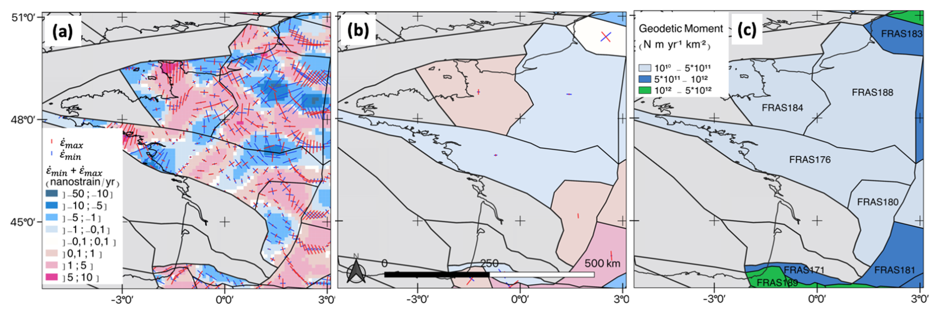
Figure 3 Scalar geodetic moment computed from a mean strain tensor, with an example for the source zones in northwestern France. (a) Horizontal strain rate tensor from the best model of Piña-Valdés et al. (2022), for each grid cell: principal components of the strain rate tensor (${\dot{\mathit{\epsilon }}}_{\min }$ in red; ${\dot{\mathit{\epsilon }}}_{\max }$ in blue) and deformation style (${\dot{\mathit{\epsilon }}}_{\min }+{\dot{\mathit{\epsilon }}}_{\max }$; red: extension, blue: compression). (b) Mean strain rate tensor per source zone and mean principal components in the source zone (${\stackrel{\mathrm{‾}}{\dot{\mathit{\epsilon }}}}_{\min }$ and ${\stackrel{\mathrm{‾}}{\dot{\mathit{\epsilon }}}}_{\max }$) (Eqs. 4, 5). (c) One estimate for the geodetic moment rate within the source zone, using the best model from Piña-Valdés et al. (2022) and considering a depth of 10 km, a shear modulus of $\mathit{\mu }=\mathrm{3.3}\times {\mathrm{10}}^{\mathrm{10}}$ N m⁻², the equation from Savage and Simpson (1997), and a geometric coefficient C_g equal to 2. Abbreviations of ESHM20 area source zones are indicated.

First, for each component of the strain rate tensor (${\dot{\mathit{\epsilon }}}_{xx}$, ${\dot{\mathit{\epsilon }}}_{yy}$, ${\dot{\mathit{\epsilon }}}_{xy}$), we determine the mean component from all grid cells falling within the source zone (Fig. 3a and b):

$$\begin{array}{}\text{(3)}& {\stackrel{\mathrm{‾}}{{\dot{\mathit{\epsilon }}}_{xx}}}^{\mathrm{2}}={\displaystyle \frac{{\sum }_{i=\mathrm{1}}^{\mathrm{ncells}}{\dot{\mathit{\epsilon }}}_{xx}\left(i\right)}{\text{ncells}}},\end{array}$$

with ncells being the number of cells considered.

Then we calculate the principal components (eigenvalues) of the strain rate tensor within the area source:

$$\begin{array}{}\text{(4)}& \begin{array}{rl}& \stackrel{\mathrm{‾}}{{\dot{\mathit{\epsilon }}}_{\max }}=\text{MAX}\left({\displaystyle \frac{{\stackrel{\mathrm{‾}}{\dot{\mathit{\epsilon }}}}_{xx}+\stackrel{\mathrm{‾}}{{\dot{\mathit{\epsilon }}}_{yy}}}{\mathrm{2}}}\right.+\sqrt{({\displaystyle \frac{\stackrel{\mathrm{‾}}{{\dot{\mathit{\epsilon }}}_{xx}}-\stackrel{\mathrm{‾}}{{\dot{\mathit{\epsilon }}}_{yy}}}{\mathrm{2}}}{)}^{\mathrm{2}}+{\stackrel{\mathrm{‾}}{{\dot{\mathit{\epsilon }}}_{xy}}}^{\mathrm{2}}},\\ & {\displaystyle \frac{\stackrel{\mathrm{‾}}{{\dot{\mathit{\epsilon }}}_{xx}}+\stackrel{\mathrm{‾}}{{\dot{\mathit{\epsilon }}}_{yy}}}{\mathrm{2}}}-\left.\sqrt{({\displaystyle \frac{\stackrel{\mathrm{‾}}{{\dot{\mathit{\epsilon }}}_{xx}}-\stackrel{\mathrm{‾}}{{\dot{\mathit{\epsilon }}}_{yy}}}{\mathrm{2}}}{)}^{\mathrm{2}}+{\stackrel{\mathrm{‾}}{{\dot{\mathit{\epsilon }}}_{xy}}}^{\mathrm{2}}}\right),\end{array}\end{array}$$

$$\begin{array}{}\text{(5)}& \begin{array}{rl}& \stackrel{\mathrm{‾}}{{\dot{\mathit{\epsilon }}}_{\min }}=\text{MIN}\left({\displaystyle \frac{{\stackrel{\mathrm{‾}}{\dot{\mathit{\epsilon }}}}_{xx}+\stackrel{\mathrm{‾}}{{\dot{\mathit{\epsilon }}}_{yy}}}{\mathrm{2}}}\right.+\sqrt{({\displaystyle \frac{\stackrel{\mathrm{‾}}{{\dot{\mathit{\epsilon }}}_{xx}}-\stackrel{\mathrm{‾}}{{\dot{\mathit{\epsilon }}}_{yy}}}{\mathrm{2}}}{)}^{\mathrm{2}}+{\stackrel{\mathrm{‾}}{{\dot{\mathit{\epsilon }}}_{xy}}}^{\mathrm{2}}},\\ & {\displaystyle \frac{\stackrel{\mathrm{‾}}{{\dot{\mathit{\epsilon }}}_{xx}}+\stackrel{\mathrm{‾}}{{\dot{\mathit{\epsilon }}}_{yy}}}{\mathrm{2}}}-\left.\sqrt{({\displaystyle \frac{\stackrel{\mathrm{‾}}{{\dot{\mathit{\epsilon }}}_{xx}}-\stackrel{\mathrm{‾}}{{\dot{\mathit{\epsilon }}}_{yy}}}{\mathrm{2}}}{)}^{\mathrm{2}}+{\stackrel{\mathrm{‾}}{{\dot{\mathit{\epsilon }}}_{xy}}}^{\mathrm{2}}}\right).\end{array}\end{array}$$

As underlined by previous authors (e.g., Ward, 1998; Pancha, 2006), the conversion of surface strain to a scalar moment rate bears large uncertainties, and there is no unique method. We use three different equations for calculating the moment rate to propagate this uncertainty up to the final moment rate estimate:

• The Working Group on California Earthquake Probabilities (1995) uses the difference between the principal strain rates:

  $$\begin{array}{}\text{(6)}& {\dot{M}}_{\mathrm{0}\mathrm{G}}=\mathrm{2}\mathit{\mu }AH(\stackrel{\mathrm{‾}}{{\dot{\mathit{\epsilon }}}_{\max }}-\stackrel{\mathrm{‾}}{{\dot{\mathit{\epsilon }}}_{\min }}).\end{array}$$

• Savage and Simpson (1997) propose that the scalar moment rate is at least as large as

  $$\begin{array}{}\text{(7)}& {\dot{M}}_{\mathrm{0}\mathrm{G}}=\mathrm{2}\mathit{\mu }AH\text{MAX}\left(\right|\stackrel{\mathrm{‾}}{{\dot{\mathit{\epsilon }}}_{\max }}|,|\stackrel{\mathrm{‾}}{{\dot{\mathit{\epsilon }}}_{\min }}|,|\stackrel{\mathrm{‾}}{{\dot{\mathit{\epsilon }}}_{\max }}-\stackrel{\mathrm{‾}}{{\dot{\mathit{\epsilon }}}_{\min }}\left|\right).\end{array}$$

• Stevens and Avouac (2021) use the second invariant, which reflects the magnitude of the total strain rate:

  $$\begin{array}{}\text{(8)}& {\dot{M}}_{\mathrm{0}\mathrm{G}}=C_{\mathrm{g}}\mathit{\mu }AH\sqrt{{\stackrel{\mathrm{‾}}{{\dot{\mathit{\epsilon }}}_{xx}}}^{\mathrm{2}}+{\stackrel{\mathrm{‾}}{{\dot{\mathit{\epsilon }}}_{yy}}}^{\mathrm{2}}+\mathrm{2}{\stackrel{\mathrm{‾}}{{\dot{\mathit{\epsilon }}}_{xy}}}^{\mathrm{2}}}.\end{array}$$

Here, A is the area of the zone, μ is the shear modulus, and H is the seismogenic thickness. C_g is a geometric coefficient, which depends on the orientation and dip angle (δ) of the fault plane accommodating the strain. Following Stevens and Avouac (2021), for dip-slip faults with uniaxial compression, $C_{\mathrm{g}}=\mathrm{1}/\left[\sin \left(\mathit{\delta }\right)\cdot \cos \left(\mathit{\delta }\right)\right]$. A dip of 45° corresponds to a geometric coefficient equal to 2, which is the value assumed by the Working Group on California Earthquake Probabilities (1995) and Savage and Simpson (1997), as well as in a large part of the literature (e.g., Ward, 1998; Jenny et al., 2004; Bird and Liu, 2007; D'Agostino, 2014). In their study on the Himalayan region, Stevens and Avouac (2021) consider two values of C_g, corresponding to dips between 45° (C_g = 2) and 15° (C_g = 4), to account for the low-angle thrust faults in the region. Here we consider two C_g values, 2 and 2.6, which is the range corresponding to a dip between 25 and 65°, representing standard thrust and normal faults, respectively.

The uncertainty in the shear modulus is also taken into account, including two alternative values proposed for continental crust: 3.3×10¹⁰ and 3.0×10¹⁰ N m⁻² (e.g., Dziewonski and Anderson, 1981; Burov, 2011), and is widely used in the literature (e.g., Stevens and Avouac, 2021; Working Group on California Earthquake Probabilities, 1995; Mazzotti and Adams, 2005). For the seismogenic thickness (H in Eqs. 6 to 8), we consider here the elastic thickness, i.e., the average thickness over which a region's principal faults store and release seismic energy (Ward, 1998). Only a fraction of the frictional slip takes place during earthquakes (Bird et al., 2002). Mazzotti and Adams (2005) define the “effective seismic thickness” as the thickness of the crust where deformation is fully accommodated by seismicity. In an application in eastern North America, they show that this effective seismic thickness may represent only 40 % of the seismogenic thickness based on maximum and minimum depths of earthquakes. The thickness considered in the literature to evaluate seismic moment release from strain rates usually varies between 5 and 15 km. Pancha (2006) used a fixed seismogenic thickness of 15 km throughout the Basin and Range regions in the western US. D'Agostino (2014) applied a thickness of 10 ± 2.5 km throughout the Apennines in Italy. Stevens and Avouac (2021) considered 15 km in the India–Asia collision zone. Carafa et al. (2017) estimated average coupled thicknesses between 3 and 8 km for faults in Italy. At last, using strain rates to forecast earthquakes in the Italian seismic hazard model, Visini et al. (2021) assume elastic thickness equal to 7 and 13 km throughout Italy. As there is considerable uncertainty in this parameter, based on this literature review, we use three alternative values (5, 10, and 15 km) and propagate this uncertainty up to the geodetic moment rate estimates.

2.2.3 A geodetic moment rate distribution per area source zone

The aim is to obtain a distribution of the moment rate within an area source of ESHM20 that is representative of the uncertainties. Figure 4 displays the exploration tree set up to combine 12 different preprocessing parameters to filter the stations of the GNSS velocity fields (three selections of GPS station times, four outlier radii) with 12 different regularizations of the velocity field inversion to determine strain rates (choice of the distance and spatial weighting scheme, choice of the weighting threshold) and, finally, with 36 different parameterizations to calculate the moment rate from the strain rates. For a given source zone area, we obtain 5184 alternative moment rate estimates ($\mathrm{12}\times \mathrm{12}\times \mathrm{36}$). Figure 4b displays the distribution obtained for the example area source zone hosting Paris in France. The variability of the moment rate is significant – the value corresponding to the 84th percentile is 3 times larger than the value corresponding to the 16th percentile.

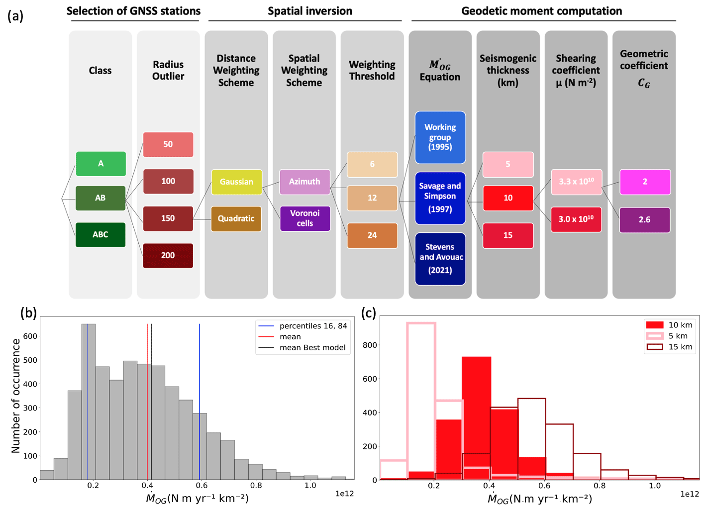
Figure 4 Determination of a distribution for the moment rate per area source zone, taking into account the uncertainties in the different steps. (a) Exploration tree to account for the uncertainty in the exact set of GNSS stations used, the technique applied to infer strain rates from the geodetic velocities, and the parameters used to calculate the moment rate within an area source. Exploration of the full tree results in $\mathrm{3}\times \mathrm{4}\times \mathrm{2}\times \mathrm{2}\times \mathrm{3}\times \mathrm{3}\times \mathrm{3}\times \mathrm{2}\times \mathrm{2}$ = 5184 alternative moment rate estimates. (b) Distribution of the geodetic moment rate estimates (histogram built from the 5184 values) obtained for the example source zone, namely the Parisian Basin in France (FRAS188 in ESHM20); the mean value (red); and the 16th and 84th percentiles (blue). (c) Three alternative distributions for the moment rate estimates, depending on the choice of the seismogenic depth, for the Parisian Basin example source zone in France.

To understand which parameters, or decisions, mostly control the overall variability in the geodetic moment, different parts of the tree are explored (Fig. 5; see Mariniere et al., 2021). The analysis is displayed in three example area source zones characterized by different seismic activity: southern Brittany in France, located in an intracontinental region and characterized by low seismic activity; a large source zone in Fennoscandia in a very low seismicity region; and northern Tuscany in Italy, a moderate-seismicity region (see Fig. 6 for locations). For every parameter choice, the entire tree is explored, keeping fixed the other parameters, then, from the distribution obtained, the mean and the 16th and 84th percentiles are estimated. For example, exploring the alternative branches corresponding to the three different selections of GPS stations separately yields three distributions, made of 1728 moment estimates each (in green). Exploring the branches based on the two alternative spatial weighting schemes separately yields two alternative distributions, made of 2592 moment estimates each (in purple). The larger the dispersion obtained between the alternative mean values of the distributions, the larger is the contribution of this parameter uncertainty to the overall moment rate variability.

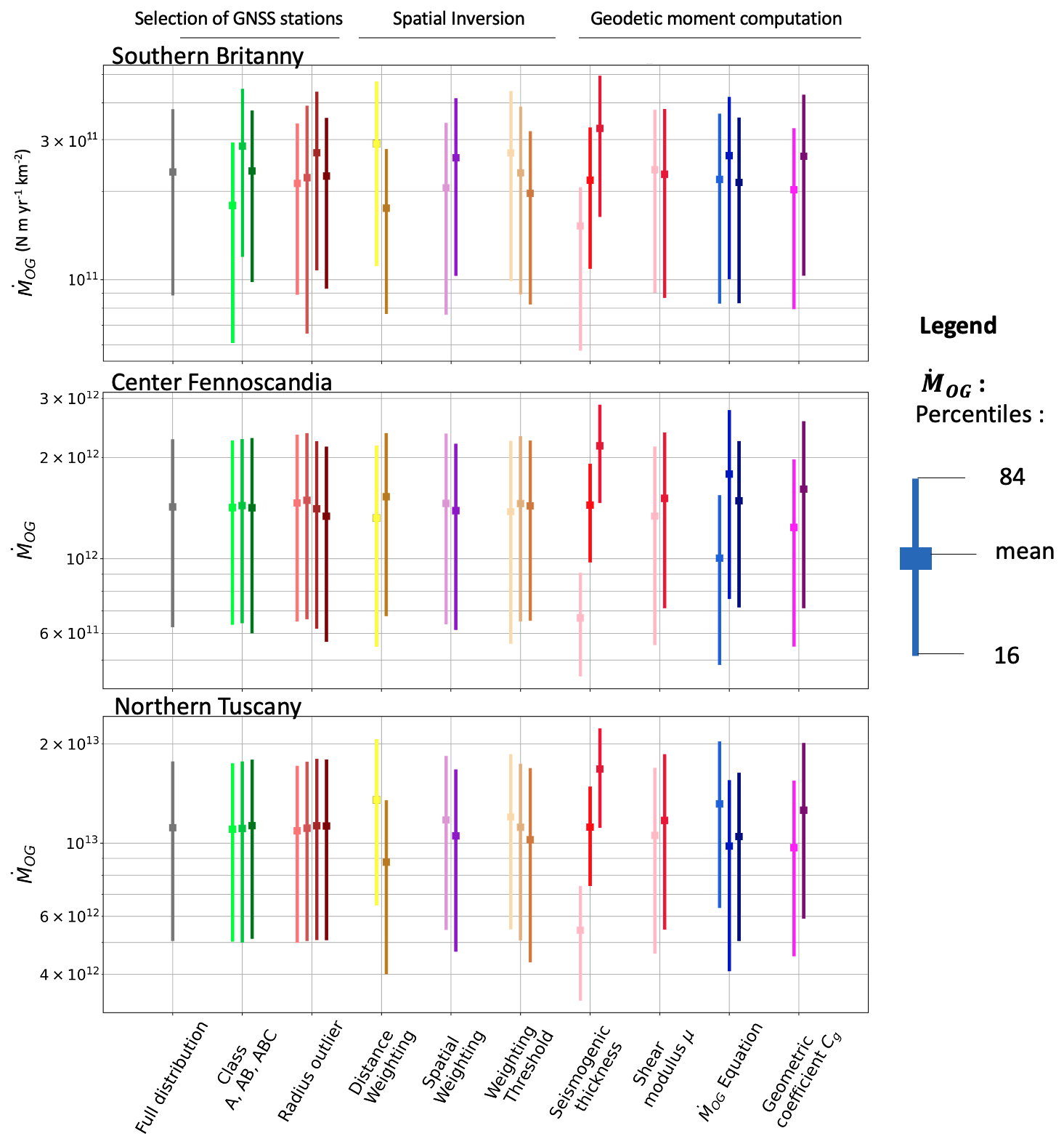
Figure 5 Distribution for the geodetic moment rate (${\dot{M}}_{\mathrm{0}\mathrm{G}}$) and identification of controlling parameters, in three example source zones: southern Brittany (FRAS176), Fennoscandia (SEAS410), and northern Tuscany in Italy (ITAS335); see location in Fig. 6. Mean value (square) and 16th and 84th percentiles (vertical bar). “Full distribution” – full exploration of the tree (5184 branches' combination and moment values). “Class A, AB, ABC” – three different sets of GNSS stations, according to quality (1728 values each). “Radius outlier” – choice of the spatial radius for discarding outliers (50, 100, 150, 200 km; from salmon to dark red, 1296 values each). “Distance weighting scheme” – choice of the decay function used for interpolation, whether Gaussian or quadratic (2592 values each). “Spatial weighting scheme” – choice of the method for spatial inversion, whether azimuth or Voronoi. “Weighting threshold” – choice of the threshold value on the distance weighting function (6, 12, 24; increasing smoothing; beige to brown; 1728 values each). “Seismogenic thickness” – elastic thickness (5, 10, and 15 km; pink to red; 1728 values each). “μ” – choice of shear modulus value (3.3×10¹⁰ N m (pink), 3×10¹⁰ N m (red)). “${\dot{M}}_{\mathrm{0}\mathrm{G}}$ equation” – choice of the geodetic moment equation; see the text. “C_g” – choice of the geometric coefficient parameter, 2 (light purple) or 2.6 (dark purple).

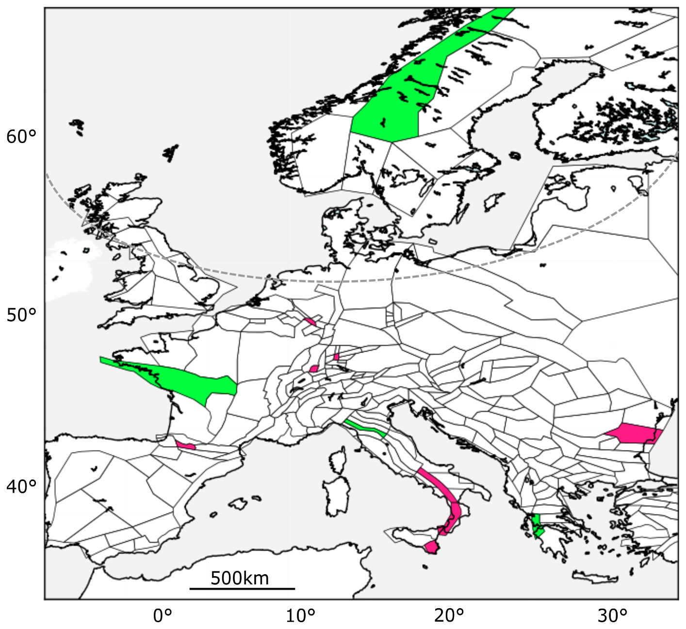
Figure 6 Area source zones mentioned throughout the paper. In pink: the eight source zones where the geodetic moment estimates are much lower than the seismic moment estimates (Sect. 3.1.3 and Fig. 10). 1 – ITAS308, 2 – ITAS331, 3 – ITAS339, 4 – BGAS043, 5 – FRAS164, 6 – DEAS113, 7 – DEAS109, 8 – CHAS071. The dashed gray line represents the zones considered affected by the Scandinavian glacial isostatic adjustment (GIA), including those intersecting this line and those located to the north of the line. The selection is based on the vertical velocity signal (Piña-Valdés et al., 2022) and includes 18 zones. In green: example source zones in Sect. 2.2.3. 9 – FRAS176 in southern Brittany in France, 10 – SEAS410 in Fennoscandia, 11 – ITAS335 in northern Italy, and 12 – GRAS257 in Greece in Sect. 3.1.2.

The results show that all parameters but the shear modulus contribute to the overall uncertainty in the geodetic moment rate. The parameter that contributes the most is the effective seismogenic thickness. The geodetic moment rate is linearly correlated with both the effective seismic thickness and the shear modulus. We accounted for only a small uncertainty in the shear modulus (10 % variability). It is interesting to note that the exact selection of GNSS stations, controlled by the selection steps related to the class and the radius outlier, has an influence on the moment rate estimates in low-seismicity regions (Fennoscandia and southern Brittany) but no impact in the moderate- to high-seismicity regions (such as northern Tuscany). This phenomenon can be attributed to the high strains in high-deformation zones, where even lower-quality stations provide accurate measurements at a first-order approximation. Conversely, in low-deformation areas, the measured signal is close to the noise level (hence, highly uncertain), and the exclusion or inclusion of one or more stations has a strong impact. Furthermore, it is noteworthy that the parameters involved in the spatial inversion, particularly the distance weighting scheme, have a significant impact on the overall uncertainty. This impact is more pronounced in regions with a relatively high density of GNSS stations, such as northern Tuscany and southern Brittany. The Gaussian function reduces data weight with distance faster than the quadratic function, which can yield a smoother solution when dealing with heterogeneous data. In regions with a high density of stations, this may lead to higher strain rates calculated using the Gaussian function than those obtained with the quadratic function. Additionally, the weighting threshold, which controls the smoothing of the solution, naturally has a greater impact in regions with a higher station density. The results also highlight that the equation used to convert surface strain into scalar moment rate can have a significant impact (in blue in Fig. 5). The uncertainty in the choice of the equation contributes to the overall variability of the moment rate.

3 Results

3.1 Is the ESHM20 earthquake rate forecast consistent with the tectonic loading measured by geodesy?

Our aim is to compare the moment rate corresponding to the long-term ESHM20 earthquake rate forecast with the geodetic moment rate. We acknowledge that the comparison between deformation measurements performed over a few decades and a seismogenic source model for a regional seismic hazard assessment must be done with caution. The ESHM20 earthquake rate forecast relies on earthquake catalogs extending over several centuries in most regions of the study area. The recurrence model is in general anchored on the observed earthquake rates extrapolated up to magnitudes that correspond to the largest possible events in the area sources. The model thus relies on both recent observations (instrumental earthquake catalogue) and past historical seismicity as well as on a wider analysis of the seismogenic potential of the area. The earthquake rate forecast model also includes our current knowledge about active faults (fault traces, segmentation, extension at depth; see Basili et al., 2024). Geodetic information has been used in some cases for estimating the deformation accumulating along these faults (Basili et al., 2024). The strain model is thus not strictly independent of the source model; however GNSS velocities have not been directly used to build the ESHM20 source model. The strain rate model can be used to test the ESHM20 source model and evaluate how realistic it is.

3.1.1 Correlation between geodetic and seismic moment rates at the scale of Europe

The geodetic moment rate quantifies the ground surface deformation that encompasses both seismic and aseismic processes. The mean moment estimates obtained in every area source zone are displayed in Fig. 7. Overall, geodetic moment rates appear to be larger than or equal to seismic moment rates, similar to the findings of many previous studies (e.g., Ward, 1998; Jenny et al., 2004; Mazzotti et al., 2011). The largest geodetic and seismic rates are found in Greece, Italy, and the Balkans. The distribution in space of the geodetic moment rate is much more smoothed than that of the seismic moment rate. One explanation could be that the deformation measured by geodesy is more representative of long-term processes than the earthquake catalogs. If earthquake catalogs of much longer time windows were available (e.g., 100 000 years), would the spatial distribution of the seismic moment rates be more similar to the spatial distribution of the geodetic moment rates? We do not know. Another explanation could be that the geodetic moment rate has a lower resolution in space than the seismic moment rate inferred from the modeling of earthquake recurrence. Due to the smoothing procedure applied to derive the strain rates, the geodetic moment is strongly correlated spatially.

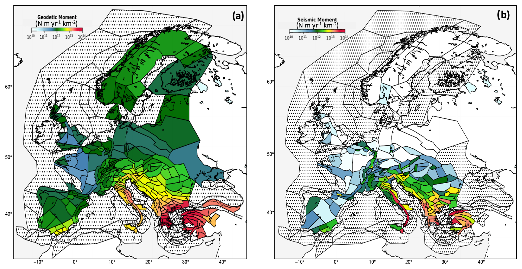
Figure 7 Mean geodetic and seismic moment rates within the ESHM20 area source zones. (a) Mean geodetic moment (${\dot{M}}_{\mathrm{0}\mathrm{G}}$) based on the strain rates and mean of the distribution obtained by exploring uncertainties. (b) Mean seismic moment (${\dot{M}}_{\mathrm{0}\mathrm{S}}$) estimated from the ESHM20 source model logic tree. Area sources with more than 35 % of surface offshore or where the density of GNSS stations is too low (≤ one station per 100 000 km²) are discarded. Area source zone polygons can also be found in Fig. 6.

Figure 8 shows a comparison between geodetic and seismic mean moments in Europe at the scale of the ESHM20 area source zones. It demonstrates a remarkable linear correlation between the geodetic and seismic moment rates above ∼ 2×10¹¹ N m yr⁻¹ km⁻². In general, in the most active regions in southern Europe, the geodetic moment rates are well-correlated with the seismic moment rates. On the contrary, in the less active regions in northern Europe, above ∼ 50° latitude, the geodetic moment appears completely decorrelated from the seismic moment. Seismic moment rates decrease to levels as low as 10⁹–10¹⁰ N m yr⁻¹ km⁻², whereas geodetic moment rates reach a plateau around 10¹² N m yr⁻¹ km⁻². The deformation measured in Fennoscandia and surrounding regions might be mostly related to the post-glacial rebound, and only a very small part of it might be tectonic deformation (Keiding et al., 2015; Craig et al., 2016).

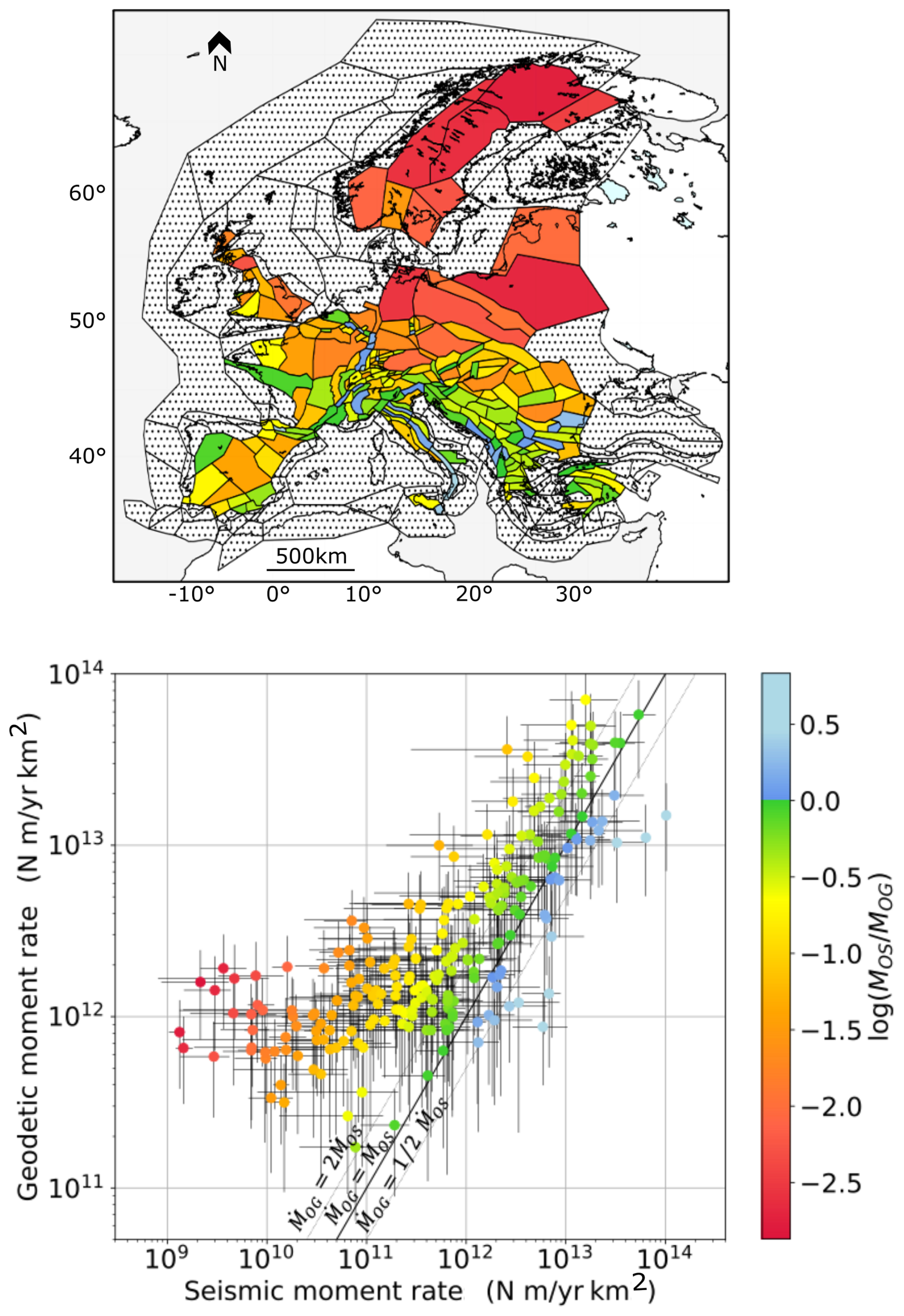
Figure 8 Comparison between geodetic and seismic moment rates in Europe at the scale of the ESHM20 source zones: mean ${\dot{M}}_{\mathrm{0}\mathrm{G}}$ versus mean ${\dot{M}}_{\mathrm{0}\mathrm{S}}$ at the scale of the source zone (uncertainty range in the 16th to 84th percentiles indicated). Area source zone polygons can also be found in Fig. 6.

3.1.2 Comparison of the moment rate distributions

Rather than comparing only mean values of distributions, the comparison of the full distributions can be more instructive as the uncertainties are accounted for. For a given area source zone, the distribution for the geodetic moment rate relies on 5184 alternative values (see Sect. 2.2.3). The distribution for the seismic moment is built by exploring the ESHM20 source model logic tree, taking into account the weights associated with each branch.

In Fennoscandia, the geodetic moment estimates are on average 100 to 300 times higher than the seismic moment estimates $\left({\log }_{\mathrm{10}}\right({\dot{M}}_{\mathrm{0}\mathrm{S}}/{\dot{M}}_{\mathrm{0}\mathrm{G}})$ varies between −2 and −2.5, in red in Fig. 8). The uncertainty in the geodetic moment is large, but still there is no overlap between the two distributions (example source zone SEAS410, Fig. 9). In most area sources below 52° latitude, geodetic moment estimates are larger than or equal to seismic moment rates, being up to 5 times higher on average than seismic moment rates $\left({\log }_{\mathrm{10}}\right({\dot{M}}_{\mathrm{0}\mathrm{S}}/{\dot{M}}_{\mathrm{0}\mathrm{G}})$ varies between 0 and −0.7, in green and yellow in Fig. 8). In some area sources such as GRAS257 in Greece, the mean geodetic moment rate is 5 times higher than the mean seismic moment rate, and their distributions only partially overlap. In other source zones, such as FRAS176 in France or ITAS335 in Italy, the seismic and geodetic distributions are very consistent.

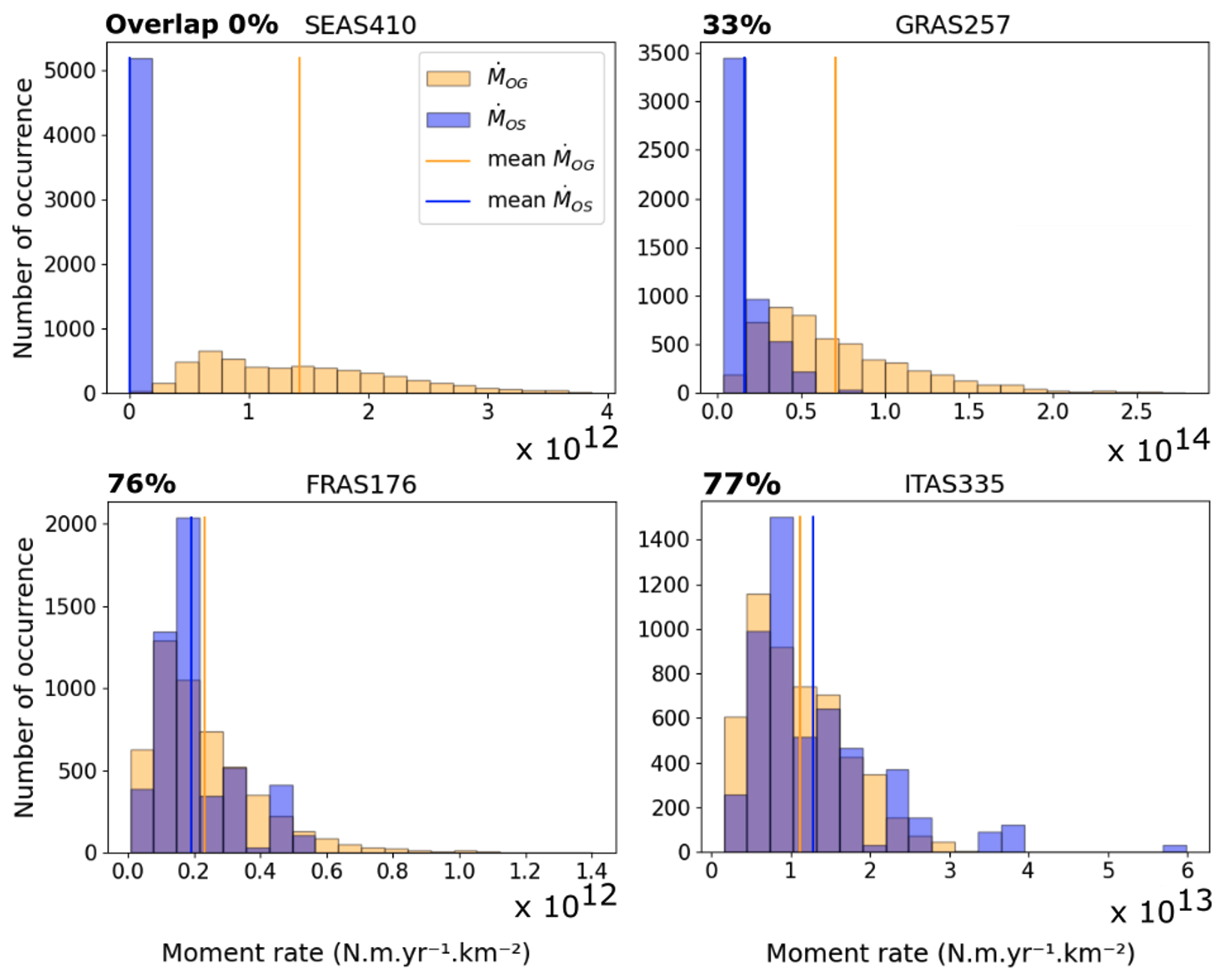
Figure 9 Comparison of seismic and geodetic moment rate distributions for four example source zones in Fennoscandia (SEAS410), Greece (GRAS257), France (FRAS176), and Italy (ITAS335), with source zones in Fig. 6. The percentage of overlap of both distributions is indicated in the title.

We quantify the overlap between the geodetic and the seismic distributions for all area sources (Fig. 10). As the distributions are in most cases unimodal, the overlap between the distributions usually improves with closer mean moment values. In the most seismically active regions in Europe, i.e., in Greece, Italy, and the Balkans, as well as in some parts of France and Switzerland, the seismic and geodetic moment estimates are rather consistent (overlap between 35 % and 80 %, in blue), whereas in most of northern Europe, the fit is quite poor (overlap lower than 30 %, in red).

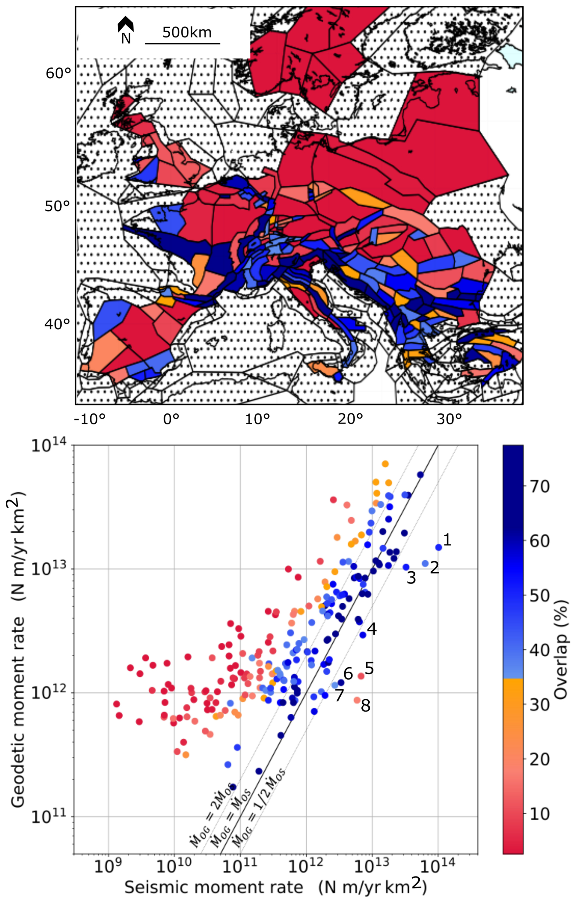
Figure 10 Comparison between geodetic and seismic moment rate mean estimates, within the ESHM20 shallow area source zones (227 source zones considered), and estimates for the overlap between the seismic and geodetic distributions. Shallow area source zones where the geodetic moment rate is much lower than the seismic moment rate: 1 – ITAS308, 2 – ITAS331, 3 – ITAS339, 4 – BGAS043, 5 – FRAS164, 6 – DEAS113, 7 – DEAS109, and 8 – CHAS071 (see the text and Fig. 6).

As the size of some source zones is too small for the comparison to be meaningful (see Sect. 3.1.3), we also perform the comparison at the macrozone scale. Macrozones include several area source zones. They are used at different levels in the building of the ESHM20 source model, e.g., to determine spatial variations in the completeness time windows of the earthquake catalog or to define tectonic similarities and maximum magnitude throughout Europe (Danciu et al., 2024; Basili et al., 2024). Here we use the macrozones named “TECTO”, which correspond to a seismotectonic regionalization (Fig. 2). Danciu et al. (2021a, 2024) used these macrozones to evaluate the b value for the smoothed seismicity model for the underlying crustal active faults and to constrain recurrence parameters of area sources without a sufficient number of earthquakes. As expected, at the scale of Europe, the correlation between the seismic and geodetic moment rates is slightly improved when considering the macrozones, which cover a much larger spatial region than the individual area source zones (see Fig. 2). In regions of northern Europe, the overlap between geodetic and seismic moment distributions is low (below 35 %, in red). A rather good fit is obtained for the Euro-Mediterranean region (overlap above 35 %, in blue), except in Spain (Fig. 11). A more detailed analysis focusing on Spain would be necessary to understand why.

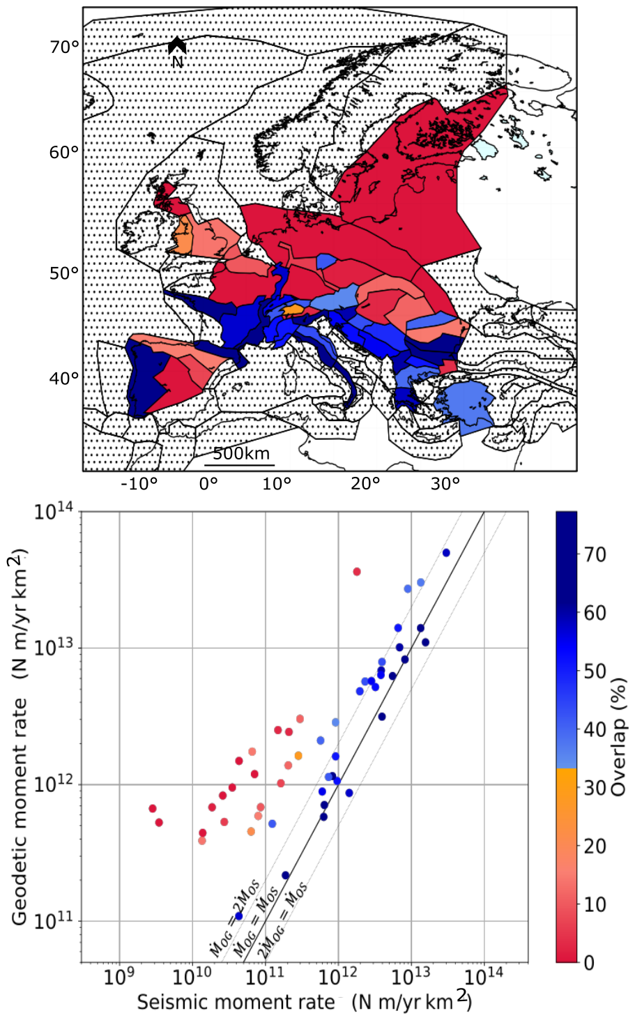
Figure 11 Comparison between geodetic and seismic moment rate mean estimates within the ESHM20 TECTO macrozones (51 macrozones considered). The amount of overlap between the seismic and geodetic distributions is indicated.

3.1.3 A closer look into the area sources with a seismic moment much higher than the geodetic moment

In eight area source zones, the geodetic moment rate is, on average, significantly lower than the seismic moment rate (data points that are below the straight line ${\dot{M}}_{\mathrm{0}\mathrm{G}}$ = ${\dot{M}}_{\mathrm{0}\mathrm{S}}/\mathrm{2}$ in Fig. 8).

These area sources fall into three categories:

1. The first category is small-size areas, below the resolution of the geodetic signal (FRAS164, CHAS071, DEAS113, DEAS109). The source zone FRAS164 in the western Pyrenees is a small area with very high seismic activity in comparison with the neighboring area zones. The geodetic signal has a spatial wavelength that is too large to capture these rapid spatial changes. The source zones CHAS071 (Switzerland), DEAS113 (Germany), and DEAS109 (Germany) are not as active as FRAS164, but they are very small size area sources. In these cases, the difference between the geodetic and the seismic moment estimates is expected.

2. The second category is areas with a poorly constrained earthquake recurrence model due to an insufficient number of events for statistical fitting (i.e., ITAS339 or BGAS043). In those areas, the resulting ESHM20 recurrence model fits the observed rates in the upper-magnitude range but predicts larger seismic rates than what has been observed in the past in the moderate-magnitude range. There are too few data to constrain the model. The b value is inferred from the larger macrozone, whereas the seismic activity is estimated by re-scaling the occurrence rates as a function of the number of complete earthquakes (the scaling factor is the ratio between the number of complete events in the area source and the number of complete events in the corresponding macrozone, Danciu et al., 2021a).

3. The third category is areas where unusual earthquake recurrence models have been proposed to account for two different slopes observed in the Gutenberg–Richter model (area model, ITAS331, ITAS308). In both area sources, the slope of the recurrence model in the upper-magnitude range (mostly historical period) is lower than the slope in the moderate-magnitude range (mostly instrumental period). This is not due to a lack of data. A double-slope Gutenberg–Richter distribution has been used. It is interesting to note that the fault model branches overall provide a moment range that is consistent with the geodetic moment range, whereas the area model branches lead to much higher moment estimates.

3.1.4 The consistency between the geodetic and seismic moments depends on the activity level, the spatial scale, and the source model

Figure 12 provides an overall view on the comparison between geodetic and seismic moment estimates at the scale of Europe and how this comparison varies when subsets of areas or branches of the ESHM20 source model logic tree are selected. Distributions for the ratio ${\log }_{\mathrm{10}}({\dot{M}}_{\mathrm{0}\mathrm{S}}/{\dot{M}}_{\mathrm{0}\mathrm{G}})$ are characterized by mean values, as well as 16th and 84th percentiles (boxplots). When ${\log }_{\mathrm{10}}({\dot{M}}_{\mathrm{0}\mathrm{S}}/{\dot{M}}_{\mathrm{0}\mathrm{G}})$ tends towards 0, ${\dot{M}}_{\mathrm{0}\mathrm{S}}$ and ${\dot{M}}_{\mathrm{0}\mathrm{G}}$ get closer. Area source zones are also grouped according to their level of geodetic moment estimates (dark green, light green, red), showing that, when all area source zones are considered, the consistency improves with increasing deformation rate.

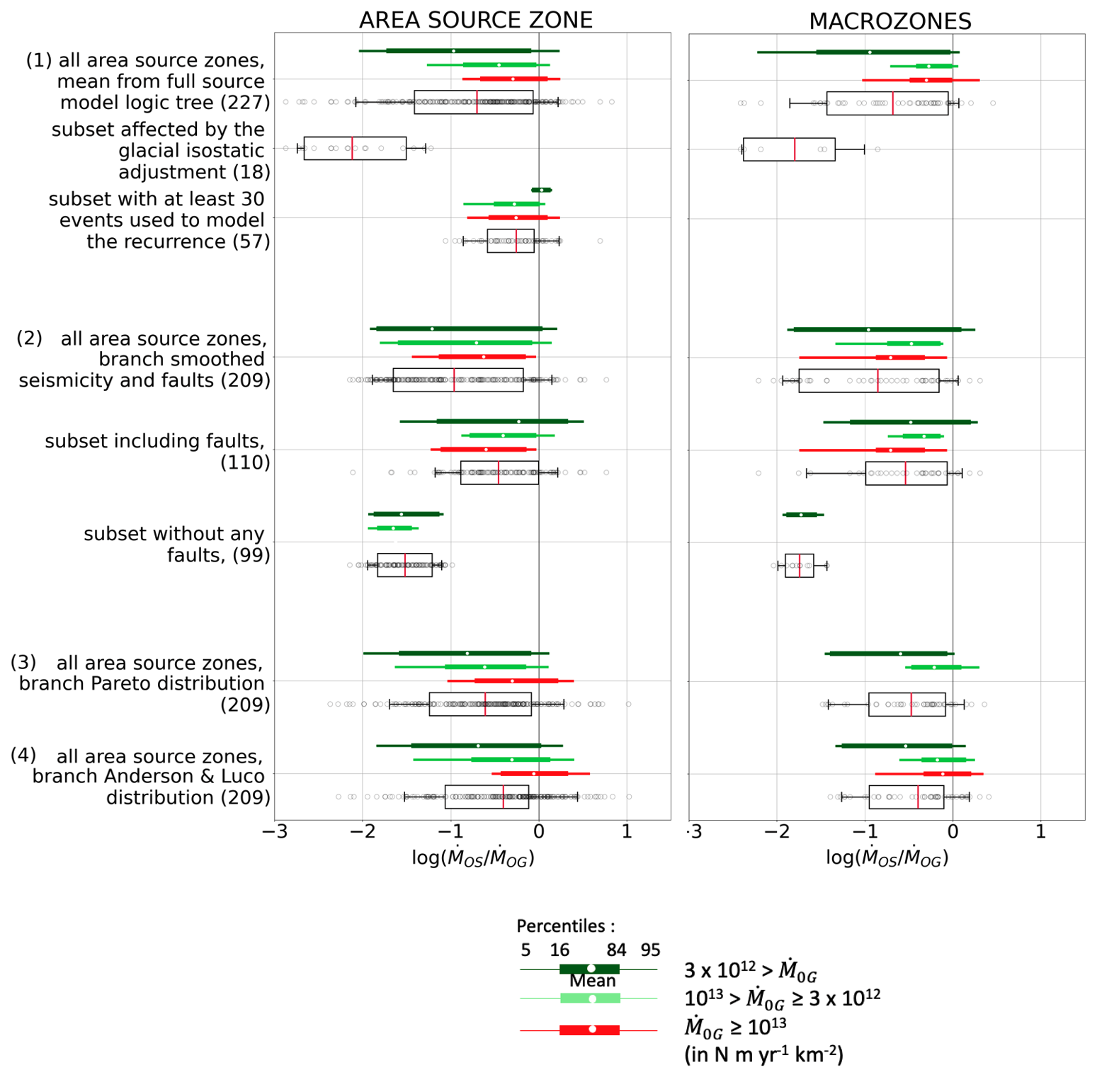
Figure 12 Consistency between ${\dot{M}}_{\mathrm{0}\mathrm{S}}$ and ${\dot{M}}_{\mathrm{0}\mathrm{G}}$ at the area source zone scale (left) and at the macrozone scale (right). Whisker plots indicate the mean, as well as the 16th and 84th and 5th and 95th percentiles. Black circles – individual ratio per source zone. Area sources are also grouped per increasing geodetic moment level: dark green ${\dot{M}}_{\mathrm{0}\mathrm{G}}>\mathrm{3}\times {\mathrm{10}}^{\mathrm{12}}$ N m yr⁻¹ km⁻², green $\mathrm{3}\times {\mathrm{10}}^{\mathrm{12}}<{\dot{M}}_{\mathrm{0}\mathrm{G}}<{\mathrm{10}}^{\mathrm{13}}$ N m yr⁻¹ km⁻², and red ${\dot{M}}_{\mathrm{0}\mathrm{G}}>{\mathrm{10}}^{\mathrm{13}}$ Nm yr⁻¹ km⁻². In subsets (2), (3), and (4), the 18 zones affected by the Fennoscandian glacial isostatic adjustment (GIA) have been discarded (see Fig. 6). A total of 227 area source zones are considered, including 18 affected by GIA, 57 well-constrained recurrence models, and 110 that include faults.

In area source zones affected by the glacial isostatic adjustment (18 zones, selected based on their vertical velocity signal, Piña-Valdés et al., 2022), both the geodetic and the seismic moments are low, but the moment estimate based on modeled earthquake recurrence distributions is 2 orders of magnitude lower than the geodetic moment. This suggests that the deformation processes involved are mostly aseismic, which is compatible with the processes involved in glacial isostatic adjustment (GIA). GIA generates a viscous asthenospheric flow and a large-scale flexure of the overlying elastic lithosphere that results in rather large wavelength deformation (i.e., the strain is distributed over a large area, Mazzotti et al., 2011; Piña-Valdés et al., 2022). It should also be noted that the post-glacial rebound is a phenomenon that is not representative of the long-term (a few million years) tectonics but that it is a transient mechanism that started after the last glacial maximum, ≈ 20 000 years ago (Steffen and Wu, 2011). The cumulative deformation associated with the glacial isostatic adjustment may therefore not reach locally the strength threshold of the Fennoscandian lithosphere, although this may vary spatially depending on the elastic thickness of the crust (Pérez‐Gussinyé et al., 2004). In those areas, the surface deformation measured by geodesy is therefore not a suitable proxy for the seismic activity and can not be used directly to constrain earthquake recurrence models.

Considering area sources with the best-constrained recurrence models (at least 30 events used to estimate recurrence parameters; see Danciu et al., 2021a), the consistency between both moment rate estimates is strongly improved. In general, the zones with the largest number of events falling inside periods of completeness are the zones with the highest seismic activity.

The compatibility between geodetic and seismic moment rates varies depending on the branch of the ESHM20 seismogenic source model logic tree, (2), (3), and (4) in Fig. 12, from which the zones affected by GIA have been removed. Considering the smoothed seismicity and fault model branch, the seismic moment rates are overall less consistent with the geodetic moment rates than in the area model. The comparison is done at the scale of the area sources. We group the area zones that include faults on one side and the area zones that do not include any faults on the other side (see Fig. 1). We observe that the geodetic and seismic moment rates are much more consistent in the first group, where the faults have mostly been characterized in the most seismically active parts of Europe. Considering the area branch of ESHM20 models (3) and (4) in Fig. 12, we check if the fit between geodetic and seismic moment rates varies with the model selected to extrapolate earthquake rates in the upper-magnitude range. The fit is slightly better using the classical Anderson and Luco (1983) form (2) compared to the Pareto distribution. This result is expected, as the Pareto distribution implies a stronger decrease in seismic rates in the upper-magnitude range with respect to the Anderson and Luco distribution (therefore a lower seismic moment rate). We also perform the comparison at the scale of the macrozones (right column). The correlation between the seismic and geodetic moment rates is slightly improved, mean values of distributions tend to be closer to 0, and macrozones cover a much larger spatial region than the individual area source zones.

The improved consistency between seismic and geodetic moments with increasing deformation rates is also observable in Fig. 13, which displays the ratio ${\log }_{\mathrm{10}}({\dot{M}}_{\mathrm{0}\mathrm{S}}/{\dot{M}}_{\mathrm{0}\mathrm{G}})$ as a function of the number of earthquakes used to constrain the earthquake recurrence model in the corresponding area source. The size of the symbol increases with the density of faults in the zone, and the color reflects the level of the geodetic moment (as in Fig. 12). This figure shows mean values only. Zones with the highest geodetic moment rates exhibit better consistency between ${\dot{M}}_{\mathrm{0}\mathrm{S}}$ and ${\dot{M}}_{\mathrm{0}\mathrm{G}}$ (all zones with ${\dot{M}}_{\mathrm{0}\mathrm{G}}$ ≥ 10¹³ N m yr⁻¹ km⁻², in red, fall within the ${\log }_{\mathrm{10}}({\dot{M}}_{\mathrm{0}\mathrm{S}}/{\dot{M}}_{\mathrm{0}\mathrm{G}})$ interval of −1 to 0.5). Zones with ${\log }_{\mathrm{10}}({\dot{M}}_{\mathrm{0}\mathrm{S}}/{\dot{M}}_{\mathrm{0}\mathrm{G}})$ below −1 are mostly characterized by low strain rates (${\dot{M}}_{\mathrm{0}\mathrm{G}}$ ≤ 3×10¹² N m yr⁻¹ km⁻²) and include areas affected by GIA. In areas where the recurrence model was constrained with at least 50 events (most active areas in Europe), the ${\log }_{\mathrm{10}}({\dot{M}}_{\mathrm{0}\mathrm{S}}/{\dot{M}}_{\mathrm{0}\mathrm{G}})$ ratios fall mostly between −0.5 and 0.5 (i.e., the ratios between seismic and geodetic moment rates are within a factor of $\mathrm{1}/\mathrm{3}$ to 3).

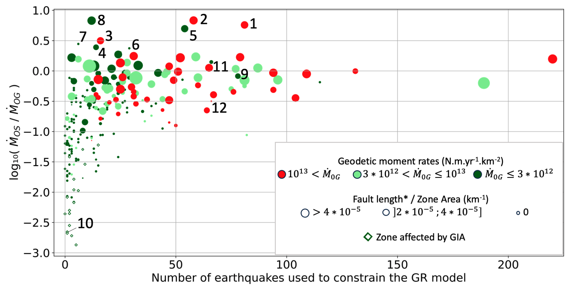
Figure 13 Mean ${\log }_{\mathrm{10}}({\dot{M}}_{\mathrm{0}\mathrm{S}}/{\dot{M}}_{\mathrm{0}\mathrm{G}})$ for all source zones in Europe, as a function of the number of earthquakes used to constrain the earthquake recurrence model (M_W ≥ 3.5). The color represents the mean geodetic moment of the source zone area, and the size of the symbol is proportional to the density of the faults that have been included in the model, with slip rates higher than 0.1 mm yr⁻¹ (^*) in the ESHM20 fault model. Compatibility between geodetic and seismic moment rates increases with the geodetic moment rates, the number of earthquakes used to constrain the earthquake recurrence model, and the fault density. Area source zones where the geodetic moment rate is much lower than the seismic moment rate: 1 – ITAS308, 2 – ITAS331, 3 – ITAS339, 4 – BGAS043, 5 – FRAS164, 6 – DEAS113, 7 – DEAS109, and 8 – CHAS071. Example source zones in Sect. 2.2.3: 9 – FRAS176, 10 – SEAS410, 11 – ITAS335, and 12 – GRAS257 (see the text and Fig. 6).

Figure 13 also highlights the impact of active fault density on the consistency between geodetic moment rates. The active fault density for each zone is defined as the length of faults with a slip rate exceeding 0.1 mm yr⁻¹, divided by the zone's area (expressed in km⁻¹). Zones with a density above $\mathrm{4}\times {\mathrm{10}}^{-\mathrm{5}}$ km⁻¹ display a ${\log }_{\mathrm{10}}({\dot{M}}_{\mathrm{0}\mathrm{S}}/{\dot{M}}_{\mathrm{0}\mathrm{G}})$ between −1 and 1, with the majority falling within −0.5 and 0.5. In regions with higher active fault density, the compatibility between ${\dot{M}}_{\mathrm{0}\mathrm{S}}$ and ${\dot{M}}_{\mathrm{0}\mathrm{G}}$ is improved. Regions where a fault model can be included for seismic hazard assessment are in general seismically active regions. Similar results are observed in Fig. 12 (part 2) when we consider only the ESHM20 model branch based on smoothed seismicity and faults (although this branch exhibits seismic and geodetic moment rate estimates that are overall less consistent than those of the other branches of ESHM20). We observe that the geodetic and seismic moment rates are much better correlated in the area zones that include faults than in area zones that do not include any faults in the model. This is correlated to the activity of the area, since the faults are easier to map and characterize in the seismically active region. However, in Figs. 12 (2) and 13, we can observe that in zones with lower strain (${\dot{M}}_{\mathrm{0}\mathrm{G}}$ ≤ 3×10¹² N m yr⁻¹ km⁻²), when either the fault density or the number of earthquakes used to constrain the earthquake recurrence model increases, ${\log }_{\mathrm{10}}({\dot{M}}_{\mathrm{0}\mathrm{S}}/{\dot{M}}_{\mathrm{0}\mathrm{G}})$ gets closer to 0. Zones with ${\log }_{\mathrm{10}}({\dot{M}}_{\mathrm{0}\mathrm{S}}/{\dot{M}}_{\mathrm{0}\mathrm{G}})$ below −1 are all characterized by a minimum fault density (≤ $\mathrm{2}\times {\mathrm{10}}^{-\mathrm{5}}$ km⁻¹) and less than 30 earthquakes used to constrain the earthquake recurrence model. This corroborates the idea that the inclusion of active faults may strengthen the earthquake recurrence model in areas that are characterized by both a slow deformation rate and rare seismic events. As a corollary, this may indicate that, in areas where enough active faults are identified and mapped, the geodetic moment rate may be used as a proxy for the long-term tectonic loading, even in areas where a limited number of earthquakes is available to constrain the recurrence model.

4 Discussion

4.1 Focus in Italy

Figure 14a presents a magnified view of Fig. 8a in central Italy. As highlighted previously, the central zone (ITAS317) demonstrates a mean seismic moment (${\dot{M}}_{\mathrm{0}\mathrm{S}}$) exceeding the mean geodetic moment $\left({\dot{M}}_{\mathrm{0}\mathrm{G}}\right)$ $\left({\log }_{\mathrm{10}}\right({\dot{M}}_{\mathrm{0}\mathrm{S}}/{\dot{M}}_{\mathrm{0}\mathrm{G}})>\mathrm{0})$. Conversely, the surrounding zones exhibit a geodetic moment that is significantly higher than the seismic moment $\left({\log }_{\mathrm{10}}\right({\dot{M}}_{\mathrm{0}\mathrm{S}}/{\dot{M}}_{\mathrm{0}\mathrm{G}})$ ∼ −1, overlap < 20 %). Performing the comparison at the scale of the macrozones, this discrepancy is reduced because of the spatial smoothing of the signal (Fig. 11). In this section, we analyze the reasons for such a peak of seismic release by examining the seismic moment against the geodetic moment along a profile across the Apennines passing through Rome (profile AB in Fig. 14a and b).

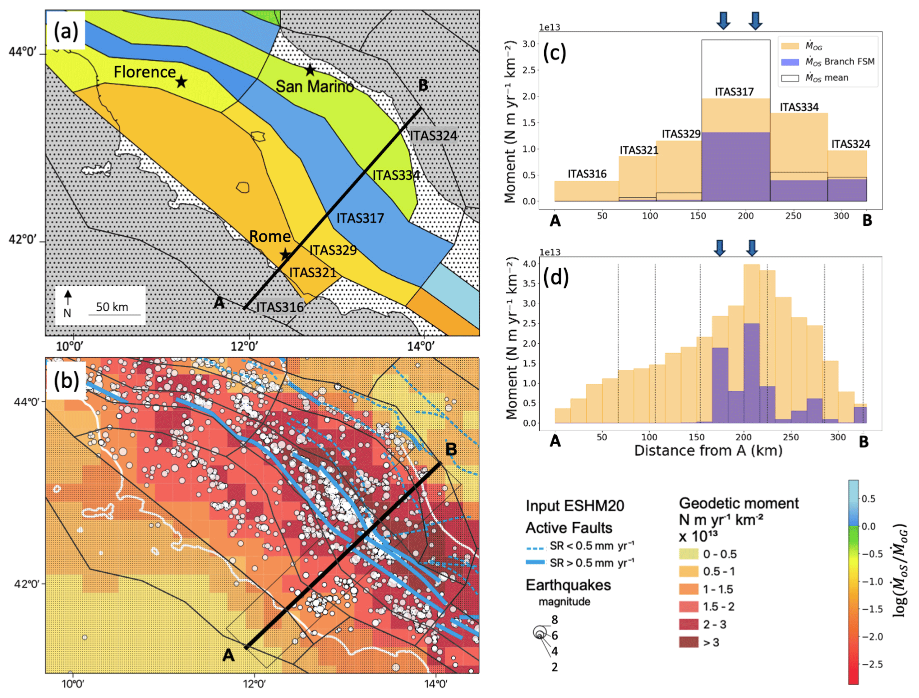
Figure 14 Spatial variability of geodetic deformation and seismic release in the central Apennines. (a) Zoomed-in view of Fig. 8a – mean ratio between ${\dot{M}}_{\mathrm{0}\mathrm{S}}$ and ${\dot{M}}_{\mathrm{0}\mathrm{G}}$ for area source zones in central Italy. (b) Mean geodetic moment rate per surface unit inferred from strain rates; gray dots – earthquakes in the ESHM20 unified earthquake catalog, blue lines – active faults included in the EFSM20. (c, d) Geodetic (${\dot{M}}_{\mathrm{0}\mathrm{G}}$) and seismic (${\dot{M}}_{\mathrm{0}\mathrm{S}}$) moment rates per kilometer along the cross-section AB, averaged within the source zones (c) or averaged within bins of 14 km along a 190 km wide swath profile, represented by the thin gray rectangle. (d) Blue arrows – location of the two main faults.

Figure 14a presents the ratio between the estimated ${\dot{M}}_{\mathrm{0}\mathrm{S}}$ and ${\dot{M}}_{\mathrm{0}\mathrm{G}}$ at the scale of the source zones. Figure 14c provides a view of how these moments are distributed as a function of the distance along the cross-section AB: the average geodetic (${\dot{M}}_{\mathrm{0}\mathrm{G}}$) and seismic (${\dot{M}}_{\mathrm{0}\mathrm{S}}$) moment rates are represented by plain orange bars and empty black bars, respectively. ${\dot{M}}_{\mathrm{0}\mathrm{G}}$ exceeds the mean ${\dot{M}}_{\mathrm{0}\mathrm{S}}$ in all source zones (5 to 10 times larger), except in the central source zone (ITAS317), which is the most seismically active and encompasses several faults. In this particular source zone, ${\dot{M}}_{\mathrm{0}\mathrm{S}}$ exceeds ${\dot{M}}_{\mathrm{0}\mathrm{G}}$.

Then, we use the fault and smoothed seismicity model of ESHM20 to compare the seismic moments with the geodetic moments evaluated on the same spatial grid. It should however be noted that the fault and smoothed seismicity model (purple bars) exhibits seismic moments that are systematically lower than the mean inferred from the full ESHM20 source model logic tree (Figs. 12, 14). ${\dot{M}}_{\mathrm{0}\mathrm{S}}$ and ${\dot{M}}_{\mathrm{0}\mathrm{G}}$ are compared along a profile AB, averaged within spatial bins of 14 km (Fig. 14d). This analysis at a finer scale reveals that ${\dot{M}}_{\mathrm{0}\mathrm{S}}$ is concentrated on the fault traces, marked with small blue arrows. ${\dot{M}}_{\mathrm{0}\mathrm{G}}$ exhibits a smoother behavior and reaches its maximum (4×10¹³ N m yr⁻¹ km⁻²) at the level of the eastern fault (similar to ${\dot{M}}_{\mathrm{0}\mathrm{S}}$).

Several propositions can be put forth to explain this observation. Firstly, we may question whether the spatial regularization scheme used during the strain map inversion could lead to a smoothing of the solution. In Italy the density of GPS stations is quite high, with an interstation distance of 20 km on average, and the network should capture any spatial details larger than 30 km in the deformation field (Piña-Valdés et al., 2022). The observed difference in spatial distribution between the seismic moment release and the geodetic moment is most likely real.

Another possible explanation is to invoke the elastic rebound theory. In areas affected by major active faults, the faults accumulate elastic strain that is then released into earthquakes. During the interseismic period, the deformation associated with the loading is usually modeled as a fault that is locked down to a given depth and that creeps at the loading rate at greater depths (Avouac, 2015). This generates a surface deformation that has a large spatial wavelength. The deeper the locking, the wider the deformation across the fault. In elastic rebound theory (Reid, 1910), the slip deficit accumulated during the loading phase is then released into earthquakes located on the fault plane. The elastic rebound theory can therefore explain the observed differences in the spatial distribution of ${\dot{M}}_{\mathrm{0}\mathrm{S}}$ and ${\dot{M}}_{\mathrm{0}\mathrm{G}}$ across the Apennines. In areas where the deformation mechanism is dominated by the seismic cycle on active faults, a proper modeling of the interseismic coupling on the faults would be better adapted (Mariniere, 2020; Mariniere et al., 2021).

We can conclude that the scale at which deformation is observed is a crucial criterion for analyzing the compatibility between seismic and geodetic moments. Therefore, in places where source zones enclose active faults or areas with high seismic activity, the comparison between the geodetic moment and the seismic moment can be meaningful only if it is led at a large enough spatial scale.

4.2 Focus in France

We focus on the area source zones included in metropolitan France or located on the border with neighboring countries (Fig. 15). The distributions of the geodetic and seismic moments determined for each zone are compared in Fig. 16, with source zones ordered according to increasing number of earthquakes used to constrain the recurrence models in ESHM20. In regions of very low seismicity, with magnitude–frequency distributions relying on less than 10 events within completeness periods, the distribution of the seismic moment (${\dot{M}}_{\mathrm{0}\mathrm{S}}$) is systematically much lower than the distribution of the geodetic moment (${\dot{M}}_{\mathrm{0}\mathrm{G}}$), with no overlap. In area sources with more than 18 events used to establish the recurrence model, both distributions tend to overlap. There are exceptions, such as FRAS164 in the western Pyrenees, a small zone with high seismic activity with respect to the rest of the Pyrenees (as explained in Sect. 3.1.3). France includes source zones where the fit between the distributions is rather good (in blue), similar to the Euro-Mediterranean regions, as well as source zones where the geodetic moment rates are much higher than the seismic moment rates, similar to the Fennoscandia region.

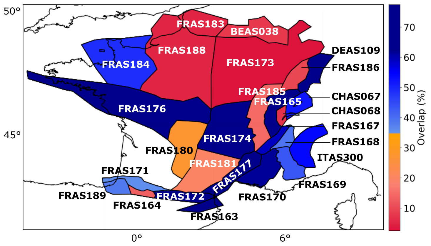
Figure 15 Consistency between ${\dot{M}}_{\mathrm{0}\mathrm{G}}$ and ${\dot{M}}_{\mathrm{0}\mathrm{S}}$ distributions in France (estimation of the overlap between distributions), at the scale of the area source zones. Source zone abbreviations are the same as those in the ESHM20 model.

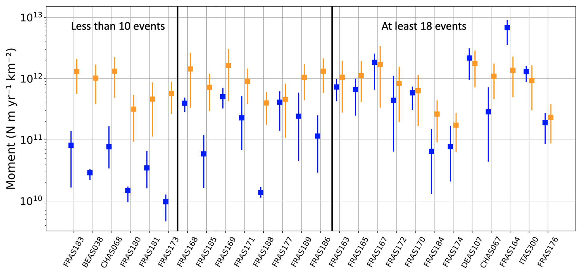
Figure 16 Comparison of geodetic moment rate (orange) and seismic moment rate (blue, inferred from the ESHM20 earthquake recurrence source model logic tree), for source zones in metropolitan France or on the border. Mean values and 16th and 84th percentiles. The order from left to right corresponds to an increasing number of events used for establishing the earthquake recurrence model, less than 10 events for sources FRAS183 to FRAS173, and 30 to 78 events for sources FRAS174 to FRAS176.

5 Conclusions

Many studies have been published that study how GPS strain rate is correlated with changes in observed seismicity (e.g., Zeng et al., 2018). Far less studies have focused on the comparison between strain rates and long-term earthquake forecasts built for assessing probabilistic seismic hazard. These long-term earthquake forecasts rely strongly on past seismicity, whereas geodesy offers an independent view on the amount of deformation that might be released in the future. In the present study, we have compared the new European seismogenic source model (Danciu et al., 2024) with a strain rate model developed at the European scale (Piña-Valdés et al., 2022). The comparison is led in terms of moment rates.

For every area source zone of the ESHM20 source model, we have established a distribution for the geodetic moment rate, which accounts for uncertainties in the selection of GNSS stations, the calculation of the strain rates, and the conversion into a moment rate. At the source zone scale, we compare the geodetic moment rate distribution with the seismic moment rate distribution, as inferred from the ESHM20 source model logic tree. We show that the geodetic moment rate is rather well-correlated with the seismic moment rate in the most seismically active regions of Europe (e.g., the Apennines, Greece, the Balkans, the Betics, southeastern France), whereas in the low-seismicity regions, the geodetic moment rate is much higher than the seismic moment rate (e.g., Parisian Basin, northern and central Europe, Fennoscandia). Results show that both estimates are slightly more consistent when considering larger spatial regions. In moderate- to high-seismicity regions, the geodetic strain is in general representative of the current horizontal tectonic stresses. In the very low seismicity region of Fennoscandia, the geodetic signal might be dominated by glacial isostatic adjustment, and the strain does not represent the long-term tectonic loading.

More work is needed to understand the consistencies or discrepancies obtained between strain-rate-based moments and moments relying on the long-term magnitude–frequency distributions built for PSHA. Some parameters such as the seismogenic thickness will need to be better evaluated to refine the estimation of the moment rate from strain rates. In regions of very low seismicity where the geodetic moment rate appears disconnected from the seismic moment rate, for now this is not clear how geodetic data can contribute to establish long-term earthquake forecasts. However, in seismically active regions, our work demonstrates the strong correlation between long-term seismic moment rates and geodetic moment rates. In these regions, strain rates should be used to constrain earthquake forecasts for PSHA, either combined with earthquake catalog data or as an alternative model independent of the earthquake catalog.