Subseasonal forecasts of heat waves in West African cities

Heat waves are one of the most dangerous climatic hazards for human and ecosystem health worldwide. Accurate forecasts of these events are useful for policy makers and climate services to anticipate the consequences of extreme heat. In particular, subseasonal forecasts are of great importance in order to implement actions to mitigate the consequences of extreme heat on human and ecosystem health. In this perspective, the present study addresses the predictability of heat waves at subseasonal timescales in West African cities over the period 2001–2020. The cities were grouped in three climatic regions based on their climate variability: the continental, Atlantic and Guinean regions. Two types of heat waves were analysed: dry heat waves using 2 m temperature and wet heat waves using average wet bulb temperature. Two models that are part of the subseasonal-to-seasonal forecasting project, namely the European Centre for Medium-Range Weather Forecasts (ECMWF) and the United Kingdom Meteorological Office models, were evaluated using two state-of-the-art reanalysis products, namely the fifth generation ECMWF reanalysis (ERA5) and the Modern-Era Retrospective analysis for Research and Application, Version 2 (MERRA-2). The performance of the forecast models in predicting heat waves is assessed through the computation of categorical metrics such as the hit rate, the Gilbert skill score and the false alarm ratio. The results suggest that at subseasonal timescales, the forecast models provide a better forecast than climatology, but the hit rate and false alarm rate are sub-optimal and the forecasts may be overestimating the duration of heat waves while under-predicting the intensity. Nevertheless, the use of subseasonal forecasts in West African cities can be recommended for prediction of heat wave onset up to 2 weeks in advance.

1 Introduction

The impact of heat waves on different sectors, in particular the economy and health, makes them one of the most dangerous climate hazards globally (Perkins, 2015). Heat waves pose a significant threat to human health, as they cause discomfort and stress to body temperature regulation. In some cases, heat waves can lead to various cardiovascular and respiratory diseases, increasing the risk of morbidity and mortality (e.g. Anderson and Bell, 2009; Gasparrini and Armstrong, 2011; Kovats and Hajat, 2008; Huynen et al., 2001). The combination of heat and humid atmospheric conditions can exacerbate heat stress and lead to deaths, particularly among vulnerable populations such as children and the elderly (Russo et al., 2017). The damage of heat waves on human health is amplified in urban regions due to the urban heat island effect. Over the last decades, West Africa cities were affected by several extreme heat events. In May 2013, the Senegalese town of Matam experienced a severe heat wave, with temperatures reaching 50 °C. This event, which persisted during the day and night, caused the deaths of 18 elderly people in 10 d. In the same period, Mauritania was affected by a devastating heat wave with maximum temperatures exceeding 46 °C, causing the deaths of more than 25 elderly people and children. Recently in April 2024, most African countries experienced extreme heat conditions. In Mali, for example, temperatures exceeded 48 °C, causing the deaths of more than 100 people.

Climatic projections show an increase in the frequency, intensity and duration of extreme temperatures over the next century and beyond (e.g. Kharin et al., 2007; Fischer and Schär, 2010; Perkins et al., 2012). Under these warming conditions, the frequency of extreme events such as heat waves will increase. In the latest Intergovernmental Panel on Climate Change report (IPCC report 2023), the authors show that equatorial regions will be more affected by climate change than mid- and high latitudes. This result from the IPCC is a warning bell, as the predictability of heat waves remains poorly documented in some equatorial regions, such as sub-Saharan Africa.

The impact of heat waves on human activities and health increases the need for skilful and reliable climate forecasts on subseasonal-to-seasonal timescales in order to anticipate risks and develop appropriate responses (Lowe et al., 2016). Therefore, early warning systems are of crucial importance to provide information on the occurrence of such events. Many early warning systems integrate short- and medium-range forecasts of potential weather hazards up to 2 weeks ahead. The subseasonal forecast range, from a 2- to 6-week lead time, is also highly relevant for actions aimed at mitigating the consequences of extreme heat (e.g. White et al., 2017; Moron et al., 2018; Tompkins et al., 2019; Osman et al., 2023). Subseasonal forecasts are used to monitor the evolution of specific weather patterns that have been identified in advance with seasonal forecasts. Subseasonal-to-seasonal (S2S) forecasts are of great importance for humanitarian services in order to build up a “ready, set, go” early warning concept that allows early actions to be taken before a potential disaster (e.g. Bazo et al., 2019; Lala et al., 2022; Domeisen et al., 2022).

Heat waves are often associated with extreme heat, which can be exacerbated by other factors such as humidity levels. A heat wave is defined as a period of unusual hot temperature over a region persisting for at least 3 consecutive days during the warm period of the year based on local (station-based) climatological conditions, with thermal conditions recorded above given thresholds (e.g. Perkins and Alexander, 2013; Déqué et al., 2017; Barbier et al., 2018; Batté et al., 2018; Ngoungue Langue et al., 2023). Many factors can affect the definition of a heat wave, including the end-user sectors (human health, infrastructures, transport, agriculture) and also the climatic conditions of the regions (Perkins and Alexander, 2013). Heat waves can be defined from daily meteorological variables, such as daily raw temperature (e.g. Batté et al., 2018; Lavaysse et al., 2018; Engdaw et al., 2022; Ngoungue Langue et al., 2023); minimum, mean and maximum daily wet bulb temperature (e.g. Yu et al., 2021; Ngoungue Langue et al., 2023); and heat stress indices (e.g. Robinson, 2001; Fischer and Schär, 2010; Perkins et al., 2012; Guigma et al., 2020; Ngoungue Langue et al., 2023), using relative or absolute thresholds. Heat stress indices are used to combine relevant atmospheric variables (such as temperature, humidity, solar and thermal radiation, wind speed) to indicate the impact of the environment on the human body. Examples include apparent temperature, the universal thermal climate index, excess heat factor (EHF) and excess heat index (EHI) (McGregor et al., 2015).

A few studies on heat wave forecasting have been carried out in West African regions. Batté et al. (2018) evaluated the predictability of heat waves during spring at subseasonal timescale using the Météo-France model as part of the S2S project. To assess the skills of the models, they used the apparent temperature and 2 m temperature (T2m) anomalies as indicators for heat wave detection. Apparent temperature represents the temperature actually felt by humans, caused by the combined effects of air temperature, relative humidity and wind speed. The results show that the Météo-France model is able to predict heat waves up to 1 week in advance. Guigma et al. (2021) assessed the predictability of Sahelian heat waves during spring at subseasonal timescale using the ECMWF extended-range forecasting system (ENS-ext), fifth-generation European Center for Medium-Range Weather Forecasts reanalysis (ERA5) and Berkeley Earth Surface Temperatures (BEST) gridded data for the evaluation. Their approach is based on the prediction of the probability of heat wave occurrence using T2m and heat index (HI) as indicators. They show that ENS-ext is able to forecast Sahelian heat waves with significant skill up to 2 weeks in advance, and with increasing lead time, wet heat waves (those combined with high humidity levels) are more predictable than dry heat waves (those combined with low humidity levels).

Batté et al. (2018) assessed heat wave predictability using T2m and AT anomalies. While this approach provides information about the evolution of T2m and AT for the subsequent days, it is not sufficient to determine heat wave characteristics such as the duration and frequency. In this study, we will adapt the methodology proposed by Lavaysse et al. (2019) when assessing the predictability of heat waves over Europe. This method offers a complete evaluation of heat wave characteristics including the evaluation not only of heat wave intensity, but also of heat wave onset and duration. It involves the computation of evaluation metrics to assess the skills of the models (see Sect. 2.5.3).

The present study assesses the subseasonal predictability of heat waves in West African cities over the period 2001–2020 using two models as part of the S2S project, namely the ECMWF and UKMO (United Kingdom Met Office) models. To the authors' knowledge, this work is the first of its kind in the region and represents a benchmark for future studies. To achieve our goal, we first analyse the representation of T2m and wet bulb temperature (Tw) in the forecast models with respect to the reanalysis data used as references (see Sect. 2). Secondly, we evaluate the models on the representation of extreme heat events and the spatial variability in heat wave characteristics. Finally, the skill of the models in predicting heat waves is evaluated.

The remainder of this article is organized as follows: in Sect. 2, we present the region of study and the data used for this work; the description of the methodology is also provided. Section 3 contains the main results of this study following the methodology presented in Sect. 2. Section 4 provides a discussion of the results, and Sect. 5 is dedicated to the conclusion.

2 Region, data and methods

2.1 Region of interest

This work is carried out for West Africa, covering an area between 5–20° N and 15° W–10° E, extending from the Atlantic coast to Chad and from the Gulf of Guinea to the southern fringes of the Sahara desert (Fig. 1). The climate of West Africa is mainly influenced by the West African monsoon, which regulates the rainy season and therefore affects agriculture. West Africa experiences a very hot and dry climate over the Sahel region and a hot and humid climate over the Guinean coast. The climatic conditions over West Africa and its location over the tropics expose the region to heat waves.

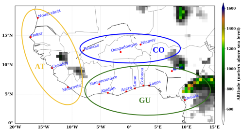
Figure 1 Topographic map of West Africa using ERA5 elevation data. The circles on the map represent the different climatic zones: AT (coastal Atlantic zone), CO (continental zone) and GU (coastal Guinean zone). The y and x axes represent the latitude and longitude respectively. The colour bar shows the elevation in metres over the region.

West Africa exhibits a high climate variability at regional and local scales. In this study, we focus on a few large, densely populated cities located in the Sahel region and on the Atlantic coast. The cities were grouped in three regions based on their location, climate variability and the evolution of heat wave characteristics in each region (Moron et al., 2016; Ngoungue Langue et al., 2023). The regions are structured as follows:

• The continental (CO hereafter) region includes the cities of Bamako, Ouagadougou and Niger (Fig. 1).

• The coastal Atlantic (AT hereafter) region includes the cities of Dakar, Nouakchott, Monrovia and Conakry (Fig. 1).

• The coastal Guinean (GU hereafter) region includes the cities of Yamoussoukro, Abidjan, Lomé, Abuja, Lagos, Accra, Cotonou and Douala (Fig. 1).

2.2 Reanalysis products

African cities suffer from a critical lack of weather observation stations, and the few that exist are not well distributed across the regions. Therefore, reanalysis data appear as good candidates to overcome this issue. We are aware that reanalysis data have a low resolution for detecting the highest temperatures at a point location, as well as the urban heat island effect. Nevertheless, reanalyses provide a numerical description of the recent climate by combining models with observations and are invaluable to numerous users around the world (Hersbach, 2016).

In this work, we use two state-of-the-art reanalysis products, namely the fifth-generation European Center for Medium-Range Weather Forecasts reanalysis (ERA5; Hersbach et al., 2020) and the Modern-Era Retrospective analysis for Research and Applications, Version 2 (MERRA-2; Gelaro et al., 2017), from the National Oceanic Atmospheric Administration (NOAA). In the following, we will use “MERRA” to refer to MERRA-2, which, along with ERA5, is one of the references for the evaluation of the forecast models. ERA5 and MERRA are part of the most reliable reanalyses used in African regions especially for the monitoring of heat waves (e.g. Barbier et al., 2018; Ngoungue Langue et al., 2021; Engdaw et al., 2022). Since ERA5 is used to initialize the atmospheric component of the ECMWF extended reforecasts, one could argue that the evaluation of the skills of the forecast models using only ERA5 as a reference is circular. For this reason, we have also included MERRA as a second reference. It also allows for estimating the uncertainties of the reanalyses.

2.2.1 ERA5

The ERA5 reanalysis provides hourly estimates of various climate variables for the entire globe using 137 hybrid sigma levels up to 80 km above the surface (Hersbach et al., 2020). The original spatial resolution is 0.28125°, interpolated to a regular 0.25°×0.25° grid. ERA5 outputs are generated by the CY41r2 model cycle of the Integrated Forecast System (IFS) of ECMWF, which uses a 10-member ensemble of 4D variational data assimilation. The set of atmospheric variables used within the ERA5 database are the hourly 2 m temperature (T2m) and hourly 2 m dew point temperature (d2m) covering the period from 1 January 2001 to 9 February 2021. From these variables, daily T2m (max, min, mean) and wet bulb temperature (Tw) are derived. The dataset is accessed through the Climserv database of the Institut Pierre Simon Laplace (IPSL) server or the Copernicus Climate Data Store (CDS). The land–sea mask used in this study was obtained from the ERA5 reanalysis and is available from the CDS.

2.2.2 MERRA

MERRA, unlike ERA5, has a spatial resolution of 0.625°×0.5° and provides data on 42 standard pressure levels. It uses an upgraded version of the Goddard Earth Observing System Model, Version 5 (GEOS-5), data assimilation system and the global statistical interpolation (GSI) analysis scheme of Wu et al. (2002). To ensure consistency in our analysis, we converted the MERRA data to a spatial resolution of 0.25°×0.25°, similar to ERA5 using a conservative first-order interpolation. In the MERRA database, we use the hourly T2m, hourly 2 m specific humidity and the pressure field at the surface from 1 January 2001 to 9 February 2021 to calculate daily T2m (max, min, mean) and Tw. The MERRA dataset was also accessed through the Climserv database on the Institut Pierre Simon Laplace (IPSL) server.

2.3 Forecasts products

To bridge the gap between medium range weather forecasts and seasonal forecasts, in 2013 the World Weather Research Programme (WWRP) and the World Climate Research Programme (WCRP) jointly launched a 5-year research initiative called the subseasonal-to-seasonal (S2S) project (Vitart et al., 2017) which aims to improve forecast skill and understanding on the subseasonal-to-seasonal timescale with special emphasis on high-impact weather events. The S2S project focuses on the risk of extreme weather conditions, including tropical cyclones, droughts, floods, heat waves and monsoonal rainfall (see http://www.s2sprediction.net/, last access: 19 December 2024). In order to obtain more robust statistical results, we conducted our study over a 20-year period, specifically using hindcast data from 2001 to 2020. Among the 12 models involved in the S2S project, we evaluated the ECMWF and UKMO models because they are both available throughout the study period.

2.3.1 ECMWF forecasts

The extended-range ECMWF forecast model used in this work is run on the IFS cycle CY47R3 released on 10 October 2021. The native spatial resolution of the ECMWF model is Tco639 L137 (about 16 km) up to day 15 and Tco319 (about 32 km) after day 15, but the downloaded data are interpolated to a regular 0.25°×0.25° latitude–longitude grid to match the resolution of ERA5 for evaluation. It contains 137 sigma levels from the surface to 80 km. ECMWF provides two types of outputs for the S2S project: forecasts and hindcasts. Hindcasts are forecasts produced for past dates and allow analysis of how the current system would have performed, alongside a consistent dataset covering a longer time period for evaluation. They are useful for the calibration of the model and post-treatment analyses.

The ECMWF extended-range hindcasts are run with 11 members (10 perturbed and 1 unperturbed). ECMWF extended-range hindcasts are produced twice a week, on Monday and Thursday, at 00Z. This means that for each week a new set of hindcasts is produced to calibrate the real-time ensemble forecasts for Monday and Thursday of the following week. We have only analysed the hindcasts produced on Thursdays, as a preliminary investigation into the initialization dates of the hindcasts showed that most models were launched on Thursdays. In the database, some models use fixed dates of the month (1st, 9th and 17th for example) and others specific days of the week (Monday and Thursday for example), which generate some difficulties to be handled. Most of the models do not cover the period under study except for UKMO, which is available but uses fixed initialization dates of the month (see section below for more details). It is therefore no longer possible to carry out a multi-model evaluation as we had planned, and we have limited the evaluation to ECMWF and UKMO. The ECWMF hindcasts produced on Monday cover the same period of the ones produced on Thursday. Thus, using the Monday hindcasts we have no significant changes in the frequency of the events detected. The 11-member ensemble hindcasts start on the same day and month as the forecasts but cover the last 20 years. In our case, the forecast year is 2021, and we focus on the previous 20 years from that date; the hindcasts run from 0–46 d. The variables of interest in the ECMWF S2S forecasts are T2m (max, min) over the last 6 h and daily average T2m and d2m, from which the daily average Tw was derived. The data are open access and available on the S2S project website (https://apps.ecmwf.int/datasets/data/s2s-realtime-instantaneous-accum-ecmf/levtype=sfc/type=cf/, last access: 19 December 2024).

2.3.2 UKMO forecasts

The UKMO model runs on the HadGEM3 GC2.0 model which simulates the uncertainties of the initial conditions using a lagged initialization and the uncertainties of the model using a stochastic scheme. The native spatial resolution of the UKMO model is N216 – 0.83°×0.56° (about 60 km at mid-latitudes) – but the downloaded data are extrapolated to a regular latitude–longitude grid of 0.25°×0.25°. It contains 85 vertical levels from the surface to 85 km and 4 soil levels: level 1 (0–0.1 m), level 2 (0.1–0.35 m), level 3 (0.35–1 m) and level 4 (1–3 m). Similar to ECMWF, UKMO provides forecasts and hindcasts to the S2S project. The UKMO hindcasts analysed here are run using the model version released in 2023 which produces seven members per cycle (six perturbed and one control) for the period 1993–2016 (no UKMO hindcasts available after 2016). They are produced four times per month, on the 1st, 9th, 17th and 25th. We are aware that these initialization dates are not the same as those of ECMWF, but we are interested in this work in the predictability of heat waves in a broad perspective and not on specific events. Our target period is from January 2001 to February 2021, and as mentioned earlier, the UKMO hindcasts are not available after the year 2016. To solve this problem and get more robust statistical results, we recomposed the products to obtain a new composite that covers the whole target period. The process applied is described in the following expression:

$$\begin{array}{}\text{(1)}& {\displaystyle }\begin{array}{rl}{\displaystyle }\text{T2m\_max}=& {\displaystyle }{\text{Hindcasts(T2m\_max)}}_{\mathrm{2001}-\mathrm{2016}}\\ {\displaystyle }& {\displaystyle }\bigcup {\text{Forecasts(T2m\_max)}}_{\mathrm{2017}-\mathrm{2021}}.\end{array}\end{array}$$

The forecasts were extracted for the same days as the hindcast initialization. In order to apply the concatenation over time between the hindcasts and forecasts, the coordinate dimensions of the two datasets must be the same. As shown above, the number of ensemble members in UKMO hindcasts and forecasts is completely different. Therefore, to meet this requirement, we reduced the number of ensemble members from seven to four (one control member and three perturbed members) in the hindcasts to match the number of ensemble members in the forecasts. We selected the three first perturbed members in the hindcasts over the seven available. The UKMO forecasts analysed in this work are launched for a 6-week duration. The variables extracted from the UKMO database are the same as those from the ECMWF. A summary of the main differences between the two models (ECMWF, UKMO) is provided in Table 1.

Table 1 Differences between the two forecast models.

2.4 Methods

2.4.1 Estimation of temperatures at the city scale from reanalyses

Weather forecasts provide the evolution of atmospheric variables on a global scale, which implies the need to have data from observation stations to access information on a local scale. This is a major problem in areas where there are not enough weather stations to collect data, as is the case in African cities.

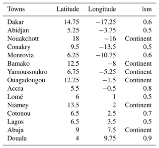
To address this issue, downscaling methods can be employed. However, in this study, we study phenomena at the city scale, and the spatial resolution of the reanalyses (ERA5, MERRA) is too coarse for this purpose. Although the reanalysis scale is more representative of the spatial variability of a heat wave occurring in a city than an isolated local station, a validation analysis is needed for test stations in order to determine the best interpolation technique for estimating local temperature from reanalyses. Following the same approach as in Ngoungue Langue et al. (2023), local temperatures over the cities were derived from the reanalysis using the reanalysis grid point closest to the station that satisfies a land–sea mask (lsm) of at least 0.5 (Table 2 shows the lsm values for all the cities considered in this study, and the same technique was applied for the forecast models). The lsm indicates the proportion of land contained in a grid point. If the lsm is less than 0.5, this means that the grid point is mainly covered by the ocean, while an lsm greater than 0.5 implies more land coverage.

Table 2 Land–sea mask (lsm) of West African towns used in this study.

2.4.2 Heat wave detection

In the present study, two types of heat waves are investigated: dry and wet heat waves. Dry heat waves are associated with high temperatures and low-humidity conditions. The detection of dry heat waves is processed using 2 m temperature (T2m) as an indicator. We distinguished two categories of dry heat waves: those that occur during the daytime and are detected using maximum values of T2m (T2m_max) and those that occur during the night and are detected using minimum values of T2m (T2m_min). Concomitant heat waves, those that occur during daytime and the night, are extremely dangerous because the body does not have the time to recover from the daytime heat waves during the night (e.g. Li et al., 2017; Wang et al., 2020a, b). The most lethal heat waves are due not only to high temperatures but also to the effect of humidity (e.g. Steadman, 1979a, b; Heo et al., 2019; Yu et al., 2021). Humidity is an important driver of wet heat waves. The combination of high heat and humidity can compromise the human body's main cooling mechanism: transpiration. The evaporation of sweat from skin cools our bodies, but higher humidity levels limit evaporative cooling. As a result, we can suffer heat stress and illness, and the consequences can even be fatal. Wet heat waves are detected here using average Tw as an indicator (Yu et al., 2021).

The computation of Tw is given by the following formula:

$$\begin{array}{}\text{(2)}& {\displaystyle }\begin{array}{rl}{\displaystyle }\text{Tw}=& {\displaystyle }T\cdot \text{atan}\left[A\right(\text{RH}+B{)}^{\frac{\mathrm{1}}{\mathrm{2}}}]+\text{atan}[T+\text{RH}]\\ {\displaystyle }& {\displaystyle }-\text{atan}[\text{RH}-C]+D\cdot (\text{RH}{)}^{\frac{\mathrm{3}}{\mathrm{2}}}\cdot [\text{atan}(E\cdot \text{RH})]-F,\end{array}\end{array}$$

where RH is used in percentage, for example, 40 for RH=40 %.

The computation of relative humidity (RH) varies depending on the available variables in the products. The first formula is applied for ERA5 (August, 1828; Magnus, 1844; Alduchov and Eskridge, 1996) and the second for MERRA (Ngoungue Langue et al., 2023) reanalyses:

$$\begin{array}{}\text{(3)}& \text{RH}=\mathrm{100}\cdot {\displaystyle \frac{\exp \left(\frac{a\cdot T_{\mathrm{d}}}{b+T_{\mathrm{d}}}\right)}{\exp \left(\frac{a\cdot T}{b+T}\right)}},\end{array}$$

$$\begin{array}{}\text{(4)}& \text{RH}=\mathrm{0.263}\cdot p\cdot q\cdot {\left[\exp \left({\displaystyle \frac{\mathrm{17.67}\cdot (T-T_{\mathrm{0}})}{T-\mathrm{29.65}}}\right)\right]}^{-\mathrm{1}},\end{array}$$

where a=17.625, b=243.04, A=0.151977, B=8.313659, C=1.676331, D=0.00391838, E=0.023101, F=4.686035, and T₀=273.16 K. Here T (°C), T_d (°C), T₀ (K), p (hPa) and q are respectively the ambient temperature, dew point temperature, reference temperature (water triple point temperature), pressure and specific humidity.

Daily maximum and minimum temperatures are computed respectively from maximum and minimum temperatures in the last 6 h. This choice of the computation of the extreme daily values is made according to the forecast models' outputs. Daily average wet bulb temperature is computed from hourly dew point temperature. This restriction to T2m_min, T2m_max and Tw is related to the atmospheric variables available for S2S outputs preventing us from computing more elaborate indices as in Ngoungue Langue et al. (2023).

We defined a heat wave as a consecutive period of at least 3 d during which the daily temperatures exceed the daily climatological 90th percentile computed over the entire period for T2m_min, T2m_max or Tw respectively (Fig. 2). The 90th percentile threshold is computed independently for the reanalyses and the hindcasts. As mentioned previously, the hindcasts are run at least once every week for a 6-week duration. For each initialization date within a month and for each lead time, we computed the daily climatological 90th percentile over the study period (2001–2020) (see Fig. S1 in the Supplement for an illustration of the computation of the 90th percentile threshold). Heat waves are detected independently for each initialization date within a month using the threshold values computed from this initialization (see Fig. S2 in the Supplement). For example, to detect heat waves in ECMWF hindcasts run on 4 January, the daily climatological 90th percentile of each day of the 4 January run is applied to each corresponding day of the runs on 4 January 2001, 4 January 2002, ..., 4 January 2020. The 90th percentile appears to be a sufficient threshold for monitoring heat waves affecting human health based on previous studies (e.g. Perkins and Alexander, 2013; Russo et al., 2014; Barbier et al., 2018; Lavaysse et al., 2019; Ngoungue Langue et al., 2023). Nevertheless, it is useful to determine the intensity of the events in order to establish a classification according to their severity (intensity), from “harmless” to “extremely dangerous”, for example (see Sect. 2.4.3 for more details on the computation of the intensity of heat waves).

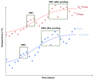
Figure 2 Detection process of heat wave: HW1 and HW2 represent events associated respectively to maximum and minimum temperature. The red and blue lines with circles are respectively maximum and minimum daily temperatures. Solid red and blue lines are respectively maximum and minimum thresholds. The x and y axes represent the time in days and the temperature in degrees Celsius. The term “after pooling” refers to the pooling of two (or more) events separated by a day characterized by the value of a given indicator below the daily XXth percentile. This figure is a “theoretical/schematic” illustration of the different types of heat waves investigated in this work.

The choice of a relative threshold is more appropriate as it is easily replicable in other regions. When two heat wave events are separated by 1 d with an indicator value below the daily 90th percentile on this day, they are pooled together to form a single event (Fig. 2).

2.4.3 Heat wave characteristics

After the detection of a heat wave, some important characteristics are deduced, namely the duration and the intensity. They are useful to investigate the severity of an event. The predictability of heat waves is assessed for occurrence, duration and intensity. To determine the occurrence and duration of heat waves, we create individual Boolean files from the T2m_min, T2m_max and Tw time series at each grid point, which is equal to 1 if it is a hot day and 0 otherwise. This operation is performed on a daily timescale over the study period. Hot days are days belonging to heat waves with the values of one of the three indicators (T2m_min, T2m_max or Tw) above their daily 90th percentile. In order to assess the characteristics of heat waves, only hot days belonging to heat wave sequences are considered (Ngoungue Langue et al., 2023). Boolean files are computed separately for reanalyses and forecasts in order to assess the representation of heat wave occurrence and duration.

The intensity of a heat wave was defined as the sum of the daily exceedances of the indicators' (T2m_min, T2m_max or Tw) values to a constant threshold for the duration of the event. It should be emphasized that this constant threshold is not used for heat wave detection but only to compute their intensity. In this study, which is part of the project Agence Nationale de la Recherche STEWARd (STatistical Early WArning systems of weather-related Risks from probabilistic forecasts, over cities in West Africa), we are interested in heat waves, which can be harmful to human health. Therefore, the constant threshold mentioned above is defined as the minimum of the daily climatological 90th percentile over the study period. The choice of a constant threshold for the computation of heat wave intensity is very important because it takes into account the seasonal cycle. This makes it possible to assess the severity of the events using the same reference. In fact, the most dangerous heat waves will have the highest intensity values.

2.5 Evaluation of heat wave forecasting in subseasonal models

Heat waves in the Sahel region occur mainly in spring due to the high temperatures in the region at that time (Barbier et al., 2018; Guigma et al., 2020). In this study, the region of interest was extended to the Guinean region in which heat waves are mainly driven by humidity coming from the Atlantic Ocean. This advection of humidity over the Guinean region is active during the season. Therefore, the detection of heat waves is performed over the whole season and not just in spring to cover the wet and dry seasons in the region. Similarly, the evaluation of the models is done from January to December for the different initialization dates independently by computing some statistical metrics. The metrics are computed for each week (week 1 to week 6) for each initialization date in a month, and the average score for each week is derived.

2.5.1 Evaluation of probabilistic forecasts

The representation of the evolution of T2m and Tw in ensemble forecasts is investigated by computing the bias between the subseasonal models and the reanalyses. To assess the predictive skills of the models in forecasting T2m, Tw and extreme heat events, we used probabilistic scores such as the continuous rank probability score (CRPS) and Brier score (BS).

The CRPS is a quadratic measure of the difference between the forecast and reanalysis cumulative distribution functions (CDFs); it quantifies the relative error between forecasts and observations. The values of the CRPS range from [0 to 1]: the closer it is to 0, the better the forecast. The CRPS is computed using the following formula:

$$\begin{array}{}\text{(5)}& \text{CRPS}=\underset{-\mathrm{\infty }}{\overset{+\mathrm{\infty }}{\int }}\left(P_{\mathrm{f}}\right(x)-P_{\mathrm{o}}{)}^{\mathrm{2}}\mathrm{d}x,\end{array}$$

where P_f and P_o represent the forecast and reanalysis CDFs respectively.

The BS measures the difference between the probability of a forecast and the outcomes; it is a good metric to quantify the accuracy of a forecast system. The BS is given by

$$\begin{array}{}\text{(6)}& \text{BS}={\displaystyle \frac{\mathrm{1}}{N}}\sum _{i=\mathrm{1}}^N(P_i-O_i{)}^{\mathrm{2}},\end{array}$$

where P_i and O_i are respectively the forecast probability and observed outcome (1 if the event occurs and 0 if not). N is the length of the forecast or observation time series.

2.5.2 From probabilistic to deterministic forecast

Ensemble forecasting is a tool used for making probabilistic weather forecasts. It is both an alternative and an indispensable complement to deterministic weather forecasts. Ensemble forecasting is of major interest because it provides different scenarios of the evolution of the state of the atmosphere. The particularity of ensemble forecasting is that, unlike deterministic forecasting, many trajectories are simulated in order to take into account uncertainties in the physical component of the model, the chaotic nature of the atmosphere, the observation network and imperfect initial conditions of the forecasts.

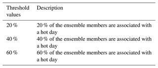
Although ensemble forecasting has many advantages over deterministic forecasting, the evaluation of the skills of an ensemble forecasting model remains quite complex due to the amount of information available. Statistical analyses can be performed by considering the ensemble mean, the median member, the warmest and coldest members, and the 1st and 3rd quartiles. Probabilistic scores exist for evaluating ensemble forecasting systems, but when it comes to the evaluation of specific events such as heat waves, the task becomes more complex. Moreover, probabilistic scores are difficult to understand for decision-makers and end users who are not specialists, hence the need to simplify and transform probabilistic forecasts into deterministic forecasts that are useful for implementing early warning systems. Our approach consists of converting ensemble forecasts into Boolean files using threshold values. Threshold values are defined as the percentage of members correctly forecasting heat wave days. Three threshold values were tested to find the optimal deterministic forecasts (see Table 3). Assuming a threshold of 20 % for example (i.e. that at least 20 % of ensemble system members are forecasting heat wave days), we determined the probability of the ensemble forecast systems predicting a day as being part of a heat wave. If the probability is greater than the threshold value, the day will be counted as “1” and “0” otherwise. The methodology used here and the choice of the selected thresholds are inspired by Lavaysse et al. (2019).

Table 3 Description of the threshold values.

2.5.3 Evaluation of deterministic forecasts

The predictability of heat waves in the forecast models is evaluated using dichotomous scores based on the coherence between reanalysis and forecasts such as hits, false alarms, misses and correct rejections. Let us consider a 2×2 contingency table (Table 4) from which three metrics have been computed: hit rate, false alarm ratio (FAR) and Gilbert skill score (GSS). The hit rate indicates the percentage of observed heat waves that have been correctly forecasted. The FAR gives the percentage of forecasted events that did not occur. The GSS measures the fraction of observed events that are correctly predicted, adjusted for hits associated with random chance (close to the climatology). Chance hits (CHs) are given as the event frequency multiplied by the number of event forecasts. The GSS takes into account the hits, misses and false alarms and neglects the correct rejections that would artificially improve the score. The values of the GSS range from [$-\frac{\mathrm{1}}{\mathrm{3}}$ to 1]; a GSS=0 indicates no skill, while GSS=1 is perfect skill. The GSS is computed using the following formula:

$$\begin{array}{}\text{(7)}& \text{GSS}={\displaystyle \frac{\text{hits}-\text{CH}}{\text{hits}+\text{false\_alarms}+\text{misses}-\text{CH}}},\end{array}$$

where CH is given by

$$\begin{array}{}\text{(8)}& \mathrm{\text{CH}}={\displaystyle \frac{(\text{hits}+\text{false\_alarms})(\text{hits}+\text{misses})}{\text{hits}+\text{false\_alarms}+\text{misses}+\text{correct\_rejections}}}.\end{array}$$

Table 4 Contingency table.

2.6 Heat wave forecast strategy

In this study, we adapted the methodology developed by Lavaysse et al. (2019) to evaluate the predictability of heat waves in the forecast models. This assessment is done in two steps:

• The first approach consists of determining the predictability of heat wave days in the forecasts with respect to the reanalyses. To do this, dichotomous scores (hits, false alarms, misses and correct rejection) have been computed for each day at different lead times from which the hit rate, FAR and GSS were derived. The scores are computed independently for each week and each city. This type of information is useful for early warning systems such as the STEWARd project.

• The second approach focuses on the predictability of the whole heat wave rather than hot days in the heat wave. Therefore, a heat wave occurring in the reanalyses is considered predicted by the forecast models if at least one hot day during the event is correctly predicted. To facilitate the evaluation, dichotomous scores are now computed for each week, and the hit rate, FAR and GSS are derived. For example, if a heat wave is detected in the reanalysis during the first week and a hot day within this heat wave is correctly predicted by the forecast model, then the heat wave is considered predicted and hit=1 and miss=0. We repeat the process over all weeks and calculate the hit rate.

3 Results

3.1 Assessment of skills in probabilistic forecasts

3.1.1 Climatology evolution of some atmospheric variables (T2m and Tw) in the forecasts and reanalyses

In this section, we investigated the representation of the climatological evolution of two key variables for this study, T2m and Tw, in the hindcasts with respect to the reanalyses. To do so, the seasonal climatological bias between the hindcasts and the reanalyses is computed over the 20-year period. The bias is computed for each set of coupled models (ECMWF–UKMO) and reanalysis (ERA5–MERRA) using T2m (min, max) and Tw values (Figs. 3 and 4 respectively)

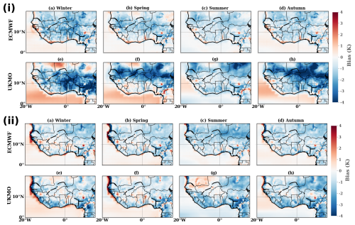
Figure 3 Spatial variability in the climatological bias between the forecast models' ensemble mean and ERA5 reanalysis over the period 2001–2020 for (i) T2m_min and (ii) T2m_max during the seasons (a, e) winter, (b, f) spring, (c, g) summer and (d, h) autumn. The bias is computed as the difference between the forecast models and ERA5 considering all the lead times. The colour indicates the bias values in degrees Kelvin. The x and y axes represent the longitude and latitude respectively.

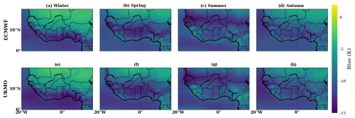
Figure 4 Spatial variability in the climatological bias between the forecast models' ensemble mean and ERA5 reanalysis over the period 2001–2020 for Tw during the seasons (a, e) winter, (b, f) spring, (c, g) summer and (d, h) autumn. The bias is computed as the difference between the forecast models and ERA5 considering all the lead times. The colour indicates the bias values in degrees Kelvin. The x and y axes represent the longitude and latitude respectively.

Firstly, we analysed the bias between the forecast models and ERA5 using T2m_min values. The range of biases associated with T2m spans −4 to 4 K. Both models show a negative bias with respect to ERA5 over the Sahel region which is more pronounced with UKMO (Fig. 3i). We noticed with UKMO a progressive shift in this strong negative bias over the northern Sahel during the season from winter to summer (Fig. 3i.e–g). The negative bias found in ECMWF over the Sahel region is consistent with previous global studies (e.g. Johnson et al., 2019; Haiden et al., 2021). The results obtained with T2m_max values are similar to those found with the T2m_min for both models. We especially notice a strong positive bias over the Atlantic coast during the winter and spring (Fig. 3ii.a, b and e, f). The evaluation of the representation of Tw in the hindcasts shows strong negative bias with respect to the reanalyses over the whole Sahel region (Fig. 4). In comparison to the results obtained with T2m, this strong negative bias can be linked mainly to the underestimation of humidity in the models in this region.

Secondly, we analysed the bias between the models and MERRA using T2m and Tw. We noticed significant discrepancies with the results obtained using ERA5 as a reference. Using T2m_min, we observed a positive bias in ECMWF with respect to MERRA over the Sahel and Guinean region during winter and autumn which tends to decrease during spring and summer. These results highlight the uncertainties between the two reanalyses already discussed in Ngoungue Langue et al. (2023). It can be deduced from these results using T2m_min that ERA5 has a warmer trend than MERRA over the Sahel region, while it is cooler than MERRA over the Atlantic Ocean (see Fig. S3 in the Supplement).

The spatial distribution of T2m and Tw in the forecast models shows significant biases with respect to the reanalyses. In order to determine whether these biases vary over time, we analyse the spatio-temporal evolution of T2m and Tw. The daily climatological biases are computed between the hindcasts and reanalyses over the CO, AT and GU regions at different lead times from week 1 to week 6. We observed a high spatial variability in the biases in the three regions. The models show smaller biases in the AT region in spring of the order of ±0.25 K, and larger biases of the order of ±2 K are found in the CO region with T2m_min (Fig. S4 in the Supplement). These large biases observed in the CO region are considerably reduced in summer. The results obtained with T2m_max are quite similar to those obtained with T2m_min (not shown). As observed in the previous results with Tw (Fig. 4), the models show lower negative biases in the CO region in winter (Fig. S5 in the Supplement). The range of biases associated with Tw spans −14 to 0 K. We do not observe any systematic increase in these biases from week 1 to week 6 (Figs. S4 and S5). This first assessment of the evolution of T2m and Tw in the models compared to the reanalyses reveals significant biases in the models which may lead to poor predictive skills.

3.1.2 Predictive skills of the models for T2m and Tw

This section addresses a global assessment of the skill of the models in the representation of T2m and Tw at different timescales. To do this, we analysed the interannual variability in the CRPS between the forecasts and reanalyses over the three regions for T2m_min, T2m_max and Tw. The CRPS values are in the same range for the first 2 weeks (week 1, week 2), the two intermediate weeks (week 3, week 4) and the last 2 weeks (week 5, week 6) (see Fig. S6 in the Supplement). According to these findings, we have chosen to organize our results into medium-range forecasts (week 2) and long-range forecasts (week 5). Week 5 was chosen for the long-range forecasts instead of week 6 because from week 5 onwards, the models generally reach the predictability horizon and are closer to the climatology. This organization of the results applies to the rest of the study.

The results of the CRPS computed using ERA5 as reference are shown in Fig. 5i. We have noticed that the skill of the models does not necessarily improve as the lead time decreases. This could be related to systematic biases in the forecast models (the representation of atmospheric circulation, local-scale processes). The CRPS score shows a high spatial variability in the three regions, indicating a high dependance of the skill of the models on the region. The forecast models show better predictive skills in the AT region during all the seasons and lead times with T2m_min except for UKMO during summer. The CRPS associated with T2m_max indicates that ECMWF is more skilful in the GU region (it is also the case with UKMO except during autumn when the AT region seems to be more predictable). In general, the models present higher skills for T2m_min than T2m_max over the AT region. ECMWF generally shows more skill than UKMO. The evolution of the CRPS computed using MERRA as a reference is similar to that found using ERA5 (not shown).

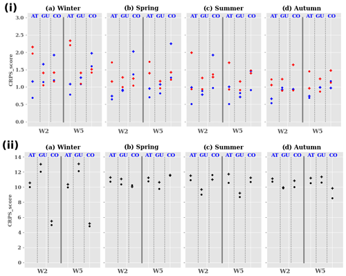
Figure 5 Evolution of the CRPS score between the forecast models and ERA5 reanalysis using T2m (i) and Tw (ii) over the period 2001–2020 during the seasons (a) winter, (b) spring, (c) summer and (d) autumn. The blue, red and black colours represent the CRPS score computed using T2m_min, T2m_max and Tw mean respectively. The CRPS is computed independently for each initialization date within a month, and we computed the average CRPS to obtain the CRPS values for the given month. The dot and cross symbols indicate the CRPS score obtained with ECMWF and UKMO respectively. The y and x axes show the CRPS values and the lead times (W2: week 2; W5: week 5) respectively.

We observed in the previous analyses (Fig. 4) a strong negative bias in the Sahel region with Tw; one could expect high CRPS values in the region. This is indeed the case, with CRPS values ranging from 4 to 13, i.e. 6 times higher than those obtained with T2_min or T2m_max. The CRPS values are drastically reduced in the CO region in winter, which is consistent with the previous results in Sect. 3.1.1 (Fig. 5ii). The models show more predictive skill in the representation of T2m than Tw. This is not surprising given that Tw combines T2m and humidity, which is very difficult to predict.

3.1.3 Predictive skills of the models for extreme temperatures

The representation of extreme heat events, referred to here as hot days (see Sect. 2.4.3), is evaluated in this section. This is done by the computation of the Brier score (BS) between the forecasts and reanalyses (ERA5, MERRA). The BS values obtained using ERA5 reanalysis as reference are very low between 0.05 and 0.175. We could think that the models show skills in forecasting hot days, but this is quite difficult to confirm because the BS is sensitive to the climatological frequency of an event: the rarer an event, the easier it is to get a good BS without having any real skill (https://www.ecmwf.int/sites/default/files/elibrary/2007/15489-verification-probability-forecasts.pdf, last access: 19 December 2024). This is actually the case with hot days which represent extreme temperatures. Using T2m, we found that in spring the models show less spatial variability than the other seasons (Fig. 6i). ECMWF performs better than UKMO in the detection of hot days except for Tw in the GU region in summer over all lead times, regions and seasons (Fig. 6ii). The results are similar with MERRA reanalysis (see Fig. S7 in the Supplement).

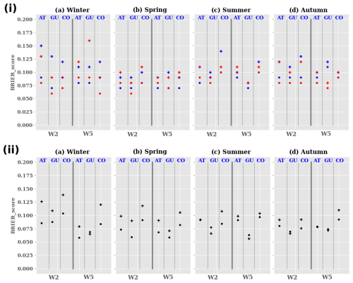
Figure 6 Evolution of the Brier score between the models and ERA5 reanalysis using T2m (i) and Tw (ii) over the period 2001–2020 during the seasons (a) winter, (b) spring, (c) summer and (d) autumn. The blue, red and black colours represent the Brier score computed using T2m_min, T2m_max and Tw mean respectively. The Brier score is computed independently for each initialization date within a month, and we computed the average Brier score to obtain the Brier score values for the given month. The dot and cross symbols indicate the Brier score obtained with ECMWF and UKMO respectively. The y and x axes show the Brier score values and the lead times (W2: week 2; W5: week 5) respectively.

3.2 Spatial variability in heat wave characteristics in deterministic forecasts

After assessing the skills of the models in predicting hot days, we study the spatial variability in heat wave characteristics in the forecast models with respect to the reanalyses. The frequency and characteristics of heat waves were computed using T2m and Tw. The mean duration and mean intensity of heat waves was computed for each grid point as the sum of respectively the heat wave duration and the intensity divided by the number of years affected by a heat wave during the period from 2001 to 2020. A first assessment of the representation of heat waves in the forecast models is done by computing the bias between the models and the reanalyses for heat wave frequency, duration and intensity. For this task, probabilistic forecasts are transformed into deterministic forecasts by computing the ensemble mean.

The spatial variability in heat wave frequency bias between the forecast models (ECMWF, UKMO) and ERA5 shows a similar evolution for T2m_min and T2m_max (Fig. 7). The models overestimate the frequency of heat waves in spring and summer over the Sahel for ECMWF and from the Sahel to the Guinean region for UKMO. This overestimation in heat wave frequency is well marked in UKMO, indicating the inaccurate representation of the daily variability in T2m in the model. The Sahel and Guinean regions exhibit strong convective activity during spring and summer which is very complex to take into account in the models. The representation of convective processes in the two models is assessed in the discussion in Sect. 4. Some discrepancies are observed in the spatial evolution of heat wave frequency when using Tw over the Guinean coast (Fig. 8); we noticed an underestimation in heat wave frequency over the Sahel and Guinean region in autumn.

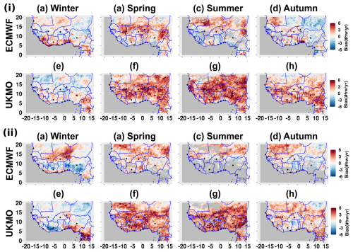
Figure 7 Spatial variability in heat wave frequency bias between forecast models and ERA5 over West Africa from 2001 to 2020 for (i) T2m_min values and (ii) T2m_max values during (a, e) winter, (b, f) spring, (c, g) summer and (d, h) autumn. The bias is computed as the difference in heat wave frequency between the forecast models and ERA5. This analysis is performed using the unperturbed member of the models and the forecasts over all the lead times. The colour bar indicates the bias values without units. The grey colour represents missing values. The x and y axes represent longitude and latitude respectively. The solid blue lines indicate the borders between countries; the black dots represent the cities of interest for this study (this applies to the rest of the paper).

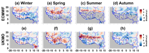
Figure 8 Spatial variability in heat wave frequency bias between forecast models and ERA5 over West Africa from 2001 to 2020 using Tw during (a, e) winter, (b, f) spring, (c, g) summer and (d, h) autumn. The bias is computed as the difference in heat wave frequency between the forecast models and ERA5. This analysis is performed using the unperturbed member of the models and the forecasts over all the lead times. The colour bar indicates the bias values without units. The grey colour represent missing values. The x and y axes represent longitude and latitude respectively.

In a second step, we assess the evolution of the number of heat wave days in the models versus ERA5. We observed a north–south gradient well established over West Africa and an overestimation of the number of heat wave days over the Guinean region for both T2m_min and T2m_max (Fig. 9). The north–south gradient is well marked in UKMO. This gradient observed in UKMO with T2m is also found in Tw and tends to strengthen from spring to autumn (Fig. 10). The main differences between T2m and Tw in the representation of heat wave days are found with ECMWF over the Guinean region. In winter, for example, there is an underestimation of the heat wave duration associated with Tw in the ECMWF model, while an overestimation is observed with T2m_min and T2m_max.

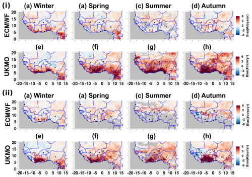
Figure 9 Spatial variability in heat wave duration bias between the forecast models and ERA5 over West Africa from 2001 to 2020 for (i) T2m_min values and (ii) T2m_max during (a, e) winter, (b, f) spring, (c, g) summer and (d, h) autumn. The bias is computed as the difference in heat wave duration between the forecast models and ERA5. This analysis is performed using the unperturbed member of the models and the forecasts over all the lead times during years when heat waves were detected. The colour bar indicates the bias values without units. The x and y axes represent longitude and latitude respectively.

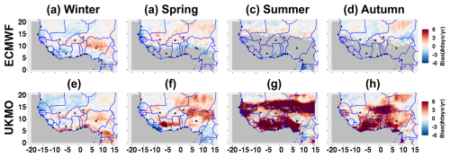
Figure 10 Spatial variability in heat wave duration bias between forecast models and ERA5 over West Africa from 2001 to 2020 using Tw during (a, e) winter, (b, f) spring, (c, g) summer and (d, h) autumn. The bias is computed as the difference in heat wave duration between the forecast models and ERA5. This analysis is performed using the unperturbed member of the models and the forecasts over all the lead times during years when heat waves were detected. The colour bar indicates the bias values without units. The x and y axes represent longitude and latitude respectively.

In a third step, the spatial evolution of heat wave intensity is evaluated. ECMWF generally tends to underestimate the intensity of heat waves over the Sahel region, while UKMO overestimates the intensity of events from the Sahel to the Guinean coast for T2m_min (see Fig. S8 in the Supplement). This overestimation of heat wave intensity in UKMO with T2m_min is considerably reduced when using T2m_max. The evolution of heat wave intensity with Tw is similar to that observed with T2m_min, except in summer for the ECMWF (see Fig. S9 in the Supplement). We found very similar patterns when computing the bias in intensity using MERRA reanalysis as reference for T2m_min, T2m_max and Tw (not shown).

The bias in heat wave duration using MERRA as reference shows some differences compared to results obtained with ERA5 reanalysis for both T2m_min and T2m_max (see Fig. S10 in the Supplement). The main differences are observed with T2m_max: during summer and autumn, ECMWF underestimates the number of heat wave days in the Sahel and Guinean region. This negative bias in heat wave duration appears in UKMO over the Guinean coast during summer and tends to extend over the Sahel in autumn (see Fig. S10ii). We do not find significant differences when using MERRA as reference for the evaluation of heat wave duration with Tw (not shown).

3.3 Assessment of the predictability of heat waves in deterministic forecasts

In this section, we investigated the skills of deterministic forecasts in predicting heat waves in the three regions. This is done by computing the following dichotomous scores described in Sect. 2.5.3: the hit rate, GSS and FAR (see Sect. 2). The scores are computed for T2m_min, T2m_max and Tw at daily and weekly timescales using the optimized forecasts (see Sect. 2) and ERA5 reanalysis chosen as reference. The evaluation of the forecast models at daily and weekly timescales provides useful insights for policy makers and climate services. Daily information is relevant for the accurate prediction of heat waves and early warning alert systems.

The results presented below are obtained using a 20 % threshold value to optimize the ensemble forecast systems (see Sect. 2.5.2) (Fig. 11). The hit rate and GSS values of the optimized forecasts using the thresholds 40 % and 60 % are lower than those obtained with the 20 % threshold. The hit rate values show a weak spatial variability in the three regions, which indicates that the skills of the models are not too sensitive to the topography and climatic characteristics of the three regions. We also noticed a gradual loss of predictability in the models from winter to autumn, with high hit rate values in winter. The forecast models show skills above the climatology both for medium- and long-range forecasts (week 2, week 5), but the hit rate values are very low, indicating misses in the forecasts. These results are not surprising, as we are interested in events that are extremely rare. The hit rate values are slightly better for medium-range forecasts. ECMWF presents higher skills than UKMO for medium-range forecasts in winter. UKMO, for instance, is better for long-range forecasts, mainly for T2m_min (Fig. 11i.a–d).

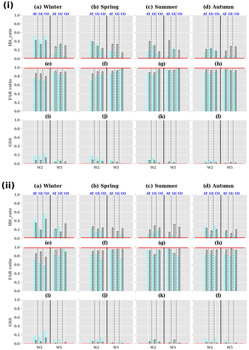
Figure 11 Evaluation of heat wave detection in the forecast models with respect to ERA5 at daily timescale over the period 2001–2020 using T2m_min (i) and T2m_max (ii) values for (a–d) hit rate, (e–h) FAR and (i–l) GSS. The metrics were computed using the optimized forecasts with the 20 % threshold (see Methods section for the optimization of the ensemble forecasts). The metrics are computed independently for each initialization date within a month, and all initializations are averaged to obtain the metric values for the given month. The metrics were grouped by seasons: (a, e, i) winter, (b, f, j) spring, (c, g, k) summer and (d, h, l) autumn. The cyan and black borders of bar plots indicate the metrics obtained when using ECMWF and UKMO respectively. The y and x axes show the metric values and the lead times (W2: week 2; W5: week 5) respectively. The horizontal red line represents the baseline climatology.

The models show higher skills in the AT and CO regions in winter and spring for T2m_min values for medium-range forecasts. In order to understand the behaviour of the models in these two regions, we investigated the inter-day variability in T2m by computing the standard deviation (SD) for each region using ERA5 reanalysis. We found small SD values in the AT and GU regions, indicating low variability in daily T2m in these regions (Table 5). Conversely, high variability in daily T2m is observed in the CO region. The low inter-day variability in T2m in the AT region indicates a more stable signal which will lead to favourable conditions for heat wave detection in the models based on a statistical perspective. Statistically, this will contribute to the occurrence of heat waves, as the probability of having consecutive days above the threshold is higher in a stable signal than in one with high daily variability. The skills of the models previously highlighted in the AT region could be partly explained by this low variability in daily T2m (min, max) in the region. The hit rate values obtained with Tw are very close to those associated with T2m in the different regions and seasons; but we also noticed with Tw that UKMO is more skilful than ECMWF for medium- and long-range forecasts (see Fig. S11a–d in the Supplement).

Table 5 Inter-daily variability in 2 m temperature over the period 2001–2020 using ERA5 reanalysis during the seasons (win, spri, sum and aut signify winter, spring, summer and autumn respectively) for T2m_min and T2m_max.

The second metric computed for the evaluation of the models is the GSS. The GSS follows the same evolution as the hit rate with much lower values between 0 and 0.2 for T2m_min, T2m_max and Tw (Figs. 11i.i–l, 11ii.i–l and S11i–l respectively). The highest values of the GSS are observed in winter. During winter, the atmospheric circulation in West African regions is mainly governed by the harmattan flow, which results in low convective activity in the regions and therefore an improvement in the predictive skills of the models compared to summer. The GSS values are positive, indicating that the forecast models perform better than the climatology mainly for medium-range forecasts (week 2) (Fig. 11i–l). Similar results of the GSS are found for Tw (see Fig. S11i–l).

An important parameter of a forecast system is its reliability in predicting events. “Do the events predicted by the models always occur in the reanalysis”? This is done by the computation of the false alarm ratio between the forecast models and ERA5 reanalysis for T2m_min (Fig. 11i.e–h), Tw (Fig. S11e–h) and T2m_max (Fig. 11ii.e–h). The FAR values are too high on average, about 0.7 and 0.85 for the medium- and long-range forecasts (week 2 and week 5) respectively for all three indicators. This suggests that the models tend to overestimate the number of heat days with respect to ERA5. The FAR increases with the lead time, and ECMWF issues fewer false alarms than UKMO for medium-range forecasts. The FAR is considerably reduced when we increase the threshold values used to optimize the ensemble forecasting systems (see Fig. S12 in the Supplement for T2m_min). This is highlighted more clearly in ECMWF than UKMO over all seasons and regions. This result is consistent with the fact that the prediction of an event will be more robust as a large number of model members have predicted the event. However, we found that this is not the case for the hit rate and GSS, for which high values are obtained with the lowest threshold (20 %) (see Figs. S13 and S14 in the Supplement). Thus, according to the context of the study, a compromise must be found in order to obtain a good balance between hit rate and false alarms.

The skill of the models in detecting heat waves is also assessed on a weekly timescale. As expected, we found an overall increase in the values of hit rate and GSS for T2m_min, T2m_max and Tw (see Fig. S15 in the Supplement for T2m_min).

The predictability of heat wave intensity in the models is also assessed for medium- and long-range forecasts (week 2 and week 5) using ERA5 reanalysis. We found a large spatial variability in heat wave intensity across regions. The strongest heat waves are found in the CO region (as shown in Ngoungue Langue et al., 2023) and low-intensity heat waves in the GU region except for Tw in summer for all three indicators. Although the models demonstrate consistency in forecasting the spatial distribution of heat wave intensity, they fail in accurately predicting the specific intensity values. The models underestimate the intensity of heat waves (see Fig. 12i for T2m_min; the results are very similar for T2m_max (Fig. 12ii) and Tw (not shown)). The forecast of heat wave intensity in the models remains a difficult task, even though the models show skills in heat wave detection.

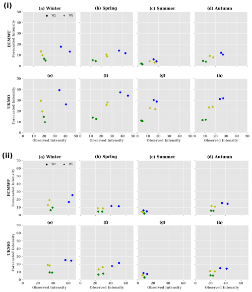
Figure 12 Evaluation of the intensity of heat waves in the forecast models and ERA5 over the period 2001–2020 during the seasons (a, e) winter, (b, f) spring, (c, g) summer and (d, h) autumn using T2m_min (i) and T2m_max (ii). The intensity of heat waves is computed independently for each initialization date within a month, and all initializations are averaged to obtain the average intensity of heat waves for the given month. Yellow, green and blue colours represent the values of intensity in the AT, GU and CO regions respectively. The dot and cross symbols represent the intensity of heat waves during week 2 (W2) and week 5 (W5) respectively. The y and x axes represent the forecasted and observed intensities in ERA5 reanalysis respectively.

4 Discussion

4.1 On the differences between the behaviour of forecasting models in different climatic regions

The behaviour of the forecast models varies across different climatic regions. The question that arises is why these differences exist. In order to tackle this question, we analyse some key factors in the models such as the physical parameterizations, the representation of the atmosphere–ocean coupling and the spatial resolution of the atmospheric model.

First of all, the physical parameterizations used to simulate atmospheric processes such as convection, turbulence, surface–ocean interactions, surface–radiation interactions and cloud microphysics are different for the two models. For example, for the representation of the convective activity, ECMWF is using the Tiedtke scheme (Tiedtke, 1989) and UKMO the Met Office convective scheme (Hagelin et al., 2017). The Tiedtke convection scheme is one of the first mass-flow convection schemes which aims to parameterize the effects of deep convection in numerical weather models. It simulates the vertical transport of heat, moisture and momentum associated with convective updraughts and downdraughts. The system takes into account various factors, including atmospheric instability, moisture content and boundary layer conditions to estimate convective processes. UKMO also uses a mass-flux convection scheme but one different from the Tiedtke scheme, which takes into account atmospheric instability and moisture content to determine convective activity. The difference between the two convective schemes could lead to an incorrect representation of convective activity in the region and thus limit the predictive skills of the models mostly for wet heat waves.

Secondly, the models use the same data assimilation methods (4D-Var) for control analyses, but the data and initial conditions are completely different. ECMWF assimilates a wide range of global and regional observational data, including satellite, radar and ground-based measurements. The UKMO focuses on observation data relevant to the United Kingdom and surrounding regions. The ECMWF atmospheric model is coupled with the NEMO3.4.1 ocean model, while UKMO uses the NEMO3.6 ocean model. The two systems are not using the same atmospheric and ocean models, which implies different parameterizations. The differences observed in the representation of T2m_min over the Atlantic Ocean (Fig. 3) could result from the representation of surface–ocean interactions in the models.

Thirdly, the spatial resolution of the atmospheric component of the two models is different: ECMWF has a higher spatial resolution than UKMO (0.32°×0.32° versus 0.83°×0.56°), which means that it can capture local-scale variability or atmospheric processes and provide more accurate forecasts for specific regions (https://confluence.ecmwf.int/display/S2S/ECMWF+Model, last access: 19 December 2024). Even if we transform the native resolution of the two models into a regular 0.25°×0.25° grid, some local-scale patterns will be found in the new grid. This may explain why the ECMWF performs better than the UKMO in some regions, for example in the case of extreme temperatures over the AT and GU regions (Fig. 6). A more detailed analysis of the influence of each factor on the results is beyond the scope of this paper.

4.2 On the skills of the subseasonal models at medium- and long-range forecasts

We noticed that in some regions, the CRPS score is slightly better during week 5 than in week 2, which is rather surprising. This behaviour is more apparent with UKMO; it is indeed the case in the Guinean region in January and February (see Fig. S16 in the Supplement). One first hypothesis on this behaviour in the UKMO model could be the strong seasonality in the region. Following this hypothesis, we investigate the seasonal evolution of the spread of temperatures in the Guinean region over the lead times. This investigation is very interesting because the variability in the spread can be linked to the skills of a forecasting model. We noticed higher spread values in winter compared to the rest of the seasons (see Fig. S17 in the Supplement). However, when we looked at week 2 and week 5, we did not find a specific evolution of the spread which can explain the behaviour observed in UKMO. The second hypothesis is the presence of a bias in UKMO which decreases over the lead times. Therefore, we analysed the evolution of the bias of temperatures over lead times. We found an intense cold bias of UKMO with respect to ERA5 over the Guinean region during winter. This intense cold bias could lead to high CRPS values in the region during winter (see Fig. S18 in the Supplement). The evolution of the bias during week 2 and week 5 shows similar patterns in January and February. This hypothesis on the bias evolution is not supported by these findings. One can suggest that atmospheric conditions and physical processes in the region during week 5 are well represented in UKMO compared to week 2. The investigation in more detail of the origins of this behaviour in the UKMO model is very complex and outside the scope of the present study.

5 Conclusions

This study is a first assessment of the predictability of heat waves in West African cities on a subseasonal timescale. Two models that are part of the S2S prediction project, namely ECMWF and UKMO, were evaluated using two state-of-the-art reanalysis data products, ERA5 and MERRA, over the period 2001–2020.

To carry out this study, we first analysed the representation of T2m and Tw in the forecast models with respect to the reanalyses. We found that the models are cooler than ERA5 in the Sahel region and hotter than MERRA in the Sahel and Guinean region. These uncertainties between the two reanalyses have also been highlighted in Ngoungue Langue et al. (2023).

Secondly, we assessed the spatial variability in heat wave characteristics. The models faced some issues in reproducing properly the spatial variability in the frequency, duration and intensity of heat waves. We found an overestimation of the frequency of heat waves in spring and summer over the Sahel for ECMWF and from the Sahel to the Guinean region for UKMO when using T2m. With Tw, we noticed an underestimation of heat wave frequency over the Sahel and Guinean region in autumn.

Thirdly, we investigated the predictability of heat waves in the models with respect to the reanalyses using dichotomous scores (hit rate, GSS and FAR). The hit rate and GSS values are very weak, while the FAR values are higher. On average, only approximately 15 % to 30 % of the predicted heat wave days are actually observed for week 5 and week 2 respectively. This suggests that the models overestimate the duration of the heat waves with respect to ERA5. ECMWF issues fewer false alarms than UKMO for medium-range forecasts. The detection of dry heat waves is slightly better with ECMWF for medium-range forecasts (week 2) during winter and spring, while it is better with UKMO for long-range forecasts (week 5) in the three regions. As far as wet heat waves are concerned, UKMO outperforms ECMWF for medium- and long-range forecasts. We are aware that the hit rate and GSS values are very low, but this is not surprising given that heat waves are extremely rare and difficult to predict because the persistence factor comes into play. Furthermore, we also know that the forecasting models underperform in tropical regions due to a poor representation of convective processes in their physical parameterization. Consequently, these scores, which are low but greater than the climatology, are significant for assessing the skill of the models in predicting heat waves in tropical regions, which remains a complex task. However the score are significant, the models underestimate the intensity of heat waves with respect to ERA5 at short-, medium- and long-range forecasts.

Regarding these results, we can recommend the use of subseasonal forecasts in African cities to predict the onset and frequency of heat waves as well as some days during the heat wave period at least 2 weeks in advance, but as far as their intensity is concerned, it is still challenging. Such information is very useful for the population, hospitals and decision-makers in order to develop some adaptation strategies to reduce the impacts of heat waves in the region.

In future work, we will investigate in more detail the origins of the differences observed in the two forecast models over the different regions. It has been shown recently in some studies that machine learning techniques can be useful in extending the predictability range of weather forecasts (e.g. Salcedo-Sanz et al., 2016; Anjali et al., 2019; Azari et al., 2022; van Straaten et al., 2023). Based on these findings, it would be interesting to investigate the potential of machine learning algorithms in heat wave forecasting.