Untangling the waves: decomposing extreme sea levels in a non-tidal basin, the Baltic Sea

Extreme sea level (ESL) events are typically caused by the combination of various long surface waves, such as storm surges and high tides. In the non-tidal, semi-enclosed Baltic Sea, however, ESL dynamics differ. Key contributors include the Baltic's variable filling state (preconditioning) due to limited water exchange with the North Sea and inertial surface waves, known as seiches, which are triggered by wind, atmospheric pressure, and basin bathymetry. This study decomposes ESL events in the Baltic Sea into three key components: the filling state, seiches, and storm surges. Our results show that storm surges dominate the western Baltic, while the filling state is more influential in the central and northern regions. Using a numerical hydrodynamic model, we further decompose these components based on their driving forces: wind, atmospheric pressure, North Atlantic sea level, baroclinicity, and sea ice. Wind and atmospheric pressure are the primary forces across all components, with the Atlantic sea level contributing up to 10 % to the filling state. These findings offer a deeper understanding of ESL formation in the Baltic Sea, providing critical insights for coastal flood risk assessment in this unique region.

1 Introduction

The threat of extreme sea level (ESL) events is escalating along the world's coastlines due to the rising mean sea level. This phenomenon is a leading cause of flooding in coastal areas, affecting more than 100 000 people annually in Europe alone. Moreover, this number is projected to rise in the future (Vousdoukas et al., 2020). Due to anthropogenic climate change, ESLs are projected to increase due to not only the rising mean sea level (e.g. Fox-Kemper et al., 2021) but also the intensification of tropical storms (e.g. Knutson et al., 2010) and changing sea level dynamics caused by sea level rise (e.g. Moftakhari et al., 2024), such as increasing tidal amplitudes and surges in estuaries (e.g. McGranahan et al., 2007; Talke et al., 2021) or in coastal lagoons (e.g. Bilskie et al., 2014; Lorenz et al., 2023).

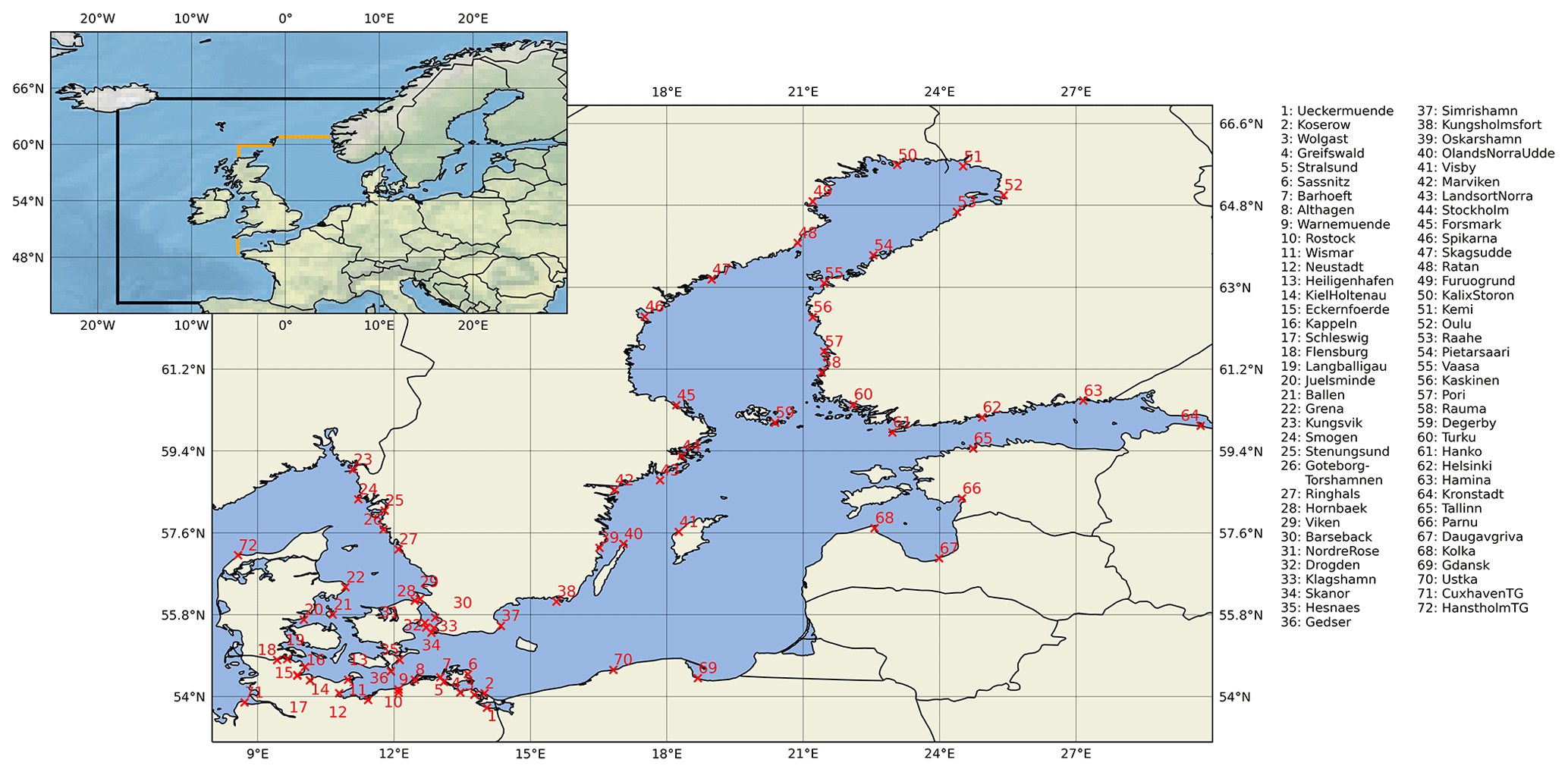
Figure 1 Model domain and station locations (red crosses and numbers) used for the temporal decomposition and model validation. The black line indicates the boundary of the coarse northwestern Atlantic Ocean domain. The orange lines mark the boundaries of the 1 nmi (nautical mile, 1 nmi = 1852 m) domain of the North Sea and Baltic Sea. Please note that Pietarsaari is also known as Jakobstad.

ESLs are often a combination of several processes, each leading to an increase in coastal sea level, e.g. high tides, storm surges, wave setup due to breaking wind waves, river discharge, and other surface waves. Storm surges occurring at high tide are the most common cause of ESLs in most coastal areas. For estuaries, where rivers flow into the sea, the coinciding of a storm surge at high tide with extreme river discharge poses a major flood hazard (e.g. Wahl et al., 2015; Hendry et al., 2019). Generally, when two or more extreme events co-occur, they are called compound events. Since many different components can contribute to ESLs, it is desirable to understand and quantify each to assess the risk and statistics of each contributor. However, decomposing ESLs is challenging. Using tide gauges alone, only a temporal decomposition is possible, e.g. the separation of tides and surges. However, non-linear interactions between the two complicate the separation (Idier et al., 2019; Arns et al., 2020), and they are, as a result, often neglected in impact studies (e.g. Rueda et al., 2017; Vousdoukas et al., 2018; Kirezci et al., 2020). Numerical models can allow the decomposition of ESL events into their different contributions, as individual processes and forcings can be switched on or off (Parker et al., 2023). In this way, each contributor can be quantified. Numerical models rely on good input data, such as atmospheric forcings with a good representation of storm systems, to capture storm surges and, hence ESLs, correctly. However, long-term, high-quality, and high-resolution reanalysis data that meet these requirements are often not available. Therefore, models are not always able to reproduce every individual event accurately. Nevertheless, a comparison with tide gauge data has shown that models can still correctly reproduce ESL statistics. Therefore, models are invaluable for the decomposition of ESL events into different components and forcings. Most decomposition studies assume a linear superposition of the individual sea level contributors (e.g. Parker et al., 2023). Interactions between the different contributors are often attributed to a residual term.

In this study, we follow the decomposition approach to analyse the ESLs within a non-tidal, semi-enclosed marginal sea, the Baltic Sea (Fig. 1). The Baltic Sea, located in northern Europe, has a mean depth of approximately 55 m. The region experiences postglacial isostatic land uplift of about 10 mm yr⁻¹ in the northern part of the sea, while the most southern region experiences subsidence of about 0.05 mm yr⁻¹ (Vestøl et al., 2019). Long-term global eustatic sea level rise in the Baltic Sea is not uniformly distributed across the region. It varies from 2 mm yr⁻¹ in the western part of the sea to more than 5 mm yr⁻¹ in the Gulf of Bothnia. About 75 % of the basin-averaged sea level rise can be attributed to the external sea level signal, while intensifying winds and poleward shifting low-pressure systems explain the spatial variation in the mean sea level trends (Gräwe et al., 2019). The prevailing winds are westerly to southerly (Bierstedt et al., 2015), and ESLs usually occur in autumn and winter when storm systems pass over the Baltic Sea region. A series of clustered storm systems can cause exceptionally high ESLs in the northern Baltic Sea due to the overlapping effects of previous storms (Rantanen et al., 2024). In the western Baltic Sea, very high sea levels have been observed in recent years (Groll et al., 2024), including the highest sea levels since 1872 in October 2023 (Kiesel et al., 2024). Events like these cause flooding, which will become more severe with sea level rise (Kiesel et al., 2023b), and pose problems for flood protection in the future (Kiesel et al., 2023a).

A recent review of the sea level dynamics and ESL events in the Baltic Sea has been compiled by Weisse et al. (2021) and Rutgersson et al. (2022) as part of the Baltic Earth Assessment Reports (BEARs). The sea level dynamics and the ESLs of the Baltic Sea have some unique contributions that distinguish the dynamics of the Baltic Sea from other coasts around the globe. First, the Baltic Sea has negligible tides (e.g. Gräwe and Burchard, 2012). In addition, since the Baltic Sea is separated from the North Sea by the shallow and narrow Danish Straits, water exchange between the Baltic Sea basin and the North Sea is hindered. The Danish Straits effectively act as a low-pass filter, filtering out high-frequency surface waves, such as storm surges and tides, from the North Sea. On the other hand, the slow water exchange on the timescale of a week or longer determines the mean sea level of the Baltic Sea, also called the filling state or, in the context of ESL events, the preconditioning (Leppäranta and Myrberg, 2009; Madsen et al., 2015). This exchange is mainly controlled by the westerly winds (Gräwe et al., 2019). Similarly, local preconditioning in sub-basins can contribute to ESLs, e.g. up to 1 m in the Gulf of Riga (Männikus et al., 2019). Although the Baltic Sea has negligible tides, there are basin-wide inertial surface waves with fixed frequencies between (13 h)⁻¹ and (44 h)⁻¹, which are given by the basin geometry (e.g. Wübber and Krauss, 1979; Zakharchuk et al., 2021). These inertial waves are called seiches and are excited by perturbations in the sea level. Their amplitudes can be as large as 17 cm, although their initial perturbations are smaller (Zakharchuk et al., 2021). Together with storm surges, these three temporal components (filling, seiches, and storm surges) are the main contributors to ESL events. At the coast, local sea levels may be directly elevated by wind-driven wave effects, such as wave setup (Su et al., 2024) or wave run-up. Meteotsunamis can be an additional component (Pellikka et al., 2020, 2022). Due to local geometries and orientations of the coastal topography, different regions are susceptible to different combinations of compounding contributions. Therefore, the return levels of ESLs are very heterogeneous. The return levels for a 30-year ESL event range from 0.7 to 2.5 m a.m.s.l. (metres above mean sea level) (Lorenz and Gräwe, 2023a), with the highest ESLs occurring at the head of the Gulf of Finland, in the Gulf of Riga, and in the western Baltic Sea (Wolski et al., 2014; Wolski and Wiśniewski, 2020). The historical storm surge of 1872 reached sea levels of more than 3 m in the western Baltic Sea (e.g. Hofstede and Hamann, 2022), with an estimated return period of about 1000 to 3000 years, depending on the location and the statistics (MacPherson et al., 2023). This event resulted from very high preconditioning and an exceptionally high storm surge, which could have been even higher (Andrée et al., 2023). Another event was recorded in 2005 in the Gulf of Riga, with a maximum sea level of 2.75 m at Pärnu (Suursaar and Sooäär, 2007; Mäll et al., 2017). Historical events like these are often considered statistical outliers that do not seem to belong to the main population of extreme events (Hofstede and Hamann, 2022; Suursaar and Sooäär, 2007). However, their inclusion in the statistics is beneficial, as they can significantly change the sea level design for coastal protection (MacPherson et al., 2023).

Storm surges are driven by winds and air pressure, the primary forces acting on the sea surface. However, the enclosed nature of the Baltic Sea limits the distance over which the momentum for storm surges can be deposited. Additionally, the northern Baltic Sea is partially covered by sea ice from winter to spring (e.g. Luomaranta et al., 2014). Sea ice acts as a lid, hindering the transfer of momentum from the wind to the water and reducing the ESLs by several decimetres (Zhang and Leppäranta, 1995). These factors, combined with short fetch lengths, generally result in lower return levels for the Gulf of Bothnia, except at its northern head where the fetch length is maximal for southerly winds (Wolski et al., 2014; Lorenz and Gräwe, 2023a).

Among all the contributors to ESLs in the Baltic Sea, this study quantifies the contributions of the filling or preconditioning, seiches, and storm surges to ESL events by performing a temporal decomposition. The second focus is quantifying the relative importance of the different forcings on the ESL events by performing numerical simulations. We quantify the role of the following forcings: wind, air pressure, North Atlantic sea level, baroclinicity, and sea ice.

2 Data and methods

2.1 Observational gauge data

The observational tide gauge data are obtained from the European Marine Observation and Data Network (EMODnet; https://emodnet.ec.europa.eu, last access: 5 June 2021) and the Global Extreme Sea Level Analysis (GESLA; Woodworth et al., 2016; Haigh et al., 2022). Both data sources provide quality-controlled sea level data at an hourly frequency and with high accuracy (1 cm). We have selected over 70 stations (see Fig. 1 for their locations) to (i) study the temporal decomposition of the observed ESL events and (ii) validate the modelled ESL events to ensure that the temporal decomposition agrees with the observations. Before any analysis, we selected the years 1961 to 2018 (the same time period covered by the model run; see next section) and subtracted the long-term linear trend of the mean sea level for each tide gauge. De-trending removes the mean sea level rise and glacial isostatic adjustments (GIAs; Peltier, 2004) from the time series. Note that some gauges have records shorter than the time period considered and many contain temporal gaps (Lorenz and Gräwe, 2023a).

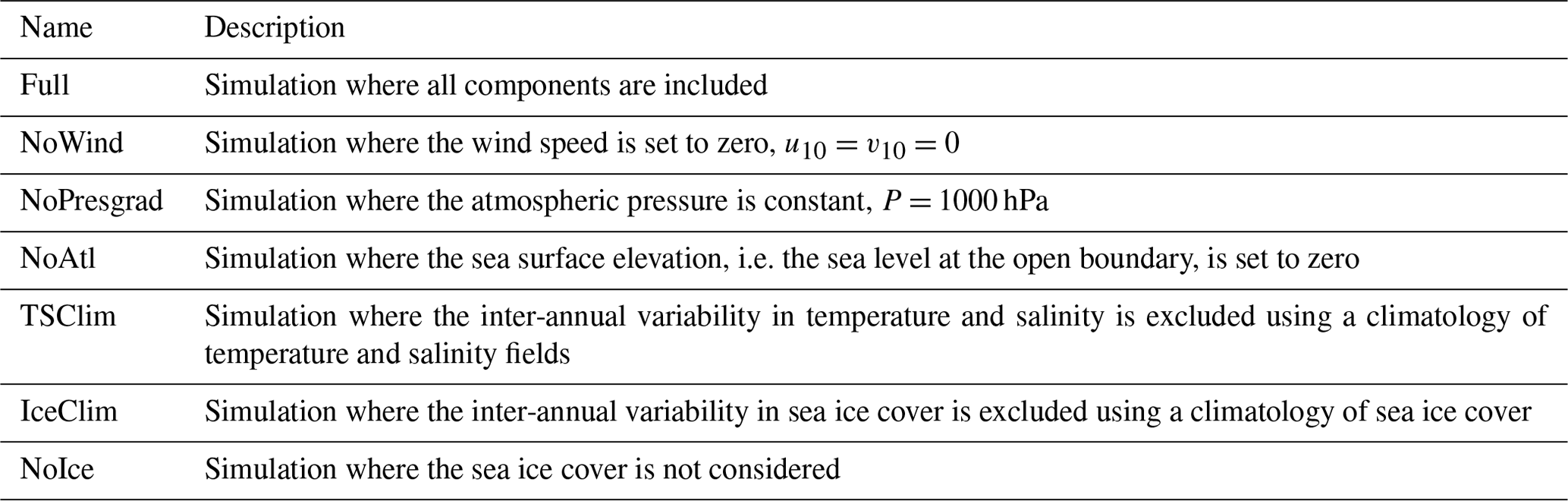
Table 1 Overview of the different simulations performed in this study.

2.2 Numerical simulations

We use the General Estuarine Transport Model (GETM, version 2.5; Burchard and Bolding, 2002) to simulate the sea level dynamics of the Baltic Sea. GETM has been used to model the hydrodynamics of several marginal seas and estuaries around the world. It has successfully demonstrated its ability to capture the complex hydrodynamics of the Baltic Sea (Gräwe et al., 2015), the mean sea level dynamics of the Baltic Sea (Gräwe et al., 2019), and its extreme sea levels (Lorenz and Gräwe, 2023a; Kiesel et al., 2023a). The model configuration is the same as in Lorenz and Gräwe (2023a) for their ensemble member UERRA (baroclinic) (Uncertainties in Ensembles of Regional ReAnalyses). The configuration uses a model chain starting in the northwestern Atlantic (5 nmi resolution, bottom roughness of z₀ = 5 mm) to generate boundary conditions for the North Sea and Baltic Sea domain (1 nmi resolution, bottom roughness of z₀ = 1 mm, Fig. 1; see e.g. Gräwe et al., 2015). Along the boundary of the northwestern Atlantic domain, air-pressure-induced sea level changes (the inverse barometric effect) are prescribed by the ERA5 reanalysis (Hersbach et al., 2020), which is also used as the atmospheric forcing for this setup. In this way, large pressure systems over the Atlantic are included in the model chain. The North Sea and Baltic Sea setup is forced by Uncertainties in Ensembles of Regional ReAnalyses (UERRA; Ridal et al., 2017), where the winds are increased by 7 % to better represent the ESLs in the western Baltic Sea (Lorenz and Gräwe, 2023a). The spatial resolution of the UERRA forcing is 11 km, and the temporal resolution is hourly. Tides are not considered, as they are negligible in the Baltic Sea. Static monthly mean density fields and sea ice cover are obtained from Gräwe et al. (2019). Wind stress reduction by sea ice is considered as in Gräwe et al. (2019). The advection scheme is the Superbee TVD (total variation diminishing) scheme (Pietrzak, 1998). The simulation period is 1961 to 2018. We save sea level data in a time step of 20 min.

We exclude different forcing components in different model simulations to investigate their effects on the sea level (see Table 1), i.e. seven simulations during the period from 1961 to 2018. The difference respective to the Full simulation, where all components are included (the same model simulation as used by Lorenz and Gräwe, 2023a), is then attributed to the effect of the excluded forcing. A detailed description of the decomposition approach is presented in the following sections.

2.3 Decomposition approach

2.3.1 Temporal decomposition

We first split the time series of sea level elevation into three contributions: the surge η_surge, the filling state of the Baltic Sea η_fill, and the seiches η_seiche:

$$\begin{array}{}\text{(1)}& {\mathit{\eta }}_{\text{ESL}}={\mathit{\eta }}_{\text{surge}}+{\mathit{\eta }}_{\text{fill}}+{\mathit{\eta }}_{\text{seiche}}.\end{array}$$

ESL events η_ESL are identified by applying a peak-over-threshold method. The threshold is determined by the 99.7th percentile of the time series, and we only consider events that are separated by more than 48 h (Arns et al., 2013). The filling state η_fill is computed by applying a Butterworth low-pass filter with a cut-off frequency of 7 d, corresponding to the weekly timescale described by Soomere and Pindsoo (2016) and Pindsoo and Soomere (2020). This timescale includes both the average filling state of the whole Baltic Sea and the local filling due to persistent winds such as storm systems. To extract the seiche contribution η_seiche from the time series, we consider a time window of ± 7 d around the peak sea level and force a fit of fixed frequency oscillations f_i:

$$\begin{array}{}\text{(2)}& {\mathit{\eta }}_{\text{seiche}}=\sum _i{a}_i\sin ({\mathit{\omega }}_{i}t-{\mathit{\varphi }}_i),\end{array}$$

where i denotes the index of the frequencies considered; a_i and ϕ_i are the fitted amplitude and phase lag of the seiche, respectively; and ω_i=2πf_i. For the Baltic Sea, the dominant frequencies f_i that we consider are (13 h)⁻¹, (23 h)⁻¹, (25 h)⁻¹, (27 h)⁻¹, (29 h)⁻¹, and (41 h)⁻¹ (Wübber and Krauss, 1979; Zakharchuk et al., 2021). Note that even more frequencies could have been added, but the amplitudes of these frequencies are much smaller. In addition, since we are considering 𝒪(100) events per station, the uncertainty estimates based on these statistical samples will be larger than the missing frequency contributions. Therefore, the errors introduced by neglecting these additional frequencies are expected to be negligible for this study. The surge component is then computed using

$$\begin{array}{}\text{(3)}& {\mathit{\eta }}_{\text{surge}}={\mathit{\eta }}_{\text{ESL}}-{\mathit{\eta }}_{\text{fill}}-{\mathit{\eta }}_{\text{seiche}}.\end{array}$$

This temporal decomposition is done for both observed and modelled ESLs.

2.3.2 Decomposition into forcing contributions

In addition to the temporal decomposition, we assume that each contributor in Eq. (1) can be linearly decomposed as the sum of the sea levels driven by the forcing components, namely wind η_wind, air pressure η_pres, sea level of the Atlantic η_Atl, inter-annual variability in the baroclinic velocities due to seawater density gradients η_barocl, sea ice η_ice, and the inter-annual variability in the sea ice cover η_{icevariability}:

$$\begin{array}{}\text{(4)}& \begin{array}{rl}{\mathit{\eta }}_j=& {\mathit{\eta }}_{j,\text{wind}}+{\mathit{\eta }}_{j,\text{pres}}+{\mathit{\eta }}_{j,\text{Atl}}+{\mathit{\eta }}_{j,\text{barocl}}+{\mathit{\eta }}_{j,\text{ice}}\\ & +{\mathit{\eta }}_{j,\text{icevariability}}+{\mathit{\eta }}_{j,\text{res}},\end{array}\end{array}$$

where j denotes surge, filling, and seiche. Since there are interactions between the sea levels that are driven by the different contributors, we have included the residual term η_res, which essentially represents the difference between η_j and the sum of the sea level contributions on the right-hand side, excluding the residual term itself. To extract the effect of each forcing, we subtract each simulation where we have excluded one component from the Full simulation (compare to Table 1). For example, the time series of the sea level evolution due to wind forcing is computed by

$$\begin{array}{}\text{(5)}& {\mathit{\eta }}_{\text{wind}}={\mathit{\eta }}_{\text{Full}}-{\mathit{\eta }}_{\text{NoWind}}.\end{array}$$

The other forcing contributions are computed accordingly.

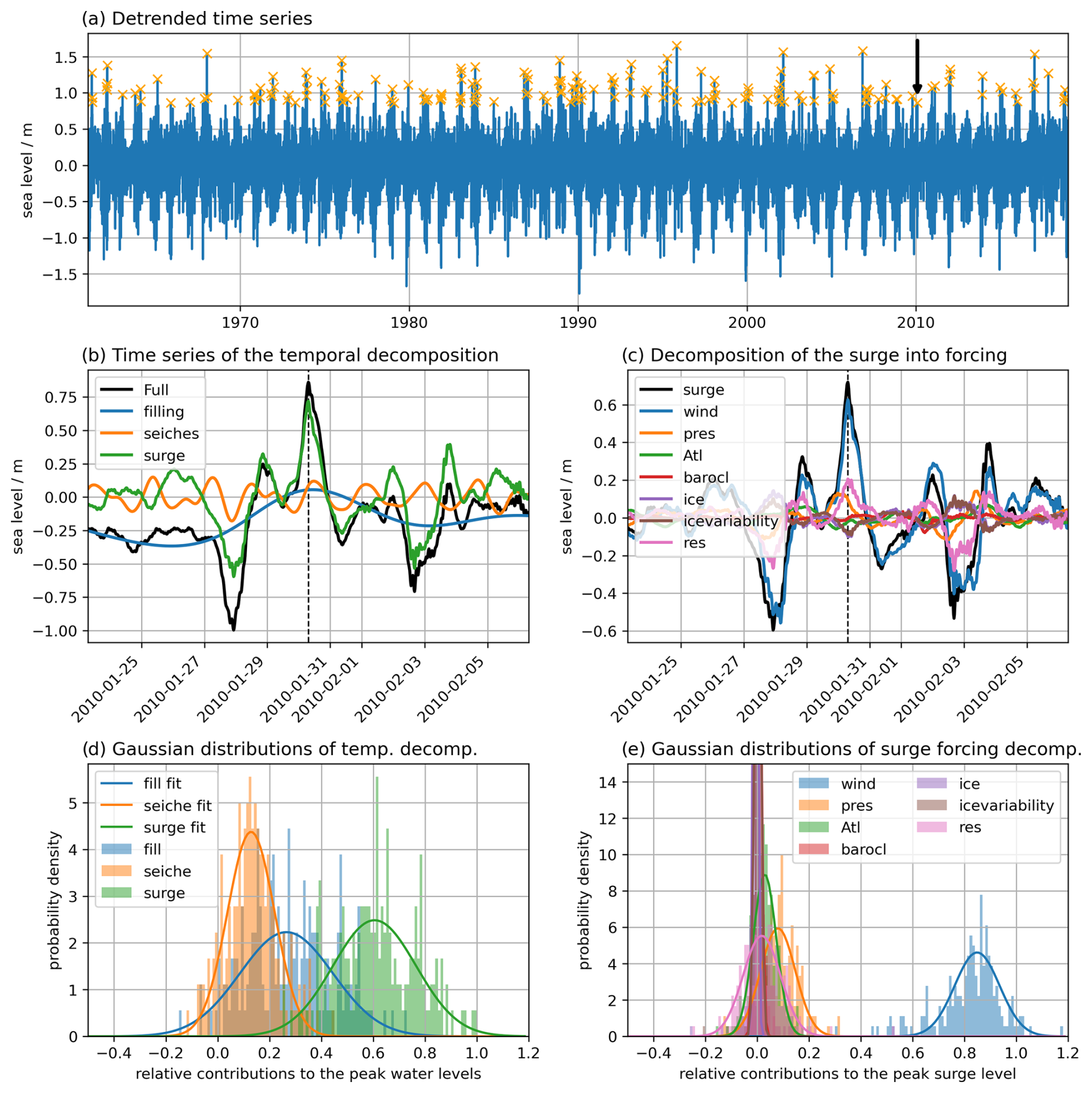
Figure 2 Exemplary results of the workflow for the decomposition of ESL events. (a) The de-trended time series of the Warnemünde station. The orange crosses indicate all ESL events considered. The black arrow denotes the exemplary event that is decomposed in panels (b) and (c). (b) Temporal decomposition into the filling, seiche, and surge components around the peak sea level of the event. (c) Decomposition of the surge component into the different forcings. The dashed black line in (b) and (c) marks the time of the peak sea level. (d) The histograms and fitted Gaussian distributions of the temporal decomposition using all the events marked in (a). (e) Similar to (d) but for the decomposition into forcing contributions for the surge component.

2.4 Workflow of the time series analysis

As a first step, the long-term changes in the mean sea level are removed from the time series by de-trending (by subtracting the linear trend of the entire time series; see Fig. 2a). The filling time series η_fill is then computed by applying the Butterworth low-pass filter with a cut-off frequency of 7 d, as mentioned previously. ESL events are identified in the de-trended time series by applying a peak-over-threshold method. The threshold is determined by the 99.7th percentile of the time series, and we only consider events that are separated by more than 48 h (Arns et al., 2013). For the modelled time series spanning the 58 years from 1961 to 2018, approximately 80 to 250 events are identified for each station. The station locations are shown in Fig. 1. The number of events in the observed time series may differ due to the varying lengths of the time series and data gaps. Note that the search for ESL events is only performed for the Full simulation.

We consider a time slice of ±7 d for each event around the peak sea level. From the resulting shorter time series, each filling is first subtracted. Then, the seiches are force-fitted with Eq. (2) followed by the computation of the surge component with Eq. (3). An exemplary temporal decomposition of the Warnemünde time series (Fig. 1, station 9) is shown in Fig. 2b. For each temporal component, we record the sea level occurring at the time of the peak sea level (dashed line in Fig. 2b). This results in a sample of sea levels for the total peak level and its respective components from the temporal decomposition. In addition, the maximum filling and maximum seiche level values within a 48 h window, i.e. ± 24 h around the ESL peak, are stored to assess the potential ESL if all three components were to reach their peaks simultaneously.

To study the relative importance of each component, the components are normalized to the peak level for each event and stored in a histogram with a bin size of 0.01, ranging from −0.5 to 1.2. The normalization allows us to utilize all events to make a general statement about the mean composition of ESLs. Each histogram is used to fit a Gaussian distribution to extract the mean and standard deviation; see Fig. 2d. For this station, the mean temporal contributions are 60.5 % surge, 26.5 % filling, and 12.9 % seiche (a sum of 99.9 %). Similar to the methodology described, each temporal component, filling, seiche, and surge, is decomposed into the contributions of the different forcings, as shown in Fig. 2c and e for the surge component as an example. Since the sea ice component can only lower the sea level, the Gaussian fit approach is unsuitable due to its non-Gaussian distribution. Therefore, for the sea ice component, the mean and standard deviation are computed directly from the sea levels and then normalized. For Warnemünde station, the mean forcing contributions are 84.5 % wind, 8.0 % air pressure gradients, 2.9 % Atlantic sea level, 0.2 % baroclinicity of seawater, −0.5 % sea ice, 0.2 % sea ice variability, and 1.8 % residual (a sum of 97.1 %). Due to the uncertainty in the fits, we cannot expect the sum of all forcings to add to 100.0 %.

Note that the distribution of ESLs generally follows a tail-end statistical distribution, such as the generalized extreme value or generalized Pareto distribution. The filling component follows a classical asymmetric quasi-Gaussian distribution (Soomere et al., 2015). However, as we generate samples of relative contributions to normalized peak sea levels, these samples are expected to follow a Gaussian distribution (except for the sea ice component).

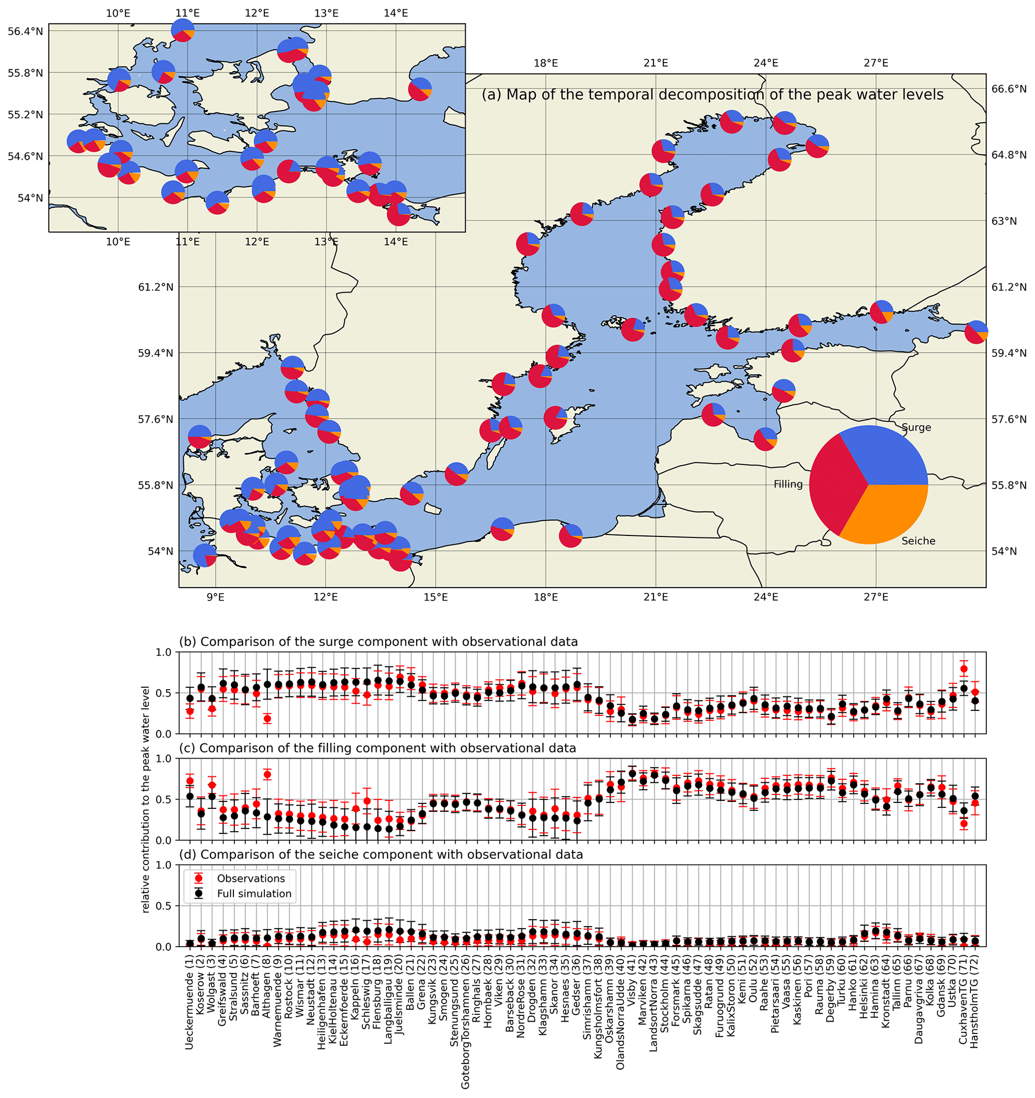
Figure 3 Temporal decomposition of the peak sea levels. (a) Map of the temporal decomposition of the ESL events in the observations from each station. (b) Comparison of the modelled surge component with the surge component from the observed sea level data. The mean (dots) and standard deviation (caps) are obtained from the Gaussian distribution fits (except for sea ice simulations; see Sect 2.4 and compare to Fig. 2d). (c) As (b) but for the filling component. (d) As (b) but for the seiche component.

3 Results

3.1 Temporal decomposition

The temporal decomposition of the observed ESLs indicates that in the western Baltic Sea, the surge component accounts for more than 60 % of the ESL events for all stations (Fig. 3a and b). Following the surge component, the seiche and filling components contribute almost equally. For the westernmost stations, the seiche contribution exceeds that of the filling. In contrast, stations located along the eastern German coast show a greater contribution of the filling component, indicating that these stations are closer to the seiches' pivot point(s) and, therefore, experience smaller seiche amplitudes. Note that the seiche periods of 23 to 29 h are in the range of the duration of the surge events in this region of the Baltic Sea (Kiesel et al., 2023b). Along the southwestern coast of the Baltic Sea towards Sweden, the largest contribution shifts from the surge to the filling component. The filling component contributes 50 % to 75 % of the total ESL along the coasts of the Baltic proper and the Gulf of Bothnia (Fig. 3a and c). For most of the Swedish coast, the remaining contribution to the ESL is the surge component, with almost negligible seiches (Fig. 3a and d). A similar pattern is found on the Finnish coast in the Gulf of Bothnia. In the Gulf of Finland, the surge is the second-largest contributor followed by the seiche component, with the filling component remaining the largest contributor. The surge component becomes more significant when a tide gauge is located further east in the Gulf of Finland due to the increased fetch length over which the wind can transfer momentum to the sea. In the Gulf of Riga, the seiche component is again negligible, and the contribution of surges to the ESLs is nearly as significant as that of the filling. For the Polish stations, Gdańsk and Ustka, the decomposition is similar to that of the Gulf of Riga, with almost negligible seiches.

Comparison of the gauge data decomposition with the numerical model results (Fig. 3b–d) shows that the model statistics agree with the observed statistics. Differences are found for gauges that are located within coastal lagoons or estuaries, such as Ueckermünde, Althagen, Barhöft, Kappeln, Schleswig, and Gdańsk, since the hydrodynamics are not resolved at the 1 nmi resolution of the model, as discussed by Lorenz and Gräwe (2023a). Note that even a 200 m resolution is insufficient to reproduce the hydrodynamics in these areas, resulting in the model overestimating ESLs in these regions (Kiesel et al., 2023b).

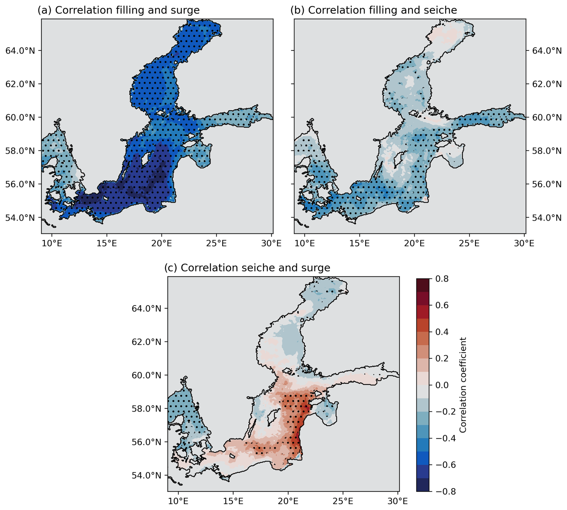
Figure 4 Correlation maps for the three temporal components. (a) Correlation coefficient for the surge and filling components. (b) Correlation coefficient for the filling and seiche components. (c) Correlation coefficient for the seiche and surge components. The hashed areas indicate where the p value is below 0.05.

Although located outside the semi-enclosed Baltic Sea, stations in the Kattegat and Skagerrak (stations 20–28) and in the North Sea (station 72) still exhibit large filling contributions of 40 %–50 %. This shows that, at least for ESL events, low-frequency waves such as the filling contribute to the slow sea level variability. This makes sense, as the mean filling of the Baltic Sea is controlled by the water exchange with the North Sea, which requires long periods of elevated sea level in front of the Danish Straits. Since tides are excluded in the simulations, the low-frequency variability cannot be a superposition effect such as the spring–neap cycle, further indicating that low-frequency waves also contribute significantly to ESLs in the more open eastern North Sea. As a contrast to the Baltic Sea stations, we included one station in the North Sea, Cuxhaven (71). The model deviates from the observations for this station in the southeastern North Sea because tides are not included in the model. Nevertheless, the filling contribution to the ESLs of about 25 % is a noteworthy result, indicating that persistent westerlies can elevate the mean sea level for a period of at least 1 week or longer in this region.

3.1.1 Correlations between the components

A correlation analysis (Pearson's correlation coefficient) of the three temporal components (Fig. 4a–c) reveals that the filling and the surge components are negatively correlated for the western and central Baltic Sea (Fig. 4a). The filling and the seiche components show only a weak negative correlation (Fig. 4b). The seiche and surge components are positively correlated for the central and eastern Baltic Sea (Fig. 4c).

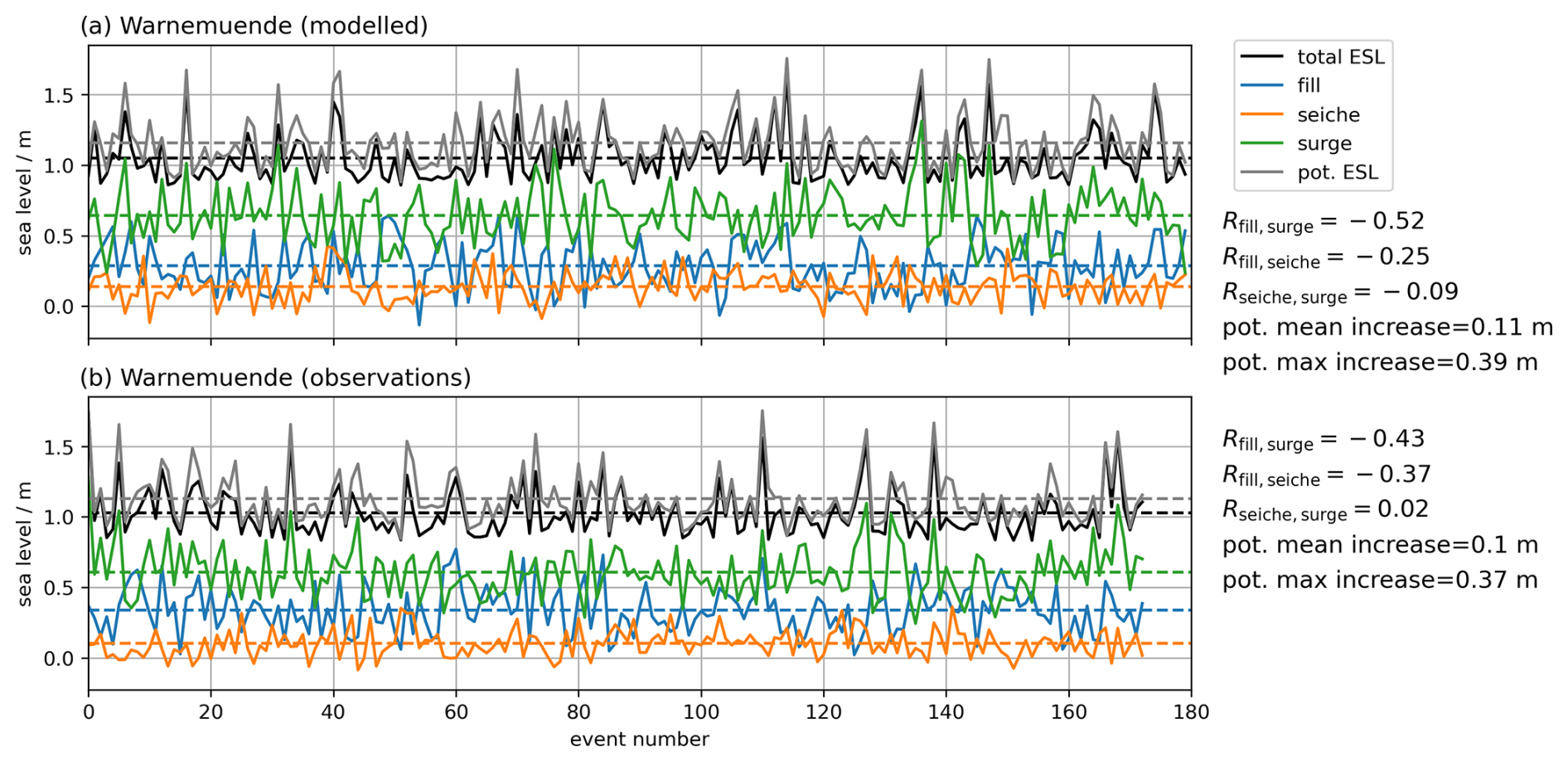
Figure 5 Illustration of the temporal decomposition and the correlation between the components for the Warnemünde station. (a) The three components of filling, surge, and seiche for the ESL event modelled. (b) As (a) but using the observed ESL events. The maximum ESL heights are shown in grey, e.g. the potential sea level if the surge peak, the seiche peak, and the maximum filling (all ± 24 h around the surge peak) co-occurred.

The negative correlation between surge and filling is surprising at first sight, as it is known that most ESLs in the Baltic Sea are a combination of both contributions. At second glance, it does not contradict the fact that most ESLs are a combination of high filling states and storm surges, which would intuitively indicate a positive correlation. The negative correlation between the relative filling and surge components is partly an artefact of the decomposition method since we do not correlate the whole time series but only the extracted statistical samples that we used for the Gaussian distribution fits. Since the peak sea level of each event is fixed, a particularly high surge (the right side of the surge's Gaussian distribution) must naturally coincide with a lower filling state relative to the mean of the Gaussian distribution (the left side of the filling's Gaussian distribution), which emphasizes a negative correlation. Otherwise, the average relative ESL would be higher than 100 %, and thus the fitted Gaussian distributions would be wrong. The same applies to a low surge and a high filling state. Therefore, these two components must be negatively correlated in this decomposition approach of the mean ESL. For the Warnemünde station, this negative correlation is clearly visible, for both the modelled and the observed ESL events (Fig. 5, here with non-normalized sea levels). Of course, events where both the filling and the surge components are very high relative to their mean are also possible and have been observed (Groll et al., 2024). For example, some of the highest peaks at Warnemünde, exceeding 1.5 m (Fig. 5b, event numbers 33, 52, 73, and 110) are formed by the combination of the components of very high surge and high filling. However, the probability of occurrence of ESL events with combined extremely high filling and surge is low. Nonetheless, these events are often among the most devastating ones and can lead to dangerous inundations in the coastal regions, e.g. the historic 1872 surge (Hofstede and Hamann, 2022).

The positive correlation between the seiche and the surge can be explained by the initialization of the seiche by preceding weather systems before the actual surge occurs; i.e. seiches are excited by a previous surge. The stronger the subsequent system, the higher the seiches initialized by the previous system are likely to be. It is also likely that the frequency of the seiches is comparable to the duration of the surges, so the forced fit may overestimate the height of the seiches during the ESL event. Areas where the correlation is low and not significant indicate that the phase of the seiche during the surge's peak is random.

The negative correlation between filling and seiches shows smaller coefficients than between the filling and surge components, indicating that seiches tend to be small when filling is high and vice versa. Since there is a positive correlation between surges and seiches and a negative correlation between filling and surges in the same areas, it makes sense that seiches would generally be negatively correlated with filling as well.

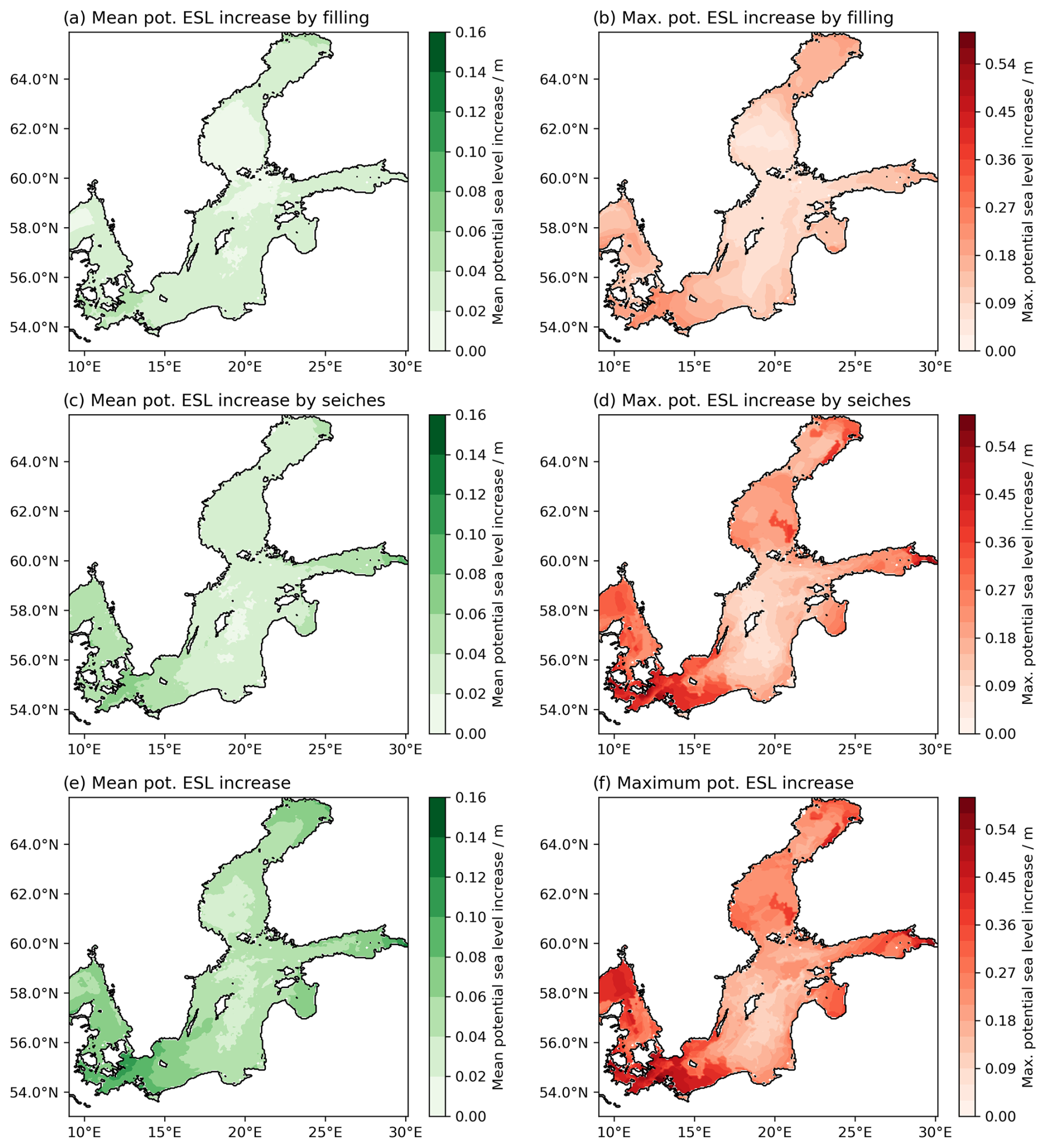
Figure 6 Potential increases in the ESL event if the three temporal components were compounding, e.g. if their maxima occurred simultaneously. (a) Mean potential increase from the filling component (difference in maximum filling around the ESL peak (± 24 h) to the actual filling at the ESL event). (b) Maximum increase in the filling component. (c) As (a) but for the seiche component. (d) As (b) but for the seiche component. (e) Potential mean sea level increase if the surge peak, the seiche peak, and the maximum filling occurred at the same time (sum of a and c). (f) As (e) but for the maximum ESL increase within all ESL events in the respective grid cell (sum of b and d).

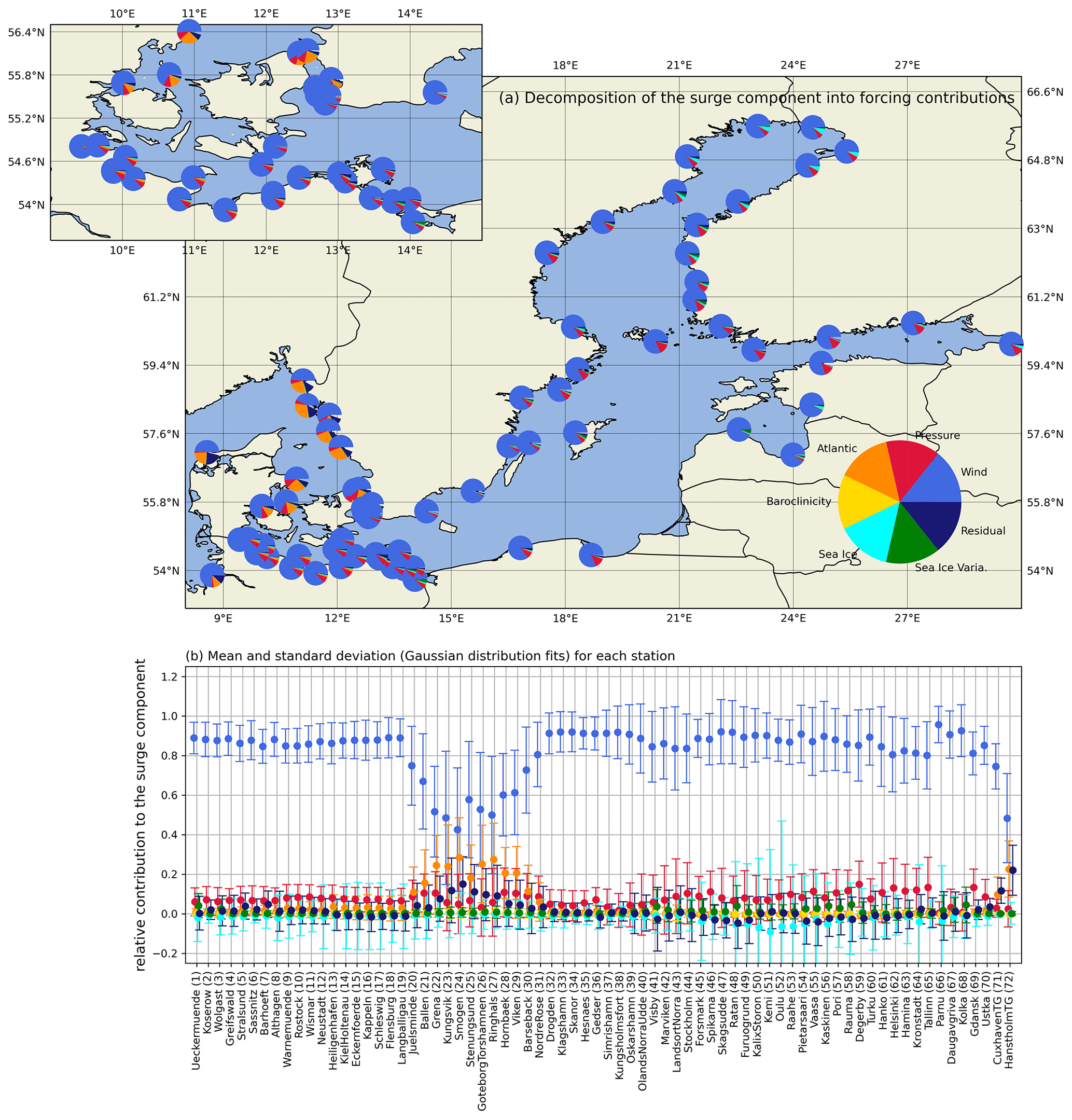
Figure 7 Decomposition of the surge component into forcing contributions. (a) Pie charts of the relative forcing contribution of each station scattered over the Baltic Sea. (b) Relative contributions regarding the mean and standard deviation (based on Gaussian fits) for each station. Note that the pie chart depiction only considers the absolute values and not the sign.

3.1.2 Potential increases in maximum sea levels by time shifting the components

Since the low-frequency waves of the filling component and the high-frequency contributions from seiches and surges operate on different timescales, the timing of their peaks should be independent of the filling levels, essentially making them random. Therefore, we assess the potential increase in peak sea levels under a worst-case scenario, where the peaks of all three components align. Specifically, we examine the maximum filling levels and seiche heights within a 48 h window surrounding the ESL peaks. For the Warnemünde station, the mean and maximum potential increases due to these compounding components are 11 (10) cm and 39 (37) cm, respectively, where the values in the brackets are from the observations (grey in Fig. 5). A more detailed examination of these potential increases shows that the filling component has less potential to increase the ESLs than the seiche component (Fig. 6a–d). On average, the filling could have increased the ESLs by only a few centimetres (Fig. 6a), whereas the maximum increase could have been in the range of 10–20 cm (Fig. 6b). If the seiche peaks were aligned with the surge peaks, the mean increase could reach 10 cm (Fig. 6c) and the maximum increase up to 30–40 cm (Fig. 6d). The largest mean increases are found in the western Baltic Sea and at the head of the Gulf of Finland, with values between 10 and 15 cm (Fig. 6e). The largest maximum increases are also found in these regions, with values reaching up to 50 cm (Fig. 6f). The large potential increases in the northern Baltic Sea most likely correspond to the effect of seiches introduced by the preceding storms, i.e. the clustering of passing storm systems as described by Rantanen et al. (2024). The potential increases by seiches are small in the central Baltic Sea, where a positive correlation between the surge and the seiches is found (Fig. 4c).

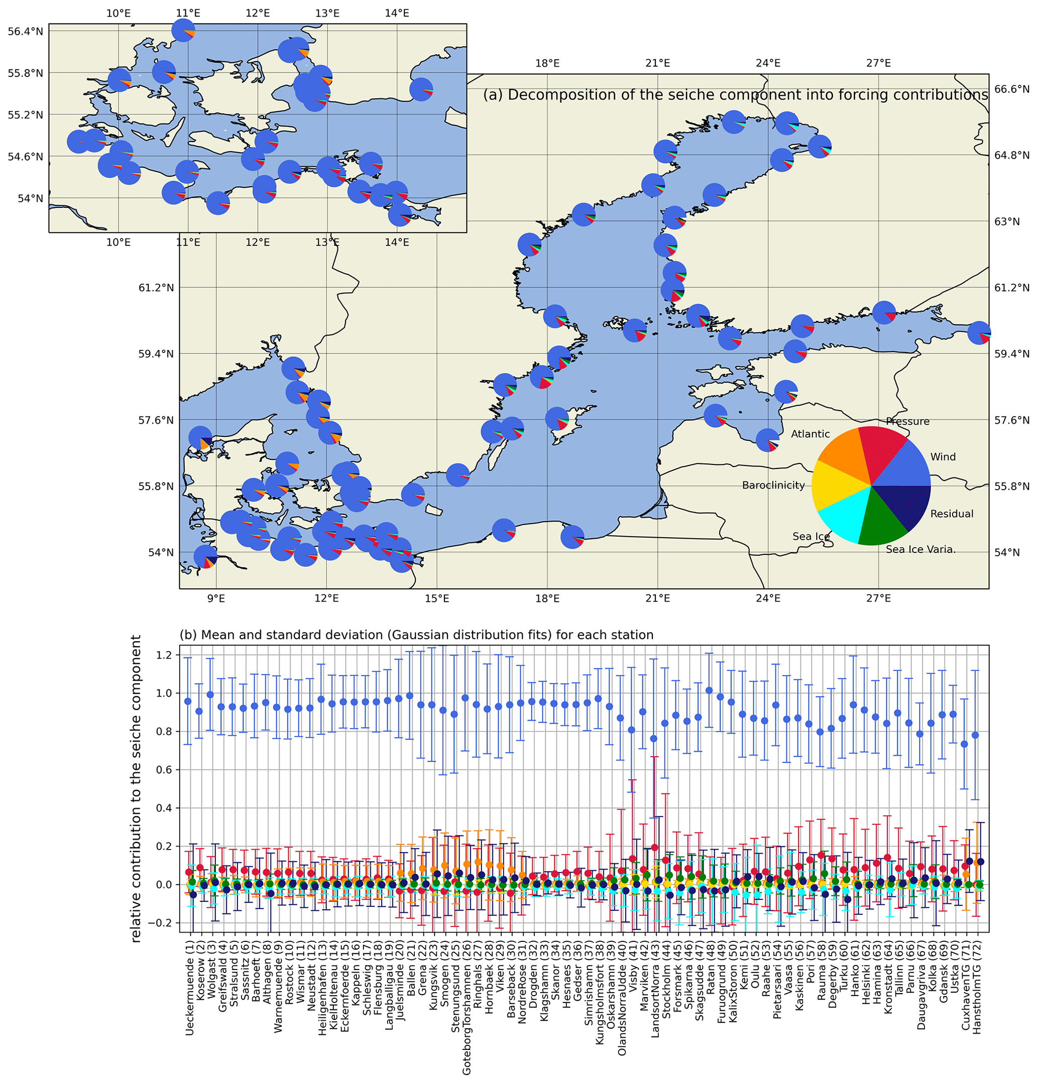
Figure 8 Decomposition of the seiche component into forcing contributions. (a) Pie charts of the relative forcing contribution of each station scattered around the Baltic Sea. (b) Relative contributions regarding the mean and standard deviation (based on Gaussian fits) for each station. Note that the pie chart depiction only considers the absolute values and not the sign.

3.2 Decomposition into forcing components

As expected, the surge component is almost entirely explained by the winds. Throughout the Baltic Sea, winds account for 80 % or more of the surge heights (Fig. 7). The remainder is mainly explained by atmospheric pressure. Winds continue to be the most important surge forcing for the Kattegat, north of the Danish Straits, and outside the Baltic Sea basin. However, the Atlantic sea level component can contribute up to 30 % of the surge levels for this region. This indicates that some of the surges in this region originate outside the model domain. Their fetch lengths exceed the distance from the Kattegat/Skagerrak to the open boundary. Therefore, these surges are introduced by the boundary conditions of the northwestern Atlantic through the inverse barometric effect. The winds within the model domain then amplify these surges. The effect of sea ice is limited to the Gulf of Bothnia and the head of the Gulf of Finland, where the surge height can be reduced by 10 % on average and even more for individual events, which is on the order of the expected magnitude (Zhang and Leppäranta, 1995).

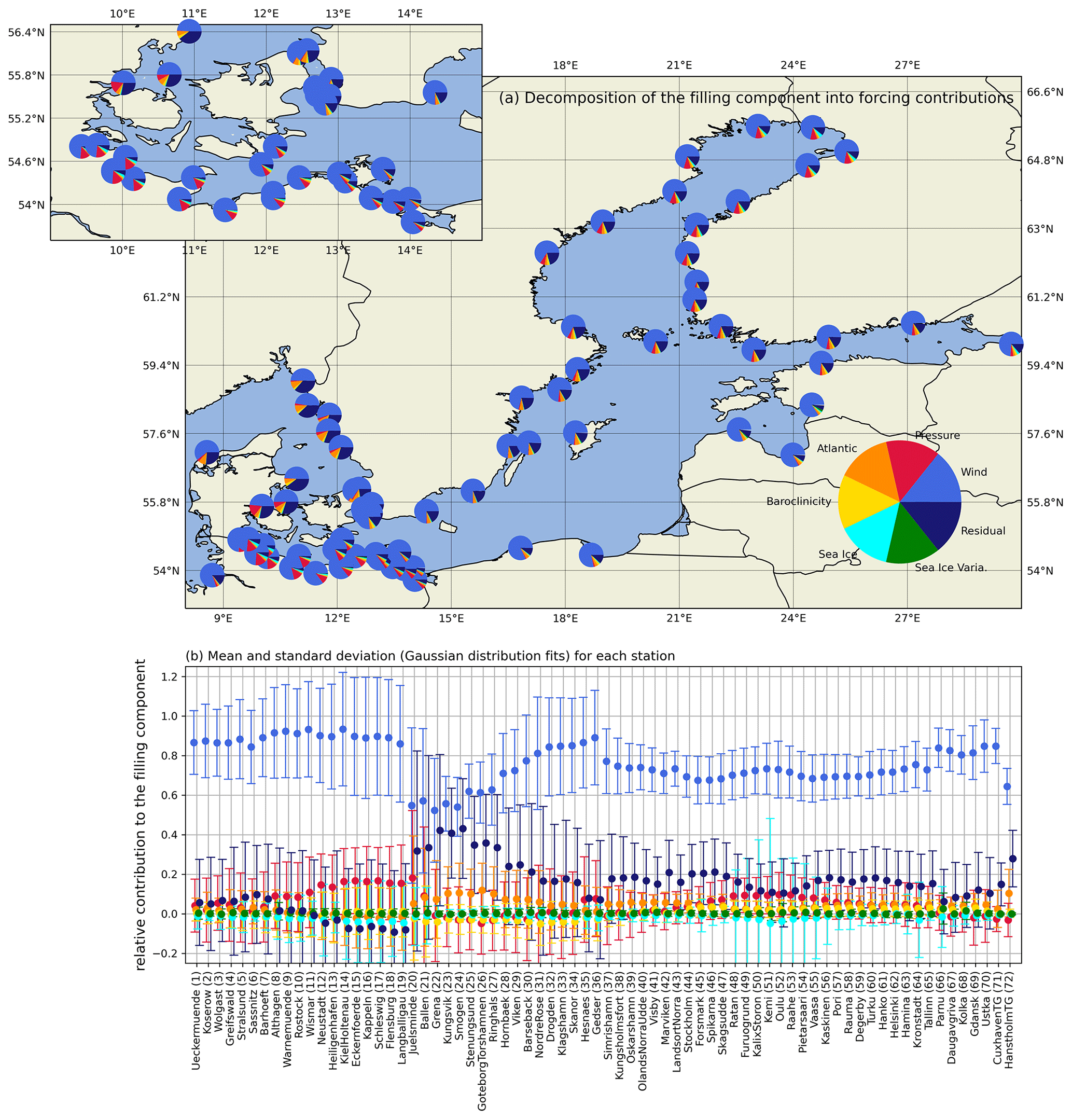
Figure 9 Decomposition of the filling component into forcing contributions. (a) Pie charts of the relative forcing contribution of each station scattered around the Baltic Sea. (b) Relative contributions regarding the mean and standard deviation (based on Gaussian fits) for each station. Note that the pie chart depiction only considers the absolute values and not the sign.

Similarly, winds account for the seiche component almost everywhere, with minor contributions from atmospheric pressure in the Baltic Sea (Fig. 8). The Atlantic component also plays a role in the Kattegat near the Danish Straits. Generally, the fitted seiche periods are based on the seiche frequencies in the Baltic Sea basin. Therefore, the seiche frequencies chosen likely do not correspond to the actual seiches for this region. This discrepancy may explain why the seiche component in the Kattegat and Skagerrak is the smallest contributor to the ESLs. Furthermore, sea ice has a minor influence on the seiches in the Gulf of Bothnia.

The filling component is also mainly determined by the wind forcing (Fig. 9), with contributions ranging from 50 % in the Kattegat and Skagerrak to more than 80 % in the western Baltic. For the western Baltic Sea, atmospheric pressure is the second-largest contributor to the filling component. The other forcings contribute a few percent to the mean filling for the rest of the Baltic Sea basin. In contrast to the surge and the seiche components, the residual term shows values of up to 20 % within the Baltic Sea. The wind and Atlantic sea level forcings explain most of the filling for the Skagerrak and Kattegat. However, the residual term shows values up to 40 % across these regions. These large residuals indicate that the assumed linearity of the decomposition into forcings does not hold well for the filling component, likely due to temporal shifts in low-frequency waves.

The results of the forcing decomposition show that the inter-annual variability in sea ice has a negligible effect on ESLs due to its minimal contribution to any of the three temporal components: surge, seiche, or filling (Figs. 7–9). The inter-annual variability in the baroclinicity of seawater has no effect on the high-frequency surge and seiche components (Figs. 7 and 8) and only a minimal effect on the filling component. The Atlantic sea level mainly affects the surge component for the Kattegat and Skagerrak, while its contribution to the filling component is limited to a few percent. As expected, the wind and air pressure forcings are the main forcings for all three components, with the wind being the most important.

4 Discussion

4.1 Components

4.1.1 Importance of the components and forcings

Our results show two distinct temporal compositions of the ESLs: in the western Baltic Sea, the primary component is the surge, which acts upon the local filling state and is modulated by the seiche component. In contrast, filling is the primary driver in the rest of the Baltic Sea basin, with relatively smaller surges acting on top. Again, the seiches modulate the peak sea level. For the Kattegat and Skagerrak outside the semi-enclosed basin, the contributions of filling and surge are almost equal, with the seiche being the component contributing the least. Different primary contributors can lead to variations in the characteristics of ESLs, potentially causing differences in their dynamics, persistence, and probability of occurrence at specific locations.

This distribution of two distinct contributors to ESLs corresponds to the dominant wind climatology in the Baltic Sea region. Westerly winds generate high filling (Gräwe et al., 2019) and often cause storm surges on the west-facing coasts of the Baltic Sea. There, the filling is the main contributor, and surges also play a significant role. The east-facing coasts of the Baltic Sea are sheltered from these prevailing winds, so the filling component is the most influential factor there, with the exception of the western Baltic Sea. While strong winds from the north and east are less frequent (Soomere and Keevallik, 2001), these winds cause surges along the coasts of Germany, Denmark, and Sweden.

Although the importance of the filling component has been recognized in the literature before (e.g. Soomere and Pindsoo, 2016; Pindsoo and Soomere, 2020), this study provides quantitative figures that underline its significance. For the western Baltic Sea, the mean contribution of filling is less than the contribution of surge, which is consistent with the recent results of Groll et al. (2024), who studied the contributions of surge and filling in the western Baltic Sea. This is partly because water can flow into the Kattegat, Skagerrak, and North Sea on the timescale of the filling, which is about a week. Nevertheless, it is a fact that both filling and surge compounded during the highest-ESL events that caused severe historical inundation and damage, e.g. in 1872 (Hofstede and Hamann, 2022) or 2005 (Suursaar and Sooäär, 2007; Mäll et al., 2017).

We have demonstrated that temporal shifts towards simultaneous alignment of the maximum sea levels of the three temporal components can increase the ESLs by several decimetres within each event. It has to be noted that the force-fitting approach can lead to a positive bias of potential increases, especially if the surge duration is similar to one or more of the seiche periods. Therefore, the maximum potential increase due to the seiches (Fig. 6d) and hence the maximum total increases (Fig. 6f) are most likely overestimated. Nevertheless, the potential average increase due to temporal shifts in the seiche and filling is on the order of 10–20 cm. These values represent the theoretical maxima of ESLs in the respective regions for the specific events.

Our analysis of the forcing contribution clearly shows that wind and air pressure are by far the most important contributors to the ESLs in the Baltic Sea region.

Sea ice is known to reduce the local momentum transfer to the water and therefore reduce storm surges (see Zhang and Leppäranta, 1995, for the Baltic Sea). For the northern Baltic Sea, sea ice is present every winter during the storm season, which we have included in our simulations. Our model simulations suggest that sea ice reduces the surge component by 10 % on average, translating into sea level changes in the range of decimetres, as shown by Zhang and Leppäranta (1995). In regions where sea ice is present in winter, the filling component is the main contributor to ESLs, which is almost unaffected by sea ice, as filling is a basin-wide process. However, with decreasing levels of sea ice due to climate change (e.g. Meier et al., 2022a, b, and references therein), the contribution of storm surge to ESLs is likely to increase in the future in regions that are currently covered by annual sea ice. The same argument can be made for the inter-annual variability in sea ice. Our results show that this contribution to the ESLs is currently very small (Figs. 7–9). However, in a warming climate, the contribution of inter-annual variability to sea ice may increase.

The inter-annual effects of baroclinic density fields on ESLs are found to be negligible, indicating that baroclinic contributions to water transport are not important for ESL events in the Baltic Sea.

4.1.2 Excluded components and forcings

Many coastal regions of the world have tidal regimes that allow ESLs to occur only during high tide and also interact with storm surges (Arns et al., 2020). In the Baltic Sea, the tides are generally very small (< 10 cm) and confined to the western Baltic Sea (e.g. Gräwe and Burchard, 2012). Therefore, we expect tide–surge interactions to be small (Arns et al., 2020). Their mean relative contribution to ESL events should be zero, as the occurrence of the surge should be uniformly distributed over the tidal cycle. Consequently, we have deliberately excluded the tidal component from our temporal decomposition. For tidal regions, it can easily be added to the decomposition.

For the decomposition into forcings, we have also omitted the process of wave setup, e.g. momentum deposition due to breaking surface wind waves, which can also contribute to ESLs (Longuet-Higgins and Stewart, 1964). In the eastern Baltic Sea in the Gulf of Finland, wave setup can contribute several decimetres to ESLs in some coastal segments, resulting in relative contributions of up to 50 % (e.g. Soomere et al., 2013). It should be noted, however, that these estimates are subject to large uncertainties due to assumptions made about the relationship between the offshore wave heights and the wave setup itself. In the western Baltic Sea, the effect of wave setup on ESLs is only a few centimetres (Su et al., 2024). However, the potential contribution of wave setup can be substantial in specific locations, e.g. for exposed coasts of islands (Su et al., 2024) or coastal bays (Soomere et al., 2013). The challenge in accurately assessing the wave setup component lies in the need for high-resolution data on wind wave properties within the surf zone, which even state-of-the-art hydrodynamic models struggle to capture on large scales, such as the entire Baltic Sea. Running a wave model with such a fine resolution at this scale is not feasible. As a result, distinguishing wave setup from the direct momentum transfer caused by wind remains a task for future research.

In general, the exclusion of wave setup should not affect our results much, as the model can reproduce the ESL statistics (Lorenz and Gräwe, 2023a) and the temporal decomposition of the observations (Fig. 3). Thus, the transfer of momentum from the atmosphere to the ocean via the transfer bulk formula is able to reproduce the ESLs. However, it should be noted that the wind speeds were increased by 7 %, which was necessary to match the ESLs with the observations, especially in the western Baltic Sea (see Lorenz and Gräwe, 2023a, for a discussion of this issue). This increase may partly compensate for the missing wave setup. Nevertheless, this would not diminish the relative importance of the wind forcing. It would only split the wind component into a direct sea level component, the generation of long surface waves, and an indirect sea level input via the breaking of surface wind waves within the surf zones.

Similar to the wave setup, we have excluded meteotsunamis (Monserrat et al., 2006; Pattiaratchi and Wijeratne, 2015b). These are tsunami-like surface waves generated by the matching of the propagation speeds of a small atmospheric pressure jump and the induced surface wave, e.g. Proudman resonance (Proudman, 1929). The reasons for neglecting meteotsunamis are simple: first, the temporal and spatial resolution of the meteorological forcing is too coarse to resolve the propagating pressure system accurately enough to generate meteotsunamis in the numerical model. Second, the hourly resolution of the observational data used is also too coarse to resolve the meteotsunamis that occur on faster timescales (minutes). Nevertheless, meteotsunamis could occur during an ESL event (Pattiaratchi and Wijeratne, 2015a) and are a common phenomenon in the Baltic Sea (Pellikka et al., 2020, 2022), with high sea level contributions on the order of decimetres. Meteotsunamis could easily be included in the temporal decomposition using a high-pass filter.

We have also ignored the influence of river discharge since the coarse resolution of our model does not sufficiently resolve the estuaries and constrictions where river discharge increases sea level. However, compounding ESLs with very high river discharge can elevate the peak sea level (Talke et al., 2021), and this has been observed in the southwestern Baltic Sea (Heinrich et al., 2023). We do not expect major changes in our results, as these effects are restricted to estuaries, and we have studied ESLs at the open coast. Nevertheless, we acknowledge the importance of river discharge in estimating coastal flooding.

4.1.3 The residual term and non-linear interactions

In decomposing the different forcing components, a residual term has been added to the right-hand side of Eq. (4) to account for non-linear effects between the forcing contributions and unaccounted forcings. The residual term is not important for the seiche component. However, for individual events, the assumption of linear superposition may not hold since the standard deviation of the residual term is in the range of 10 %–20 %. For the surge component, the decomposition into forcings works well. Both the mean residual and the standard deviation remain small, except for in the Kattegat region. There, the residual term becomes notably large, indicating the presence of non-linear interactions. These interactions could affect both the sea level height and the timing, leading to temporal shifts. Similarly, the residual term for the filling component is non-zero throughout the Baltic Sea. Overall, the residual term is not negligible for any temporal component, clearly showing the interactions between the different forcings on the simulated sea levels. Nevertheless, our results quantify the importance of the different forcings relative to each other, which should be independent of the residual term.

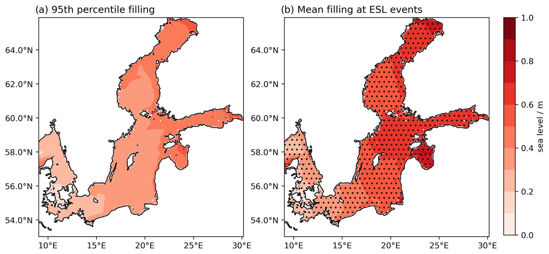
Figure 10 Comparison of (a) the 95th percentile of the filling component to (b) the mean filling component during the ESL events. The hashed area indicates where the mean filling during the ESL events is higher than the 95th percentile in (a).

The temporal decomposition performed in this study (Eq. 1) does not allow the quantification of non-linear interactions between the different timescales. Although these non-linear interactions are included in the respective time series, the computation of the three components automatically attributes all non-linear interactions to the surge component (see Eq. 3). However, the non-linear interactions between the temporal contributors are expected to be small in the Baltic Sea (Arns et al., 2020).

4.2 Consequences for ESL statistics

The results indicate that the following three temporal components are correlated: a negative correlation between filling and surge, a weak negative correlation between filling and seiche, and a positive correlation between the surge and seiche. This suggests that the contributors are not independent, which has implications for classically applied ESL statistics. The observed negative correlation between components hints that return levels based on classical ESL statistics may be overestimated. However, it is important to emphasize that these negative correlations are based on the statistics of all values exceeding the 99.7th percentile. Furthermore, as we have already described, the negative correlation can be an artefact of the decomposition approach (Sect. 3.1.1). It is commonly assumed that the ESL distributions can be described by either the generalized extreme value (GEV) distribution or the generalized Pareto distribution (GPD; Coles, 2001). However, as, for example, Suursaar and Sooäär (2007) note, some outliers do not fit these distributions. Kudryavtseva et al. (2021) suggest that these outliers could be caused by a sequence of storms that initially increases the filling state of the Baltic Sea and then creates a surge on top of it. Our results show that, on average, the opposite is the case, making these outliers stand out even more. Historical ESL events, such as the 2005 (Suursaar and Sooäär, 2007; Mäll et al., 2017) or the 1872 surge (e.g. Hofstede and Hamann, 2022; Andrée et al., 2023), were a superposition of extremely high filling (71 cm at Landsort and up to 100 cm in the western Baltic Sea for 1872 and > 70 cm for 2005) and an exceptional surge. MacPherson et al. (2023) argue for the inclusion of these historical events, as they substantially influence (increase) the sea level design. This is particularly important for the western Baltic Sea, where the ESL activity has been relatively low over the last 70 years, which is the basis for current ESL statistics and design levels (MacPherson et al., 2023).

Note that none of the statistical approaches mentioned have considered the temporal decomposition of the low- and high-frequency contributions or the interdependence between different components. If the statistics of two (or more) components were considered independently, the peak sea level resulting from the summation of the sea levels of the components with the same return period (the same probability) would be overestimated because correlations between the components are neglected. Comparing the 95th percentile of the filling component with the mean filling during the ESL events considered in this study (Fig. 10) highlights a key point: the mean filling during ESL events consistently exceeds this percentile threshold across the entire Baltic Sea. This demonstrates a clear coupling between high filling levels and surges, suggesting that a combined statistical distribution, as is traditionally used, remains preferable. However, as discussed in the previous paragraph, this approach may not accurately reflect historical events.

Incorporating the correlations between the three temporal components using copula statistics could enhance the statistical representation of ESLs in the Baltic Sea. This method may help to reduce uncertainties in the tail ends of ESL distributions, which are a major source of error when determining design levels for coastal protection. To the best of our knowledge, this approach has not yet been applied to ESLs in the Baltic Sea region.

4.3 Consequences for numerical modelling and climate projections

The clear and dominant importance of winds for the generation of ESLs in the Baltic Sea is expected from physics but poses a problem for numerical ocean models. Since the uncertainty in the storm systems in the atmospheric data is related to the uncertainties in the representation of ESLs in the ocean models (Lorenz and Gräwe, 2023a), the models depend on good atmospheric data.

This poses a significant challenge when estimating how ESLs will respond to climate change in the region. Hindcast simulations demonstrate wide variation in ESL statistics, even when using an ensemble approach (Lorenz and Gräwe, 2023a). The uncertainty is further compounded by the unpredictable evolution of storm tracks and storm intensities, making future projection even more uncertain (see the recent Baltic Earth Assessment Reports and references therein, e.g. Meier et al., 2022a, b; Rutgersson et al., 2022; Weisse et al., 2021). Therefore, the current state of knowledge is that the storm statistics will most likely stay the same in the future (Meier et al., 2022b) since there has been no robust change in storms in current regional climate models for the Baltic Sea region. However, it is certain that sea ice cover will decrease in the future and the mean sea level will rise (Fox-Kemper et al., 2021; Gräwe et al., 2019). The latter will raise the extreme value statistics to higher baseline levels (Wahl et al., 2017; Hieronymus et al., 2018). For shallow lagoon systems, such as those in the western and southern Baltic Sea, sea level rise will alter water exchange with the Baltic Sea, most likely increasing ESLs there (Lorenz et al., 2023). For the former, increasing ESLs would be expected where sea ice is currently present, e.g. in the Gulf of Bothnia and the Gulf of Finland.

Since future ESL statistics are likely to stay the same, except for higher base levels due to sea level rise and the retreat of sea ice cover, future efforts may be directed towards a better understanding of the current distribution and dynamics of ESLs in the Baltic Sea region. This statement applies to physics, e.g. interactions of the different low- and high-frequency components and their statistical dependencies.

5 Summary and conclusions

We decomposed observed and numerically modelled extreme sea level (ESL) events in the Baltic Sea into three distinct temporal components: the low-frequency filling of the basin (preconditioning), storm surges, and basin-wide inertial oscillations known as seiches. Our findings indicate that the surge component is the dominant contributor in the western Baltic Sea, while the filling component plays the primary role in the central and northern parts of the basin. Although seiches contribute the least, they remain a non-negligible factor.

Through numerical simulations, we further examined the driving forces behind each temporal component. Wind emerged as the primary driver of all components, followed by atmospheric pressure. Atlantic sea levels significantly influence the surge component in the Kattegat and Skagerrak regions, located outside the Baltic Sea. However, the Atlantic sea level primarily affects the filling component within the Baltic Sea. Sea ice was found to impact only the surge component in the northern Baltic Sea, while inter-annual variations in sea ice, salinity, and temperature had no substantial influence on any of the components.

The decomposition framework introduced in this study provides a novel and practical approach to isolate the temporal components and their respective driving forces contributing to ESL events in a non-tidal, semi-enclosed basin like the Baltic Sea. Depending on data availability, this method can be easily adapted to other regions, incorporating additional factors like tides in tidal systems or wave setup. Our framework is valuable for advancing the global understanding of sea level extremes and enhancing coastal risk management strategies.