Assessing the performance and explainability of an avalanche danger forecast model

During winter, public avalanche forecasts provide crucial information for professional decision-makers as well as recreational backcountry users. While avalanche forecasting has traditionally relied exclusively on human expertise, avalanche warning services increasingly integrate data-driven models to support the forecasting process. This study assesses a random-forest classifier trained with weather data and physical snow-cover simulations as input for predicting dry-snow avalanche danger levels during the initial live testing in the winter season of 2020–2021 in Switzerland. The model achieved ∼ 70 % agreement with published danger levels, performing equally well in nowcast and forecast mode. Using model-predicted probabilities, continuous expected danger values were computed, showing a high correlation with the sub-levels as published in the Swiss forecast. The model effectively captured temporal dynamics and variations across different slope aspects and elevations but showed lower performance during periods with persistent weak layers in the snowpack. SHapley Additive exPlanations (SHAP) were employed to make the model's decision process more transparent, reducing its “black-box” nature. Beyond increasing the explainability of model predictions, the model encapsulates 20 years of forecasters' experience in aligning weather and snowpack conditions with danger levels. Therefore, the presented approach and visualization could also be employed as a training tool for new forecasters, highlighting relevant parameters and thresholds. In summary, machine-learning models like the danger-level model, often considered black-box models, can provide reliable, high-resolution, and comparably transparent “second opinions” that complement human forecasters' danger assessments.

1 Introduction

The destructive potential of snow avalanches demands reliable forecasts and timely warnings to ensure safety and mobility in avalanche-prone regions. In Switzerland, snow avalanches are the deadliest natural hazard (Badoux et al., 2016), causing significant economic losses that can exceed several hundred million Swiss francs per year (Bründl et al., 2004). Consequently, the Swiss avalanche warning service issues a daily avalanche bulletin during winter. This forecast provides essential information for the public and local authorities, aiding in decision-making for safe winter backcountry recreation and ensuring public safety on transportation routes and in settlements during periods of high avalanche danger.

Until now, public avalanche forecasting has been entirely a human-expert decision-making process during which avalanche forecasters interpret a wide range of data sources such as weather forecasts, meteorological observations, and snow-cover model outputs, combined with field observations of snow-cover stability and avalanche activity (Techel et al., 2022). In forecast products, the severity of expected avalanche conditions is described with a danger level for a region and specific time period summarizing snowpack stability, its frequency distribution, and avalanche size (Techel et al., 2020a; EAWS, 2021a). Additionally, typical avalanche situations are also communicated using so-called “avalanche problems” (EAWS, 2021b). Despite numerous attempts to employ statistical or machine-learning methods as alternatives to conventional avalanche forecasting (e.g. Schweizer et al., 1994; Schirmer et al., 2009; Pozdnoukhov et al., 2011; Mitterer and Schweizer, 2013), very few of these approaches were successfully integrated into operational avalanche forecasting.

In recent years, the growth in data volumes and advancements in data-driven modelling have opened up new possibilities for developing avalanche-forecasting models. Among them, different machine-learning models have emerged, including models predicting danger levels (Pérez-Guillén et al., 2022a; Fromm and Schönberger, 2022), transferring these predictions to a format similar to human-made forecasts (Maissen et al., 2024; Winkler et al., 2024), identifying typical avalanche problem types (Horton et al., 2020; Reuter et al., 2022), assessing snowpack stability and critical snow layers (Mayer et al., 2022; Herla et al., 2023), or predicting avalanche activity (Dkengne Sielenou et al., 2021; Viallon-Galinier et al., 2023; Hendrick et al., 2023; Mayer et al., 2023). These data-driven approaches can provide relevant and reliable predictions with high spatiotemporal resolution and with a level of accuracy similar to that of human-made forecasts (Techel et al., 2024). Despite rigorous model validation, which is indispensable for models' integration into the forecasting process, the “black-box” nature of many machine-learning models presents an additional challenge to their use. While predictions generated by simpler models can be readily interpreted (Horton et al., 2020; Reuter et al., 2022; Mayer et al., 2023), the “decision-making” behind complex machine-learning models generally remains hidden, making it challenging to understand how variables are weighted to make predictions. Though various methods for explaining machine-learning predictions have been proposed (e.g. Ribeiro et al., 2016; Lundberg and Lee, 2017), so far, these have not been tested for models in an avalanche-forecasting context.

With this study, we have two objectives: to evaluate the performance and to deepen the understanding of the predictions generated by the model developed by Pérez-Guillén et al. (2022a) for predicting avalanche danger levels in Switzerland. To this end, we analysed the live predictions during the initial winter season when the model was tested before avalanche forecasters started to integrate these model predictions into their daily forecasting process. During this forecasting season, the model provided nowcast and 24 h forecast predictions for dry-snow conditions. Here, we compare aspect-specific predictions with danger-level forecasts in the public bulletin, including a comparison of model-predicted probabilities with sub-level qualifiers assigned to danger levels (e.g. Techel et al., 2022; Lucas et al., 2023). Furthermore, we assessed model performance in situations when different avalanche problems were relevant. Finally, to understand the features driving predictions towards a certain danger level and thus to reduce the black-box nature of the model, we employed an explanation model quantifying the impact of the model's input features for each danger level, not only overall but also for individual predictions.

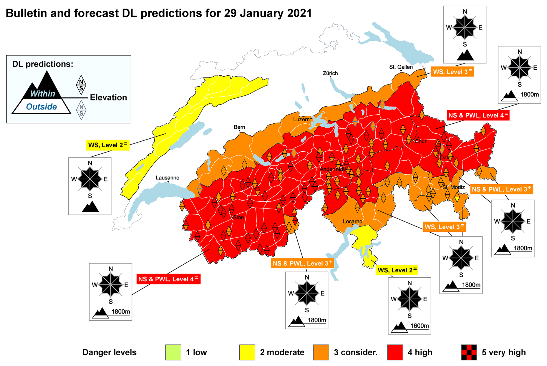
Figure 1 Map of Switzerland showing the forecast danger level (background colour) as published in the bulletin issued on 29 January 2021. In addition, the forecast predictions of the danger-level model are shown for each weather station (represented by triangles). The black contour lines indicate the boundaries of the danger regions, which are aggregates of micro-regions with similar expected avalanche conditions. Critical elevations and slope aspects are graphically indicated on the map, and the main avalanche problem (or problems) is specified (NS: new-snow; WS: wind slab; PWL: persistent-weak-layer), together with the sub-level assigned to the danger level in that region: plus (+), neutral (=), and minus (−). The model predictions are represented by upward triangles for the north (N) aspect and downward triangles for the south (S) aspect, with the colour representing the danger level. Black-contoured triangles denote predictions within the aspects and elevation as specified in the bulletin, whereas grey-contoured triangles represent predictions outside of this aspect–elevation zone.

2 Public avalanche forecast in Switzerland

The avalanche forecast is published at 17:00 LT (local time), valid until 17:00 LT the following day, with an update at 08:00 LT if necessary (SLF, 2023). The forecast domain is split into 149 warning regions (status 2021, average size ≈ 200 km²; white-contoured polygons in Fig. 1), which are clustered into danger regions based on the expected avalanche conditions (black-contoured polygons in Fig. 1). Each danger region is assigned a danger level based on the European Avalanche Danger Scale (EAWS, 2021a; levels: 1-Low, 2-Moderate, 3-Considerable, 4-High, and 5-Very High)¹ summarizing the severity of avalanche conditions. Moreover, the locations of potential avalanche-triggering spots are specified by providing the aspects and elevation where these are most frequent (SLF, 2023). Within the specified aspect–elevation zone, the danger level is applicable (Fig. 1). In addition, the avalanche situation is communicated using the concept of typical avalanche problems (EAWS, 2021b). For dry-snow conditions, three avalanche problems are used (SLF, 2023):

• The new-snow (NS) problem indicates that the current or most recent snowfall can be released.

• The wind slab (WS) problem is given when fresh or recently wind-drifted snow is of concern.

• The persistent-weak-layer (PWL) problem highlights that a persistent weak layer (or persistent weak layers) within the old snowpack are potentially prone to triggering.

In the bulletin, only the avalanche problems that significantly contribute to the danger are mentioned. For dry-snow conditions, at most, two avalanche problems can be specified. If no particular avalanche problem is identified (e.g. at 1-Low), the avalanche situation is reported as no distinct avalanche problem (EAWS, 2021b). During the investigated forecasting season, the published danger level referred to dry-snow conditions in the majority of cases. However, on days when wet-snow problems significantly contributed to the danger – and surpassed the danger level for dry-snow conditions – two separate danger levels corresponding to dry- and wet-snow conditions were issued in the public bulletin. Since the model only accounts for dry-snow conditions, we exclusively used the forecasts issued for dry-snow conditions in this study.

Lastly, since the winter season 2016–2017, forecasters have assigned one of three sub-levels to each danger level, except for 1-Low (Techel et al., 2020b, 2022):

• plus or + means the danger is assessed as high within the level; e.g. a 3⁺ is high within 3-Considerable.

• neutral or = means the danger is assessed as about in the middle of the level; e.g. a 3⁼ is being about in the middle of 3-Considerable.

• minus or − means the danger is assessed as low within the level; e.g. a 3⁻ is low within 3-Considerable.

After 6 years of internal usage, sub-levels have been published in the bulletin since the forecasting season 2022–2023 (Lucas et al., 2023; SLF, 2023). Thus, although the bulletin example for 29 January 2021 shown in Fig. 1 displays this sub-level information, it was not published at the time. When referring to sub-levels, we always mean the combination of danger level with the sub-level modifier.

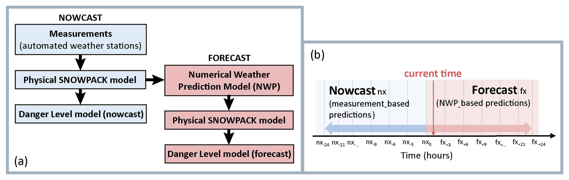
Figure 2 Schematic representation of (a) the steps for running the nowcast and forecast predictions with the danger-level model in the live-testing deployment and (b) the time intervals applied to resample the input features for the model.

3 Danger-level model

Using a 20-year historical data set of snow-cover simulations in Switzerland and information about the avalanche conditions in the region, Pérez-Guillén et al. (2022a) developed two random-forest models to predict the avalanche danger level for dry-snow conditions in Switzerland at the location of more than 100 automated weather stations located mostly above the treeline in the Swiss Alps (indicated by triangles in Fig. 1). One of these models was trained using the forecast danger levels published in the avalanche bulletin as a target variable, while the other used a subset of quality-checked danger levels as labels. The input features for the models comprise a set of meteorological variables, averaged over a 24 h time window similar to the avalanche forecast, and features extracted from the simulated snow-cover profiles (12:00 LT). Table A1 shows the variables used in the operational model. While the predictions of the two models are highly correlated, their danger-level predictions differ sometimes (Pérez-Guillén et al., 2022a). This is caused by the fact that the first model reflects the tendency of the human forecasters to over-forecast (to be on the cautious side), while the second model was trained with a data set reflecting the best hindcast estimate of the danger level. Forecasters opted for live testing the second model. Hence, we exclusively analysed this model in this study.

The model predicts a danger level ranging from 1-Low to 4-High (EAWS, 2021a) since danger level 5-Very High was merged with 4-High when training the model. In our classification setup, the final prediction for a given input x is the average prediction of each tree in the forest:

$$\begin{array}{}\text{(1)}& P\left(D_l\mathrm{|}\mathit{x}\right)={\displaystyle \frac{\mathrm{1}}{T}}\sum _{t=\mathrm{1}}^T{p}_t\left(D_l\mathrm{|}\mathit{x}\right),\end{array}$$

where t is an individual decision tree, T = 1000 is the number of decision trees in the model, D_l where $l\in \mathit{\{}\mathrm{1},\mathrm{\dots },\mathrm{4}\mathit{\}}$ is the danger level on the scale from 1-Low (D₁) to 4-High (D₄), and P(D_l|x) is the mean class probability estimate or confidence score representing the estimated likelihood of belonging to each class (danger level). The sum of the probability estimates across the four classes equals 1. Hence, the final predicted danger level, D(x), is the one showing the highest probability P(D_l|x):

$$\begin{array}{}\text{(2)}& D\left(\mathit{x}\right)=\underset{D_l}{\text{argmax}}P\left(D_l\mathrm{|}\mathit{x}\right),\text{ for }{D}_l\text{ with }l\in \mathit{\{}\mathrm{1},\mathrm{\dots },\mathrm{4}\mathit{\}}.\end{array}$$

Additionally, the expected value, here referred to as the expected danger value, is estimated as the weighted average of all probability scores:

$$\begin{array}{}\text{(3)}& E_D\left(\mathit{x}\right)=\sum _{l=\mathrm{1}}^{\mathrm{4}}\left(P\right(D_l\mathrm{|}\mathit{x})\cdot w_l),\end{array}$$

where $E_D\left(\mathit{x}\right)\in [\mathrm{1},\mathrm{4}]$ is the expected danger value for a given input sample and w₁=1, w₂=2, w₃=3, and w₄=4 for each danger level. Since danger levels are defined on a discrete scale, this value can be interpreted as a numerical value that summarizes the model's prediction on a continuous scale. For instance, if 40 % of the decision trees predict danger level 3 ($P_{D_{\mathrm{3}}}=\mathrm{0.4}$) while 60 % predict a danger level of 4 ($P_{D_{\mathrm{4}}}=\mathrm{0.6}$), the final danger-level prediction is 4-High and the resulting expected danger value is E_D=3.6 but with the added benefit of summarizing the probabilities in a single variable.

Live model deployment

The danger-level model was live-tested for the first time during the winter season of 2020–2021. The model provided real-time nowcast and forecast predictions from the end of December 2020 until May 2021. The nowcast setup followed the following steps (Fig. 2a):

1. Measurements were transmitted every hour from the automatic weather station (AWS) to a server at the WSL Institute for Snow and Avalanche Research SLF.

2. Using these measurements, the snow cover was simulated for flat terrain and for four virtual slope orientations (north: N; east: E; south: S; west: W) with a slope angle of 38° (Morin et al., 2020).

3. The input features required for the model were extracted from the snow-cover simulations every 3 h.

4. Using the extracted input features, the model generated danger-level predictions every 3 h, referred to as nowcast predictions, for each AWS for the flat terrain and the four virtual slope aspects.

In forecast mode (Fig. 2a), snow-cover simulations were initiated using the most recent nowcast simulations (step 2) and were then driven with COSMO-1 numerical weather prediction model (NWP) data as input (COSMO stands for Consortium for Small-scale Modeling; https://www.cosmo-model.org/, last access: 30 March 2025). The NWP data were downscaled to the locations of each AWS according to Mott et al. (2023) to drive snow-cover simulations for the flat study plot and four virtual slope aspects 24 h ahead. In this case, the meteorological input features of the danger-level model were averaged over the next 24 h of the forecast weather time series to forecast danger levels for each AWS and slope aspect. Therefore, for a given time (Fig. 2b), nowcast predictions were computed using features based on averaged measurements from the previous 24 h, while the forecast predictions were based on averaged weather predictions for the next 24 h. For input features computed using historical information of more than 24 h, such as the sum of new snow over 3 and 7 d, the forecast combined the measurements for the upcoming 24 h with nowcast values measured from the AWS.

4 Data and methods

4.1 Test set and model evaluation

For a detailed evaluation of the model's performance, we used the winter season of 2020–2021, during which the model was tested in a live setting for the first time. During this period, only one member of the avalanche warning team (always the same one) reviewed the model's predictions to monitor its performance but not for the operational preparation of the avalanche bulletin. We refrain from analysing later winter seasons, as the model was available to all forecasters from the winter season 2021–2022 onward, potentially impacting the decision-making process and, hence, the forecast product. During the 2020–2021 season, the model provided predictions on 138 d. On these days, the distribution of danger levels for dry-snow conditions in the public bulletin was imbalanced: 21.6 % for 1-Low, 33.8 % for 2-Moderate, 39.1 % for 3-Considerable, 5.3 % for 4-High, and 0.2 % for 5-Very High. To assess the overall performance, we first compared the danger-level predictions by the model at each station with the danger-level forecast in the public bulletin for the corresponding region of the station's location. As the model provides predictions every 3 h, we filtered the predictions starting at 18:00 (local time) and valid for the next 24 h to compare with the bulletin, as this is the time window closest to the avalanche bulletin. In addition, we evaluated model performance by considering both station elevation and virtual slope aspects of the input data compared with the critical elevations and aspects specified in the bulletin (Fig. 1). In this context, we defined the following categories:

• Within the core zone predictions are defined as predictions from stations and virtual aspects that fulfilled both the elevation and the aspect criteria mentioned in the bulletin (represented by black-contoured triangles in Fig. 1). For flat predictions, this meant that only predictions from stations above the critical elevation were included, while aspect-specific predictions were considered only if the respective aspect was considered critical in the bulletin.

• Outside the core zone predictions refer to those below the elevation range specified in the bulletin (see inset in Fig. 1). Predictions for virtual aspects are further categorized into those where only one criterion was not fulfilled (i.e. aspect aligns with the forecast but falls below the indicated elevation) and those where neither condition was met.

During the test period, the forecast for dry-snow conditions in the public bulletin indicated that each aspect was active in the following percentages of cases (considering one forecast per region per day): 99.8 % (N), 97.8 % (E), 64.4 % (S), and 95.7 % (W). The prediction data volumes from the model vary per aspect since the model only generates predictions with the condition of a minimum snow-cover depth of 30 cm (Pérez-Guillén et al., 2022a) and since the simulated snow-cover depth can differ. Therefore, the predictions and forecasts issued within the same forecasting window are individually analysed for each slope aspect by comparing the following (Sect. 5.1 and 5.2):

• nowcast danger-level predictions (D_nx,a) with the forecast predictions (D_fx,a) by the model for each mountain slope aspect (a∈{ F: flat; N: north; E: east; S: south; W: west}),

• forecast predictions (D_fx,a) with the danger-level forecast in the public bulletin (D_bu,a) for each aspect,

• expected danger values computed with the forecast predictions (E_D,a) with sub-levels forecast in the bulletin ($D_{\text{bu},a}^{(-=+)}$) for each aspect.

For the comparison between expected danger values and the sub-levels, we applied a simple rounding strategy: minus rounds to the nearest numerical danger level minus $\frac{\mathrm{1}}{\mathrm{3}}$, neutral rounds to the integer value of the danger level, and plus rounds to $\frac{\mathrm{1}}{\mathrm{3}}$ above the numerical danger level. The same approach was used to convert the danger level–sub-level combination to a numerical value (Techel et al., 2022; Maissen et al., 2024). Additionally, to further investigate the performance of the model across different avalanche problems, we compared the mean agreement rate between model predictions and bulletin for each station with the proportion of days that a specific avalanche problem was forecast in this region (Sect. 5.3). The metrics used to assess model performance are defined in Appendix C.

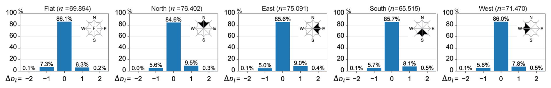
Figure 3 Distribution of the differences between forecast and nowcast predictions ($D_{\text{fx},a}-D_{\text{nx},a}$) for the flat-field aspect and the four virtual aspects ($a\in \mathit{\{}\text{F: flat};\text{N: north};\text{E: east};\text{S: south};\text{W: west}\mathit{\}}$).

4.2 Explainability of model

To understand the predictions of machine-learning models, importance values can be derived for each input feature. There are several ways to explore feature attribution. One of these is SHapley Additive exPlanations (SHAP) (Lundberg and Lee, 2017), an approach based on integrating concepts from game theory with local explanations. SHAP values provide a quantitative method for assigning importance values either locally (for a single prediction) or across the entire data set to explain the model's overall behaviour (Lundberg et al., 2018). To implement this method, we used the Tree SHAP algorithm designed for tree-based machine-learning models, such as random forests (https://shap.readthedocs.io/en/latest/index.html, last access: 30 March 2025). A detailed description of the computation of the SHAP values is shown in Lundberg et al. (2018). This approach uses an additive feature attribution model; i.e. the output is defined as a linear addition of input features. SHAP values measure the contribution of each input feature, which can be positive or negative with regard to the predicted value. SHAP values are bounded by the output magnitude range of the model, which in our case – a random-forest classifier – is from 0 to 1. Therefore, the range of the SHAP values will be from −1 to 1. We applied the SHAP method to obtain global explanations by summarizing the overall importance of features for each class (danger level) of the model (Sect. 6.1), as well as to quantify the contribution of each feature to individual predictions (Sect. 6.2).

5 Results

5.1 Agreement between nowcast and forecast predictions

Overall, forecast and nowcast danger-level predictions correlated well, with Spearman correlation r_s ranging from 0.90 for north to 0.91 for flat (p < 0.01). The corresponding agreement rate varied from 84.6 % (north; Fig. 3) to 86.1 % (flat; Fig. 3). When predictions differed, forecast predictions were slightly more often one danger level higher than nowcast predictions (by 2 %–4 %), except for in the case of flat (Fig. 3). Differences by two danger levels were rare (≤ 0.5 %). Comparing the expected danger values (E_D, Eq. 3) computed with the model-predicted probabilities showed a high correlation between the forecast and nowcast (Pearson correlation r_p of 0.97 ± 0.01, p < 0.01), with a mean difference of 0.0 ± 0.2.

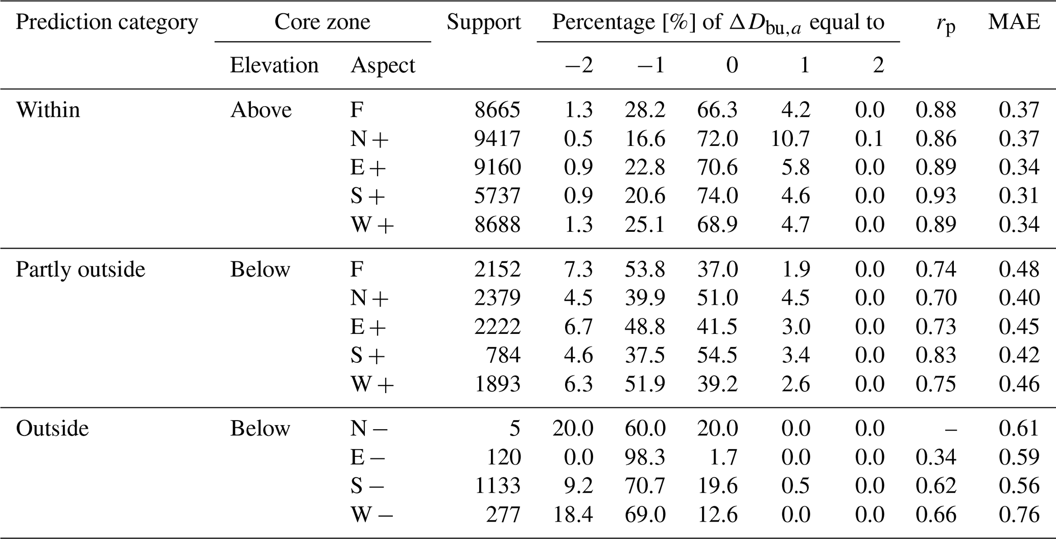
Table 1 Summary of the model's performance during the winter season 2020–2021 based on the forecast predictions: within (elevation: above; aspects ($\text{F: flat};\text{N: north};\text{E: east};\text{S: south};\text{W: west}$): active +), partly outside (elevation: below; aspects: active +), or outside (elevation: below; aspects: non-active −) the core zone ; support of the predictions; and percentage of samples for each forecast model–bulletin bias (ΔD_bu,a, as defined by Eq. C2), which represents the difference between the danger level predicted by the model and the bulletin. Mean absolute errors (MAEs) and the Pearson correlation coefficient are computed using the expected danger values and the sub-level assessments.

5.2 Model agreement with avalanche bulletin

5.2.1 Overall agreement

For stations within the core zone defined in the bulletin (see Sect. 4.1), the mean agreement rate between the danger level published in the bulletin D_bu and the forecast predictions D_fx was 70.4 %, with the lowest agreement rate for the flat-field simulations (66.3 %) and the highest for south aspects (74.0 %; Table 1). South and north predictions generally agreed more with D_bu than flat and other aspects. When D_bu≠D_fx, the differences were mostly by one level, with a larger share of predictions being one level lower (ranging from 20.6 % (N) to 28.2 % (F) in Table 1) rather than higher (ranging from 4.2 % (F) to 10.7 % (N) in Table 1). In comparably few cases (≤ 2.0 %), the difference was by two levels. The agreement rates were lower for predictions that were partly or fully outside the core zone indicated in the bulletin: for instance, for forecast predictions (S), they decreased from 74.0 % within the core zone to 54.5 % when below the indicated elevation but within the aspect range and to 19.6 % when fully outside the core zone (Table 1).

The issued sub-levels ($D_{\text{bu}}^{(-=+)}$; see Sect. 2) correlated strongly with the forecast predictions within the core zone (r_p≥ 0.86, p < 0.01; Table 1). Considering all aspects, the mean absolute error (MAE) was ≤ 0.37 within the core zone (Table 1) but was larger for predictions that were partly or fully outside the core zone (MAE≥ 0.4 and MAE ≥ 0.6, respectively). In other words, predictions partially outside the core zone differed by approximately half a level compared to $D_{\text{bu}}^{(-=+)}$, which increased by about a half to a full danger level fully outside the core zone, reflecting the expected differences in avalanche danger as a function of elevation and aspect (Pérez-Guillén et al., 2022a; Techel et al., 2022). Since similar results were observed for the nowcast predictions (a detailed overview is shown in Table B1), in the following sections, we analyse exclusively the forecast predictions within the core zone.

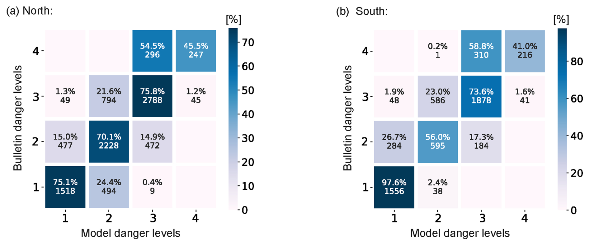
Figure 4 Confusion matrices of the forecast predictions for the aspects (a) north and (b) south. Only predictions from stations within the core zone are considered. The colour map shows the percentage of samples per danger level, calculated row-wise. The numbers below the percentages represent counts.

5.2.2 Level-wise agreement

The diagonals of the confusion matrices shown in Fig. 4 represent the proportion (number) of agreements between the forecast of the model and the bulletin (D_bu; row-wise proportions) for each danger level. These were highest for D_bu 1 to 3. The agreement was generally lower for south than for north aspect predictions, which was most evident for levels 2 and 4. In contrast, south predictions showed considerably higher agreement for D_bu=1 than north predictions. Misclassifications (off-diagonal values in Fig. 4) were typically by one level and rarely by two levels (Tables 1 and B1). The row-wise analysis shows that the model often predicted a lower level than the bulletin, particularly for south predictions and for D_bu=3 in north predictions. Moreover, danger level 2 was the least precise for both aspects, with a higher number of cases where the model predicted danger level 2 while D_bu was equal to 3 (Fig. 4).

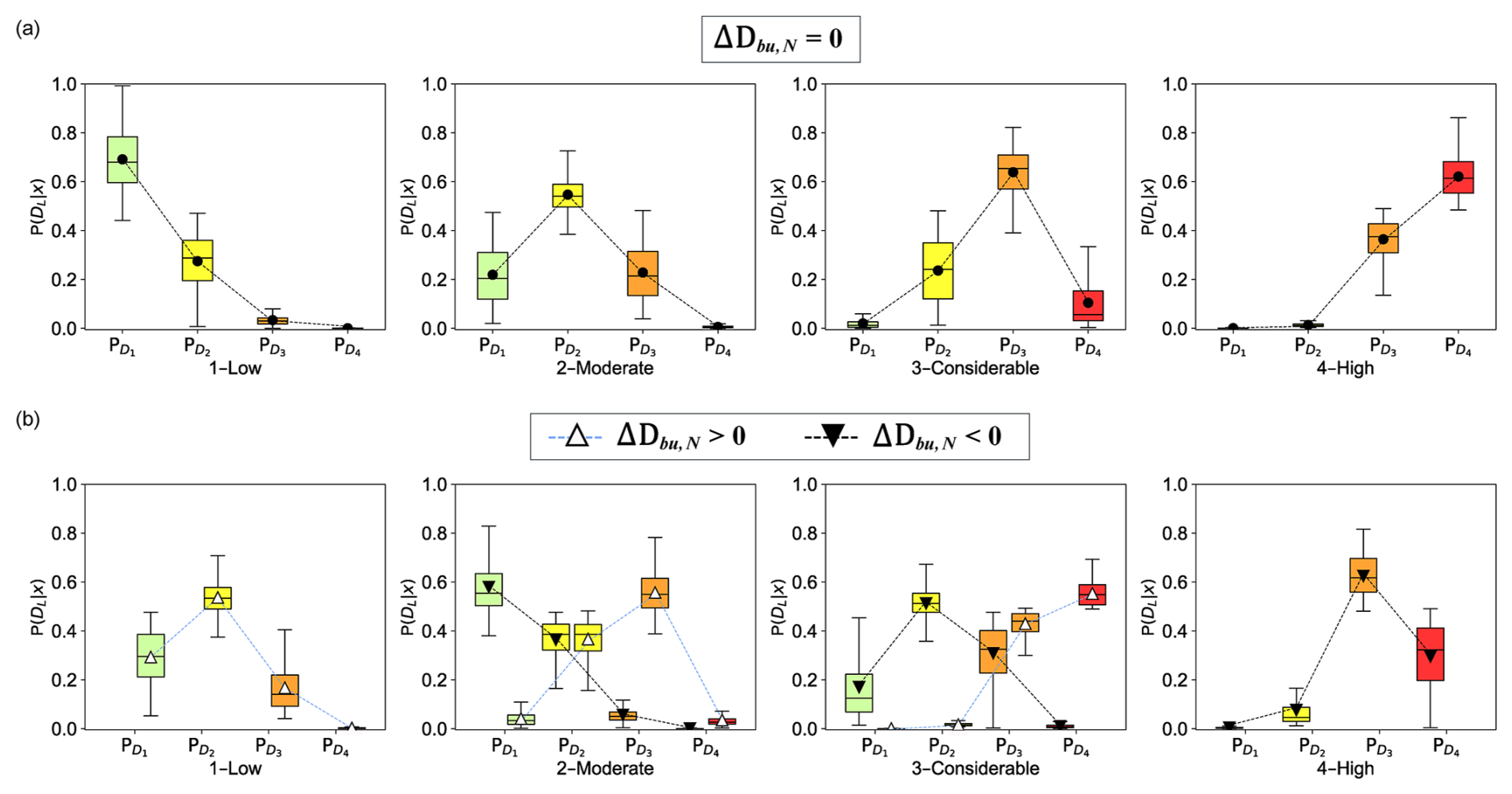
Figure 5 Box plot distributions of the probability outputs from the forecast predictions for each danger-level forecast in the public bulletin split into (a) when the predictions are in agreement with the bulletin ($\mathrm{\Delta }{D}_{\text{bu},N}=\mathrm{0}$) and (b) when they disagree with model predictions higher than the bulletin ($\mathrm{\Delta }{D}_{\text{bu},N}>\mathrm{0}$) or lower ($\mathrm{\Delta }{D}_{\text{bu},N}<\mathrm{0}$). This analysis only considers the within predictions for the north aspect (within–N + predictions of Table 1). The dashed lines link the mean values of the box plot distributions.

5.2.3 Probability estimates

The majority of model predictions were within one danger level of D_bu (Table 1 and Fig. 4). In addition, the distribution of probabilities showed that the model predictions were mainly concentrated between two consecutive levels. Indeed, only a small proportion of the predictions (< 5 %) estimated probabilities > 0.2 for three levels simultaneously and none of them > 0.1 for all four levels.

Comparisons of the probability distributions (forecast mode, north aspect) with the danger level as forecast in the bulletin are displayed in Fig. 5. We distinguish two cases: when the model and the forecast danger level in the bulletin agreed ($\mathrm{\Delta }{D}_{\text{bu},N}=\mathrm{0}$; Fig. 5a) and when they disagreed (Fig. 5b). When predictions matched (Fig. 5a), the mean probabilities ranged between $P_{D_{\mathrm{1}}}=\mathrm{0.69}$ for danger level 1 and $P_{D_{\mathrm{2}}}=\mathrm{0.55}$ for danger level 2. On average, the neighbouring levels had mean probabilities between 0.1 and 0.4. When D_bu was 1 or 4, there were rarely any predictions for two levels higher or lower. When the predictions deviated from the bulletin (Fig. 5b), confidence in predictions decreased, showing higher uncertainty since the mean probability estimates for all danger levels fell below 0.6. Nevertheless, probabilities for the level given in the bulletin were the second highest (between 0.3 and about 0.45); thus, predictions – if different compared to the bulletin – generally tended towards the danger level as forecast in the bulletin.

5.2.4 Sub-level-wise performance

The confusion matrix in Fig. C1 displays the agreement between model-predicted sub-level bins and the bulletin sub-levels. Excluding danger level 1, when no sub-level was assigned, the agreement rate between the forecast sub-levels and the expected danger values was, on average, approximately 30 %, ranging from 0.6 % (4⁼) to 38.3 % (3⁻) (diagonal elements in the matrix of Fig. C1). Deviations from the main diagonal in Fig. C1 were mainly concentrated within one sub-level higher than the bulletin for assessments below 2⁺ and one sub-level lower for assessments below 4⁻. Since the model was trained by merging danger levels 5 and 4, the maximum expected danger values were limited to 4⁼. Thus, the expected values are constrained between the extreme levels of 1 and 4.

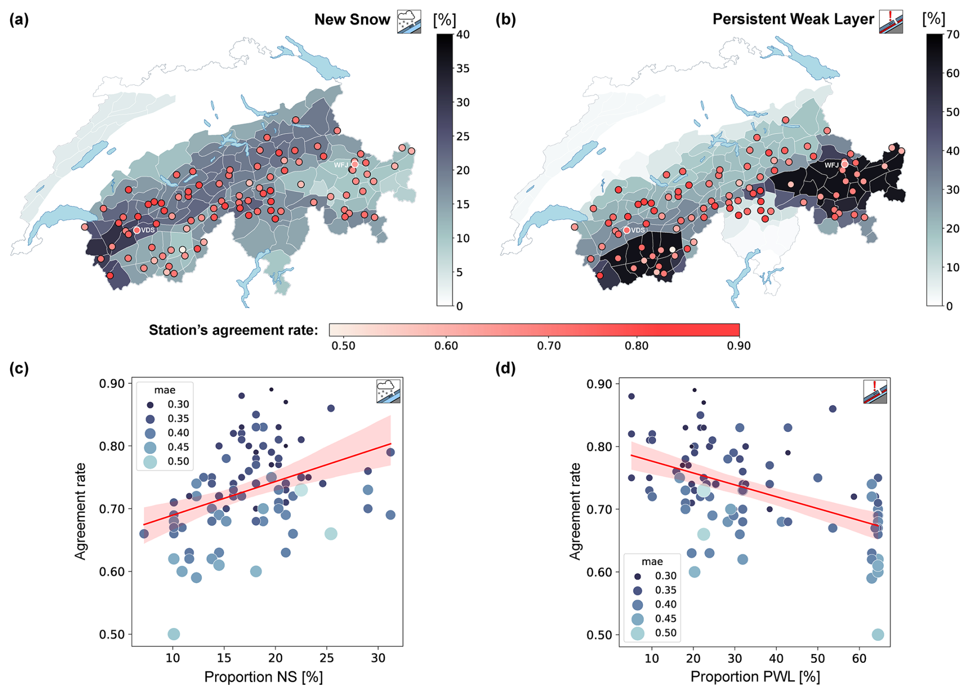
Figure 6 Maps showing the proportion of days regionally forecast in the public bulletin during the winter season 2020–2021 for the new-snow problem (a) and persistent-weak-layer problem (b). Different scales are used for each avalanche problem. The AWSs are coloured based on their average agreement rate calculated using the forecast predictions (N). Only stations with predictions within the core zone on at least 10 % of the days are included. Below, scatter plots show the average agreement rate per station against the proportion of days forecast with new-snow (c) and persistent-weak-layer (d) problems. Linear regression lines and 95 % confidence intervals are marked in red. The dot sizes are coloured and scaled based on the mean absolute error, computed using the expected danger values and the sub-levels forecast in the bulletin.

5.3 Temporal predictions and avalanche problems

As described in Sect. 2, avalanche problems provide information about snowpack characteristics in a region. The map in Fig. 6a shows that the proportion of days with a new-snow (NS) problem exceeded 20 % in the southwestern and central regions of Switzerland, with complementary patterns for the persistent-weak-layer (PWL) problem reaching values of > 40 % in the inner-alpine regions of the Swiss Alps (Fig. 6b). Generally, stations in regions with a frequent PWL problem showed lower mean agreement rates than those in the central and northern regions. Consequently, the correlation between the presence of a new-snow problem and the agreement rate was moderately positive (r_s = 0.42; p < 0.01; Fig. 6c), while it was negative for the presence of a persistent-weak-layer problem (r_s = −0.52; p < 0.01, Fig. 6d). The distribution of the wind slab problem is not shown, as it was forecast for more than 40 % of the days in the Swiss Alps without a clear spatial pattern.

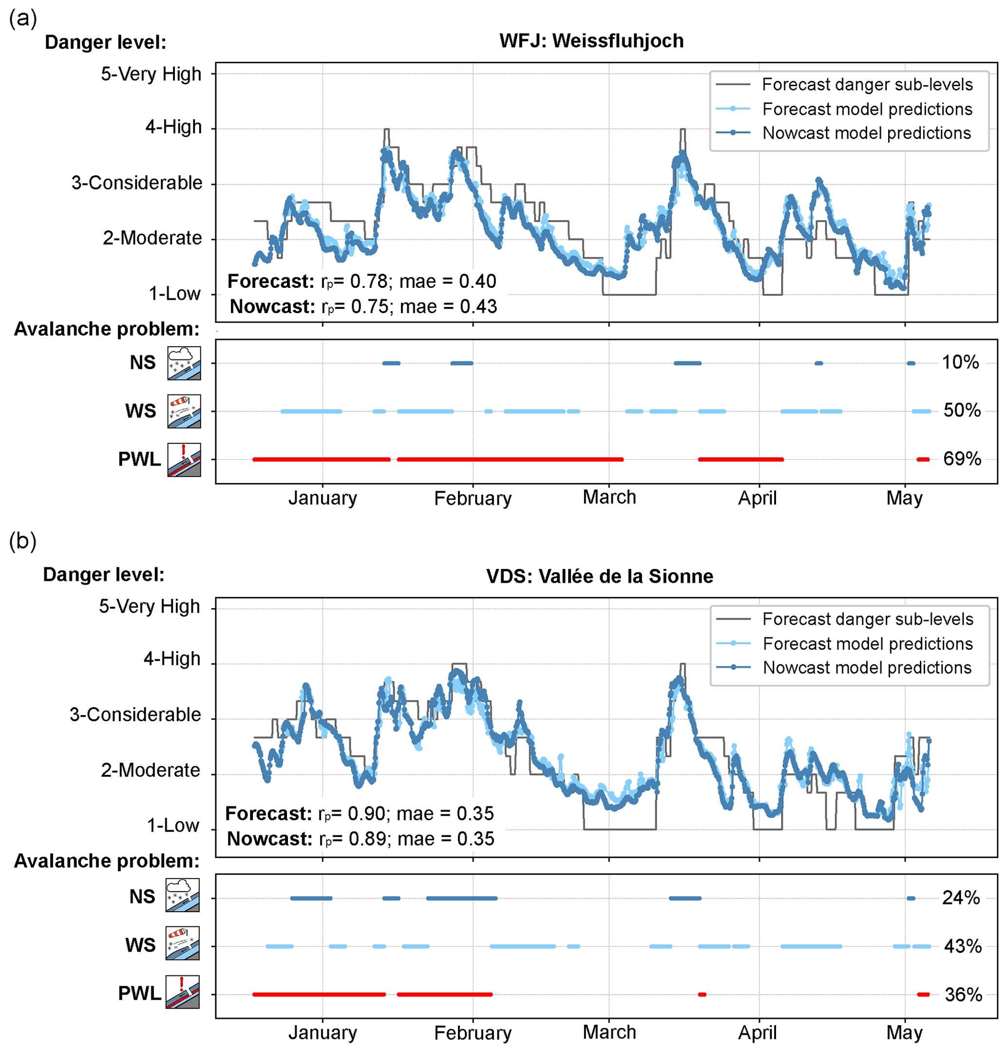
Figure 7 Time series showing the danger level–sub-level combination as forecast in the avalanche bulletin and the model-predicted expected danger values, computed with forecast and nowcast predictions for two automated weather stations: (a) Weissfluhjoch (WFJ; 2536 $\mathrm{m}\mathrm{a}.\mathrm{s}.\mathrm{l}.$) in the eastern Swiss Alps (Fig. 1) and (b) Vallée de la Sionne (VDS; 2385 $\mathrm{m}\mathrm{a}.\mathrm{s}.\mathrm{l}.$) in the western Swiss Alps (Fig. 1). In addition, the avalanche problems for dry-snow conditions as forecast in the bulletin are displayed: new-snow (NS) problem, wind slab (WS) problem, and persistent-weak-layer (PWL) problem.

To evaluate the temporal dynamics of the model predictions across avalanche problems, we selected two stations characterized by different avalanche conditions: Weissfluhjoch (WFJ) located in the Davos region in the east of Switzerland and Vallée de la Sionne (VDS) in the west (locations are shown on the maps in Fig. 6a and b). The main differences between these two regions are related to the frequency of snowfall events and the presence of persistent weak layers within the snowpack. In the region of Davos (Fig. 7a), the NS problem was less frequently forecast compared to in Vallée de la Sionne (10 % vs. 24 % of the days, Fig. 7b) and, conversely, the PWL problem more often (69 % vs. 36 %). Overall, in both regions, model predictions matched the changes in the danger level as forecast in the bulletin, albeit with different time lags depending on the avalanche situation (Fig. 7). The expected danger values correlated well with the forecast sub-levels (WFJ: r_p=0.78; VDS: r_p=0.9), with the mean absolute error being approximately one sub-level (WFJ: 0.40​​​​​​​; VDS: 0.35), showing a better match at VDS than at WFJ. Differences in typical avalanche problems between the regions of Davos and Vallée de la Sionne might explain the variations in model performance at these two locations. Model predictions showed a rapid increase in avalanche danger during snowstorms (when the NS problem was forecast; Fig. 7). Compared to the bulletin, the model often predicted an increase several hours earlier, driven by the onset of precipitation. While increasing rapidly with precipitation, the expected danger values did not reach level 4 (Fig. 7) since not all individual decision trees of the random-forest model predicted danger level 4. During times of decreasing avalanche danger, the model predictions often decreased faster than the bulletin, particularly for WFJ, as observed in February (Fig. 7) when the expected danger value decreased from 3 to 1.5. In this situation, the bulletin remained conservative, gradually decreasing from a 3⁺ at the beginning of the month until reaching 1-Low by the end of the month.

6 Model explainability

To improve our understanding of the predictions of the model, we employed a tree explanation model to compute the SHAP values using the test set of the forecast predictions (N) during the winter season of 2020–2021. SHAP provides numerical importance values for each feature for every individual prediction of the model (Sect. 4.2).

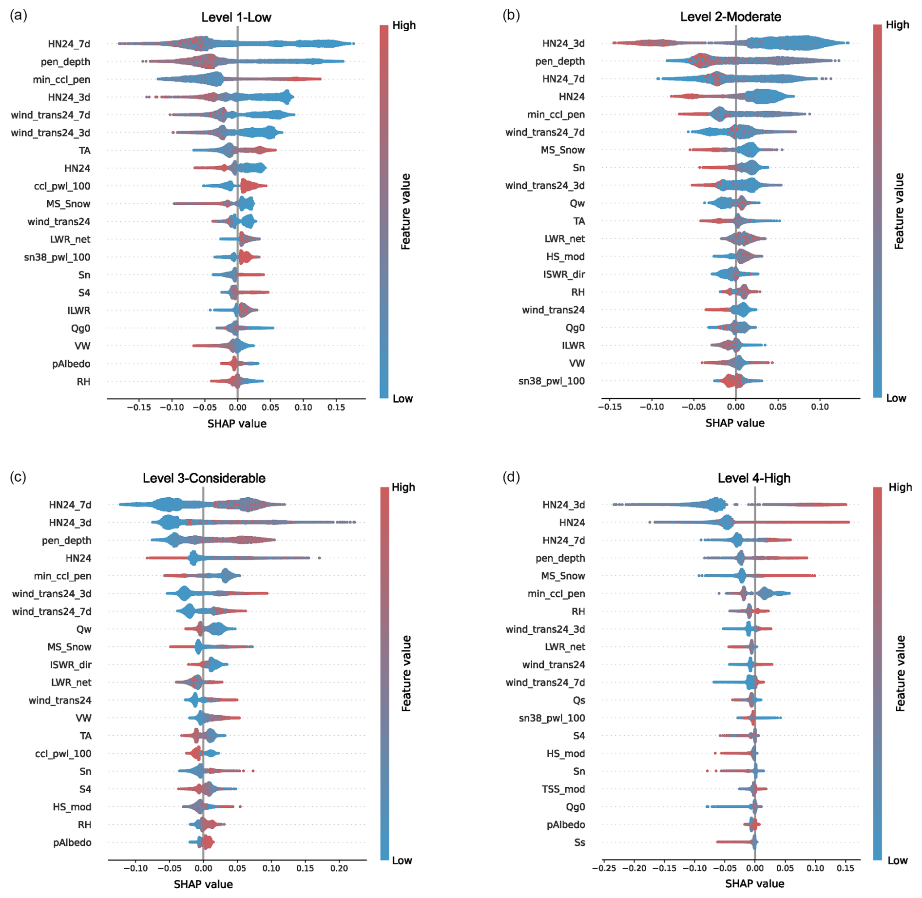
Figure 8 SHAP beeswarm summary of the impact of the 20 most significant features (described in Table A1) on the model output for each danger level: (a) 1-Low, (b) 2-Moderate, (c) 3-Considerable, and (d) 4-High. These features are sorted by importance for each danger level, showing the most significant variables at the top of each plot. The width of the individual charts indicates the density and frequency of SHAP values, thus providing insights into the relative importance of each feature in relation to the model's output. The colour coding (red for high, blue for low) allows us to understand how changes in a feature's value impact each danger level. While positive SHAP values indicate a change in the expected model prediction towards each model's class, negative values denote the opposite.

6.1 Overall explainability

In general, the 3 and 7 d sums of new snow (HN24_7d and HN24_3d in Fig. 8) and the skier penetration depth (pen_depth in Fig. 8) rank among the five most important features, regardless of danger level. Nevertheless, the feature importance order and distributions of SHAP values differ for each danger level.

For danger levels 1 and 2, the SHAP beeswarm charts show that high values of variables related to precipitation (e.g. HN24_3d, HN24, and MS_Snow in Fig. 8 and Table A1) and wind or wind drift (e.g. VW, wind_trans24, and wind_trans24_3d in Fig. 8 and Table A1), as well as the skier penetration depth, negatively impact the model's predictions for these classes. The SHAP distributions of these features are fairly symmetric, especially for danger level 1, indicating that low values of these variables favourably impact predicting these danger levels. Comparing these danger levels, danger level 1 has distinct SHAP distributions for 7 d accumulation of new snow and wind drift (HN24_7d and wind_trans24_7d in Fig. 8), with high SHAP values for low amounts of them. Although these features are also important for danger level 2, the distributions show a wider range of SHAP values with different impacts on the model output. Overall, the model tends to predict low danger levels when the input features related to the amount of new snow accumulated due to precipitation and wind are low. In contrast, for danger level 3 and particularly for level 4, high values of these features have a positive impact (Fig. 8). Precipitation days are also characterized by high relative humidity, which positively drives predictions towards danger levels 3 and 4. The snow precipitation rate, MS_Snow (Fig. 8), is also an important feature for danger levels higher than 1 (Fig. 8). High rates significantly impact predictions towards danger level 4 and help to discriminate between the lower danger levels of 1 and 2 (Fig. 8), which show an inverse distribution of SHAP values. All these are expected results, as high-avalanche-hazard situations for dry-snow conditions are mainly characterized by new-snow accumulation during snowstorms and the formation of wind slabs due to strong winds. In addition, low values of input features such as critical cut length and stability indices represent an unstable snowpack, which may also lead to a high avalanche danger. This is also reflected in the SHAP distributions, where low values of these features (e.g. min_ccl_pen, ccl_pwl_100, sn38_pwl_100, and S4 in Fig. 8 and Table A1) positively impact probabilities for the higher danger levels of 3 and 4, and have a negative impact for the lower danger levels of 1 and 2.

Low danger levels are usually forecast during stable weather conditions, i.e. extended periods with no precipitation and calm and sunny weather (large incoming radiation and high fluxes). The SHAP distributions of low danger levels show that low values of net long- and shortwave radiation and direct incoming shortwave radiation (LWR_net, Qw, and ISWR_dir in Fig. 8 and Table A1) have negative values. Additionally, higher air temperature (TA in Fig. 8) positively influenced predictions towards danger level 1, while lower temperatures drove model predictions towards danger levels 2 and 3. High values of the variables related to the heat fluxes within the snowpack (Qg0 and Qs in Fig. 8 and Table A1) impacted predictions towards lower danger levels, whereas high values of the reflectivity of the snow surface (pAlbedo in Table A1), characteristic of new snow, impacted them towards high danger levels. Therefore, the model tended to predict lower danger levels on days with warmer temperatures and during stable weather conditions.

6.2 Prediction drivers in detail

To gain more insights into the individual impact of the features in the model predictions, we selected an avalanche-forecasting period of interest: March 2021 at Weissfluhjoch (WFJ). During this period, D_bu increased from level 1 at the beginning of the month to level 4 on 16 March, followed by a gradual decrease until the end of the month, when it reached level 2 (Figs. 7a and 9).

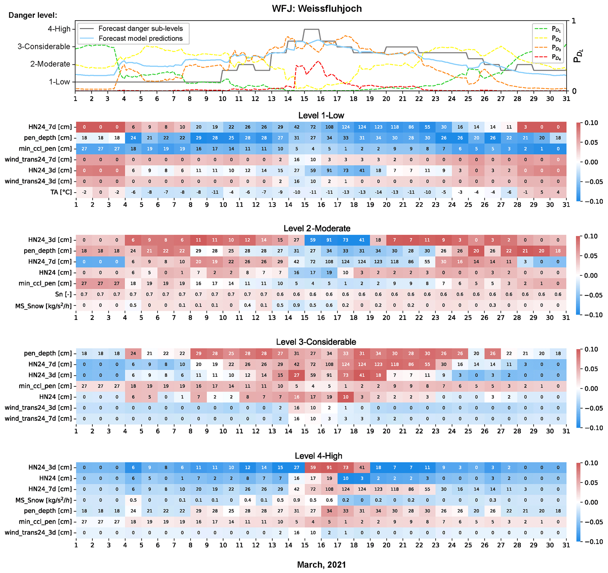
Figure 9 Time series of the sub-levels forecast in the bulletin and the expected danger values, computed with the forecast predictions from the AWS situated in Weissfluhjoch during March 2021 (top; the starting time for each date was set to 18:00 LT). The probability outputs for each danger level during this period are also displayed. Below, the heatmaps show the overall seven most important features for this forecasting period for each danger level (y axis) and the time series of the values for each input feature (x axis). We selected the predictions and input feature values of the time window close to the forecast in the bulletin (starting from 18:00 LT on a given day and valid for the next 24 h). The colour represents the SHAP values computed for each feature in this time window.

The time series of SHAP values during this period shows that the accumulation of new snow was the most important factor across all danger levels (Fig. 9). Approximate thresholds for a given danger level can be estimated by identifying feature values when the SHAP values transition from negative to positive. For instance, at the beginning and end of the month, low snow accumulations during the last 7 and last 3 d (HN24_7d < 14 cm, HN24_3d < 10 cm) resulted in high positive SHAP values for level 1, indicating the highest probability for this level ($P_{D_{\mathrm{1}}}$ in Fig. 9). New-snow accumulations of approximately 10 cm (HN24) and 40 cm (HN24_3d and HN24_7d) had a negative impact (e.g. SHAP values < 0; Fig. 9) on predicting danger level 2. Model predictions increased from level 2 to level 3 when new-snow accumulations exceeded thresholds of 12 cm (HN24_3d) and 20 cm (HN24_7d), approximately. The probability for level 4 was close to zero during the entire month (Fig. 9), except for the period between 15 and 17 March, when $P_{D_{\mathrm{4}}}$ increased. This increase was in line with the bulletin. New-snow accumulations of approximately over 17 cm (HN24), 30 cm (HN24_3d), and 40 cm (HN24_7d) had a positive impact towards predicting danger level 4.

The amount of snow transported by wind (wind_trans24_7d and wind_trans24_3d in Fig. 9) had a similar effect to new snow but with less impact. Wind-drift accumulations over 10 cm in the previous days showed positive SHAP values for high danger levels and negative values for low danger levels. In addition, high rates of precipitation, MS_Snow > 0.4 (Fig. 9), had a negative impact for level 2, while the opposite was the case for level 4.

The month was characterized by large skier penetration depths (pen_depth ≥ 18 cm in Fig. 9), showing increasingly higher negative SHAP values for larger depths at danger level 1. When penetration depths exceeded approximately 24 and 34 cm, the SHAP values were high for danger levels 3 and 4, respectively. The interpretation of the minimum critical cut length (min_ccl_pen in Fig. 9) is more complex since SHAP values show a variety of ranges for the same feature value, exhibiting both positive and negative effects for level 2. For higher danger levels, particularly level 4, critical cut lengths below 20 cm showed positive SHAP values, increasing the probability for this level. However, even though the min_ccl_pen values were low (< 6 cm in Fig. 8) during the period of high avalanche danger forecast from 15 to 17 March in the region of Davos, the impact was lower than that of precipitation variables for danger levels 3 and 4. The values of min_ccl_pen remained low until the end of March, while the forecast danger level remained high with a danger level 3⁻ from 23 to 26 March due to the PWL problem (Fig. 7), and the expected danger value predicted by the model decreased from 2.3 to 2.0 (Fig. 9).

The natural stability index was among the seven most important features for level 2 but with less influence (Sn in Fig. 8). In March, the variation in Sn was minor, showing a low value of Sn ≤ 0.6 (Fig. 9), indicative of an unstable snowpack. Nevertheless, the overall explainability of the impact of this variable for all danger levels is unclear since low Sn values favour levels 2 and 4, while high Sn values favour levels 1 and 3 (Fig. 8).

A remarkable observation regarding the input values of the meteorological features related to the new-snow accumulation is the bias observed between HN24, derived from the COSMO weather model for the next 24 h, and HN24_3d and HN24_7d (Fig. 9). For instance, Fig. 9 (Level 4-High) shows that the HN24_3d value for 16 March is 59 cm, which does not match the sum of HN24 from 14 to 16 March, resulting in 40 cm. These features are computed as a combination of extracted values from the snow-cover simulations driven by COSMO and measured values by the AWS (Sect. 3.1). This explains the differences in the sum of values in Fig. 9 due to an underestimation of precipitation by the COSMO model from 15 to 17 March, which consequently negatively impacted the forecast predictions of the model towards danger level 4. During this period, the expected danger values computed from nowcast predictions were more accurate, approaching danger level 4 (Fig. 7).

7 Discussion

7.1 Model performance during operational testing

We assessed model predictions using the operational test set during the winter season 2020–2021. This was the first winter where the model provided predictions in real time without yet influencing the avalanche forecasters. Although the model was originally trained using data from flat-field snow-cover simulations in nowcast mode, we tested the performance for four virtual slope aspects and in forecast mode. Results show that the agreement rates between the nowcast and forecast danger-level predictions of the model are high, ranging from 84 % to 86 % (Fig. 3), and that the expected danger values are also highly correlated.

Comparing predictions with the danger-level forecasts within the core zone of the bulletin, the overall agreement rate varied from 66 % (flat) to 74 % (south) for forecast predictions (Table 1). While the overall agreement rate for flat-field predictions was lower than previously reported (72 % in  Pérez-Guillén et al., 2022a), the agreement rate for flat predictions per danger level was still similar to that of Pérez-Guillén et al. (2022a). The overall decrease is due to the lower support in the current study for predictions of danger level 1, which typically achieves a high agreement rate, improving overall model accuracy. Predictions outside the core zone showed the expected tendency towards predicting a lower danger level, which is consistent with findings in previous studies (Pérez-Guillén et al., 2022a; Techel et al., 2022) (Tables 1 and B1). This tendency was more pronounced when both the station elevation and the aspect were outside the core zone.

Comparing the expected danger values of the model with the sub-levels as used in the Swiss avalanche forecast, deviations in model performance were mainly concentrated within one sub-level (Fig. C1) and mean absolute errors (MAEs) were below 0.4 (see MAE values for within predictions in Tables 1 and B1). Results are consistent for flat-field predictions and for aspects as well as for nowcast and forecast predictions, supporting the operational use of expected danger values using a rounding strategy as a simple proxy for predicting sub-levels (Techel et al., 2022). Nonetheless, our analysis also showed that model predictions rarely agreed in absolute terms with the sub-levels in the bulletin when avalanche danger was high (i.e. sub-level ≥ 4⁻).

7.2 Interpretation of model predictions

The time series of the model predictions reflected the dynamic nature of avalanche conditions, with a higher temporal resolution than human forecasts, showing rapid increases in avalanche danger (levels) during or shortly after snowfall and more gradual decreases during periods of no precipitation (Fig. 7). However, the model predictions generally decreased faster than the bulletin when a persistent-weak-layer problem was forecast (Fig. 7). Overall, the model performed better during snowstorms, when the new-snow problem was the driving force of instability, and less well in regions characterized by a snowpack with a persistent weak layer (Figs. 6 and 7). This is mirrored in the list of the most important features, which are often related to precipitation rather than to the stability of the snowpack.

7.2.1 Impact of the meteorological features in the model predictions

Among the main meteorological drivers of dry-snow avalanches is the load from snowfall accumulations during or immediately after storms (Schweizer et al., 2003; Birkeland et al., 2019). Consequently, the amount of new snow is ranked as the most important explanatory meteorological variable linked to avalanche activity in previous studies (Ancey et al., 2004; Hendrikx et al., 2014; Schweizer et al., 2009; Dkengne Sielenou et al., 2021; Mayer et al., 2023). The explainability of the model predictions also showed that the meteorological variables related to accumulated sums of precipitation (HN24, HN24_3d, and HN24_7d in Fig. 8) and the skier penetration depth (pen_depth), which is directly linked to new-snow parameters, were the most relevant input features of the model for all danger levels, despite variations in the individual rankings (Fig. 8). These features also ranked highest in the internal feature importance scoring by the random-forest algorithm when developing the model (Pérez-Guillén et al., 2022a). Nevertheless, SHAP values provide a quantitative measure of each feature's impact on the individual model predictions, indicating, as expected, that high accumulations of new snow drive model predictions towards high danger levels, whereas periods of no precipitation or low snow accumulation drive predictions towards low danger levels (Fig. 8). Recent threshold-based binary classification models developed by Mayer et al. (2023) using a subset of avalanche observations in Switzerland predicted days with dry-snow natural avalanches occurring when new-snow accumulations reached thresholds of 22 cm for HN24 and 53 cm for HN24_3d. The detailed explanation of the model predictions at WFJ station (Davos) showed that more than 3 and 17 cm of new snow (HN24) had positive SHAP values, increasing the probabilities for predicting danger levels 3 and 4, respectively. Furthermore, a 3 d sum of new snow of 59 cm on 15 March (HN24_3d in Fig. 9) produced a sudden high increase in the probability of danger level 4. Previously developed statistical approaches to predict natural avalanche activity did not include variables for new-snow accumulations of more than 3 d (Dkengne Sielenou et al., 2021; Viallon-Galinier et al., 2023; Mayer et al., 2023). This study shows that HN24_7d ranked among the most important variables impacting all danger levels, especially danger level 1, when there was no precipitation in the previous week at the beginning and end of the month (Fig. 9). Hence, meteorological variables accounting for precipitation over periods longer than 3 d can also be discriminant features for statistical avalanche forecast models.

Wind is another meteorological factor contributing to dry-snow avalanche formation by transporting snow and producing additional loading in specific areas (Schweizer et al., 2003). In general, the 3 and 7 d wind-drift accumulations ranked between the 10 most important features for all danger levels, while wind velocity and 1 d wind-drift accumulation were less important (Fig. 8). Particularly, the absence of wind-drift accumulations at the beginning and end of March contributed to model predictions trending towards danger level 1 (Fig. 9). The other main meteorological factors that can promote instability in the snowpack are rapid increases in air temperature and solar radiation due to changes in slab properties (Reuter and Schweizer, 2012). In this regard, the input features used by the model are averaged 24 h means of temperature and solar radiation (Pérez-Guillén et al., 2022a) and therefore do not capture rapid changes, resulting in a secondary impact on model predictions (Fig. 8). Over the long term, warming and melting processes favour snow metamorphism and settlement, decreasing the probability of dry-snow avalanche formation (Schweizer et al., 2003). The interpretation of SHAP values is coherent with this, showing positive SHAP values for air temperatures above 0 °C (TA in Fig. 9) and, generally, high values of the radiation parameters for danger level 1 (Fig. 8).

7.2.2 Impact of snow-cover features on model predictions

Besides meteorological drivers, snow stratigraphy plays a crucial role in avalanche formation. A prerequisite for dry-snow slab-avalanche release is the existence of a weak layer within the snowpack (Schweizer et al., 2003). The model was developed with input features extracted from the simulated profiles that contain information on the stability of the snow cover (Pérez-Guillén et al., 2022a). These features include the critical cut length computed at two weak layers (min_ccl_pen and ccl_pwl_100 in Table A1) and several stability indices (Table A1): the natural stability index of two layers (Sn and sn38_pwl_100), the skier stability index (Ss), and the structural stability index (S4). SHAP feature attribution showed that while min_ccl_pen had the highest impact on model predictions, showing that low values positively impacted predictions towards danger levels higher than 1 (Fig. 8), its impact was insufficient to keep high-danger-level predictions at the end of March in the exemplary case due to the PWL problem (Fig. 7). Additionally, the stability indices did not contribute significantly to high danger levels in this avalanche situation. Their impact was not particularly high for any danger level (Fig. 8). Mayer et al. (2023) also tested the development of a classification model using the natural stability index extracted from SNOWPACK simulations to predict natural dry-snow avalanche activity in Switzerland, resulting in low predictive performance. This was mainly attributed to the limited discriminatory power of the natural stability index, which aligned with results from previous studies (Jamieson et al., 2007; Reuter et al., 2022).

In summary, model predictions decreased more rapidly than the bulletin when a PWL was the primary factor contributing to avalanche hazard, suggesting poorer performance due to the low impact of snow-cover stability-related input features. These results are consistent with previous studies linking avalanche problems to modelled weather and snowpack variables in Canada (Towell, 2019; Horton et al., 2020; Hordowick, 2022). However, comparing model predictions to human judgements does not clarify whether the model was inaccurate or whether forecasters were simply too cautious in their forecasts (e.g. Herla et al., 2024). In such cases, using data related to avalanche occurrence or snowpack stability may provide a more objective basis for evaluating predictive performance (Techel et al., 2024).

7.2.3 Model explainability and further implementations

SHAP explanations are a powerful approach for quantifying the overall and individual influence of the input features on model predictions (Lundberg et al., 2018). Compared with other feature-scoring methods, such as variable importance based on Gini importance (Breiman, 2001), SHAP offers a more interpretable analysis of feature contributions. For operational avalanche forecasting, a representation combining the values of the most important input variables with the SHAP values on a daily basis, as shown in Fig. 9, can potentially be very valuable for making a complex machine-learning model understandable for forecasters. This can also be used as a training tool for new forecasters by highlighting relevant parameters and thresholds. Additionally, this approach could be used to detect outliers in the input features, which may lead to incorrect forecasts.

From the perspective of developing new forecasting models based on machine learning, SHAP has confirmed what Pérez-Guillén et al. (2022a) qualitatively showed during the model development: the model's observed performance decreases when the PWL problem is the main avalanche problem forecast. This encourages the implementation of new danger-level models using better discriminant input variables related to snowpack stability, such as the output of the recently developed classifier estimating the probability of potential instability of simulated snowpack layers (Mayer et al., 2022) or the likelihood of natural avalanches occurring (Mayer et al., 2023). As shown in Mayer et al. (2023), using the depth of the decisive weak layer and the probability of instability of this layer extracted from snowpack simulations can help distinguish between danger levels. An alternative could be to develop a model to assess danger levels for each avalanche problem. Nevertheless, this approach could be challenging since several avalanche problems were usually simultaneously forecast on the same day and in the same region (Fig. 7).

7.3 Model integration for operational avalanche forecasting

Since the winter season 2021–2022, the danger-level model has been providing real-time predictions every 3 h. The output includes a danger level (Eq. 2) as well as an expected danger value (Eq. 3) for each weather station, slope aspect, and prediction type (nowcast and forecast). These predictions were accessible to forecasters, who consulted them and compared them with their danger-level assessments to issue the daily avalanche bulletin. In general, model predictions were judged as useful and plausible by avalanche forecasters, providing a valuable “second opinion” in the decision-making process (van Herwijnen et al., 2023). Model predictions were generally considered comparable to the danger-level assessments made by forecasters. One of the model's main strengths is its ability to help identify spatial patterns that are usually challenging to assess. This is especially useful when conditions are rapidly changing and evolving, as shown in Fig. 7. A further recent development is the prediction of a danger level for the predefined warning regions (white-contoured polygons shown in Fig. 1). This approach, described in detail in Maissen et al. (2024) and further adapted and live-tested in 2023–2024 (Winkler et al., 2024), generates forecast predictions including the danger level, sub-level, and the corresponding critical aspect and elevation information in a format equivalent to human-made forecasts, allowing the largely automatized integration of a “virtual forecaster” in the forecast production process (Winkler et al., 2024).

8 Conclusions

In this study, we evaluated the performance of the random-forest classifier predicting the danger level for dry-snow avalanche conditions developed by Pérez-Guillén et al. (2022a) during the initial live-testing season in Switzerland. Although the model was trained with a data set consisting of meteorological measurements providing nowcast snow-cover simulations for flat terrain, its performance was equally good, or sometimes even better, in forecast mode and when making predictions for four virtual slope aspects. Overall, the mean agreement rate between model-predicted danger levels and the danger levels as published in the Swiss avalanche forecast was 70 %. Moreover, the continuous expected danger value, derived using the model-predicted probabilities, showed high correlations (r_p≥ 0.86) with the sub-levels as used by the Swiss avalanche warning service. In general, the model reproduced the temporal evolution of avalanche conditions and captured variations in avalanche danger between different slope aspects and elevations, at higher temporal resolution than that of human-made forecasts. However, the observed performance was lower during periods characterized by persistent weak layers within the snowpack compared to other situations.

Using the SHAP approach, we showed that model explainability can be greatly increased to obtain a detailed understanding of feature importance not only overall, but also for individual predictions. We conclude that SHAP could potentially become a powerful tool permitting the interpretation of the predictions of complex black-box machine-learning models, not just in a research context as shown here, but also when using model predictions operationally. Besides increasing the interpretability of complex models such as the danger-level model, rigorous validation and implementation of these models remain crucial to ascertain that predictions are reliable, which we consider a prerequisite for operational use. Integrating machine-learning models into avalanche forecasting can complement the forecaster's expertise by providing a second opinion. Moreover, model predictions may open up possibilities of increasing the spatiotemporal resolution of avalanche forecasts (Maissen et al., 2024).

Future developments should include incorporating additional discriminant input features (e.g. indices developed by Mayer et al., 2022, 2023), for instance to increase prediction performance for situations with persistent weak layers, or testing the applicability of these models in regions with different snowpack characteristics.

Appendix A: Features of the model

Table A1 Meteorological variables used for training the random-forest algorithm. The three types of features are the measured meteorological variable, modelled meteorological variable by SNOWPACK, or extracted variable. Features can be discarded by recursive feature elimination (RFE), manually, or because they are highly correlated with another feature.

Appendix B: Nowcast performance

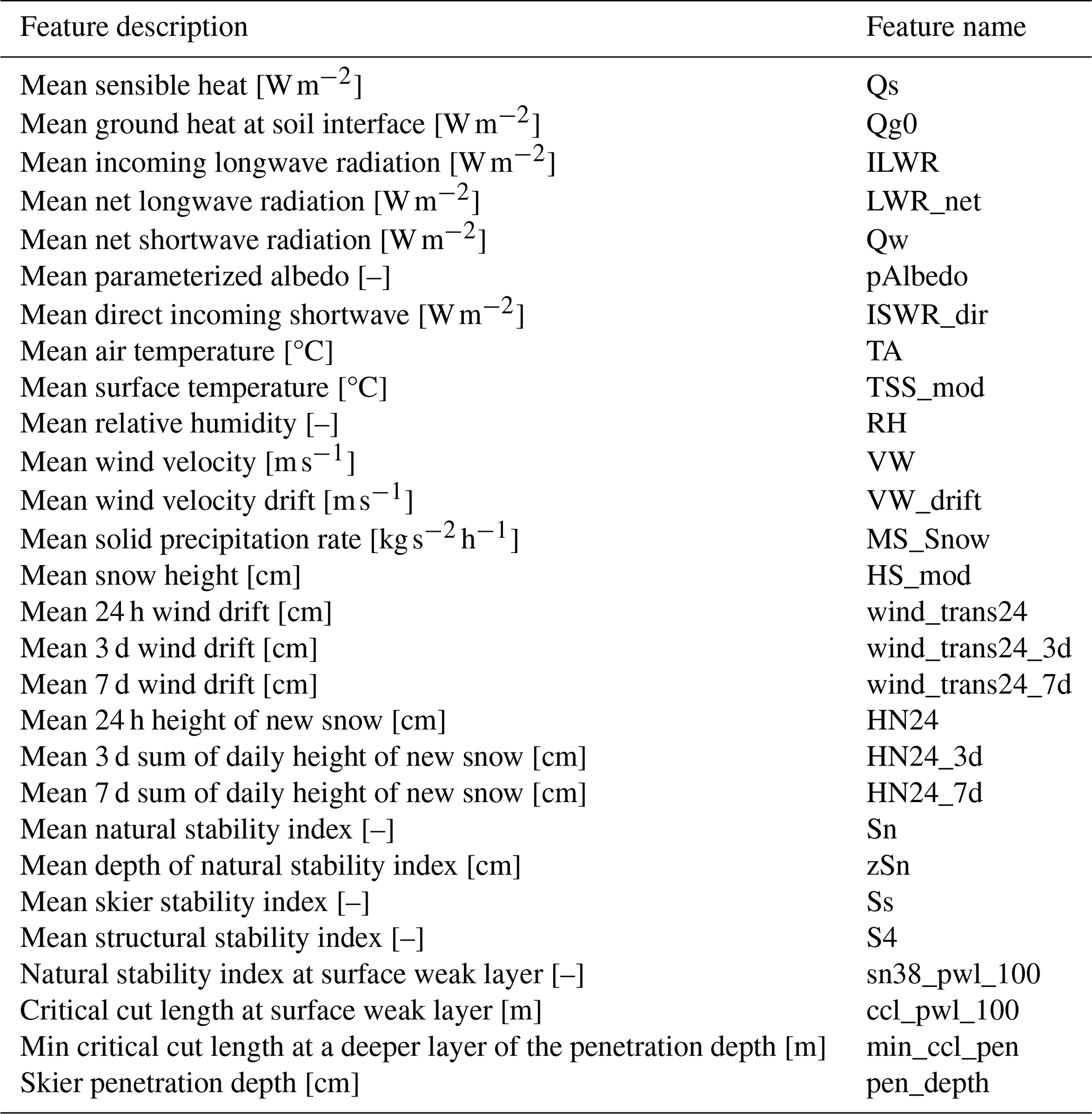
Table B1 Summary of the model's performance during the winter season 2020–2021 based on the nowcast predictions: within (elevation: above; aspects ($\text{F: flat};\text{N: north};\text{E: east};\text{S: south};\text{W: west}$): active +), partly outside (elevation: below; aspects: active +), or outside the core zone (elevation: below; aspects: non-active −); support of the predictions; percentage of samples for each forecast model–bulletin bias (ΔD_bu,a, as defined by Eq. C2), which represents the difference between the danger level predicted by the model and the bulletin. Mean absolute errors (MAEs) and the Pearson correlation coefficient are computed using the expected danger values and the sub-level assessments.

Appendix C: Evaluation metrics

The forecast-nowcast model bias, ΔD_m,a, is defined as

$$\begin{array}{}\text{(C1)}& \mathrm{\Delta }{D}_{m,a}=D_{\text{fx},a}-D_{\text{nx},a},\end{array}$$

where D_fx,a is the forecast and D_nx,a is the nowcast danger level predicted by the model for each mountain slope aspect ($a\in \mathit{\{}\text{F},\text{N},\text{E},\text{S},\text{W}\mathit{\}}$). ΔD_m,a can range from ±3 for a difference of three danger levels in the scale, ±2 for two levels, or ±1 for one level to 0 when the predictions agree. The agreement between predictions is the percentage of the total number of cases where $\mathrm{\Delta }{D}_{m,a}=\mathrm{0}$.

The forecast model–bulletin bias, ΔD_bu,a, is defined as

$$\begin{array}{}\text{(C2)}& \mathrm{\Delta }{D}_{\text{bu},a}=D_{\text{fx},a}-D_{\text{bu},a},\end{array}$$

where D_fx,a is the forecast danger level predicted by the model for each mountain slope aspect ($a\in \mathit{\{}\text{F},\text{N},\text{E},\text{S},\text{W}\mathit{\}}$) and D_bu,a is the danger-level forecast in the public bulletin for each aspect. ΔD_bu,a can range from ±3 for a difference of three danger levels in the scale, ±2 for two levels, or ±1 for one level to 0 when the predictions agree. The agreement between bulletin forecasts and predictions is the percentage of total number of cases where $\mathrm{\Delta }{D}_{\text{bu},a}=\mathrm{0}$.

The mean absolute error (MAE) is the average of the absolute differences between the forecasts and the predicted values:

$$\begin{array}{}\text{(C3)}& \text{MAE}={\displaystyle \frac{\mathrm{1}}{n}}\sum _{i=\mathrm{1}}^n\left|D_{\text{bu},a}^{(-=+)}-{\text{E}}_{D,a}\right|,\end{array}$$

where n is the number of predictions (support in Tables 1 and B1), $D_{\text{bu},a}^{(-=+)}$ represents the sub-levels forecast in the bulletin, and E_D,a is the expected danger values (Eq. 3) predicted for each mountain slope aspect ($a\in \mathit{\{}\text{F},\text{N},\text{E},\text{S},\text{W}\mathit{\}}$).

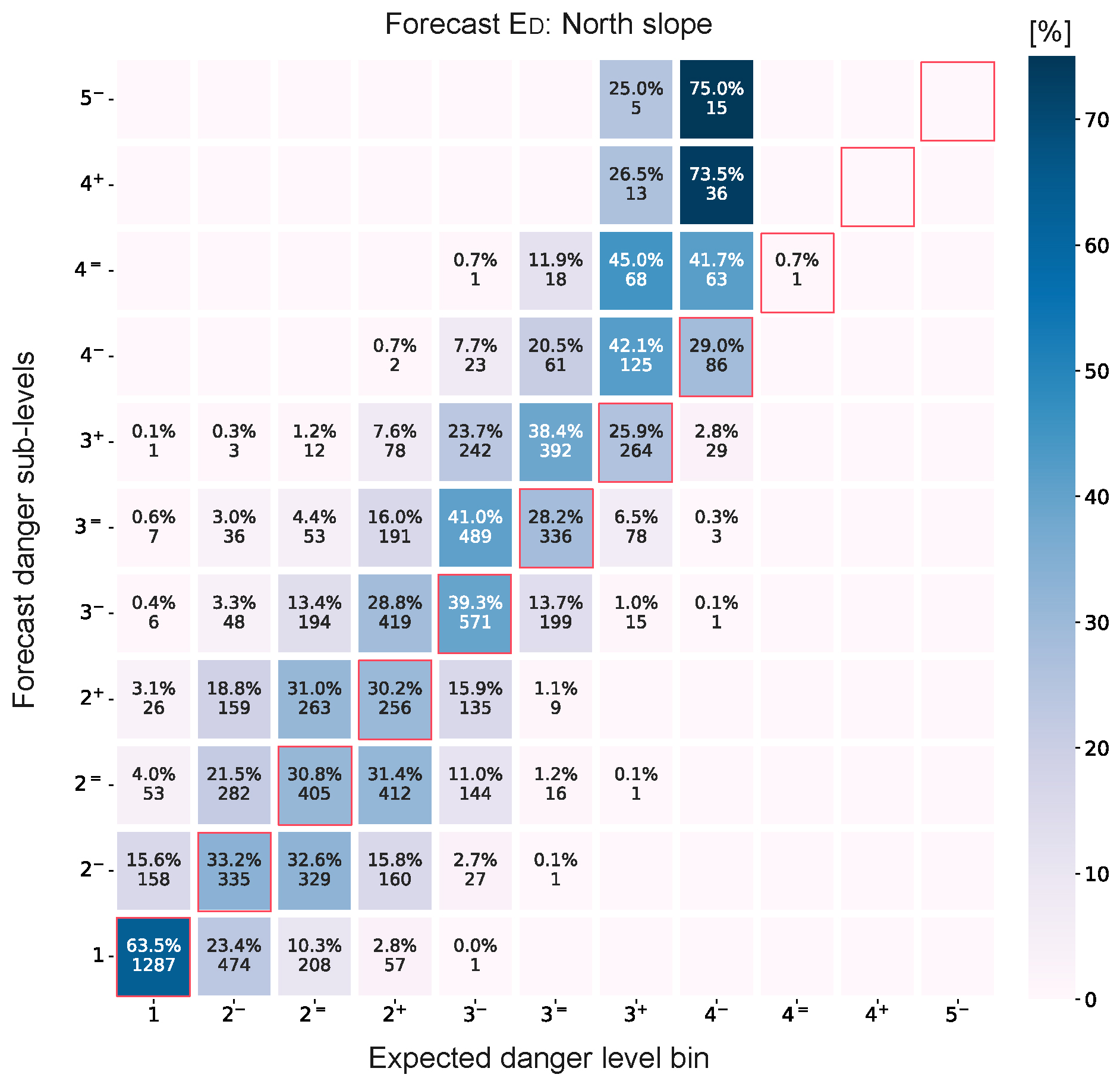
Figure C1 Confusion matrix comparing the sub-levels forecast in the bulletin and the expected danger values (proportion of samples: row-wise sum), which are discretized into refined danger-level scale bins for the forecast predictions.