the Creative Commons Attribution 4.0 License.
the Creative Commons Attribution 4.0 License.
 | 17 Mar 2025
Using random forests to forecast daily extreme sea level occurrences at the Baltic Coast
Kai Bellinghausen
Birgit Hünicke
Eduardo Zorita
We have designed a machine learning method to predict the occurrence of daily extreme sea level at the Baltic Sea coast with lead times of a few days. The method is based on a random forest classifier. It uses spatially resolved fields of daily sea level pressure, surface wind, precipitation, and the pre-filling state of the Baltic Sea as predictors for daily sea level above the 95 % quantile at each of seven tide gauge stations representative of the Baltic coast.
The method is purely data-driven and is trained with sea level data from the Global Extreme Sea Level Analysis (GESLA) dataset and from the meteorological reanalysis ERA5 of the European Centre for Medium-Range Weather Forecasts (ECMWF).
Sea level extremes at lead times of up to 3 d are satisfactorily predicted by the method, and the relevant predictor and predictor regions are identified. The sensitivity, measured as the proportion of correctly predicted extremes, is, depending on the stations, on the order of 70 %. The precision of the model is typically around 25 % and, for some instances, higher. For lead times longer than 3 d, the predictive skill degrades; for 7 d, it is comparable to a random skill. The sensitivity of our model is higher than the one derived from a storm surge reanalysis with dynamical models that use available information of the predictors without any time lag, as done by Muis et al. (2016), but its precision is considerably lower.
The importance of each predictor depends on the location of the tide gauge. Usually, the most relevant predictors are sea level pressure, surface wind, and pre-filling. Extreme sea levels at the meridionally oriented coastlines of the Baltic Sea are better predicted by meridional winds and surface pressure. In contrast, for stations located at zonally oriented coastlines, the most relevant predictors are surface pressure and the zonal wind component. Precipitation did not display consistent patterns or a high relevance predictor for most of the stations analysed.
The random forest classifier is not required to have considerable complexity, and the computing time to issue predictions is typically a few minutes on a personal laptop. The method can, therefore, be used as a pre-warning system to trigger the application of more sophisticated algorithms that estimate the height of the ensuing extreme sea level or as a warning to run larger ensembles with physically based numerical models.
- Article
(5182 KB) - Full-text XML
- BibTeX
- EndNote


Storm surges are extreme and short-lived increases in sea level, mainly induced by extreme atmospheric conditions of wind (e.g. storms) and low-pressure systems (Wolski and Wiśniewski, 2021; Field et al., 2012; WMO, 2011; Weisse and von Storch, 2010; Harris, 1963). They are a major natural hazard for coastal societies, as they can cause not only severe damage to infrastructure on the coast but also the loss of human lives. Hence, monitoring and forecasting systems for storm surges are important to prevent societal damage and to inform decision makers. This study explores the possibility of short-term predictions (a lead time of a few days) of storm surges in the Baltic Sea using a purely data-driven machine learning approach. Technically, the storm surge problem is an air–sea interaction problem, where the atmosphere forces the water body, not necessarily directly at the coast, which in turn responds with oscillations of the water level at various frequencies and amplitudes. While the atmosphere and its wind field influence the currents and wave dynamics of the sea, the currents in turn influence the wave dynamics, which in turn may alter the wind field (Gönnert et al., 2001). Hence, the underlying processes of storm surges are highly nonlinear and often nonlocal, which makes predicting them a complex problem.
Operational forecasting systems of storm surges rely on numerical dynamical ocean–atmosphere models (WMO, 2011; Gönnert et al., 2001). In the Baltic Sea, a few regional models are in operation, such as the BSHcmod from the Bundesamt für Schifffahrt und Hydrographie (BSH), which is a hydrostatic ocean circulation model. While those dynamical models generate reasonable estimations for general water level elevations, they often underestimate extreme (storm surge) events (Muis et al., 2016; Vousdoukas et al., 2016). This is explained by an insufficient grid resolution (Muis et al., 2016), which leads to a misrepresentation of small-scale processes of, e.g. wind fields (WMO, 2011), as well as the underlying ocean bathymetry. Furthermore, the effect of mesoscale weather systems is not well represented in current storm surge models, as no meteorological networks provide data at these spatial scales (WMO, 2011). Usually the data of meteorological fields are interpolated in time and fed into the ocean model (von Storch, 2014), which may lead to too-smooth short-term variability in the atmospheric forcing, which in turn may result in extreme events being underrepresented in the simulations. According to Muis et al. (2016), the underestimation of extreme events can also be explained by the insufficient or missing nonlinear coupling between storm-surge-relevant processes in dynamical models.
Alternatively to dynamical models, forecasting methods can be based on data-driven algorithms. These algorithms are not based on equations representing the physical dynamics but instead try to identify the relevant predictor patterns in a dataset that appear to be associated with a specific predictand. This is achieved by analysing observational datasets of the forcing (atmospheric and/or oceanic) and of the response (storm surge). This makes them more computationally efficient than dynamical models (Harris, 1962) at the expense of being a method that is oblivious to the underlying physical mechanisms and is often more difficult to interpret. Besides the classical statistical methods based on simplified statistical models of the underlying processes, machine learning (ML) is one example of a data-driven algorithm that is becoming more popular in climate sciences. ML algorithms are usually more complicated than classical statistical methods and do not attempt to explicitly or even conceptually represent physical processes but rather try to identify recurring patterns in the data that may be used for predictions. Those complex and non-obvious links between predictors and predictands contribute to their growing application. However, this very complexity makes them more difficult to interpret than classical methods. Also, special care is therefore needed to avoid statistical pitfalls such as overfitting.
Several studies have applied ML methods in order to analyse and predict storm surges, with promising results (Tiggeloven et al., 2021; Bruneau et al., 2020; Tadesse et al., 2020; Gönnert and Sossidi, 2011; Sztobryn, 2003). Statistical and machine learning models were compared when simulating daily maximum surges on a quasi-global scale based on either remotely sensed predictors or predictors obtained from reanalysis products such as ERA-Interim data (Tadesse et al., 2020). The storm surge predictand was derived from two datasets, the observed hourly sea level data from the GESLA (Global Extreme Sea Level Analysis) 2 database and other in situ data of daily maximum surges. They compared linear regression models to a machine learning method called random forests (RFs). The authors found that data-driven models work well in extratropical regions, e.g. the Baltic Sea, and that the ML methods generally performed better than linear regression. Storm surge prediction on a global scale has also been the focus of several ML models, e.g. Bruneau et al. (2020). They show that MLs – in this case artificial neural networks (ANNs) – reconstructed storm surges with significant skill but still struggled to represent the strongest extreme events. Bruneau et al. (2020) explained this by unavoidable limitations of the training data, as extreme events are only a small fraction of the available dataset. Because ANNs are trained with a procedure that is ill-designed for outliers and is biased towards the representation of the average dynamics, extreme surges are difficult to reliably reproduce. Tiggeloven et al. (2021) use a variety of deep-learning methods, a subbranch of ML, to investigate storm surges at 736 tide stations globally. The overall result showed that ML approaches capture the temporal evolution of surges and outperform a large-scale hydrodynamic model. However, extreme events were underestimated for similar reasons as those found by Bruneau et al. (2020).
Most approaches using ML methods are global and, hence, lack specificity for the Baltic Sea basin. The only study (to our knowledge) that applied ANNs specifically to the Polish coast of the Baltic Sea was undertaken by Sztobryn (2003), using preceding mean sea level as well as wind speed and wind direction as predictors of high water levels. The author showed that neural networks can be successfully integrated into operational forecast services, possibly reducing their average error. Similar to the global studies, the study by Sztobryn (2003) showed an underestimation of extreme water levels. Altogether, a thorough application of ML to predict extreme storm surges at several tide gauging stations in the Baltic Sea is missing in the current literature. Hence, we will create a relatively simple RF for the specific storm surge drivers of the Baltic Sea in order to predict extreme storm surges, defined as the top 5% of the highest hourly sea level measurements taken from the Global Extreme Sea Level Analysis (GESLA) 3 project (Haigh et al., 2021). The Baltic Sea is known for its broad coverage by atmosphere and ocean measurements (Rutgersson et al., 2022), and thus it is a very good test bed for ML models.
For the reader that is unfamiliar with the Baltic Sea, we will introduce its specific characteristics when looking at storm surge events. In Sect. 2 we will further specify the underlying datasets of this study as well as their preprocessing. In Sect. 3 the model architecture is presented and the basic principles of an RF are discussed. Furthermore, we will specify how the model was tuned and evaluated. In Sect. 4, we describe all experiments conducted and their rationale, while Sect. 5 summarizes their results. We end the study with a discussion and conclusion.
1.1 Specific characteristics of the Baltic Sea
Apart from the atmospheric forcing, the amplitude of storm surges also substantially varies with specific local conditions such as the topography of the ocean basin, the extent of ice cover, the direction of the storm track crossing the basin, and the shape and orientation of the coastline (Muis et al., 2016; WMO, 2011; Weisse and von Storch, 2010; Gönnert et al., 2001).
Hence, understanding the local characteristics of the Baltic Sea is necessary when building and interpreting a storm surge model. In the following paragraphs, we provide a brief background of the main physical processes that lead to storm surges in the Baltic Sea.
The Baltic Sea is a semi-enclosed intracontinental sea of the Atlantic Ocean that ranges from around 54° N–10° E to 65° N–29° E in northern Europe (Weisse and Hünicke, 2019), as depicted in Fig. 1. It is connected to the North Sea and thus the Atlantic via the Danish straits and the Kattegat. This connection plays an important role in the context of storm surges and tides. The Danish straits block tidal waves and allow mainly internal tides of only a few centimetres within the Baltic Sea (Rutgersson et al., 2022; Wolski and Wiśniewski, 2021). Due to the very narrow connection to the Atlantic, storm surges are only internally induced (Weisse and Hünicke, 2019). The risk of storm surges depends considerably on the location due to the large meridional extent of the Baltic Sea and the different orientation of coastlines in combination with trajectories of pressure systems and wind directions (Hünicke et al., 2015; Weisse, 2014; Rutgersson et al., 2022; Wolski and Wiśniewski, 2020; Holfort et al., 2014).
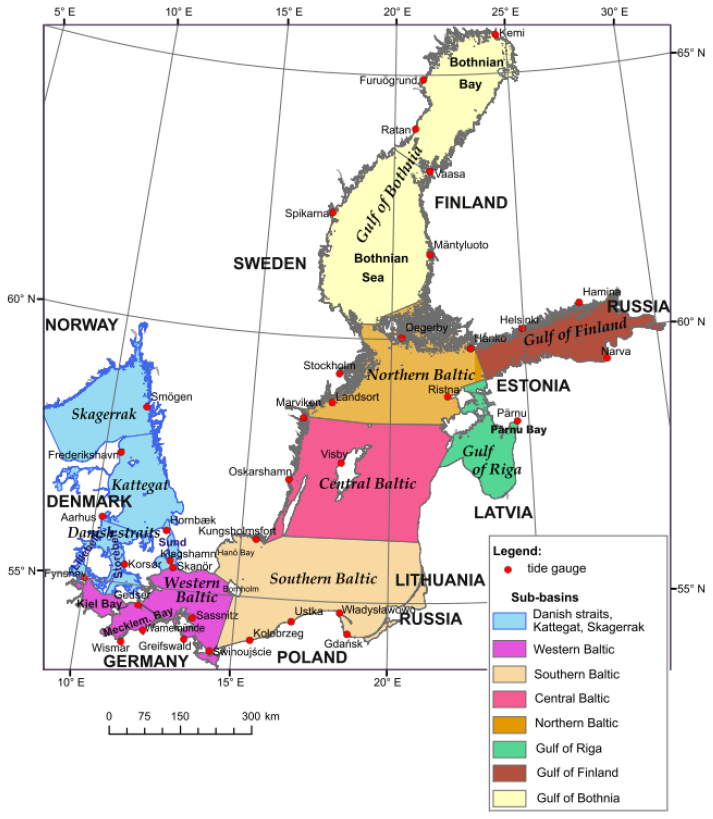
Figure 1Subbasins of the Baltic Sea (coloured) as indicated in Wolski and Wiśniewski (2020). White regions indicate landmasses.
Seasonally, the strongest peaks in water levels are expected from September to February. Those winter half-year surges are mainly driven by processes that alter the volume of the Baltic Sea, e.g. pre-filling (PF) and by the ones that redistribute internal water masses of the basin, e.g. the effects of wind (Weisse and Hünicke, 2019; Weisse, 2014; Hünicke and Zorita, 2006; Chen and Omstedt, 2005).
Due to the Baltic Sea's semi-enclosed basin, specific drivers of storm surges are added to the general drivers such as wind stresses and atmospheric pressure. In the following sections, we provide a brief overview of those drivers.
1.1.1 Wind effect
Storm surges generated by the impact of wind stress are called wind-driven storm surges. If the wind blows consistently over several days, it deforms the sea surface and causes drift currents and wind setup, which eventually lead to a storm surge (Wolski and Wiśniewski, 2021; Harris, 1963). Wind conditions in the Baltic Sea are mainly governed by the westerlies and the cyclonic activity in the northern Europe–Baltic Sea area. This is especially true during the winter months, when the winds are blowing (on average) from south-western directions (Weisse, 2014; Leppäranta and Myrberg, 2009). In periods when the strong westerlies weaken or stop blowing, the elevated sea surface in the north-eastern parts of the Baltic Sea relaxes and water masses rush back towards the southern and south-western coasts. These seiches raise the water levels on the corresponding coasts (Weisse and von Storch, 2010). Furthermore, south-westerly winds, if maintained for several days, can cause a strong inflow of water masses into the Baltic Sea via the Danish straits, leading to a condition of pre-filling (Gönnert et al., 2001). Hence, the wind direction is an important indicator for the onset of storm surges at specific coastlines (Andrée et al., 2022; Wolski and Wiśniewski, 2021).
1.1.2 Atmospheric pressure
In the Baltic region, low-pressure systems are mostly associated with regions of less than 980 hPa (Wolski and Wiśniewski, 2021; Holfort et al., 2014). Those low-pressure systems lift up the sea surface by the inverted barometer effect (Weisse and von Storch, 2010), which eventually induces a baric wave travelling along the trajectory of the system (Wolski and Wiśniewski, 2021). For instance, in hydrostatic equilibrium, a drop in surface air pressure of 1 hPa lifts the sea level by about 1 cm (Wolski and Wiśniewski, 2021; Harris, 1963). As low-pressure systems in the Baltic area usually move from the (south-)west towards the (north-)east during winter, the water surface is more frequently elevated in the north and depressed in the south (Wolski and Wiśniewski, 2021). Wind and pressure combined may amplify the storm surge and increase its intensity, or they may cancel each other out and decrease the severity of the storm surge (Wolski and Wiśniewski, 2021).
1.1.3 Pre-filling of the Baltic Sea
The changing total volume of the Baltic Sea is also important for storm surges. The Baltic Sea contains an averaged volume of 20 900 km3 (Eakins and Sharman, 2010) that is constantly altered due to different in- and outflows (Weisse and Hünicke, 2019). The main inflow is the saltwater exchange of the North Sea and the Baltic Sea via the Danish straits, which is approximately 1180 km3 yr−1 (Leppäranta and Myrberg, 2009). On a daily basis, up to 45 km3 is exchanged between the basins in both directions. Evenly distributing this water mass over the whole Baltic Sea would correspond to a sea level change of 12 cm d−1 (Mohrholz, 2018).
If net water exchange persists over longer periods, the mean Baltic sea level can rise or fall accordingly by larger amounts. If the water level of the Baltic Sea is elevated 15 cm above the mean sea level for more than 20 consecutive days due to increased inflow via the Danish straits, Mudersbach and Jensen (2010) speak of a pre-filling or preconditioning of the Baltic Sea. Usually, water levels at the tide gauging stations in Landsort (Sweden) or Degerby (Finland) are used as proxies to measure pre-filling (Weisse, 2014; Janssen et al., 2001). With a high degree of pre-filling, storm surges can become more likely and more extreme as less wind is needed to induce wind setup (Weisse and Weidemann, 2017; Weisse, 2014). It is mainly the already mentioned south-westerly wind direction that, when blowing over extended periods of time, leads to an increased inflow of water masses to the Baltic Sea through the Kattegat (Wolski and Wiśniewski, 2021; Hünicke et al., 2015; Weisse, 2014). But a sequence of fast-moving low-pressure systems coming from the west and travelling to the north-east of the Baltic Sea can also result in strengthened inflows (Wisniewski and Wolski, 2011). According to Leppäranta and Myrberg (2009), the peak months of inflow are during winter, especially from November to January. Combined with the effects of stronger winds and rainfall in winter, this preconditioning is an important driver of storm surges.
1.1.4 Precipitation
Finally, when low-pressure systems and corresponding cyclones move over the Baltic Sea, they usually bring precipitation along (Leppäranta and Myrberg, 2009; Harris, 1963). Extreme precipitation associated with low-pressure systems is most frequent in winter (Rutgersson et al., 2022). As stated by Weisse and Hünicke (2019), heavy precipitation increases the total volume of the Baltic Sea and changes the density due to a change in salinity profiles, which combined may lead to an increased overall water level. Therefore, the influence of precipitation is not directly related to storm surge magnitudes but rather alters preconditions such as the pre-filling of the Baltic Sea and the filling of rivers and estuaries (Gönnert et al., 2001). Hence, indirect effects of precipitation combined with the onset of a storm surge can lead to severe compound flooding in the Baltic Sea, especially in low-lying coastal areas (Rutgersson et al., 2022; Bevacqua et al., 2019).
The Baltic Sea provides one of the densest tide gauge networks, with records starting in the 19th century (Hünicke et al., 2015), which are a part of the record compilation of the GESLA dataset.
2.1 Area of research
The area investigated ranges between 40–70° N and 5° W–30° E, as depicted in Fig. 2, and includes the Baltic Sea. We intentionally selected a broad region around the Baltic Sea to account for the nonlocal links between the drivers of storm surges and the locality of the event itself. More specifically, seven stations were selected for model analysis. These stations are a part of the GESLA dataset. Station codes are provided in Table A1. This set of stations was chosen to represent all of the coastal orientations and bays of the Baltic Sea.
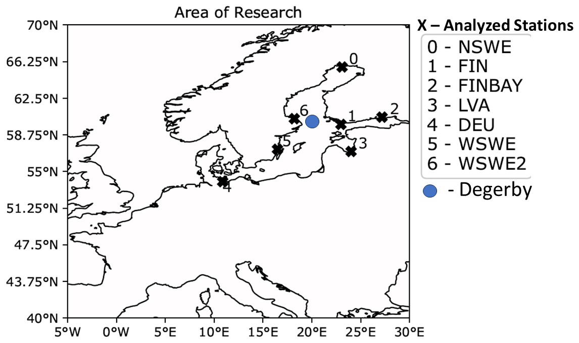
Figure 2Map of the entire research area. Black crosses and numbers identify the stations analysed (predictand) within the Baltic Sea. The closest cities to the stations are Kalix (0, NSWE), Hanko (1, FIN), Hamina (2, FINBAY), Riga (3, LVA), Travemünde (4, DEU), Oskarshamn (5, WSWE), and Forsmark (6, WSWE2). The blue circle indicates the position of Degerby station, which is used as a proxy for the pre-filling predictor.
2.2 Predictand
The GESLA dataset provides a global set of high-frequency (at least hourly) sea level data with integrated quality control flags (Haigh et al., 2021). Height units of all stations were converted to metres, and the time zone was adjusted to Coordinated Universal Time (UTC). A more thorough description of the compilation can also be found in Woodworth et al. (2016) and Haigh et al. (2021). The data are publicly accessible at http://www.gesla.org (last access: 3 November 2024).
All stations that we selected for model analysis contain hourly data covering the period from 2005 to 2018. This sea level data are later used to derive a daily time series of a categorical binary predictand at the respective stations after preprocessing (see Sect. 2.4). The categories of the predictand are either no occurrence of a storm surge (0) or occurrence of a storm surge (1), based on the exceedance of a quantile threshold.
2.3 Predictors
We use spatially resolved fields of daily total precipitation, daily mean wind fields (zonal and meridional), and daily mean sea level pressure from the European Reanalysis 5 (ERA5) data provided by the ECMWF and of daily pre-filling of the Baltic Sea. The ERA5 dataset ranges from 1959 to the present, with daily estimates of atmospheric variables, and is spatially resolved on a 30 km (approximately 0.27°) grid covering the Earth (Guillory, 2017). We select the period from 2005 to 2018 for this study and chose an area that broadly encompasses the Baltic Sea, North Sea, and part of the eastern North Atlantic, which should include the main known drivers of Baltic storm surges. All variables of ERA5 used as predictors are shown and briefly described in Table A2. They are surface pressure (SP), total precipitation (TP), eastward wind at a 10 m height (U10), and northward wind at a 10 m height (V10). Each variable is extracted from the two-dimensional (2D) field depicted in Fig. 2. Additionally, we implemented a predictor of pre-filling using the GESLA time series of sea level data at the station of Degerby. The station is situated at about 60° N and 20.38° E (see blue circle in Fig. 2). The hourly water level at the station of Degerby from the GESLA dataset is used as a proxy for pre-filling and is reduced to a daily time frequency using the maximum recorded water level of a given day as an entry.
2.4 Preprocessing
Initially, we temporally detrend the GESLA time series for each station by subtracting a linear trend in time. We do this for two reasons; one is to obtain a stationary process, which is usually necessary for the application of ML algorithms. Secondly, we subtract the long-term trend from the whole dataset at the beginning in order to cancel out the effects of anthropogenic and vertical land movement on the sea level. The rationale is that the goal of the model is to predict short-term variability in the sea level. We do not expect any issues of data leakage due to this approach, as we also tested the stationarity of each station's time series before subtracting the linear trend using a Dickey–Fuller test. Due to the short time period used here, long multidecadal-scale trends do not impact the analysis.
In a next step we split the GESLA dataset into a calibration set ℳ𝒞, including the time interval from 2005 to 2016, and a validation set ℳ𝒱, including the years 2017 and 2018. The calibration set is later used to fit the ML model, while the validation set is used to evaluate the performance of the model (see Sect. 3). For each of those subsets, we only select months within the autumn and winter season, e.g. months from September through February.
The calibration set is further split into a training set 𝒞train, including the years 2005 to 2013, and a testing set 𝒞test, including the years 2014 to 2016. Hence, we split the calibration set continuously in time, leaving 25 % of the calibration data for the test set.
We then proceed by computing the 95th quantile qtrain of the predictand training set for each station separately. This station-based percentile is used as a threshold to develop the storm surge index for all datasets (e.g. training, testing, and validation sets) and each station. We set every entry containing a sea level strictly below qtrain to 0 (no storm surge) and all remaining entries to 1 (storm surge). This process is visualized in Fig. 3.
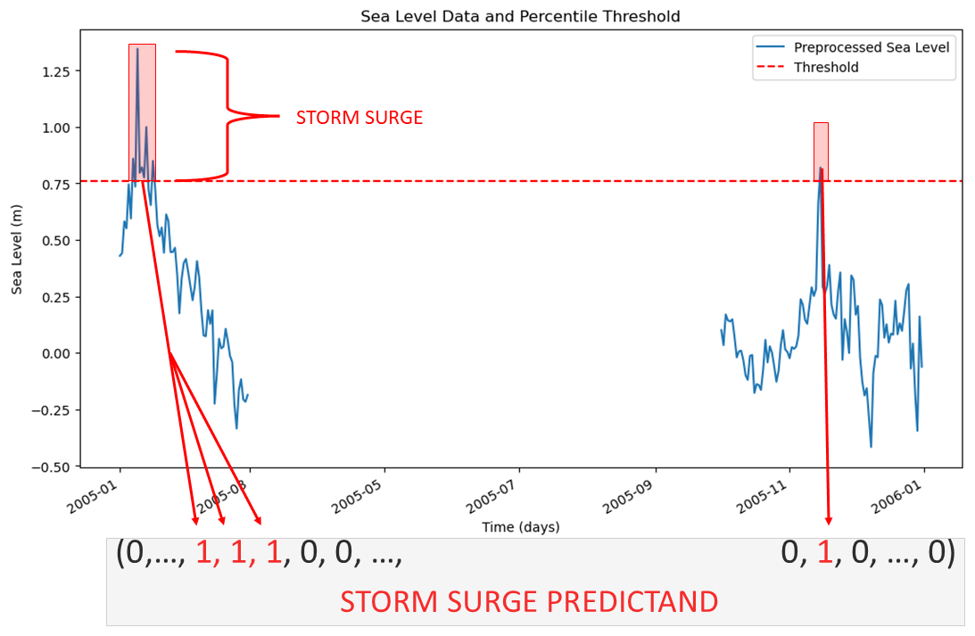
Figure 3Transforming a continuous sea level to a categorical predictand using a percentile-threshold-based definition of extreme storm surges. The predictand is a vector, where 1 indicates a storm surge and 0 its absence.
Doing the steps above, we obtain a time series of hourly temporal resolution for each station, where 5 % of the data is (by definition) classified as an extreme storm surge, and refer to it as the storm surge index. We convert this hourly storm surge index into a daily index by attributing a storm surge to a specific day only if 1 h of that day exceeds the 95th quantile.
Similar to the predictand dataset, we separate the predictor data into a calibration set, which is further split into a training and a test set, as well as a validation set with time intervals identical to the predictand split.
In summary, we obtain the following dimensions for the predictors and predictand after preprocessing.
The ERA5 predictors are two-dimensional spatial maps with a total dimensionality , where npred, n, nlong, and nlat are the number of predictors (drawn from SP, TP, U10, V10), number of samples (days), longitudes, and latitudes, respectively.
The predictand is a categorical binary variable indicating the occurrence of a storm surge with dimensionality n×nstation, where nstation = 1, as we analyse each station separately.
Additionally, the time series of the predictor and predictand are intersected by date to put both on the same time-domain. For some experiments, we introduced a time lag Δt between predictor and predictand by de-aligning the timing of predictors and predictand. In these cases, the number of samples reduces to n−Δt for both the predictor and predictand. Hence for a time lag of Δt any time point, t ≤ n of the predictand is predicted using predictors at prior times t−Δt. To the best of our knowledge, there were no missing values in any of the datasets.
The overall structure of the algorithm is sketched in Fig. 4. Before passing data to the model, we split our predictor and predictand datasets as described in Sect. 2.4. After splitting the data, we feed the model, an RF, identical combinations of predictors for each station. The RF then processes the atmospheric predictors (denoted features in ML parlance) by leveraging the predictions of several decision trees (DTs). Finally, the RF provides a deterministic, binary prediction of extreme storm surges (predictands, also called labels), indicating whether a storm surge occurs (1) or not (0).
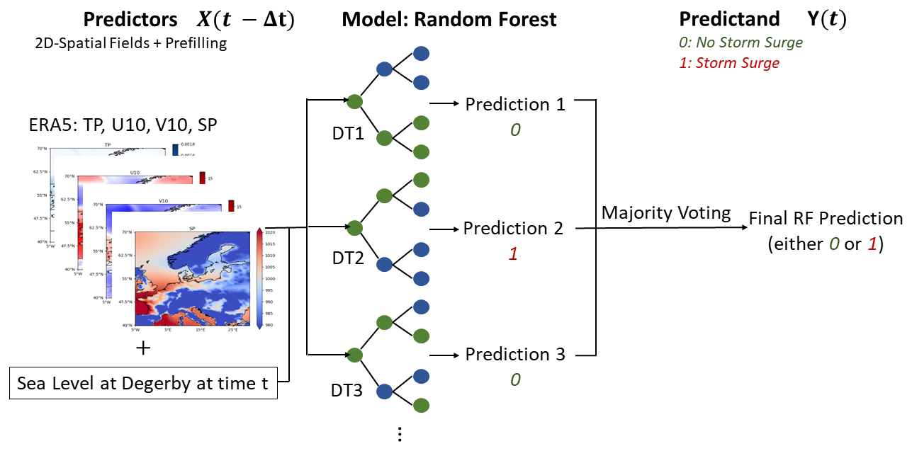
Figure 4Software architecture as a blueprint. A random forest is used to predict storm surges categorically using atmospheric predictors represented as 2D spatial fields.
Commonly, all possible predictors are initially used as inputs for the model. The model can then itself derive the most important features, which comes with additional computational costs. To avoid this circumstance, we only tested combinations of predictors that were in line with the theoretical explanation of storm surges.
Our algorithm is publicly accessible on GitHub (Bellinghausen, 2022) and is based on the scikit-learn library of Python.
In the following sections, we will explain the essential aspects of the RF, its tuning, and its evaluation.
3.1 Random forests
As a classifier, we used the RandomForestClassifier from scikit-learn. A thorough description of RFs can be found in Müller (2017) and Géron (2017), from which we will briefly discuss the most important points.
The model architecture of an RF is based on an ensemble of DTs (see Fig. 4). DTs rely on a hierarchy of if/else questions in order to conclude with a prediction. A simplified example is shown in Fig. 5. In this case, the DT formulates sequential if/else questions about the predictors U10, SP, and PF. The grey nodes indicate a path of input data, where each question is answered positively, thus leading to the prediction of an extreme storm surge. In reality, the questions in each node are more complex, testing for continuous values of the predictor at hand (e.g. U10 > 17 m s−1 as a test for strong west winds at a specific grid point within the research area). When fitting the structure of a decision tree to a training dataset, the algorithm uses a concept called gini-impurity to find the best sequence of if/else questions for a prediction. A prediction based on new predictor data is then made by sifting through the optimized DT, answering all if/else questions.
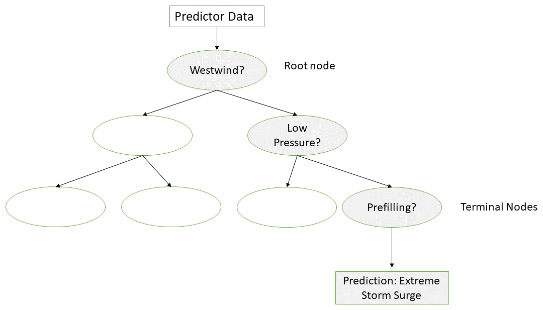
Figure 5Simplified model architecture of a DT. Grey nodes indicate the path of test data while sifting through the DT. Right-pointing arrows refer to positive answers.
In an RF (Fig. 4) as an ensemble of DTs, each of those DTs processes a random sample of the given data in order to reach a prediction. In general, those predictions are then aggregated in order to get the overall prediction of the RF. For a binary classification problem, as in our case, this aggregation is done via majority voting.
Because DTs are based on an if/else hierarchy, RFs belong to the realm of interpretable models, as they provide a parameter f named feature importance (FI). The FI assigns a value between 0 and 1 to each feature (predictor), with higher numbers indicating greater importance. The importance of one predictor is estimated by computing the predictive loss of the algorithm when that predictor is omitted. The value of the importance is normalized by requiring that the sum of all feature importance values within a DT be 1.
In this paper, predictors are atmospheric variables on a grid, which leads to a dimensionality of the feature importance of . Hence, each grid cell is associated with a feature importance for each climate predictor (wind, pressure, etc.), and we can utilize it to filter regions on the grid that are important to the prediction of a storm surge. It is important to note that f should not be mistaken for the causality of a predictor and only represents a (possibly nonlinear) correlation detected by the RF. Hence, we analyse whether the feature's importance resolves regions and atmospheric patterns coherent with the theoretical drivers of storm surges described in the previous sections.
3.2 Model tuning
The RandomForestClassifier can be tuned in several ways by altering its hyperparameters (HPs). We will use the training and testing sets 𝒞train and 𝒞test for this (see Sect. 2.4). The model's internal parameters are optimized based on the training set 𝒞train; the models HPs are adjusted based on the accuracy of the model on the test set 𝒞test, while the models ability to generalize to completely unknown data is investigated using the validation set ℳ𝒱 after the model fit is completed. For an RF, the most important HPs control the number of DTs used (n_estimator), the maximum depth of each DT (max_depth), and the number of features used when calculating the best split (max_features). In general, a larger value for n_estimator will lead to a more robust ensemble due to less overfitting, as the results of many DTs are averaged (Müller, 2017). Breiman (2001) show that the generalization error in RFs converges for a growing number of DTs, again indicating less overfitting. With increasing max_depth, the DTs get more complex; hence overfitting is more likely. The max_features control the randomness of each DT, with a smaller value reducing overfitting (Müller, 2017). While we set the max_features HP to its default value of , we varied the other two.
In addition to those HPs, we altered the class_weight and random_state parameters. The class_weight is used to associate weights with classes. This is particularly important in this study, as we deal with extreme storm surges. Hence, the predictand dataset is unbalanced, as there are many more days of class 0, without a storm surge, than of class 1, with an extreme storm surge. Setting the class_weight to balanced adjusts weights inversely proportional to class frequencies in the input data; i.e. the model will penalize wrong predictions about class-1 days more heavily than wrong predictions about normal conditions. We set the random_state to 0, which gives us and the reader the possibility of reproducing results.
The HPs n_estimator and max_depth were automatically depicted by the algorithm as the best combination of HPs using RandomSearchCV, an optimization procedure within scikit-learn. One can input a list of values for each HP, and RandomSearchCV automatically selects the best combination by optimizing the validation score of the training set based on cross-validation. This comes with the advantage that the initial split into training and testing sets is sufficient, and no additional validation set is needed (for more details we recommend consulting the scikit-learn documentation).
Although the number of effective predictors is substantial, we did not reduce the dimensionality of the predictor fields (by principal component analysis or an auto-encoder) to avoid losing any regional details that could be relevant for each station. We preferred in this case to limit the depth of the random forest algorithm to avoid overfitting, drawing only from the list for the max_depth parameter. For the n_estimator we used 333, 666, or 1000.
All settings are summarized in Table A3 for replication purposes.
3.3 Model evaluation
A common tool to evaluate binary classification models is the confusion matrix (CFM) (see Fig. 6). It summarizes the accuracy of a model in terms of success or failure rates. For our study, we aim for a high true-positive rate (TPR) (also called sensitivity), which relates the absolute number of correctly predicted extreme storm surges (TP) to all incidences of storm surges (TP + FN) in the underlying data. In Fig. 6, for example, TP = 29 out of TP + FN = 40 extreme storm surges were correctly predicted, leading to a TPR of = 72.50 %. A high TPR automatically leads to a low false-negative rate (FNR) since their sum equals 1. The FNR indicates how often the model actually fails to predict a storm surge. With a high FNR, the model can not be trusted, as it very likely produces false predictions of security; i.e. it is too insensitive. Especially for extreme events, this can lead to devastating damage to societies when protection measures rely on model predictions with a high FNR, as eventually no measures are taken due to a model prediction of no storm surge, but in reality, an extreme surge appears.
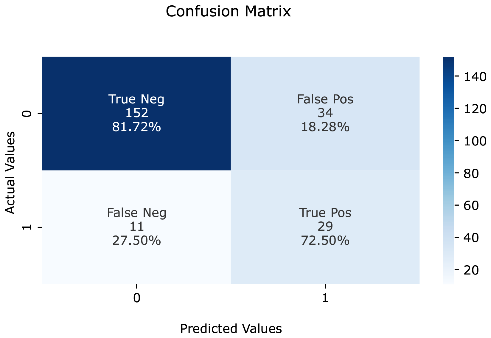
Figure 6Confusion matrix for a binary-classification model with absolute and relative values. The colour bar shows the maximum count of instances for all cases.
The CFM can be evaluated on training and test data as well as on the validation set. If model predictions are almost always correct on training data, i.e. a TPR and true-negative rate of around 100 %, the model tends to overfit. In practice, the CFM of test data and the validation set is more interesting, as it shows the performance of a model when confronted with data that is uninvolved in the training process.
Related to the TPR is the measure of precision. The precision p of a model measures the accuracy of positive (storm surge) predictions and is defined as
where TP and FP count the true-positive and false-positive predictions. It answers the following question: of all instances predicted to be positive, how many are actually positive? For instance, precision of 20 % indicates that, empirically, every fifth prediction of a storm surge is actually a storm surge in the real observations. A perfect model would have p = 1 and hence never predict a storm surge when there was none. This measure is especially important for decision makers if the prediction is used, for instance, to evacuate cities or put protection measurements into place.
Because we are interested in a combination of good precision and good sensitivity (TPR), we will also look at the F1 score. The F1 score combines precision and sensitivity into a single metric using the harmonic mean and is computed by
It penalizes extreme values in either precision or sensitivity, making it a useful metric when there is a need to minimize both types of error equally.
To analyse the relevance of predictors, we will use a combination of feature importance (FI) and a predictor map (PM). For each model, the importance of each feature is displayed by weights between 0 and 1, with all weights summing up to 1. Using FI lets us compare the overall importance amongst predictors when a combination of predictors is input to the model. Furthermore, we can deduce which specific regions within the research area are important for model decisions for each predictor. We only show the top 1 % area of importance (computed by the 99th percentile of FI for each predictor) and depict those regions using grey squares (see Fig. 7).
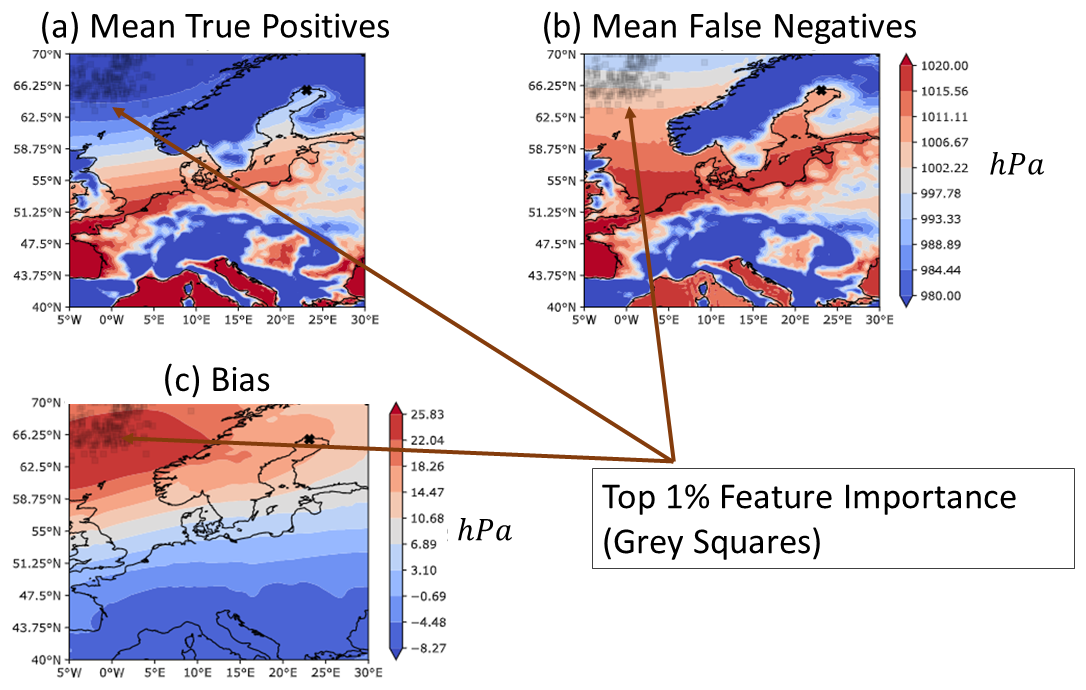
Figure 7Mean predictor maps of SP all with time lag Δt = 1 for NSWE station. (a) Mean true-positive prediction (TPP), (b) mean false-negative prediction (FNP), and (c) the difference in both means, i.e. (b) FNP − (a) TPP. Grey squares indicate the areas of the top 1 % of feature importance. Note the different scaling of the colour bars for the difference maps.
Unlike a correlation coefficient, the FI does not encode the magnitude or sign of the feature that is indicative of the storm surge (Müller, 2017), e.g. whether there is low or high pressure within the area of importance that is related to a storm surge. Hence, in the results we also include an averaged value of the predictor for all cases of a storm surge. This leads to two separate types of PMs: one where the model correctly predicts the storm surge, i.e. true-positive predictions (TPPs), and another where the model predicts no storm surge even though there is one in the observations, i.e. false-negative predictions (FNPs). Those PMs are compared amongst each other in Fig. 7a and b, and their difference (bias) is showcased in panel (c). For instance, when PMs for TPP cases show low-pressure systems in the importance region while the FNP PMs only display high-pressure systems, this suggests that the model heavily relies on low-pressure systems to forecast a storm surge. In contrast, it also suggests that in some cases storm surges are caused even though there are high-pressure systems in the area of high FI.
As it is sufficient to only show maps for TPPs and the difference to FNPs, we will do so in the results section.
We built six overarching model configurations (A–F). For each configuration, we undertake subsets of model runs, which are denoted by run_ids. All model runs are applied to each station; i.e. similar predictors and initial HP lists were used when building the model for each station (note however that the fitted model can be different for each station due to the automatic optimization of hyperparameters). As a starting point, we analysed the predictive skill of each predictor individually with time lags up to 1 week (A). Among those, time lags up to 3 d showed promising results. These time lags are interesting in order to predict storm surges in advance. Hence, we analysed a combination of all predictors (ERA5 and PF) with time lags of 1 and 2 d, eventually getting insight into which predictors are most important (B). In experiment C, we investigate the coupling of strong winds and moving low-pressure systems by combining SP and U10 with various time lags. Because the west wind is an important driver of storm surges in the Baltic Sea due to the connection with the North Sea via the Kattegat and the possible wave build-up in the north-eastern region, we combined multiple time lags of U10 in experiment D. In E we looked into cumulative rain (TP with several time lags and U10), wind-induced waves in combination with pre-filling, and the state of pre-filling induced by wind (both using U10 and PF). Since we use the water level records at the Degerby station as a proxy for pre-filling and not the rolling mean of 20 consecutive days such as was done by Mudersbach and Jensen (2010), we combined several time lags (up to 30 d) of PF in experiment F.
All model runs are summarized in Tables A4 –A9 in the Appendix.
We selected promising results based on the metrics discussed in Sect. 3.3 for the validation dataset ℳ𝒱, where the TPR of this dataset is labelled the validation true-positive rate (VTPR).
The prediction skills described in the following subsections will later be compared in Sect. 5.7 with a storm surge reanalysis obtained from a global comprehensive dynamical model driven by atmospheric forcing from global meteorological reanalysis (Muis et al., 2016). Before that, we can provide a basic benchmark by indicating the prediction skill of a simple uninformed prediction scheme. One such scheme could be to always predict storm surges. This scheme would display a true-positive rate of 100 % but also a false-positive rate of 95 %. Hence, it would be very sensitive but very unspecific. A prediction scheme that always predicts no storm surge would display true-positive and false-positive rates of 0 % each. It would be totally insensitive. Both schemes are obviously not useful. A slightly more sophisticated scheme would issue a storm surge prediction randomly on 5 % of the occasions. The true-positive rate would amount to 5 % and the false-positive rate to 5 %. It would still be rather insensitive. A prediction scheme has to clearly improve on this random sensitivity and specificity.
5.1 A – single predictors and multiple time lags
We aim to find the best predictors for each station and analyse what time lags are most useful. Furthermore, we want to investigate how physical patterns of predictors change depending on the station location by investigating their feature importance.
5.1.1 Surface pressure (SP)
In terms of VTPRs, the SP leads to good results for all stations except DEU. For most stations, it worked best if no time lag was introduced, but for LVA station time lags up to 3 d were applied without reducing the TPR below 70 %. The highest VTPR of 81.48 % amongst all stations were seen for WSWE station and a time lag of 1 d. In general, increasing the lead time substantially decreases VTPRs. Amongst all stations (except DEU), the precision is slightly above 20 %, and F1 scores are slightly above 30 %. For instance for LVA station, using a lead time of 3 d comes with precision of 21.34 % and an F1 score of 32.7 %. The overall highest precision of 34.48 % and an F1 score of 45.9 % were also obtained for LVA station with a lead time of 1 d. Independent of the station, low-pressure systems are important within the area of importance (AoI), but for cases of FNPs, the pressure rises several hPa. At NSWE station, for example, the AoI of SP is within the region of 62.5–70° N and 5° W–5° E (see Fig. 8). Here, mainly low-pressure systems with lower than 990 hPa lead to a correct prediction of a surge. The model tends to produce FNPs once the pressure in the AoI increases by a mean of around 25 hPa. In some cases, high-pressure systems of more than 1020 hPa occurred in the AoI for FNPs. This behaviour repeats at several stations.
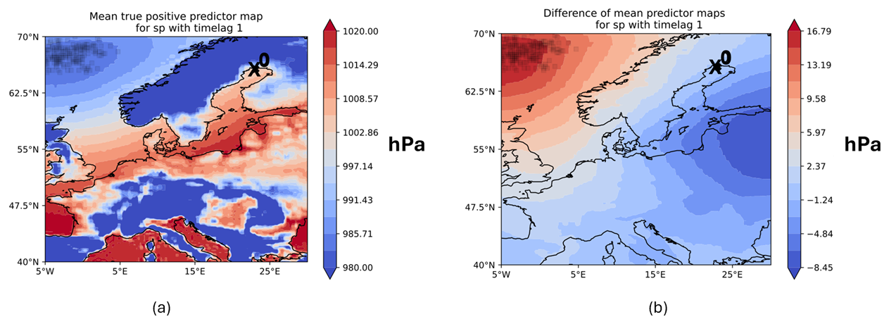
Figure 8Mean predictor maps of SP with Δt = 1 for NSWE station for (a) TPPs and (b) the difference in FNPs and TPPs. Note the different scaling of the colour bar for the difference maps.
5.1.2 Zonal wind (U10)
The zonal wind component was mostly useful for stations at zonal extents of the Baltic Sea coastline. For instance, for FINBAY, a VTPR of 78 % and precision of 24.5 % were achieved when using no time lag. For a lead time of 1 d, a VTPR of 82.76 % with precision of 38.09 % and an F1 score of 52.17 % was computed for LVA station, which were the overall highest scores amongst all stations. Multiple lead times up to 2 d were also useful for WSWE2 station, but the VTPR drops from 82.76 % without a time lag to 67.86 % for a time lag of 2 d.
The AoI depends on the location of the station as well as on the chosen time lag (see Fig. 9). When no time lag is used, the AoI tends to be closer to the station of interest or in a region where it is able to induce wave setup (see the left column of Fig. 9). For instance, for FINBAY station, strong west winds in the AoI will lead to more water masses pushed into the bay, which will eventually lead to a storm surge at the station location.
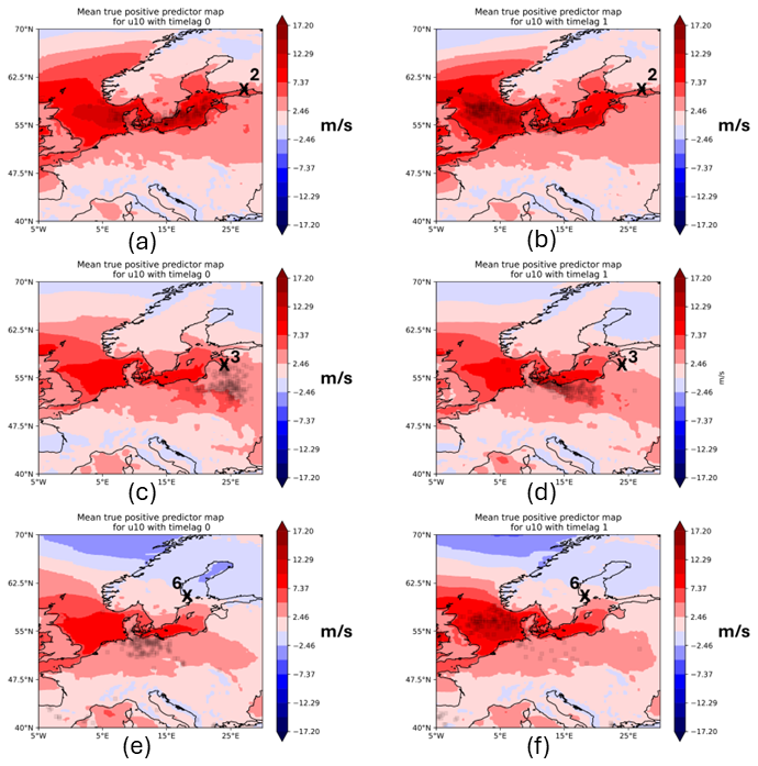
Figure 9Mean predictor maps for TPPs using U10 with lead times of 0 (a, c, e) and 1 d (b, d, f) for stations FINBAY (a, b), LVA (c, d) and WSWE2 (e, f).
Interestingly, the AoI shifts significantly when the lead time is increased to 1 d (see the right column of Fig. 9). West winds become more important in the North Sea close to the entrance of the Kattegat, which could be connected to the condition of pre-filling, as water masses are being pushed into the Baltic Sea by these type of winds.
Regardless of the AoI's location, the main wind direction is eastward. For instance, at FINBAY station, mean west wind speeds of around 12 m s−1 occur in parts of the AoI for TPPs, especially around the Kattegat. When looking at PMs separately, wind speeds of 17 m s−1 and more (i.e. storms) were able to be detected. Comparing the maps of TPPs to the ones of FNPs, one can see that the model generally leads to false predictions when west wind fields become weaker. The difference maps show a mean decrease in west wind speeds of around 7 m s−1 in parts of the AoI (not shown). Hence, the model is not as reliable when west winds are not strong and no winds or even east winds occur. This behaviour repeats for other stations except for DEU station. Here, the east wind is used for model predictions (see Fig. 10), which is an expected result. There are fewer (positive) storm surges on the German coast of the Baltic Sea compared to other bays, as usually south-westerly winds lower the water level in those regions (Weisse and von Storch, 2010). It is interesting to see, however, that important short-term winds are mostly westward in proximity to the station. This is also theoretically explained by the induced pile-up effect of wind at this station. Another previously mentioned driver of storm surges along the German Baltic coast is seiches. These might be induced by the pronounced west wind around the station and over the Baltic Sea for a time lag of 7 d (Fig. 10b). The long time lag could be sufficient for wave growth towards the opposing coast, which in turn leads to seiches once the wind turns westward or stops blowing. Note, however, that these results need to be taken cautiously, as the evaluation metrics are low for DEU station, and the AoI is also widespread.
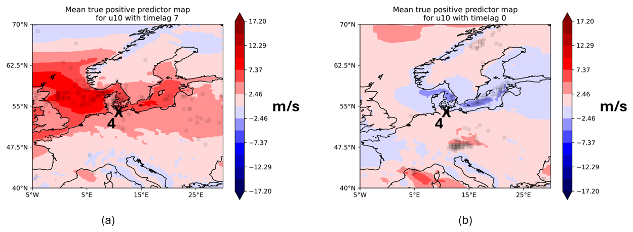
Figure 10Mean predictor maps for TPPs using U10 with lead times of 0 (a) and 7 d (b) for DEU station.
5.1.3 Meridional wind (V10)
While the zonal wind is a good predictor for stations located at the zonal boundaries of the Baltic Sea, the meridional wind component V10 is mostly a good predictor for stations located at the meridional extents of the Baltic Sea. The predictor – with lead times up to 2 d – was useful for all stations except for FIN station. For instance at NSWE station, a VTPR of 69.44 % was achieved with precision of 40.32 % and an F1 score of 51.02 % when using no time lag. For DEU station, a lead time of 1 d results in a VTPR of 68 %, precision of 41 %, and an F1 score of 68 %, which was the highest F1 score amongst all stations. For WSWE station, a lead time of 2 d resulted in a VTPR of 66.67 %, which dropped significantly compared to a VTPR of 74 % when no time lag was used. At this station a lead time of 1 d has a VTPR of 70 %, precision of 21 %, and an F1 score of 32 %. The predictor maps for NSWE, DEU, and WSWE stations are shown in Fig. 11 for time lags of 0 and 1 d. Similar to the zonal wind component, the AoI of the meridional wind component is close to the station when no lead time is used and moves away with increasing lead time. It is also interesting to see that the direction of the meridional wind component switched depending on the location of the station. For instance, for NSWE and FINBAY (Fig. 11a–d), winds blowing towards the station, i.e. northward, are important, while for stations at the southern extents of the Baltic Sea, a southward wind direction is important (Fig. 11e–h). Interestingly, at NSWE, mainly light south winds of around 6 m s−1 are seen within the AoI for TPPs. There is also a notable shift in the patterns of V10 when increasing the lead time. For instance, for DEU station, the AoI is close to the station for no lead time, and the southward wind fields are extended over the whole Baltic Sea. For a lead time of 1 d, this pattern shifts, and the strong wind fields over the Baltic Sea reduce while they are stronger over the North Sea, even north of the UK, eventually pushing water masses into the Kattegat. A similar pattern shift was observed when looking at the predictor maps of FINBAY (see Fig. 11c) and comparing them to NSWE station. The northward wind fields are more localized close to the station instead of reaching the whole Baltic Sea and even into the North Sea. This could be explained by the fact that FINBAY is situated far into the Gulf of Finland, where local winds directed at the station become more important, while NSWE faces more open water masses of the Baltic Sea in a meridional direction. In summary, V10 can be used for all stations except FIN; depending on the station's location, the wind direction used for predictions shifts. The model struggles when no meridional winds blow in the AoI or when their direction is opposite, facing away from the station's location.
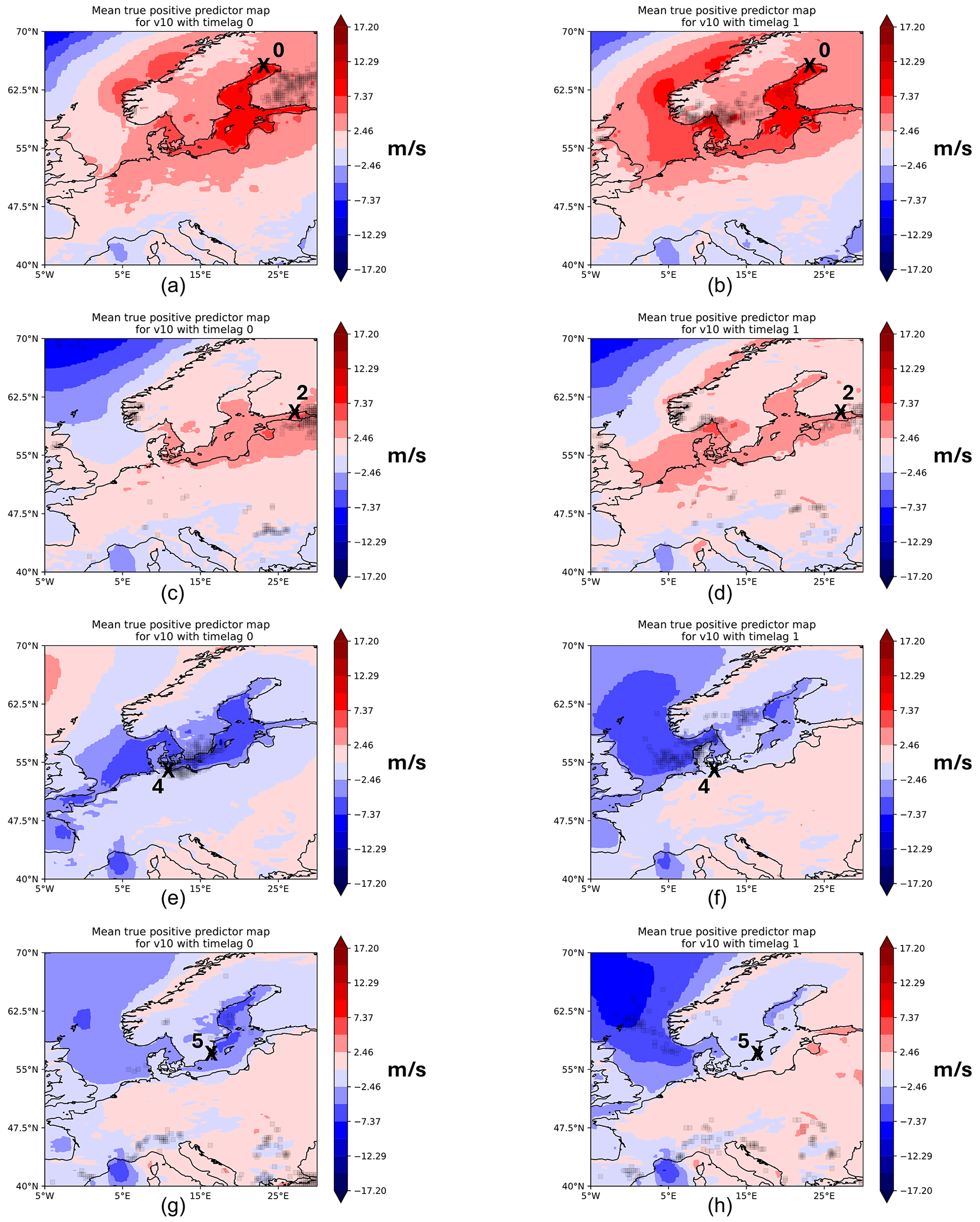
Figure 11Mean predictor maps for TPPs using V10 with lead times of 0 (a, c, e, g) and 1 d (b, d, f, h) for NSWE (a, b), FINBAY (c, d), DEU (e, f), and WSWE (g, h) stations.
5.1.4 Total precipitation (TP)
Total precipitation was overall not a good predictor and only worked for FINBAY, LVA, and WSWE2 stations. For FINBAY station, it was only a relevant predictor with a lead time of 0 d. For WSWE2 station, lead times of 1 and 2 d had a VTPR of 71.43 %, each with precision around 21 % only. Interestingly, for LVA station, even a lead time of 6 d resulted in a VTPR of 74 %, precision of 22.7 %, and an F1 score of 34.7 %. The overall highest F1 score of 41.6 % was obtained for LVA station and a lead time of 1 d.
There is a recurring pattern for the AoI when using TP without a time lag. Usually, it is close to the station itself, as depicted in Fig. 12. When increasing the time lag by only 1 d, the AoI shifts towards the area around Bergen, sometimes showing connecting patterns of importance across the North Sea towards the United Kingdom. Nevertheless, throughout all experiments, TP did not show any consistent patterns in terms of PMs and hence is not considered a relevant predictor (at least in this model setup).
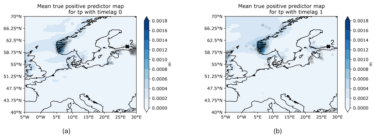
Figure 12Mean predictor maps of TPPs for predictor TP with time lags of 0 and 1 d.
5.1.5 Pre-filling (PF)
Compared to the ERA5 predictors, the pre-filling predictor contains a significantly smaller amount data (one data point per time step compared to a 2D spatial map of around 17 000 entries). Despite this simplicity in data volume, it works reasonably well for all stations except NSWE.
Similar to ERA5 predictors, the model is sensitive but not very specific for some stations when PF is used as a predictor, especially with increasing lead time. Despite this fact, PF is the predictor with the highest precision and F1 score in this experiment. For WSWE2 station, those maximum values in precision and F1 score were 60.52 % and 68.6 %, respectively, when pre-filling was used without a time lag.
Pre-filling is the only predictor that has consistent precision above 20 % for lead times longer than 3 d. The VTPRs are above 70 % even for longer time lags, but increasing the lead time comes at the cost of diminished precision. For instance, for FINBAY station, the precision and F1 score for a lead time of 3 d are 43.8 % and 55.8 %. For LVA station, lead times up to 1 week have precision slightly above 20 %. For instance, for a lead time of 7 d, the VTPR, the precision, and the F1 score are 74.07 %, 20.4 %, and 32 %, respectively.
From experiment A, we can conclude that the choice of predictors depends on the station at hand. Depending on their location, values of predictors in the AoIs vary, especially when considering wind fields. For SP the model always uses low-pressure systems in order to achieve TPPs. For the wind fields U10 and V10, the important wind direction depends on the station location. In general, time lags up to 3 d could be useful, but increasing lead times often leads to worse results. Overall, PF was the most useful predictor for all stations. The results are summarized in Fig. 13.
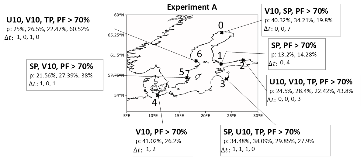
Figure 13Summary of best predictors per station for experiment A. The bold percentage indicates the VTPR. We denoted the best precision and the time lag of the corresponding predictors in order below each set of predictors.
Since the occurrence of storm surges also depends on the interaction between predictors, we will test combinations of predictors in the following experiments.
5.2 B – combination of all predictors
In this experiment, we combined all ERA5 predictors in order to rank them by feature importance and look at the behaviour of their corresponding PMs. In addition, we introduced time lags of either 1 or 2 d to all predictors (see Table A5). Figure 14 shows that for almost all stations, SP and U10 are the most important predictors. They again show pronounced low-pressure fields (below 980 hPa) and strong west winds (greater than 15 m s−1) in their respective AoIs. This behaviour switched only for the stations at the Baltic Sea's meridional extents (DEU and NSWE), where V10 becomes important as well. In terms of PMs, the physical components did not change compared to experiment A.
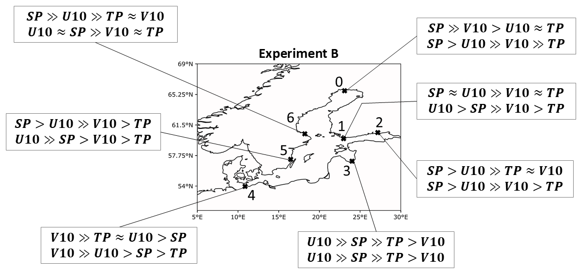
Figure 14The order of predictor importance for experiment B. The first and second rows show time lags of 1 and 2 d, respectively. The >> sign indicates that the feature importance was almost twice as high; the ≈ sign indicates approximate equality.
Nevertheless, using the predictors in combination showed an order of importance, as depicted in Fig. 14. We can see that SP and U10 are mostly used by the models, but it also switches depending on the station and time lags. In terms of the maximum VTPR achieved at each station, using isolated predictors leads to better results.
5.3 C – coupling of U10 and SP
We already noted that SP and U10 are important predictors. In theory, resonance coupling of strong winds and moving weather systems (low-pressure systems) leads to extreme storm surges as well. Hence, we will now investigate two sets of combinations of those predictors, as shown in Table A6. One set uses similar time lags for both predictors and the other uses a shorter time lag for SP compared to U10, as we expect the effects of U10 on storm surge to be slower than the influence of low-pressure systems. This is due to the fact that U10 needs to transfer kinetic energy to the ocean's surface first in order to induce waves.
We summarized the best combinations in terms of VTPR in Fig. 15. For NSWE and FIN, the combination without a time lag worked best. For FINBAY multiple combinations worked. The best combination was a mix of short- and long-term information on both predictors, leading to a VTPR of 80.65 %, precision of 28.4 %, and an F1 score of 42 %. Interestingly, even a lead time of 6 d for both predictors had a VTPR of 71.88 % and precision of 23.9 %, while the importance for SP and U10 were at 68 % and 32 %, respectively (not shown). For LVA station, short-term information on U10 is most important, and VTPRs are generally above 70 % if a lead time of 1 d is used for U10 within the combinations. For the best combination, the VTPR, precision, and F1 score were 85.19 %, 42.59 %, and 56.7 %. As expected for DEU station, no combination worked well. Interestingly, for WSWE station, the long-term info on U10 is most important for the model prediction. The best VTPR, precision, and F1 score are 72 %, 30.5 %, and 42.8 %, which were achieved when combining the short- and long-term information of the predictors.
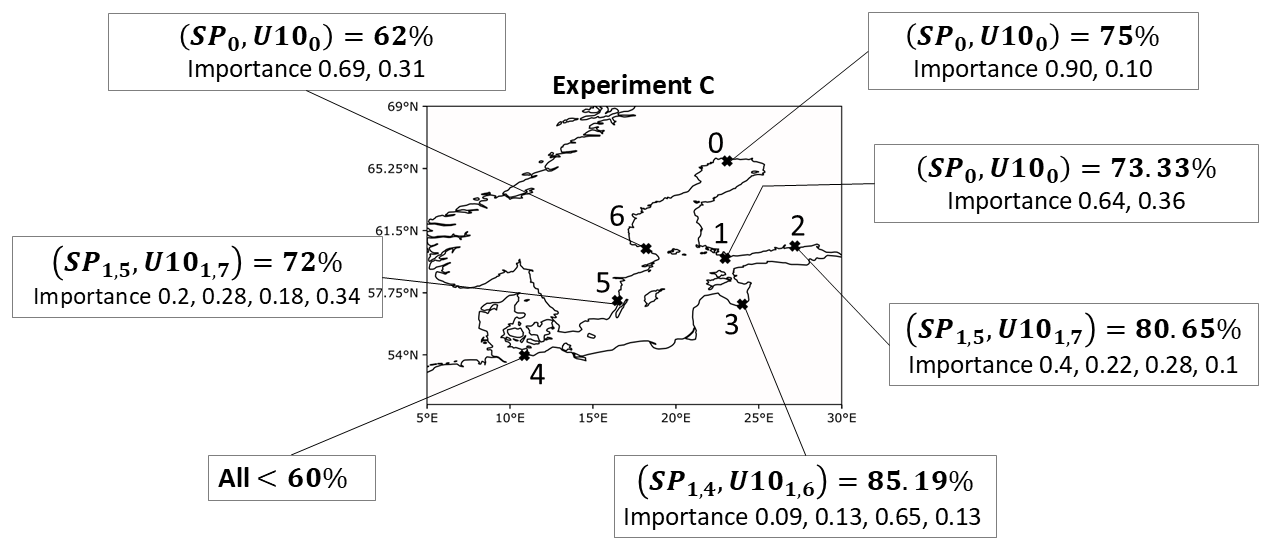
Figure 15The best combinations of predictors in terms of VTPRs for experiment C. Time lags are indicated as subscripts of the predictor. Importance values are given by the order of subscripted time lags.
The PMs mainly showed similar behaviour as when using isolated predictors.
Comparing VTPRs across all stations of both subsets of this experiment, we deduce that similar VTPRs over 70 % and, in the best cases even up to 85 %, were able to be achieved.
In total, this experiment showed that, for most stations, a combination of short- and long-term data, as well as a positive difference in time lags between U10 and SP, leads to good results in terms of VTPRs.
5.4 D – combinations of west wind–time lags
As was already shown, west winds are an important driver of storm surges. If those winds blow consistently over several days, it deforms the sea surface and causes drift currents. Hence, in this experiment, we will investigate U10 with several time lag combinations, as shown in Table A7.
We combine short-term time lags with longer ones in the first subset of this experiment (run IDs 0–3). In a second subset, we investigated time lags up to 1 week, comparing short- and long-term combinations of the time lag (run IDs 4–7). Finally, we spread the time lags over a whole week and even over a whole month for run IDs 8–11.
The results in terms of best VTPRs are shown in Fig. 16. For NSWE, no combination worked well. This is in accordance with results from previous experiments, where the zonal wind is not an important predictor for this station. For FIN station, the best VTPR was 73.33 % but with a low precision of only 13.25 %. Hence, U10 alone is also not a good predictor for this station, at least for the combinations that were used within this experiment. For FINBAY station, multiple combinations of U10 come with VTPRs above 70 %. The best precision was around 33 % with an F1 score of 45 % for a combination of lead times of 1, 7, 14, and 21 d. Interestingly, even for lead times of 5, 6, and 7 d combined, the VTPR was 71 % with precision of 22 %. For LVA station, the combination of short- and long-term U10 works well and leads to increased precision and F1 scores. For instance a VTPR of 81.48 %, precision of 38.5 %, and F1 score of 52.3 % were achieved when lead times of 1, 3, 5, and 7 d were used in combination. As expected, combinations of U10 only are not useful for DEU station. For WSWE and WSWE2 stations, VTPRs were close to 70 % but only for one combination. Nevertheless, it is interesting to see that the longest time lag comes with the highest feature importance for those stations. This could be an indicator that, for those stations, the pre-filling of the Baltic Sea plays a major role, as water masses could be pushed into the Baltic Sea by the zonal winds with longer lead times.
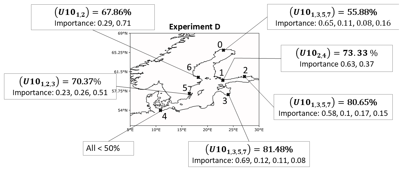
Figure 16The best combinations in terms of VTPRs for experiment D. Importance values are ordered by subscripted time lags.
AoIs and PMs again show similar behaviour to the previous experiments, i.e. mainly strong west winds mostly in regions around the Danish straits or the southern Baltic coastline. AoIs vary depending on the location of the station. They do so even for slight positional changes in stations, for instance, WSWE and WSWE2 stations. Figure 17 depicts this for a time lag of 2 d. While for WSWE2 station, the west winds around the North Sea entrance of the Danish straits are important, this is not the case for WSWE station. The whole AoI shifts more eastwards. One explanation might be that west winds cannot induce a direct wind setup for WSWE2 station, as its coastline is oriented towards the north and hence sheltered from the winds. The opposite is true for WSWE station. The coast here faces southwards and south-westwards. Hence, west winds may induce strong wind buildup for WSWE station, while for WSWE2 station, a state of pre-filling is induced by the wind around the Danish straits, which indirectly leads to a storm surge. In summary, combinations of U10 can be used for most stations as a good predictor when focusing on time lags up to 4 d (see Fig. 16). For some stations, time lags up to 1 week also lead to good predictions. Longer time lags should not be used, as they are mostly disregarded by the model.
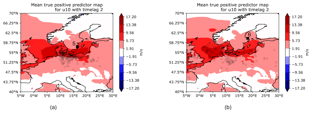
Figure 17Mean predictor maps for TPPs using U10 with a time lag of 2 d at (a) WSWE and (b) WSWE2 stations.
5.5 E – predictor combinations from theory
We tried to emulate the effect of cumulative rain and looked into how information on pre-filling changes the behaviour of the west wind for model predictions. The combinations of predictors can be found in Table A8, and the results of VTPRs are summarized in Fig. 18.
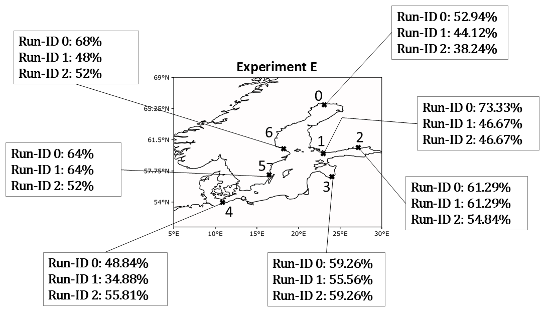
Figure 18VTPR results for all stations and run IDs from experiment E.
The best results for the cumulative rain combination (run ID 0) were observed for FIN and WSWE2 stations with VTPRs of 73.33 % and 68 %, respectively. For FIN, LVA, and WSWE stations as well, good results around 60 % VTPR were calculated. However, when looking at the importance, one can see that U10 is mostly used for model predictions. For all stations except NSWE, the sum of TP feature importance is smaller than the feature importance of U10.
Using combinations of zonal wind U10 and PF were not useful for any of the stations. We expected that the information of the pre-filling would lead to a model that relies on zonal winds that are weaker compared to model runs where U10 was used as a sole predictor, but this was not the case.
5.6 F – combinations of pre-filling–time lags
The pre-filling of the Baltic Sea is strongly influenced by the strong west wind. While Weisse (2014) as well as Mudersbach and Jensen (2010) defines the pre-filling as the rolling mean of the water levels at Degerby over 20 consecutive days, we will use a time lag of the records of the water level at Degerby as the predictor. In this experiment, we investigate PF as an isolated predictor for time lags up to 1 month, as well as combinations of PF that include short-term (up to 1 week) and long-term (up to 1 month) information on the water levels. All combinations can be found in Table A9, and results are summarized in Fig. 19.
For NSWE and FIN stations, pre-filling did not work very well as a predictor. For FINBAY, PF works reasonably well for multiple combinations instead. The best precision of around 30 % was achieved for the combination of time lags of 5 and 10 d, as well as when combining multiple time lags of 3, 14, 21, and 30 d. The VTPRs are 70.97 % and 87.1 % for those combinations, respective to time lags of 5 and 10 d. The importance of a lead time of 3 d is highest (66 %), but additionally, the long-term information accounts for more than 30 % of the total importance. For LVA station, there are high VTPRs of around 81 % for a time lag of 10 d. The precision for this lead time is below 20 %, however. The precision increases when adding short-term information on the pre-filling, for instance, for the combination of time lags of 5, 15, and 25 d, the precision is 26.31 % and the VTPR is 74 %. For DEU station, PF is also a useful predictor. The best combinations are those with lead times of 5, 15, and 25 d, coming with precision of 22.8 % and a VTPR of 70.73 %. When looking solely at VTPRs, a lead time of 10 d works best. For WSWE station, VTPRs are comparably low, only around 70 % for most combinations. The highest precision of 27.86 % was achieved when using lead times of 5, 15, and 25 d combined. Similar to WSWE station, the VTPRs of WSWE2 station are around 70 %. The highest precision of 24.32 % was computed for a combination of lead times of 5 and 10 d.
Pre-filling seems to be a good predictor overall for almost all stations when combining information from the most recent water records with records up to 2 weeks old. Independent of the station, combining several time lags of information works better in terms of precision than using the information in isolation. The fact that the feature importance of short-term lead times was generally higher indicates that the model heavily relies on the most recent water level recordings in order to provide TPPs. Nevertheless, the additional information regarding multiple longer lead times was not neglected by the model.
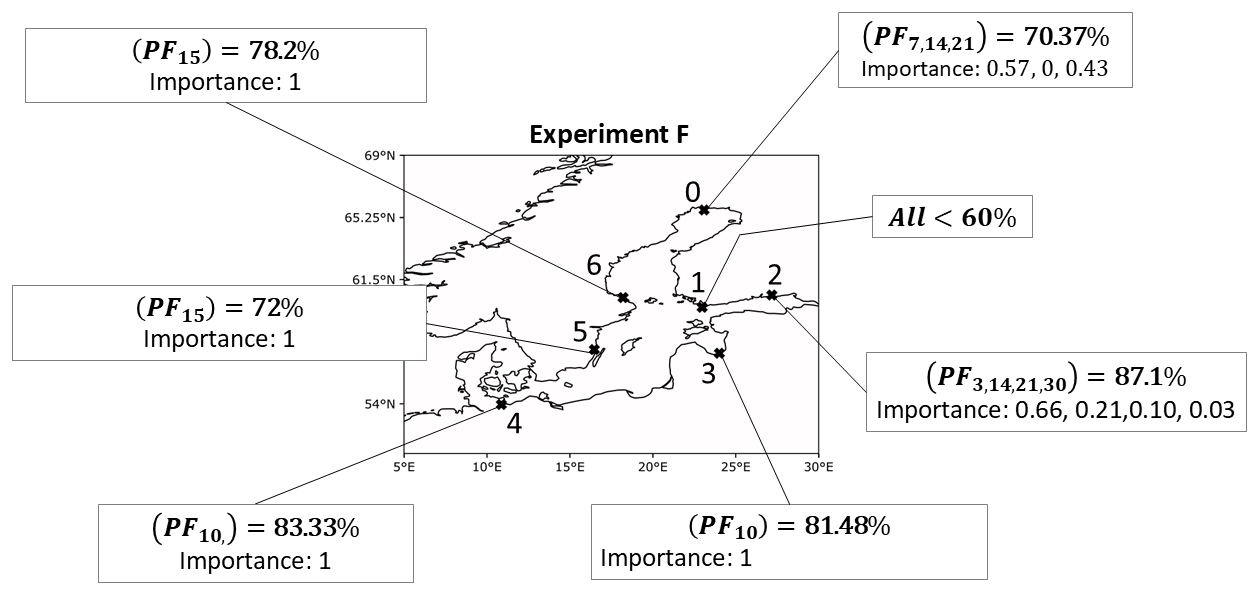
Figure 19The best combinations in terms of VTPRs of PF for experiment F. Importance values are ordered by subscripted time lags.
5.7 Benchmark
Ideally, we should compare the performance of the random forest algorithm with storm surge predictions obtained using hydrodynamical models driven by the atmospheric forcing. There are, however, several obstacles to this comparison. For a fair comparison, the hydrodynamical predictions for day t should be driven only by information available up to day t minus the time lag, with varying time lags or at most including numerical weather predictions up to day t. Those predictions, probably conducted by the respective hydrographic services of the different Baltic countries, are not available to us. Instead, we benchmarked our random forest algorithm against a hydrodynamical modelling storm surge reanalysis that, in principle, should be superior since the predictors used by the storm surge dynamical model include all the information available in the predictors without any time restrictions, even after day t, as the family of ERA atmospheric reanalyses are based on a 4D-Var (4D-variational) data-assimilation scheme (Hersbach et al., 2020).
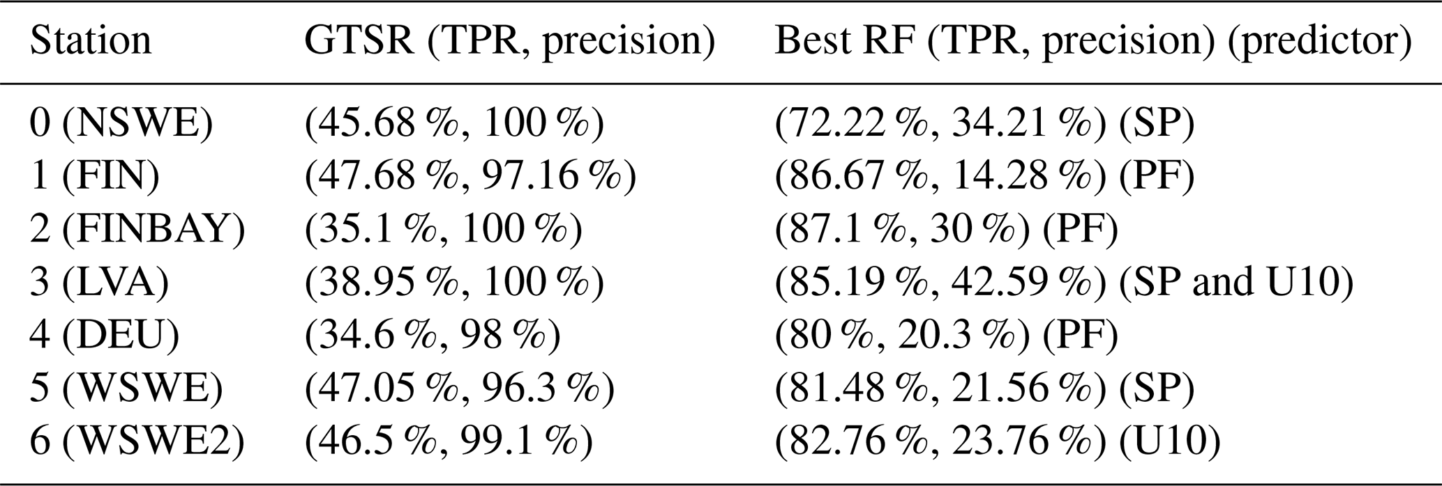
The storm surge reanalysis that we used as a benchmark is the global reanalysis of storm surges done by Muis et al. (2016). Based on hydrodynamic modelling, they presented the first global reanalysis of storm surges and extreme sea levels (the GTSR dataset). Their model is driven by the meteorological reanalysis ERA-Interim. The spatial resolution of ERA-Interim is very close to the resolution of ERA5, from which we extract the atmospheric predictors. We preprocessed the GTSR dataset and consider it to be a prediction of extreme storm surges, comparing it to our preprocessed categorical GESLA dataset as a ground truth by computing corresponding CFMs.
The GTSR dataset consists of several model grid cells along the global coastline with a daily temporal resolution. For each of the stations in our research, we selected the closest model grid cell within the GTSR dataset. The GTSR we were able to download only contained the months of October to March, from which we selected the months of October to February, which overlap with our target months within the GESLA dataset. We use the index that we developed based on the GESLA data as a ground truth; e.g. this index is based on the detrended GESLA data that are further classified by the percentile thresholds given by the training set 𝒞train (see Sect. 3). To ensure that both datasets are in the same time domain, we intersect the GTSR time period with the GESLA index. We then apply the same preprocessing steps to the GTSR data that we also imposed on the GESLA data. Hence, we proceed by linearly detrending the GTSR dataset and finally classify it using its own 95th percentile as a threshold. This ensures that the GTSR storm surge prediction is consistent with its own amplitude of simulated sea levels. This leads to two datasets with a daily temporal resolution that contain categorical entries indicating whether a storm surge occurs at a specific time or not. We consider the preprocessed GTSR dataset to be predictions of extreme storm surges and the GESLA dataset to be the ground truth when computing the CFMs. The resulting TPRs and precision of the GTSR dataset are compared to the best VTPR of our study in Table 1. The results confirm the previous findings by Muis et al. (2016), namely that extreme storm surges are often underestimated by GTSR in terms of TPRs. For all stations analysed in this study, our ML approach performs better than the GTSR in identifying storm surges. In contrast, the GTSR is more precise than our model. Almost every time that it issues a storm surge prediction, there is a storm surge in the observations.
Table 1Comparison of the TPRs for the GTSR prediction and the RF prediction based on the validation set ℳ𝒱. We selected the best RF in terms of the highest VTPR amongst all experiments.
The theory indicates that one predictor alone should not be sufficient to describe storm surges. The main features are the wind stress and the low-pressure systems (below 980 hPa), as well as their speeds. Our models showed good results when using isolated predictors but also worked well when using them in combination. Furthermore, for almost all stations (except NSWE and DEU stations), surface pressure and the west wind were the most important ERA5 predictors. Our model results suggest that mostly low-pressure fields below 980 hPa and strong (mean) west winds of 10 m s−1 around the area of the Danish straits lead to TPPs, especially for stations located in the north-east of the Baltic Sea. For those stations, the AoI of U10 was situated south of the Danish straits, reaching inland towards central Germany. This can actually be explained by predominant south-westerly winds in winter months, which eventually push water masses towards the north-east. Furthermore, PMs showed (when looking beyond the AoI) that those strong west winds often acted over a long horizontal distance, which according to Weisse and von Storch (2010) increases the potential of storm surges. It is this wind direction that leads to the fact that U10 and SP did not lead to any good predictions for DEU station. This is theoretically sound, as for stations in the south-west of the Baltic Sea, water is pushed away towards the north-east due to winds and baric waves. In contrast, those stations should be more subject to low extreme sea levels, which we did not investigate in this study.
For stations at the meridional extents of the Baltic Sea, the meridional wind component should be the most important predictor. We saw that, for instance, for NSWE and DEU stations, where northward and southward winds were a predominant factor for storm surges, respectively.
According to Leppäranta and Myrberg (2009), the largest amount of precipitation is found on the eastern coast of the Baltic Sea due to the winds blowing mostly eastward in wintertime. We were not able to reproduce this in our model. If any structure at all could be obtained from AoIs of TP, it was the importance around the area of Bergen and the UK. Also, the corresponding PMs of TP did not show stronger rain on the eastern coast of the Baltic Sea. In contrast, Gönnert et al. (2001) state that the influence of precipitation is not directly related to storm surge magnitudes but rather alters preconditions such as the pre-filling of the Baltic Sea and the filling of rivers and estuaries. For almost all stations, this was actually true. Compared to other ERA5 predictors, PF generally led to better TPRs on the validation set.
Sometimes our model showed patterns for AoI and PMs that, however, were hard to explain using theory. For instance, for NSWE station, low-pressure fields in the European North Sea were of great importance instead of low-pressure systems close to the station (see Fig. 8). This behaviour showed up mainly when using time-lagged predictors. Theoretically, low-pressure systems in those areas move towards the east, i.e. in the direction of the station, which might be one possible explanation. Additionally, for some cases, storm surges were observed but not predicted (FNPs) – for instance in the presence of high-pressure fields. This behaviour was not due to SP being a sole predictor, as we were able to observe the same behaviour when accounting for a combination of all predictors. The time lag of the predictors might have been too long, such that high-pressure systems were able to move past the station, giving way to a low-pressure system before the actual day of the storm surge. One idea to overcome this problem is to use hourly gradients of atmospheric pressure as predictors, which indicate a rapid (de-)intensification of low-pressure systems (similar to Bruneau et al., 2020).
Nevertheless, we saw that time lagging the predictors improved model results for some stations. This is in alignment with Tyralis et al. (2019), who showed that random forests worked better when time-lagged predictors were used. In general, time lags up to 2 d worked quite reasonably, while longer time lags did not add much value to VTPRs. For instance, a lead time between 1 and 3 d for U10 was often the best choice. This is what we expected, especially for north-eastern stations, as deep-water waves need approximately 2 d to travel across the Baltic Sea. For PF, mostly short-term time lags work best, but still, it was even possible to increase the time lag up to 1 week. This contradicts the actual definition of pre-filling, and one might argue against the usage of the plain time series of water recordings at Degerby as a plausible predictor.
When comparing the relatively high VTPRs obtained from all experiments to their corresponding precision, we can infer a general pattern of our model; it is sensitive but not as precise as the storm surge reanalysis. As mentioned before, this comparison is not fair, as the drivers for the benchmark storm surge model use complete temporal information before and after the storm surge. Nevertheless, this is an important caveat, especially when considering this model for decision making. Models used for decision making should be precise, ideally having precision of 100 %. Hence, at this stage, the model should be improved before it can be used in a decision making process, and we instead advise using it as a surrogate model that can be used as a trigger to run more precise models for operational storm surge predictions. Alternatively, the hydrographic agencies may compare the sensitivity of our model with their operational predictions to evaluate any possible gains of this approach.
Other caveats of our model need to be mentioned as well. First of all, we only use a period of 6 months over 12 years to generate training and testing data. But Bruneau et al. (2020) showed that for machine learning, and specifically artificial neural networks, 6–7 years of daily training data are necessary. In order to overcome this, one could extend the dataset to longer time periods. Using more data increases computing time, which is one reason why we did not implement it. Our main objective was to design a relatively simple prediction scheme that would not need heavy computing resources. However, in view of the results obtained, the algorithm could be trained using more data with more powerful resources.
Furthermore, algorithms trained with predictors based on remotely sensed data outperformed algorithms trained with predictors obtained from the reanalysis data by Tyralis et al. (2019). We used only reanalysis data as predictors. If remotely sensed data are available, testing the algorithm with them could provide better statistics.
For future studies within this context, it would be interesting to alter and specify some of the predictors. For instance, instead of only using U10 and V10, one could actually calculate all of the wind stresses, i.e. the wind direction, wind velocity, and its duration. Our dataset did not involve the duration, which is especially important for the generation of surface waves and swell. Similarly, if low-pressure systems move at relatively high velocities, i.e. greater than 16 m s−1, a sub-pressure-driven storm surge occurs (Wolski and Wiśniewski, 2021) because the effect of the baric wave is stronger than that of the wind. We did not use the speed or the trajectory of a low-pressure system as model input. However, these can be important as they induce resonance coupling and give direction to the induced baric wave. Another physical change that can be made is to look at negative storm surges instead of positive ones and see if the behaviours of U10 and SP change for stations such as DEU. For instance, the bays of Mecklenburg and Kiel experienced strong negative storm surges due to water outflow caused by low-pressure systems moving towards the east (Wolski and Wiśniewski, 2020).
From a technical perspective, one could adjust the definition, i.e. the binary encoding of storm surges, to represent the alarm levels at specific stations instead of using percentiles. To improve the precision of the model, one could also alter the loss function of the RF such that it penalizes false-positive predictions more heavily. Ideally, this would increase the precision and F1 score and make the RF more suitable for direct operational usage. This could, however, worsen the sensitivity.
It would also be interesting to extend the usage of the RF to random regression forests in order to investigate and predict the actual heights of the water level during storm surges. Further, Tiggeloven et al. (2021) showed promising results using deep-learning methods when those models are tailored for specific regions. However, predictions over the whole range of variations are more complex and may require either more data or more computing power. Additionally, a more common approach in the ML literature is to supply all the input predictors considered for the RF model and let the model itself decide which combinations and connections are important. We did not apply this and instead backed the choice of predictors with the underlying theory of storm surge development. Hence, we only tested combinations of predictors that were in line with the theoretical explanation of storm surges. We then wanted to infer the spatial patterns of physical predictors within the research area and their importance compared to each other.
In this study, we designed a prediction scheme for the occurrence of storm surges, i.e. the top daily 5 % of coastal water levels, for seven stations across the Baltic Sea. The prediction horizon is a few days, and the method is based on a random forest used as a binary classifier. The method was tested on records of the water level at stations from GESLA3, and atmospheric predictors were taken from the ERA5 dataset, from which we choose variables of surface pressure (SP), zonal (U10) and meridional (V10) wind speeds at 10 m above the Earth's surface, and total precipitation (TP). Despite its relative simplicity, the purely data-driven random forest binary classifier is able to predict the occurrence of storm surges in the Baltic Sea with a few days lead time with high sensitivity. The method is able to identify the relevant predictors and the relevant regions among a set of atmospheric variables, agreeing with physical expectations. The RF method is able to discriminate between the predictors according to the station location. For stations at the zonal extents of the Baltic Sea, U10 and SP were the most important predictors, showing strong west winds and pronounced low-pressure systems when modelling extreme storm surges. For stations at the meridional extents, the importance of V10 increases.
The west wind around the Danish straits often indicated the onset of an extreme storm surge, probably due to its influence on the Baltic Sea pre-filling. Increasing predictor lead times decreased model accuracy and precision. The method works well for lead times of up to 2 d. Combining several time lags works better for some stations than using the different lead times in isolation.
Hence, this study shows that the drivers of storm surges across the Baltic Sea depend on the locality of the event. Due to its brief computing time, it can be used as an auxiliary model that gives information about the need to run more complex and precise operational numerical models.
The model is high in sensitivity but lacks precision compared to other benchmarks. Hence, future research could extend the model, for instance, using more sophisticated loss functions and predictors by changing the predictand to a continuous water level or by switching the predictive scheme from deterministic to probabilistic in order to evaluate uncertainties in predictions.
Table A1Stations numbers as in Fig. 2 and the corresponding codes in the GESLA dataset.
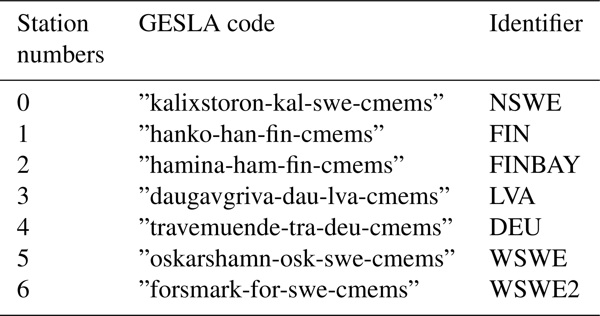
Table A2Variables from the ERA5 dataset used as predictors. The description of the data is taken from the parameter database of the official ECMWF website.
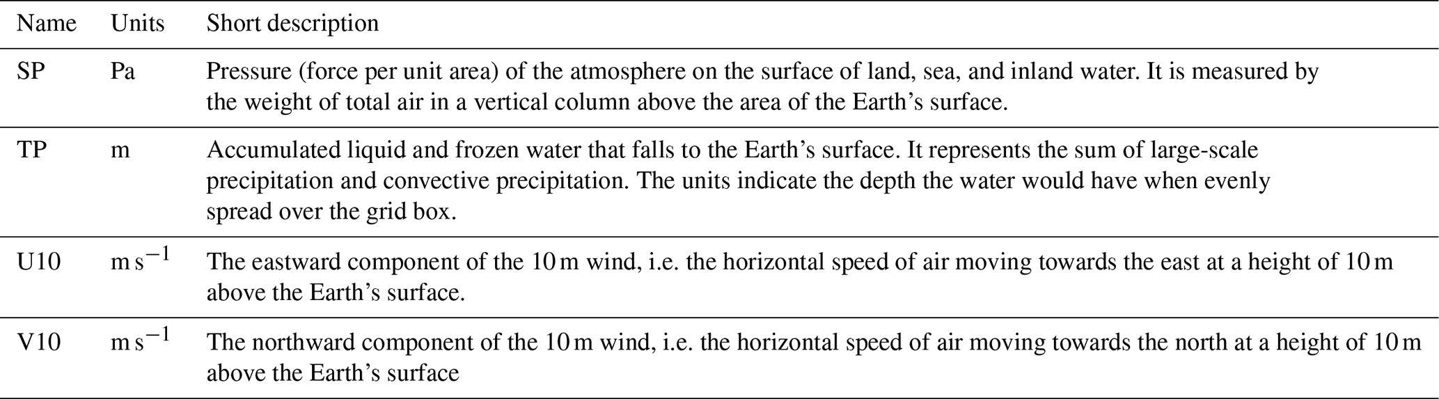
Table A3Parameters used to find optimal hyperparameters of the random forest. When multiple values are given, the optimizer chooses the best combination amongst those.
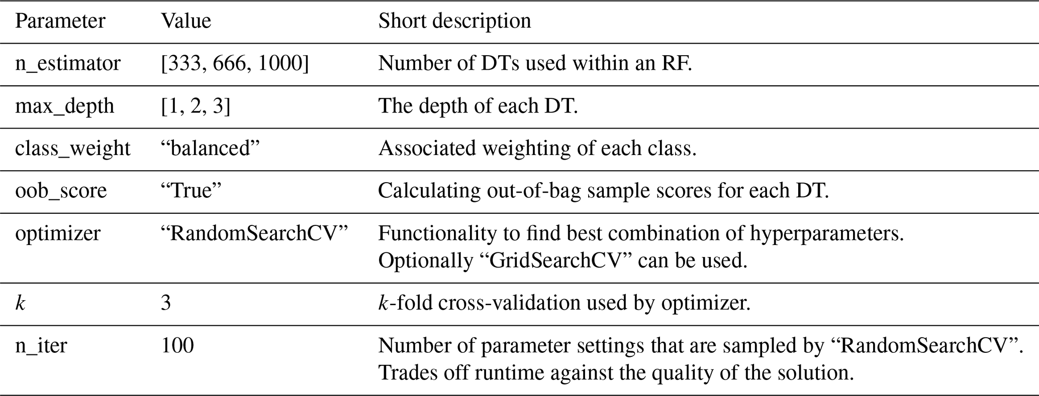
Table A4Parameters and time lags used for experiment A. All predictors are used in isolation; no combinations are used.
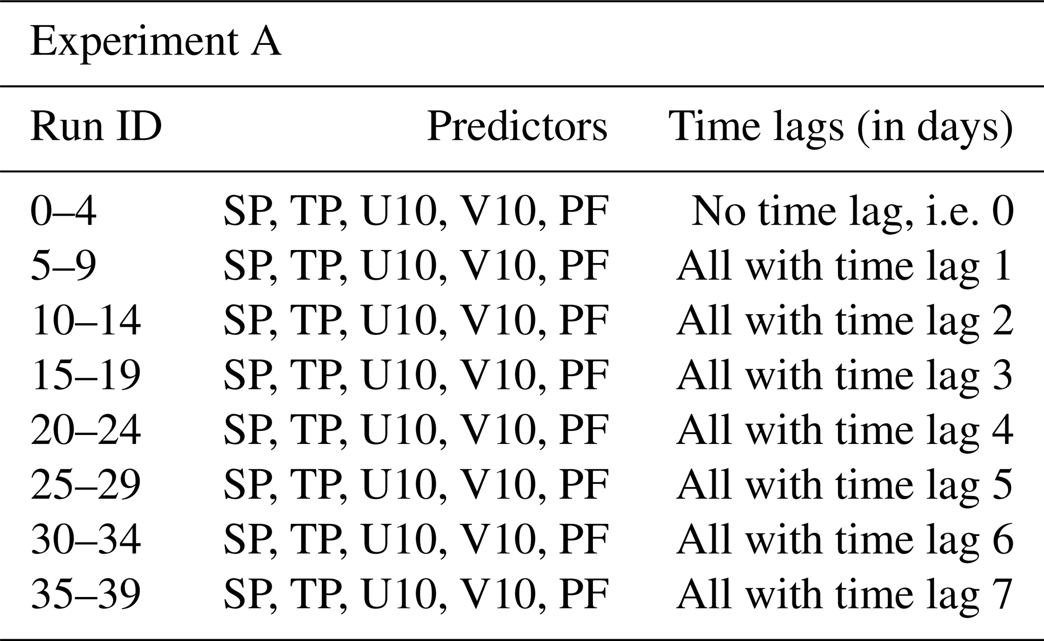
Table A5Parameters and time lags used for experiment B. Parentheses indicate that predictors are used in combination.
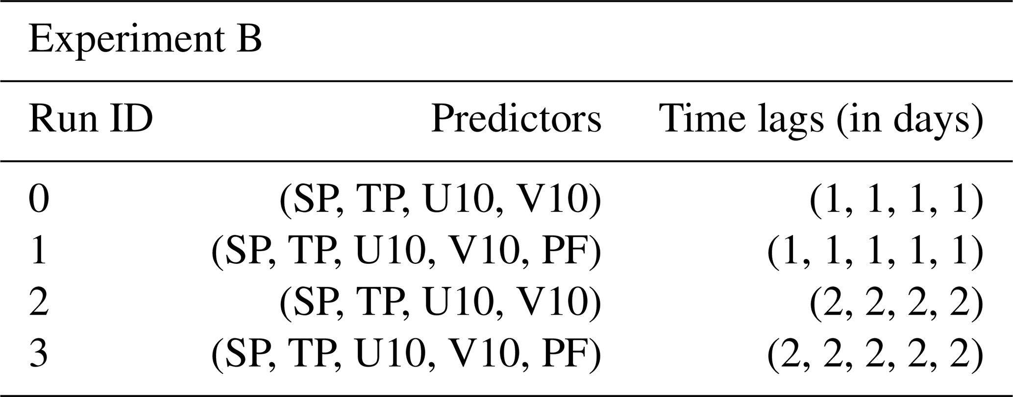
Table A6Parameters and time lags used for experiment C. Parentheses indicate that predictors are used in combination.
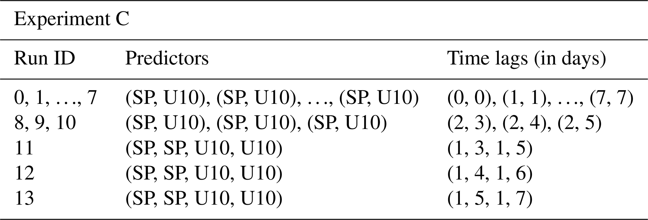
Table A7Parameters and time lags used for experiment D. Parentheses indicate that predictors are used in combination.
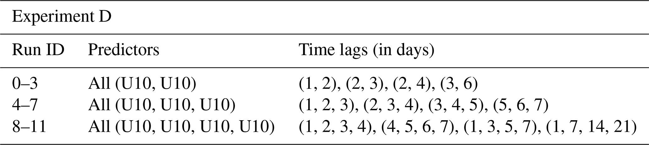
Table A8Parameters and time lags used for experiment E. Parentheses indicate that predictors are used in combination.
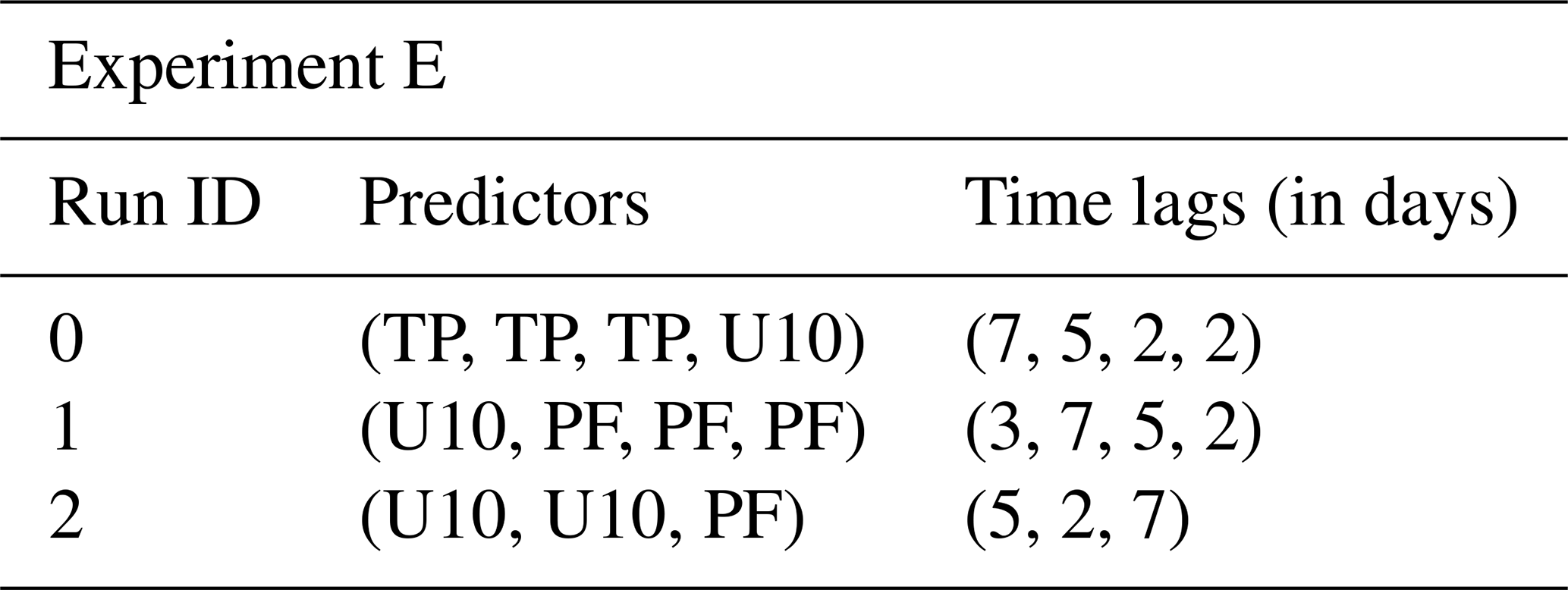
Table A9Parameters and time lags used for experiment F. Parentheses indicate that predictors are used in combination.
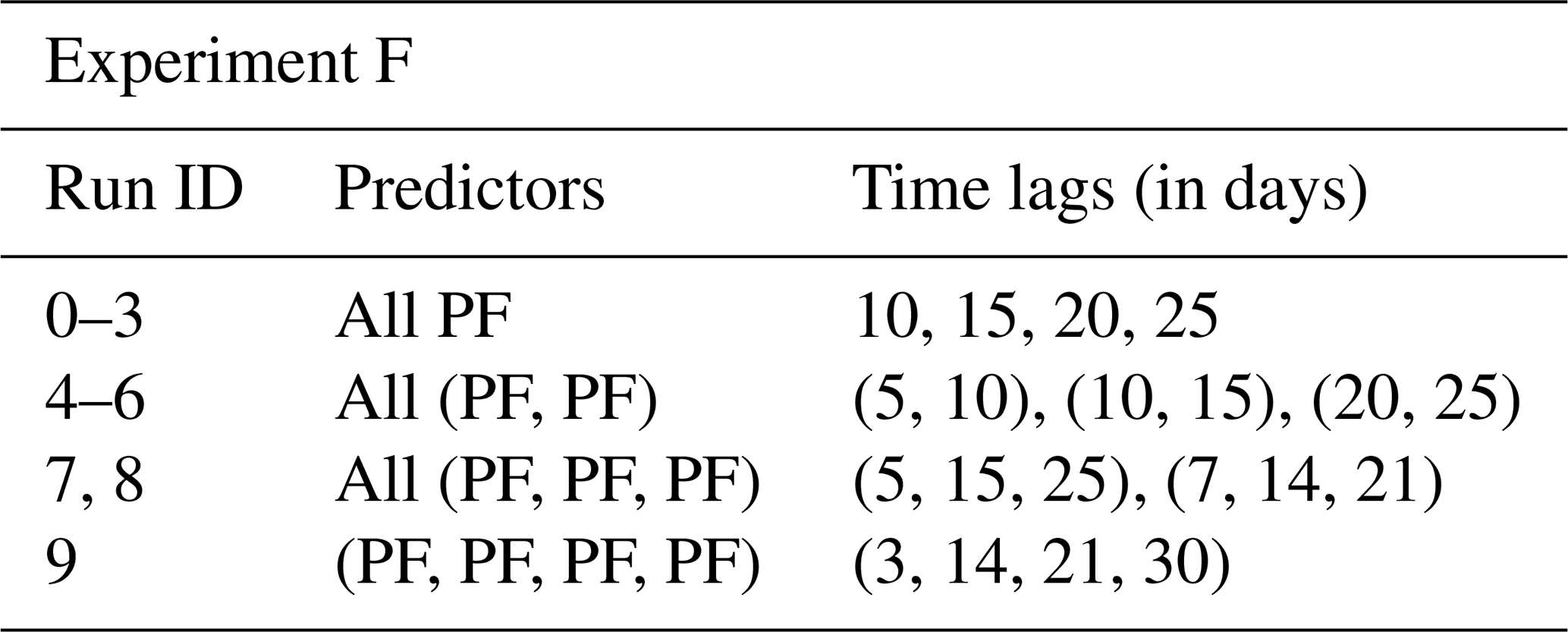
The code is available at https://doi.org/10.5281/zenodo.7409633 (Bellinghausen, 2022). The ERA5 data are publicly available at https://doi.org/10.21957/tkic6g3wm (Hersbach et al., 2018). The GESLA data are available at https://gesla787883612.wordpress.com (GESLA, 2024).
All authors contributed to the development of the original research goal and the analysis and discussion of the results. KB coded the software, carried out the data analysis, and drafted the initial versions of the paper. BH and EZ contributed to the later and final versions of the paper.
The contact author has declared that none of the authors has any competing interests.
Publisher's note: Copernicus Publications remains neutral with regard to jurisdictional claims made in the text, published maps, institutional affiliations, or any other geographical representation in this paper. While Copernicus Publications makes every effort to include appropriate place names, the final responsibility lies with the authors.
The results contain modified Copernicus Climate Change Service information 2020. Neither the European Commission nor ECMWF is responsible for any use that may be made of the Copernicus information or data it contains.
The ERA5 data (Hersbach et al., 2018) were downloaded from the Copernicus Climate Change Service (C3S) Climate Data Store. We also thank the GESLA project (https://gesla787883612.wordpress.com/, GESLA, 2024) for making the extreme sea level datasets available for the scientific community.
The article processing charges for this open-access publication were covered by the Helmholtz-Zentrum Hereon.
This paper was edited by Maria Ana Baptista and reviewed by three anonymous referees.
Andrée, E., Drews, M., Su, J., Larsen, M. A. D., Drønen, N., and Madsen, K. S.: Simulating wind-driven extreme sea levels: Sensitivity to wind speed and direction, Weather and Climate Extremes, 36, 100422, https://doi.org/10.1016/j.wace.2022.100422, 2022. a
Bellinghausen, K.: Storm Surge Model for the Baltic Sea, Zenodo [code], https://doi.org/10.5281/zenodo.7409633, 2022. a, b
Bevacqua, E., Maraun, D., Vousdoukas, M. I., Voukouvalas, E., Vrac, M., Mentaschi, L., and Widmann, M.: Higher probability of compound flooding from precipitation and storm surge in Europe under anthropogenic climate change, Science Advances, 5, eaaw5531, https://doi.org/10.1126/sciadv.aaw5531, 2019. a
Breiman, L.: Random Forests, Mach. Learn., 45, 5–32, https://doi.org/10.1023/A:1010933404324, 2001. a
Bruneau, N., Polton, J., Williams, J., and Holt, J.: Estimation of global coastal sea level extremes using neural networks, Environ. Res. Lett., 15, 074030, https://doi.org/10.1088/1748-9326/ab89d6, 2020. a, b, c, d, e, f
Chen, D. and Omstedt, A.: Climate-induced variability of sea level in Stockholm: Influence of air temperature and atmospheric circulation, Adv. Atmos. Sci., 22, 655–664, https://doi.org/10.1007/BF02918709, 2005. a
Eakins, B. W. and Sharman, G. F.: Volumes of the World's Oceans from ETOPO1, U.S. Department of Commerce, https://www.ngdc.noaa.gov/mgg/global/etopo1_ocean_volumes.html (last access: 12 July 2024), 2010. a
Field, C. B., Barros, V., Stocker, T. F., and Dahe, Q. (Eds.): Managing the Risks of Extreme Events and Disasters to Advance Climate Change Adaptation: Special Report of the Intergovernmental Panel on Climate Change, Cambridge University Press, Cambridge, https://doi.org/10.1017/CBO9781139177245, ISBN 978-1-139-17724-5, 2012. a
Géron, A.: Hands-On Machine Learning with Scikit-Learn and TensorFlow, O'Reilly Media, Inc, 564 pp., ISBN: 978-1-491-96229-9, 2017. a
GESLA (Global Extreme Sea Level Analysis): https://gesla787883612.wordpress.com, last access: 3 November 2024. a, b
Gönnert, G. and Sossidi, K.: A new approach to calculate extreme storm surges: analysing the interaction of storm surge components, WIT Trans. Ecol. Envir., 149, 139–150, https://doi.org/10.2495/CP110121, 2011. a
Gönnert, G., Dube, S. K., Murty, T., and Siefert, W.: Die Küste, 63 Global Storm Surges, Boyens Medien GmbH & Co. KG, Heide i. Holstein, ISBN 978-3-8042-1054-7, 2001. a, b, c, d, e, f
Guillory, A.: ERA5, ECMWF, https://www.ecmwf.int/en/forecasts/datasets/reanalysis-datasets/era5 (last access: 3 November 2024), 2017. a
Haigh, I. D., Marcos, M., Talke, S. A., Woodworth, P. L., Hunter, J. R., Hague, B. S., Arns, A., Bradshaw, E., and Thompson, P.: GESLA Version 3: A major update to the global higher-frequency sea-level dataset, Geosci. Data J., 10, 293–314, https://doi.org/10.1002/gdj3.174, 2021. a, b, c
Harris, D. L.: The equivalence between certain statistical prediction methods and linearized dynamical methods, Mon. Weather Rev., 90, 331–340, https://doi.org/10.1175/1520-0493(1962)090<0331:TEBCSP>2.0.CO;2, 1962. a
Harris, D. L.: Characteristics of the Hurricane Storm Surge, Technical Paper no. 48, 145 pp., U.S. Department of Commerce, U.S. Weather Bureau, https://www.weather.gov/media/owp/oh/hdsc/docs/TP48.pdf (last access: 23 December 2021), 1963. a, b, c, d
Hersbach, H., de Rosnay, P., Bell, B., Schepers, D., Simmons, A., Soci, C., Abdalla, S., Alonso-Balmaseda, M., Balsamo, G., Bechtold, P., Berrisford, P., Bidlot, J.-R., de Boisséson, E., Bonavita, M., Browne, P., Buizza, R., Dahlgren, P., Dee, D., Dragani, R., Diamantakis, M., Flemming, J., Forbes, R., Geer, A., Haiden, T., Hólm, E., Haimberger, L., Hogan, R., Horányi, A., Janiskova, M., Laloyaux, P., Lopez, P., Munoz-Sabater, J., Peubey, C., Radu, R., Richardson, D., Thépaut, J.-N., Vitart, F., Yang, X., Zsótér, E., and Zuo, H.: Operational global reanalysis: progress, future directions and synergies with NWP, ECMWF, ERA Report no. 27, https://doi.org/10.21957/tkic6g3wm, 2018. a
Hersbach, H., Bell, B., Berrisford, P., Hirahara, S., Horányi, A., Muñoz-Sabater, J., Nicolas, J., Peubey, C., Radu, R., Schepers, D., Simmons, A., Soci, C., Abdalla, S., Abellan, X., Balsamo, G., Bechtold, P., Biavati, G., Bidlot, J., Bonavita, M., De Chiara, G., Dahlgren, P., Dee, D., Diamantakis, M., Dragani, R., Flemming, J., Forbes, R., Fuentes, M., Geer, A., Haimberger, L., Healy, S., Hogan, R. J., Hólm, E., Janisková, M., Keeley, S., Laloyaux, P., Lopez, P., Lupu, C., Radnoti, G., de Rosnay, P., Rozum, I., Vamborg, F., Villaume, S., and Thépaut, Jean-N.: The ERA5 global reanalysis, Q. J. Roy. Meteorol. Soc., 146, 1999–2049, 2020. a
Holfort, J., Wisniewski, B., Lydeikaite, Z., Kowalewska-Kalkowska, H., Wolski, T., Boman, H., Hammarklint, T., Giza, A., and Grabbi-Kaiv, S.: Extreme sea levels at selected stations on the Baltic Sea coast, Oceanologia, 56, 259–290, https://doi.org/10.5697/oc.56-2.259, 2014. a, b
Hünicke, B. and Zorita, E.: Influence of temperature and precipitation on decadal Baltic Sea level variations in the 20th century, Tellus A, 58, 141–153, https://doi.org/10.1111/j.1600-0870.2006.00157.x, 2006. a
Hünicke, B., Zorita, E., Soomere, T., Madsen, K. S., Johansson, M., and Suursaar, Ü.: Recent Change – Sea Level and Wind Waves, in: Second Assessment of Climate Change for the Baltic Sea Basin, edited by: The BACC II Author Team, Regional Climate Studies, Springer International Publishing, Cham, 155–185, https://doi.org/10.1007/978-3-319-16006-1_9, ISBN 978-3-319-16006-1, 2015. a, b, c
Janssen, F., Schrum, C., Hübner, U., and Backhaus, J.: Uncertainty analysis of a decadal simulation with a regional ocean model for the North Sea and Baltic Sea, Clim. Res., 18, 55–62, https://doi.org/10.3354/cr018055, 2001. a
Leppäranta, M. and Myrberg, K.: Physical Oceanography of the Baltic Sea, in: Springer Praxis books geophysical sciences, Springer, Berlin Heidelberg, ISBN 978-3-540-79702-9, 2009. a, b, c, d, e
Mohrholz, V.: Major Baltic Inflow Statistics – Revised, 5, 384, https://doi.org/10.3389/fmars.2018.00384, 2018. a
Mudersbach, C. and Jensen, J.: Küstenschutz an der Deutschen Ostseeküste – Zur Ermittlung von Eintrittswahrscheinlichkeiten extremer Sturmflutwasserstände, 5, 10 pp., https://doi.org/10.3243/kwe2010.03.003, 2010. a, b, c
Muis, S., Verlaan, M., Winsemius, H. C., Aerts, J. C. J. H., and Ward, P. J.: A global reanalysis of storm surges and extreme sea levels, Nat. Commun., 7, 11969, https://doi.org/10.1038/ncomms11969, 2016. a, b, c, d, e, f, g, h
Müller, A. C.: Introduction to Machine Learning with Python, O’Reilly Media, Inc., USA, 392 pp., ISBN: 978-1-449-36941-5, 2017. a, b, c, d
Rutgersson, A., Kjellström, E., Haapala, J., Stendel, M., Danilovich, I., Drews, M., Jylhä, K., Kujala, P., Larsén, X. G., Halsnæs, K., Lehtonen, I., Luomaranta, A., Nilsson, E., Olsson, T., Särkkä, J., Tuomi, L., and Wasmund, N.: Natural hazards and extreme events in the Baltic Sea region, Earth Syst. Dynam., 13, 251–301, https://doi.org/10.5194/esd-13-251-2022, 2022. a, b, c, d, e
Sztobryn, M.: Forecast of storm surge by means of artificial neural network, J. Sea Res., 49, 317–322, https://doi.org/10.1016/S1385-1101(03)00024-8, 2003. a, b, c
Tadesse, M., Wahl, T., and Cid, A.: Data-Driven Modeling of Global Storm Surges, Frontiers in Marine Science, 7, 260, https://doi.org/10.3389/fmars.2020.00260, 2020. a, b
Tiggeloven, T., Couasnon, A., van Straaten, C., Muis, S., and Ward, P. J.: Exploring deep learning capabilities for surge predictions in coastal areas, Scientific Reports, 11, 17224, https://doi.org/10.1038/s41598-021-96674-0, 2021. a, b, c
Tyralis, H., Papacharalampous, G., and Langousis, A.: A Brief Review of Random Forests for Water Scientists and Practitioners and Their Recent History in Water Resources, Water, 11, 910, https://doi.org/10.3390/w11050910, 2019. a, b
von Storch, H.: Storm Surges: Phenomena, Forecasting and Scenarios of Change, Proc. IUTAM, 10, 356–362, https://doi.org/10.1016/j.piutam.2014.01.030, 2014. a
Vousdoukas, M. I., Voukouvalas, E., Annunziato, A., Giardino, A., and Feyen, L.: Projections of extreme storm surge levels along Europe, Clim. Dynam., 47, 3171–3190, https://doi.org/10.1007/s00382-016-3019-5, 2016. a
Weisse, D. R.: Klimatologie der Ostseewasserstände: Eine Rekonstruktion von 1948 bis 2011, p. 132, https://ediss.sub.uni-hamburg.de/handle/ediss/5561 (last access: 14 January 2022), 2014. a, b, c, d, e, f, g
Weisse, R. and Hünicke, B.: Baltic Sea Level: Past, Present, and Future, in: Oxford Research Encyclopedia of Climate Science, Oxford University Press, https://doi.org/10.1093/acrefore/9780190228620.013.693, ISBN 978-0-19-022862-0, 2019. a, b, c, d, e
Weisse, R. and von Storch, H.: Marine Climate and Climate Change, Springer Berlin Heidelberg, Berlin, Heidelberg, https://doi.org/10.1007/978-3-540-68491-6, ISBN 978-3-540-25316-7, 978-3-540-68491-6, 2010. a, b, c, d, e, f
Weisse, R. and Weidemann, H.: Baltic Sea extreme sea levels 1948-2011: Contributions from atmospheric forcing, Proc. IUTAM, 25, 65–69, https://doi.org/10.1016/j.piutam.2017.09.010, 2017. a
Wiśniewski, B. and Wolski, T.: Physical aspects of extreme storm surges and falls on the Polish coast, Oceanologia, 53, 373–390, https://doi.org/10.5697/oc.53-1-TI.373, 2011. a
WMO: Guide to storm surge forecasting, WMO, Geneva, oCLC: 1075529493, ISBN 978-92-63-11076-3, 2011. a, b, c, d, e
Wolski, T. and Wiśniewski, B.: Geographical diversity in the occurrence of extreme sea levels on the coasts of the Baltic Sea, J. Sea Res., 159, 101890, https://doi.org/10.1016/j.seares.2020.101890, 2020. a, b, c
Wolski, T. and Wiśniewski, B.: Characteristics and Long-Term Variability of Occurrences of Storm Surges in the Baltic Sea, Atmosphere, 12, 1679, https://doi.org/10.3390/atmos12121679, 2021. a, b, c, d, e, f, g, h, i, j, k
Woodworth, P. L., Hunter, J. R., Marcos, M., Caldwell, P., Menéndez, M., and Haigh, I.: Towards a global higher-frequency sea level dataset, Geosci. Data J., 3, 50–59, https://doi.org/10.1002/gdj3.42, 2016. a