Characteristics and mechanisms of near-surface negative atmospheric electric field anomalies preceding the 5 September 2022, M_s 6.8 Luding earthquake in China

A magnitude 6.8 strike-slip earthquake (EQ) struck Luding, Sichuan Province, China, on 5 September 2022, resulting in significant damage to nearby Ganzi Prefecture and the city of Ya'an. In this research, the near-surface atmospheric electric field (AEF) recorded at four sites 15 d before the Luding EQ was analyzed and differentiated, and multisource auxiliary data including precipitation, cloud base height, and low cloud cover were used at the same time. Nine possible seismic AEF anomalies at four sites were obtained preliminarily. Accordingly, microwave brightness temperature (MBT) data, which are very sensitive to the surface dielectrics and are closely related to the air ionization, together with surface soil moisture, lithology, and a 3D-simulated crustal stress field, were jointly analyzed to confirm the seismic relations of the obtained negative AEF anomalies. The geophysical environment for crustal high-stress concentration, positive charge carrier transfer, and surface accumulation was demonstrated to exist and to meet the conditions necessary to generate local negative AEF anomalies. Furthermore, to deal with the spatial disparities in sites and regions with potential atmospheric ionization, near-surface wind field data were employed to scrutinize the reliability of the AEF anomalies by comprehensively analyzing the spatial relationships among surface charges accumulation areas, wind direction and speed, and the AEF sites. Finally, four negative AEF anomalies were deemed to be closely related to the Luding EQ, and the remaining five possible anomalies were ruled out. A possible mechanism of negative AEF anomalies before the Luding EQ is proposed: positive charge carriers were generated from the underground high-stress concentration areas and then transferred to and accumulated on the ground surface to ionize the surface air, thus disturbing the AEF above the ground. This study presents a method for identifying and analyzing seismic AEF anomalies and is also beneficial for the examination of the pre-earthquake coupling process between the coversphere and the atmosphere.

1 Introduction

In nature, the global atmospheric electric circuit (GEC) is driven by global thunderstorm activity and large-scale ion separation in charged cloud (Rycroft et al., 2000). In the background of the GEC, a direct current (DC) atmospheric electric field with an amplitude of around 130 V m⁻¹ is always present in undisturbed fair-weather areas (Sun,1987). This electric field, also known as the fair-weather atmospheric electric field (FW-AEF), is oriented vertically downwards, which means that the atmosphere is positively charged relative to the Earth, while the Earth carries a negative charge (L. Li et al., 2022). In recent decades, some scientists have discovered that seismic activity can cause AEF anomalies with a direction opposite to FW-AEF in the seismogenic region. In 1966, Kondon (1966) found abnormal pre-earthquake (EQ) electric field signals for the first time using the field mill instrument at the Matsushiro Observatory in Japan. Based on the electric field data recorded at the Pixian and Wenjiang sites (in Chengdu, China), significant abnormal AEF phenomena were found before the 2008 M_s 8.0 Wenchuan EQ when the interference of lightning activities was excluded (Li et al., 2017). Chen et al. (2022) also observed AEF anomalies before the 2021 M_s 4.3 Luanzhou EQ at two sites in Baodi and Yongqing, China. By analyzing the meteorological data, the anomalous signal monitored at Baodi station was found to have been influenced by a combination of transit clouds and geological activity, while the bay-type persistent electric field anomaly monitored at Yongqing station was considered a possible AEF precursor of the EQ.

At present, there are three accepted mechanisms for AEF anomalies before EQs. Firstly, seismic-related anomalies in radon emanation can be linked to pre-seismic electromagnetic phenomena such as large changes in small ion concentration and AEF (Omori et al., 2007). In a recent study (Jin et al., 2020), the AEF reduction before the Wenchuan EQ was interpreted from the perspective of the rapid changing of radon concentration as the mainshock approached. Besides this, by combining the time series and dynamic periodogram of AEF anomalies from 6 h before to 6 h after the EQ, Hobara et al. (2022) attributed the phenomenon to the internal gravity waves generated near the epicenter passing through the AEF site, which changed the space charge density in the surface layer of the atmosphere. In addition, during an experimental study Freund (2000, 2010) and Freund et al. (2007) found that stress-activated carriers named positive holes (p-holes) activated in igneous and metamorphic rocks are able to transfer along stress gradients and accumulate on the rock surface in unstressed areas or even on the ground surface covered by sand. When the p-holes arrive at the air–ground interface, a positive potential can be produced and air particles here are able to be ionized so as to change the near-surface AEF when the positive potential reaches a high level (Freund, 2013). Meanwhile, the accumulation of p-holes on the ground surface is also believed to reduce the surface microwave dielectric constant and enhance regional microwave radiation (Mao et al., 2020; Qi et al., 2021a, b).

Other researchers have also proposed different opinions regarding the pre-EQ AEF anomalies observed at ground sites. Based on the statistical analysis of 103 pre-EQ bay-type AEF anomalies in the Kamchatka region, Smirnov (2019) found that the duration and magnitude of AEF anomalies at the hour-scale did not depend on either the magnitude of the EQ or the distance to the epicenter, while those at the day-scale were related to the magnitude of the EQ. Hao (1988) analyzed the AEF at the three stations in Baijiatong, Baodi, and Beidaihe for several seismic events which happened in and around Beijing from 1977 to 1986 and found that there were negative anomalies of AEF variation evident before the EQs, decaying significantly with the distance to the epicenter and only associated with nearby EQs but not far, strong EQs. However, most of the research was based on statistical judgements and has not yet been integrated with the regional geological conditions of seismogenic zones or the local crustal stress-field alteration (CSFA), which is crucial to understanding whether charges from the stressed rock mass of Earth's crust can ionize the near-surface atmosphere.

It is well known that the atmospheric vertical electric field acts as a bridge connecting the surface charges and atmospheric particle concentration. The current consensus is that the increased concentration of atmospheric ions at the ground–air interface leads to the formation of additional vertical electric fields, which further transport ions from the lower atmosphere to the upper atmosphere, ultimately causing atmospheric anomalies. In our recent research, the multiparameter seismic anomalies before the 2015 Nepal EQ sequence were analyzed systematically (Wu et al., 2023) by referring to the lithosphere–coversphere–atmosphere (LCA) coupling paradigm (Wu and Liu, 2009; Wu et al., 2012) and lithosphere–coversphere–atmosphere–ionosphere (LCAI) coupling paradigm (Qin et al., 2013). However, due to a lack of AEF observations before and during the two major EQs, the abnormal changes in atmospheric parameters, such as aerosols and humidity, cannot be well-linked to the changes in parameters of the ground surface, such as microwave brightness temperature (MBT). Thus, the coupling process between the coversphere and atmosphere was not presented perfectly. Fortunately, in the seismogenic zone of the Luding EQ in 2022, the potential AEF disturbances before the EQ were recorded at four stations, which provided an excellent chance to study the abnormal features of the AEF caused by an EQ. In this study, the characteristics of pre-seismic AEF vibrations were analyzed, and the relationships between the AEF anomalies and the Luding EQ were carefully identified using multisource auxiliary data. The mechanism of the seismic AEF anomalies was discovered by analyzing surface MBT variations and the three-dimensional crustal stress distribution. Ultimately, four out of the nine potential AEF anomalies were determined to be earthquake-related.

2 Study area and data sources

2.1 Study area

The M_s 6.8 Luding EQ happened in the county of Luding, Sichuan Province, China, at 12:52 LT (local time) on 5 September 2022 (Beijing time), with its epicenter located at 29.59° N, 102.09° E and a hypocenter depth of 14.5 km (Yang et al., 2022). The EQ occurred near the southeast Moxi section of the Xianshuihe fault (XSHF), which is a left-slip fault between the Bayan Har Block and the Sichuan–Yunnan Block (Ji et al., 2020). The study area of 28–32° N, 99–106° E was selected after consideration of the Dobrovolsky formula (Dobrovolsky et al., 1979) and the geographical regions of the AEF observatories, in which the Longmenshan fault (LMSF), the Anninghe fault (ANHF), the Longquanshan fault (LQSF), and the XSHF are located. Among these faults, the LMSF was the source of two significant earthquakes in the last few decades: the Lushan EQ in 2013 and the Wenchuan EQ in 2008, the latter having had a catastrophic impact on human lives. The AEF data used in this study were from four observatories called GAR, GUZ, SWG, and LES. The first three are located near the XSHF, while LES is located east of the southwest section of the LQSF. Figure 1 shows a complete overview of the study area.

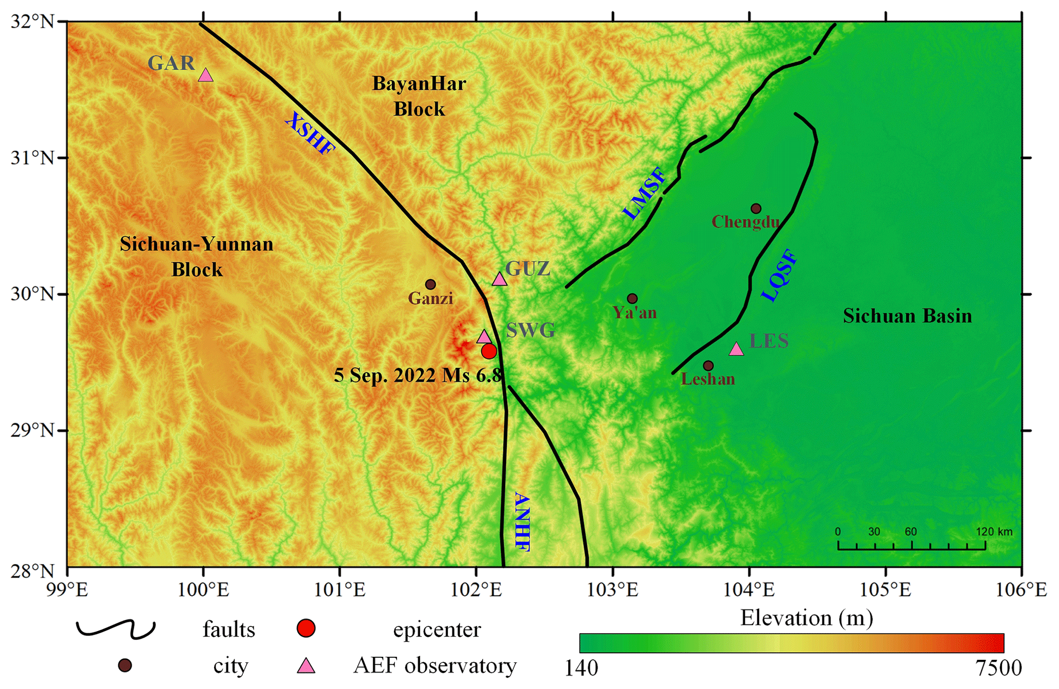
Figure 1 Distribution of the AEF observatories and topography of the study area. The background image is the digital elevation derived from Shuttle Radar Topography Mission (SRTM) datasets.

2.2 Data sources

2.2.1 Atmospheric electric field observatories

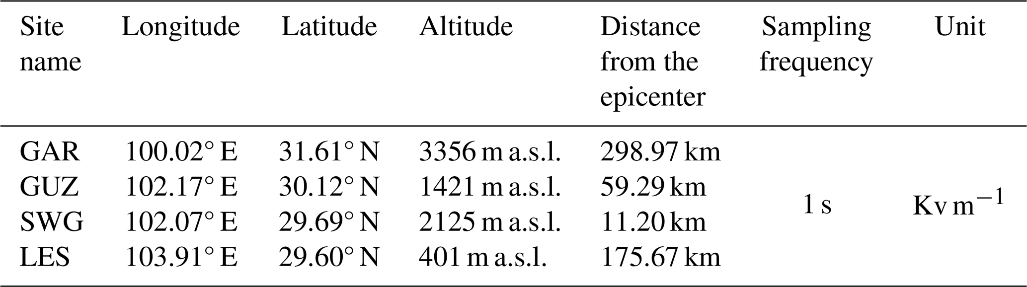
GAR, GUZ, and SWG were deployed by National Space Science Centre of Chinese Academy of Sciences (CAS) with EFM-100 electric field monitoring instruments (L. Li et al., 2022). This type of instrument is independently developed by CAS, with a range of ±50 kV m⁻¹, a relative accuracy of ±1 %, and a resolution of 10 V m⁻¹. The LES Campbell Scientific (CS) 110 instrument, which has a range of ±21.2 kV m⁻¹, a relative accuracy of ±1 %, and a resolution of 3 V m⁻¹, was deployed by China University of Geosciences (Wuhan) (Chen et al., 2021). Specific information regarding these AEF observatories is shown in Table 1. GAR is located in a highland area in the southeast of Ganzi Prefecture at an altitude of 3356 m a.s.l. (meters above sea level). GUZ is located in Guzan, Kangding, in a saddle with the Dadu River flowing through it on the east side, at an altitude of 1421 m a.s.l. SWG is located in a valley in Yanzigou, in the county of Luding, at an altitude of 2125 m a.s.l. LES is located in Leshan in the plains area, with flat terrain around it and with an altitude of 401 m a.s.l.

Table 1 Key information regarding the AEF observatories.

The intensity of AEF is measured according to the principle that a conductor can generate an induced charge in an electric field. If a metallic conductor with surface area S_C is exposed to an electrostatic field of electric field strength E, the charge density ϕ of the induced charge generated on its surface can be expressed as

$$\begin{array}{}\text{(1)}& \mathit{\varphi }={\mathit{\epsilon }}_{\mathrm{0}}KE,\end{array}$$

where ε₀ represents the air dielectric constant and K is the electric field distortion coefficient. The induced charge Q can be expressed as

$$\begin{array}{}\text{(2)}& {\displaystyle }& {\displaystyle }Q=\mathit{\varphi }{S}_{\mathrm{C}}={\mathit{\epsilon }}_{\mathrm{0}}KE{S}_{\mathrm{C}},\text{(3)}& {\displaystyle }& {\displaystyle }E={\displaystyle \frac{Q}{{\mathit{\epsilon }}_{\mathrm{0}}K{S}_{\mathrm{C}}}}.\end{array}$$

Consequently, by measuring the induced charge, the strength of the AEF can be determined. An electric current is generated when a metallic conductor is connected to the ground. If the conductor generates a continuously varying induced charge, the measured intensity of the induced current can be expressed as

$$\begin{array}{}\text{(4)}& I={\displaystyle \frac{\mathrm{d}Q}{\mathrm{d}t}}.\end{array}$$

The AEF meter sensor uses a moving piece and a stator to produce a continuously changing induced charge. As the moving piece begins to rotate, the stator is periodically exposed to the electric field or shielded under the moving piece, and the two-stage circuit receives a current signal of equal magnitude and opposite direction (Ji, 2022). Therefore, E can be deduced by measuring the intensity of the induced current

$$\begin{array}{}\text{(5)}& E={\displaystyle \frac{Q}{{\mathit{\epsilon }}_{\mathrm{0}}K{S}_{\mathrm{C}}}}={\displaystyle \frac{\int \mathrm{Idt}}{{\mathit{\epsilon }}_{\mathrm{0}}K{S}_{\mathrm{C}}}}.\end{array}$$

2.2.2 Meteorological data and MBT

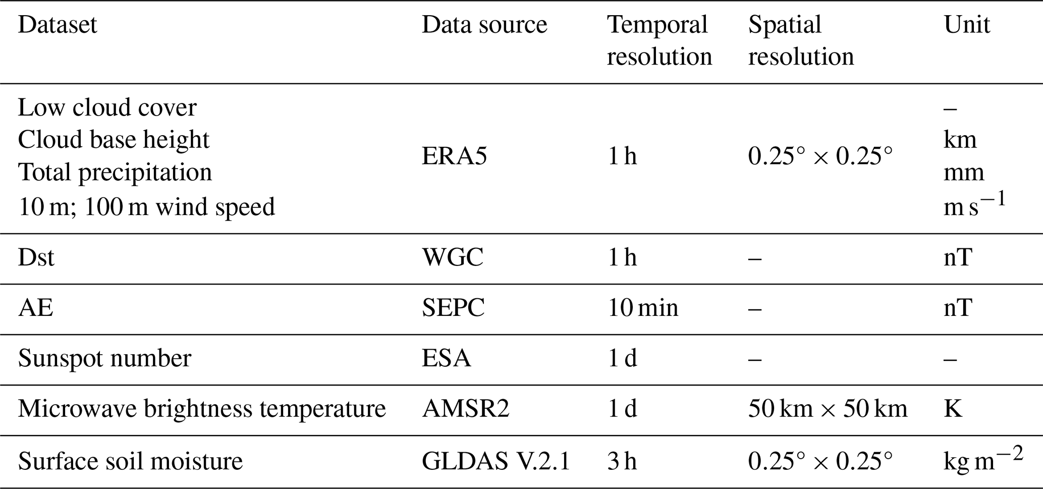
The AEF is influenced by a range of factors, including, but not limited to, meteorological conditions like clouds, rain, snow, and lightning, as well as global space weather activity such as solar activity and geomagnetic disturbances (Sun, 1987). To accurately determine if the anomalous signals are caused by an EQ, it is essential to eliminate all potential influencing factors. In this research, the meteorological data used include low cloud cover (LCC), cloud base height (CBH), total precipitation (TP), and wind field, which are from the ERA5 reanalysis dataset provided by the European Centre for Medium-Range Weather Forecasts. The dataset is a globally complete and consistent dataset formed by combining model data with global observation data using the laws of physics, which has been widely used for climatological studies. The LCC in the grid refers to the proportion of clouds that are below 2 km, CBH refers to the height of the lowest cloud base above the Earth's surface, TP is the cumulative value of liquid and frozen water falling on the Earth's surface over a period of time, and wind field includes the wind speed (WS) and direction at a height of 10 m above the ground (Hersbach et al., 2023). The space weather data used include the geomagnetic Disturbance Storm-Time Index (Dst) from the World Geomagnetic Centre (WGC), the AE index from the Space Environment Prediction Center (SEPC) (Luo et al., 2013), and the sunspot numbers (SSN) from ESA.

MBT data and surface soil moisture (SSM) data were also used to exclude local drought factors, as well as to analyze the potential accumulation of positive charge for the generation of AEF anomalies. The MBT data used are from the high-performance microwave radiometer Advanced Microwave Scanning Radiometer 2 (AMSR2) on board Global Change Observation Mission-Water (GCOM-W1), which is available at five microwave frequencies in both horizontal and vertical polarization (Imaoka et al., 2012). The UTC of MBT data has been converted to local time based on the satellite transit time. SSM data are derived from the Global Land Data Assimilation System (GLDAS) dataset, which represents a measure of moisture in the soil at a depth of 0–10 cm  b.g.s. (below ground surface) (Rodell et al., 2004). Details of all the data used are shown in Table 2.

Table 2 Multi-source data for anomaly discernment.

3 Results and analysis

3.1 Characteristics of local fair-weather AEF

To ascertain the periodic variations in AEF in the observatory, characterizing the background of FW-AEF is of great importance. Consequently, obtaining a typical AEF curve as the FW-AEF background of GEC is crucial for the identification and extraction of AEF anomalies. At present, the screening criteria for FW-AEF (Israelsson and Tammet, 2001; Harrison and Nicoll, 2018) cannot be fully standardized and need to be modified in conjunction with local topographical features, meteorological disturbances, and the geographical environment around the site. In this study, the following screening criteria were set to obtain FW-AEF: (1) no daytime rainfall, (2) low cloud cover close to zero, (3) no thunderstorms, (4) wind speed less than 8 m s⁻¹ at 10 m above the ground, and (5) no long periods of negative AEF anomalies (to exclude anthropogenic influence and other uncertain factors). Sunrise occurs between 06:41 and 06:50 LT, while sunset takes place between 19:24 and 19:30 LT in the study area. The AEF data analyzed were from 1 May to 30 September 2022 for GAR, GUZ, and SWG and from 1 August to 30 September 2022 for LES, based on the data availability. After filtering and processing the AEF data, the daily variation curves of FW-AEF for the four sites were obtained (Fig. 2).

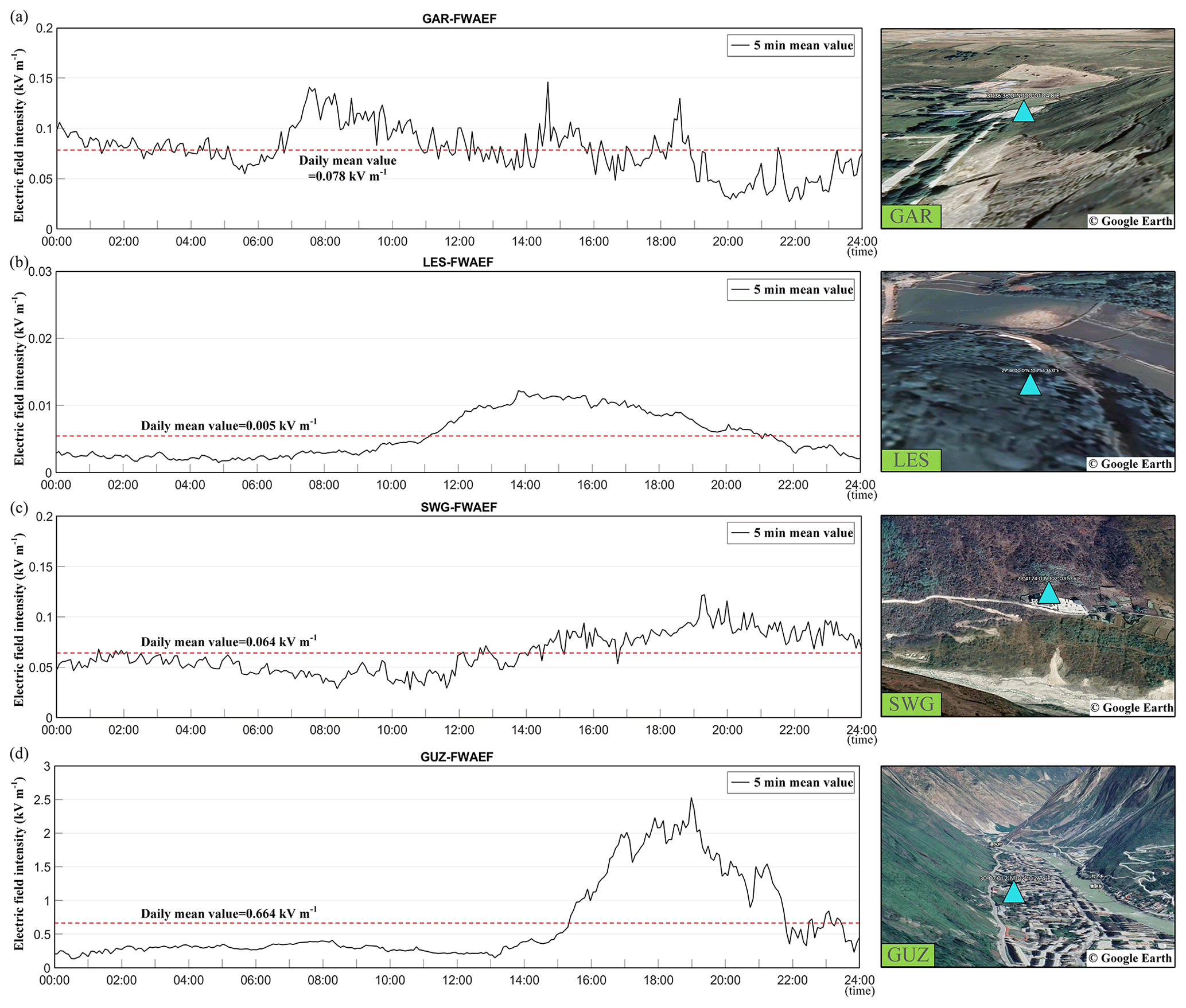
Figure 2 Daily variation in FW-AEF (left) and © Google Earth images (right) at the four sites: GAR (a), LES (b), SWG (c), and GUZ (d).

Figure 2 shows the 5 min mean curve (left) of FW-AEF and a satellite image from Google Earth (right). The AEF zero-value line is able to better identify negative AEF anomalies. Overall, the FW-AEF curve at GAR is characterized by a single peak and two valleys, which display a shallow valley of 0.023 kV m⁻¹ around 06:30 LT, then show a quick rise, and reach the peak of 0.23 kV m⁻¹ between 07:00 and 08:00 LT followed by a gradual decline. The second valley appeared between 19:00 and 20:00 LT with a low of 0.015 kV m⁻¹. The FW-AEF at LES varies more gently and shows a single-peaked pattern, which showed a peak of 0.012 kV m⁻¹ at around 14:00 LT. The AEF values of SWG and GUZ change slightly before 12:00 LT but increase gradually to a peak about 0.14 kV m⁻¹ for SWG and 2.7 kV m⁻¹ for GUZ around 19:10 LT. The FW-AEF of SWG and GUZ were both single-peaked. The peak of the FW-AEF curve of GUZ is much higher, which may be attributed to the particular topography of the river valley and the greater impact of human activity on the town.

3.2 Identification of potential seismic AEF anomalies

Lightning, haze, meteorological events such as clouds and rain, and space weather events such as magnetic storms and solar activity are able cause changes in AEF. Global space weather events such as geomagnetic disturbances (Kleimenova et al., 2008), magnetic sub-bursts in the polar regions (Davis and Sugiura, 1966), and solar activity (Tacza et al., 2018) can also affect the AEF. Dst, AE, and SSN were utilized to represent the intensity of geomagnetic activity, polar magnetic storm, and solar activity, respectively. Figure 3a shows the variations in the three indices from 22 August to 5 September. According to the authors below, −50 nT < Dst < −30 nT represents weak magnetic storm activity (Loewe and Prölss, 1997), AE < 100 nT represents calm activity of the polar area magnetic substorms (Li et al., 2010), and 40 < SSN < 80 represents moderate solar activity. From 22 to 25 August, the intensity of the three activities was very weak, and AEF was not affected by space weather events during this period. Except for the period from 18:00 LT on 4 September to 06:00 LT on 5 September, all other time periods have Dst greater than −50 nT, which represents weaker magnetic storm activity in the low-latitude region in these time periods, and the effect of this type of activity on the AEF can be ignored. Since the AE showed a higher value after 27 August, the AEF anomalies in the 4 h before the EQ did not match the high AE value in time. Therefore, even if AE fluctuated, the effect on the AEF near the epicenter was very limited and unable to cause the AEF anomalies.

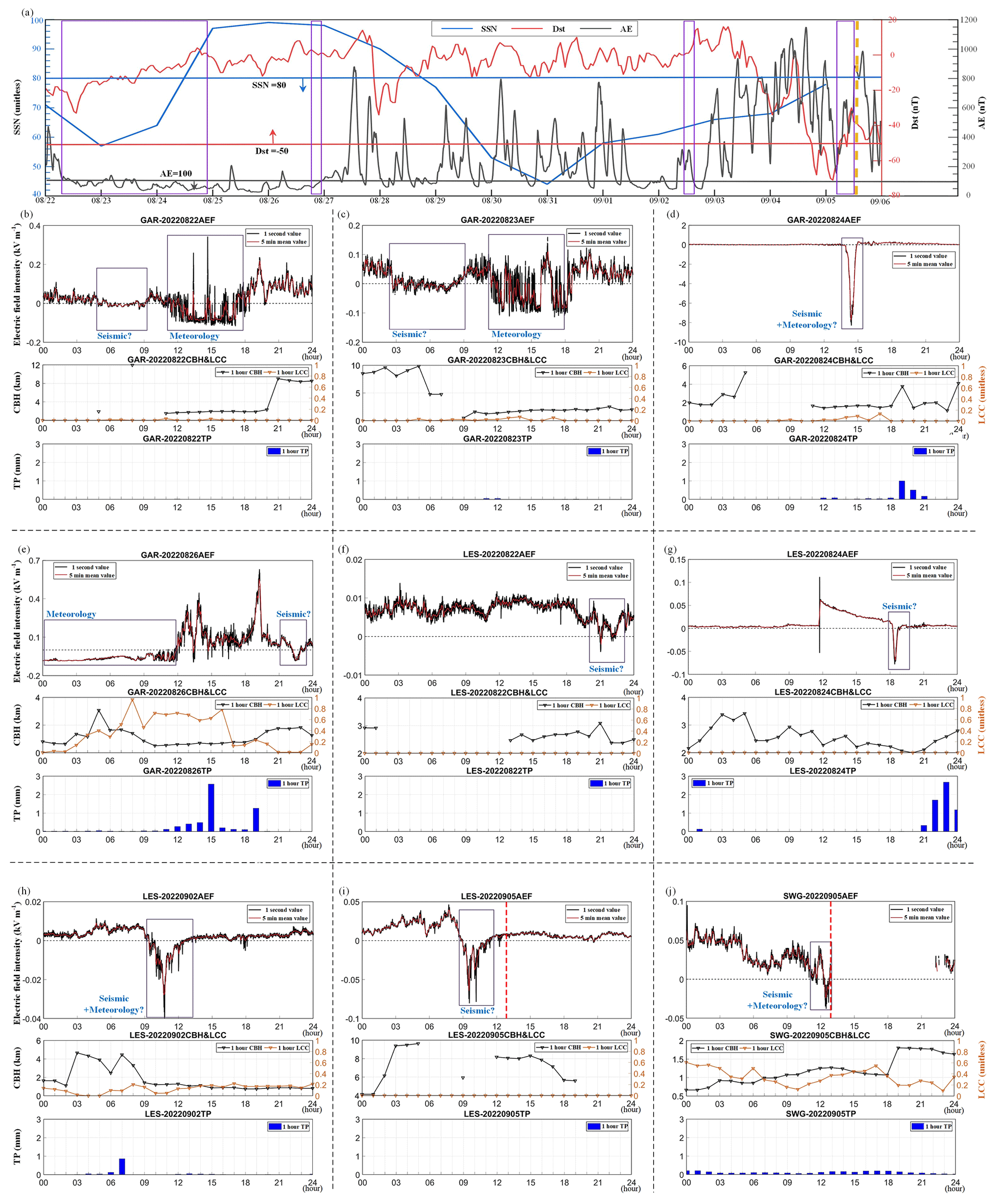
Figure 3 Changes in SSN (blue), Dst (red), and AE (grey) from 22 August to 5 September. Thick horizontal lines of different colors indicate the thresholds of geomagnetic and solar activity for quiet periods represented by the corresponding indices, where the direction of the arrows represents a weakening of activity intensity (a). Nine negative AEF anomalies possibly related to the Luding EQ and hour-by-hour meteorological parameters (including CBH, LCC, and TP) for the corresponding time periods (b–j).

In order to eliminate the effects of meteorology and space activities on the AEF, this study performed a time-series analysis of various climatological data (such as CBH, LCC, and TP) on an hourly or daily average basis. For the period of negative AEF anomalies, climatological data were examined to determine if non-seismic factors (meteorological parameters) occurred simultaneously, as depicted in Fig. 3b–j. The daily variation curves of AEF from 22 August to 5 September and the hourly results of CBH, LCC, and TP for the corresponding periods were retrieved, and nine periods of negative AEF anomalies with possible seismic activity factors were screened out from all four sites. Specifically, there were four anomalies at GAR, four anomalies at LES, and one anomaly at SWG.

At GAR, the AEF curves on 22 August and 23 August showed relatively similar patterns, with both negative AEF anomalies occurring twice during the daytime. The first AEF anomaly appeared before 09:00 LT, without low cloud cover or precipitation, which indicates that it likely had been influenced by seismic activity. The second negative anomaly appeared between 12:00 and 18:00 LT, with a small amount of precipitation at the beginning accompanied by a sudden drop in the height of the cloud base and a rise in the amount of low cloud cover, indicating that the anomaly might have been caused by the combination of clouds and precipitation. The AEF anomaly of larger amplitude appeared between 13:00 and 15:00 LT on 24 August with almost no precipitation, CBH less than 1.5 km, and LCC less than 0.1. However, the influence of TP and cloud cover was much more pronounced at this time, but the AEF did not show any negative anomaly. Hence, a mixture of meteorological and seismic activity is considered a possible cause of the negative anomaly on 24 August. Two negative AEF anomalies appeared on 26 August, from 00:00 to 12:00 LT and from 21:00 to 23:00 LT. In the period of the first AEF anomaly, there was a prolonged small amount of TP with a gradual rise in LCC and a sudden increase in TP after the negative anomaly disappeared, which means that the AEF anomaly was probably a result of persistent precipitation washing away positive ions above the ground. The second segment of the AEF showed a decreasing trend at 21:00 LT and reached a minimum value at 22:30 LT, returning to the FW-AEF level half an hour later, during which time the LCC was close to zero and there was no TP, which was basically in line with the FW-AEF conditions. Hence, the second AEF anomaly on 26 August could be attributed to seismic activity.

At LES, the AEF anomaly appeared on 22 August between 20:00 and 23:00 LT, with no precipitation, no low cloud cover, and CBH greater than 2 km throughout the day, which fully met the criteria for the FW-AEF. Precipitation and low clouds were not present during the period of the AEF anomaly occurring between 18:00 and 19:00 LT on 24 August. The negative anomalies on 2 and 5 September both appeared between 08:00 and 12:00 LT, with LCC less than 0.1 during the anomalies but with high precipitation before and slightly higher precipitation after the anomalies. There was no TP or LCC on 5 September, with CBH greater than 4 km all day. Therefore, it was determined that the negative AEF anomalies that appeared on 22 and 24 August and on 5 September might have been influenced by seismic activity, while the negative AEF anomaly that appeared on 2 September could be attributed to a mixture of meteorological and seismic activity.

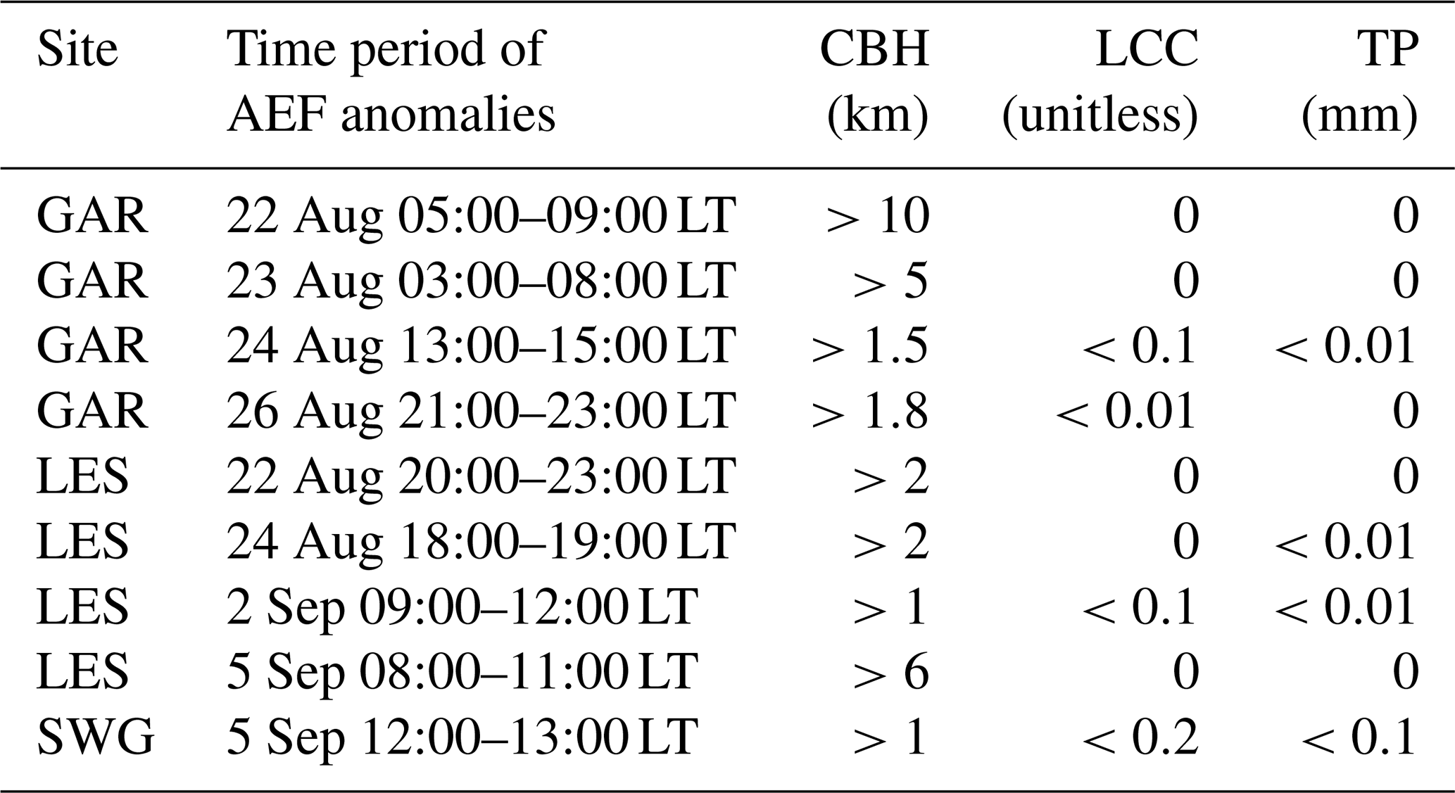
At SWG, the AEF on 5 September showed a downward trend from 04:00 LT, dropping to a negative level at around 12:15 LT, and the negative state lasted for 35 min until 12:50 LT, reaching a minimal value of −0.04 kV m⁻¹ at 12:29 LT. Due to the proximity of the site to the epicenter, the EQ triggered a power outage in the adjacent area, resulting in missing data at SWG after 12:53 LT. The site had light rain all day, with precipitation less than 0.2 mm, CBH greater than 500 m, and LCC less than 0.6. However, as compared to the FW-AEF at SWG, the decreasing trend of AEF from 04:00 to 09:00 LT coincided perfectly with the simultaneous FW-AEF changes, and there was no significant change in magnitude, so the effect of meteorological activity on AEF on 5 September was not particularly significant. In summary, the negative AEF anomaly that appeared between 12:00 and 13:00 LT could be attributed to a combination of meteorological and seismic activity. Details of each parameter related to the negative AEF anomalies are shown in Table 3.

Table 3 Details of each parameter of the anomalous AEF time periods.

4 Verification and scrutiny

The fluctuation in AEF, which is influenced by global thunderstorm activity, is primarily dependent on the concentration of near-surface atmospheric ions. Atmospheric ions exist in the air even in fair-weather conditions and contribute to the atmosphere's electrical conductivity. The concentration of atmospheric ions can be directly or indirectly altered by factors such as rainfall, low clouds, haze, and aerosols. Therefore, it is important to understand why the near-surface ion concentrations changed prior to the earthquake, in order to uncover the underlying correlation between pre-seismic AEF anomalies and the Luding earthquake.

4.1 P-hole manifestation verified by MBT, SSM, and geology

Researchers have explained the reasons for positive MBT anomalies preceding EQs from the perspective of p-hole theory (Qi et al., 2022; Ding et al., 2021), and the AEF anomaly was mentioned in the conceptual diagrams of the LCAI coupling process. Mao et al. (2020) demonstrated that the microwave dielectric constant decreases experimentally on rock surfaces under compressive loading. The pre-seismic MBT anomalies in the Qinghai–Tibet Plateau region have been extensively discussed in previous studies. Liu et al. (2023) analyzed the relationship between MBT anomalies and extensional faults. Qi et al. (2021a) discovered the positive MBT anomaly preceding the May 2008 Wenchuan EQ and explained the geological influence on the positive MBT anomaly based on p-hole theory. When p-holes are transferred to the surface, they not only change the dielectric constant but also cause air ionization near the surface. According to the research on seismic MBT anomalies in the same area as this study, MBT at a low frequency with horizontal polarization performed better (Qi et al., 2021a, 2023).

Therefore, MBT data at 10.65 GHz with H polarization were used in this study. To analyze the potential surface microwave dielectric changes caused by the seismicity, the MBT anomalies during the 15 d before the Luding EQ were obtained using a spatiotemporally weighted two-step method (STW-TSM) (Qi et al., 2020). Theoretically, MBT depends largely on the surface emissivity, which relies on the dielectric constant and the physical temperature (Ulaby et al., 1981). The surface dielectric constant increases and results in a decrease in MBT when SSM rises. Temperature changes, precipitation processes, and the rise and fall of the underground water level all lead to changes in SSM, which can also affect surface MBT. In order to identify seismic MBT anomalies, it is necessary to use SSM data to differentiate the potential MBT anomalies. In this research, SSM residuals from the surface to 10 cm underground were obtained by subtracting the average value of the same time period of the background year from the seismic year data, which was used to separate the local drought factor.

Figure 4 shows the residual MBT and residual SSM images from 22 August to 5 September 2022. Overall, the positive MBT anomalies appearing from 22 August to 1 September were mainly concentrated in the plains to the east of the LMSF, the mountainous areas to the west and northwest of the XSHF (mainly bare land), and the southeast corner of the Bayan Har block. Positive MBT anomalies gradually appeared in various areas on 22 August, with their range expanding to the maximum and their amplitude reaching 10–15 K on 25 August. Positive MBT anomalies still existed in a few areas after 28 August and generally dissipated after 2 September. The residual SSM remained at a lower value in most of the regions from 22 to 28 August, and there was also a significant increase on 30 August and a slow decline on the coseismic day. Therefore, positive MBT anomalies due to local drought factors (SSM drop) should be excluded hereinafter. Specifically, the areas of positive MBT anomalies are distinguished by different colored shapes with dashed lines in Fig. 4. The sequential positive MBT anomalies were zoned as zone I–VII, and their spatial relations to the surface lithology are shown in Fig. 5.

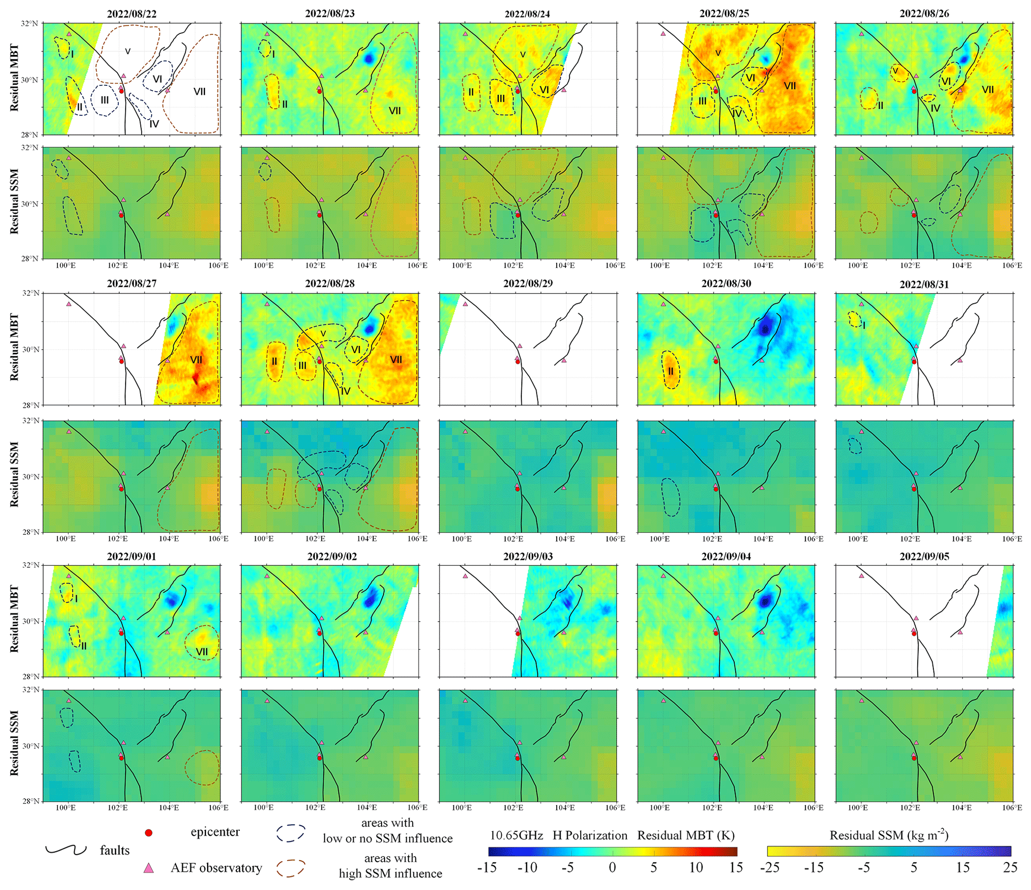
Figure 4 Residual MBT images at 10.65 GHz with H polarization and residual SSM from 22 August to 5 September. Blue shapes with dashed lines represent relatively low change or no change in SSM, while red shapes with dashed lines represent a significant drop in SSM.

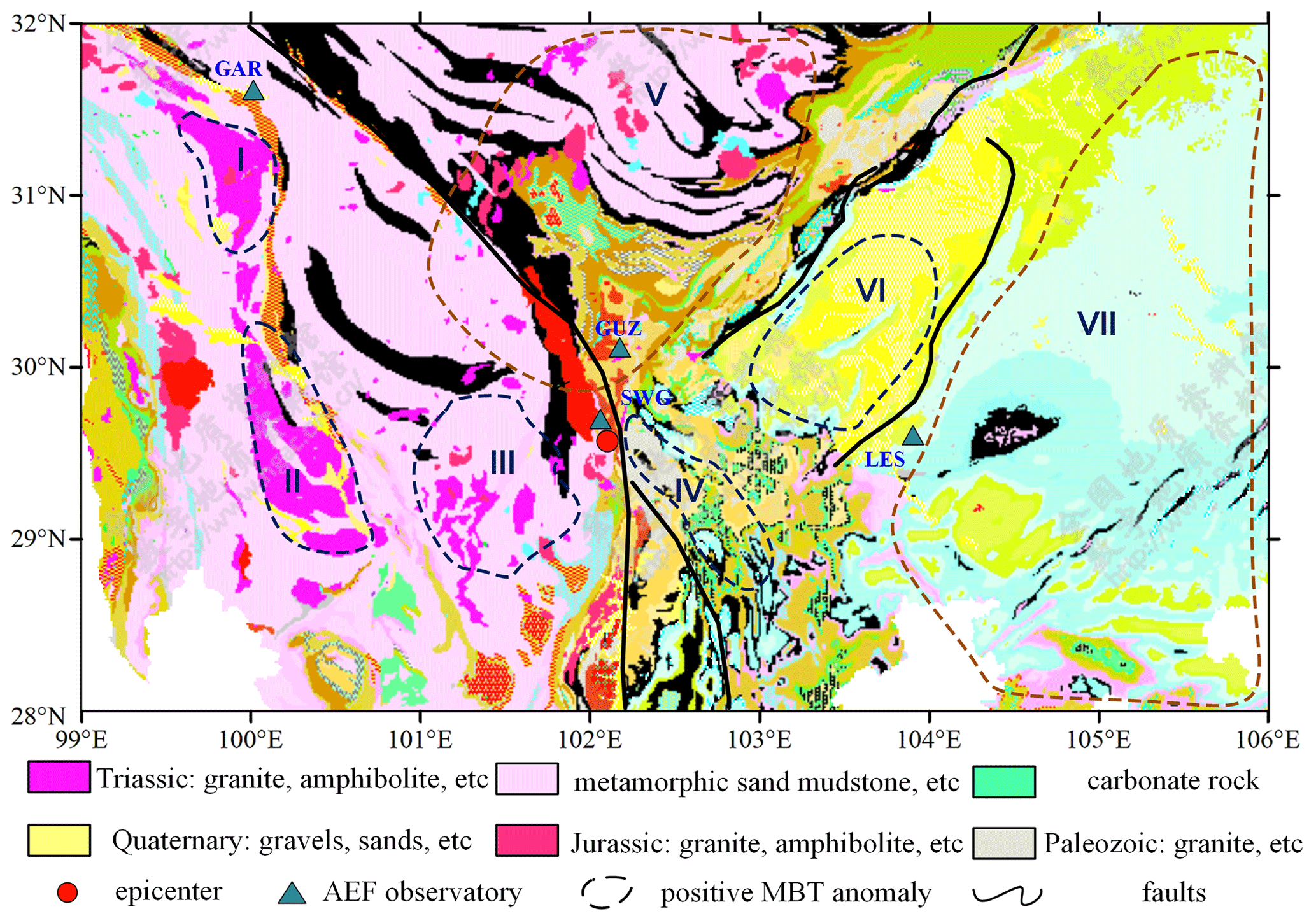
Figure 5 Distribution of surface lithology in the study area (image from the National Geological Archives).

Zone I is in the northwest corner of the study area, near the Ganzi section of the XSHF. The MBT anomaly in zone I appeared on 22 August with an amplitude of 8 K (14 d before the EQ), followed by a gradual decrease until 28 August. It appeared again on 31 August, with the positive anomaly spreading southward on 1 September and dissipating after 2 September (3 d before the EQ). SSM residuals in zone I decreased by a smaller amount than in the surrounding area from 22 to 28 August and remained almost unchanged after 31 August. The residual MBT and SSM did not conform in time to the physical process in which SSM decrease leads to the rise in MBT. Likewise, the spread of the positive MBT anomaly to the north on 28 August and the persistence of the MBT anomaly on 30 August in zone II cannot be well explained by SSM changes either.

The MBT anomalies in zone III were generally banded along the XSHF and started to appear on 23 August (13 d before the EQ), with their amplitude increasing on 24 August and basically dissipating on 26 August. The MBT anomalies appeared again on 28 August with a maximum amplitude of about 10 K then gradually weakened before the EQ. The residual SSM in zone III was low on 23 and 24 August, which was inconsistent with the amplitude increase in the MBT anomaly. A small decrease in SSM residuals appeared in zone III on 28 August, which was consistent with the appearance of the positive MBT anomaly. There was a good spatiotemporal correlation between the positive MBT anomaly and SSM decline.

Positive MBT anomalies in zone IV gradually became apparent on 24 August and became more pronounced in the north on 26 August and in the south on 28 August. The SSM residuals were in a state of low negative value from 24 to 28 August, and no significant change was detected over time. This was also the case for zone VI, where the variation in SSM was slight during the MBT anomalies from 24 to 28 August. The positive MBT anomalies in zone V mainly appeared on 24 and 25 August, with a large range of high amplitude. The SSM in zone V decreased during the same period and then SSM residuals gradually increased, which corresponded well with the positive MBT anomalies on the space scale and timescale. The same situation as occurred in zone V also happened in zone VII from 23 to 31 August.

After analyzing the spatiotemporal evolution of MBT residuals and SSM residuals in the seven zones of MBT anomalies, the appearance of positive MBT anomalies in five zones (I, II, III, IV, and VI) was thought to be related to the Luding EQ. Accordingly, the positive MBT anomalies associated with seismic activity in these five zones were further analyzed by introducing the lithology distribution map and numerical simulations of the CSFA. Figure 5 shows the surface lithology in the study area. According to p-hole theory, the production and convergence of p-holes occur in rocks with peroxy-defect (peroxy-bonded) structures, and the main carriers of peroxy-bonded defects are low-crystalline minerals including quartz and feldspar (Freund, 2002). As can be seen in Fig. 5, the lithology of zone I, II, and III is dominated by granite, metamorphic sandstone, and other rocks containing quartz and feldspar components with peroxy-defect structures. Zone VI is dominated by the Quaternary, the geological strata are relatively loose, and the major lithological features are sand and gravel consisting of granular quartz, feldspar, mica, etc. Zone IV has a more complex lithological distribution, having fewer minerals with a peroxy-defect structure than the others, and the positive MBT anomalies which appeared in zone IV were shorter in duration and relatively small in area. Therefore, we consider zones I, II, III, and VI as more prone to positive MBT anomalies following p-hole accumulation.

Gradual accumulation of unevenly distributed crustal stress is the main cause of tectonic seismicity. Based on the CRUST 2.0 crustal model and stratigraphic data (Shan et al., 2009; Y. C. Li et al., 2022), a three-dimensional (3D) stratigraphic model was constructed using the 3D finite element method to simulate the CSFA due to seismic tectonics at a timescale of 1000 years. The stratigraphic model had an east–west width of 1000 km, a north–south width of 800 km, and a depth of 83 km, and the simulated crustal stress within the study area of this research was visualized (Fig. 6). Historical EQ catalogs from 1770 to 2022 were selected to perform the seismic validation of the simulated CSFA.

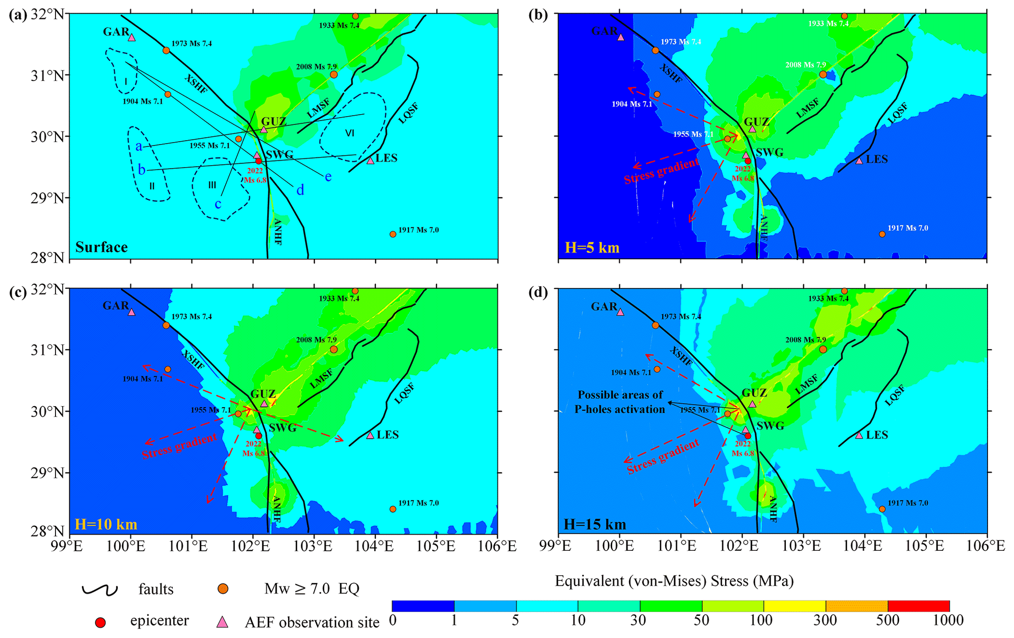
Figure 6 Spatial distribution of equivalent stress at the ground surface (a), 5 km deep (b), 10 km deep (c), and 15 km deep (d).

As shown in Fig. 6, the equivalent stress intercepted at different depths was used to show the crustal stress background. In the map of the CSFA at a depth of 15 km, crustal stress was mainly concentrated in three places, i.e., the left side of the southeast section of the XSHF, the area along the LMSF, and the right side of the ANHF. Large EQs (magnitude of 7 or higher) have occurred in all three places in history. The activated p-holes flow from the seismic source area to the upper crust in response to the direction of the maximum stress gradient (Freund et al., 2006, 2021; St-Laurent et al., 2006). Compared to the stress concentration areas at a depth of 15 km, the size of the surface stress concentration areas and the stress magnitude are weakened, indicating an overall upward stress gradient between the 15 km depth plane and the ground surface.

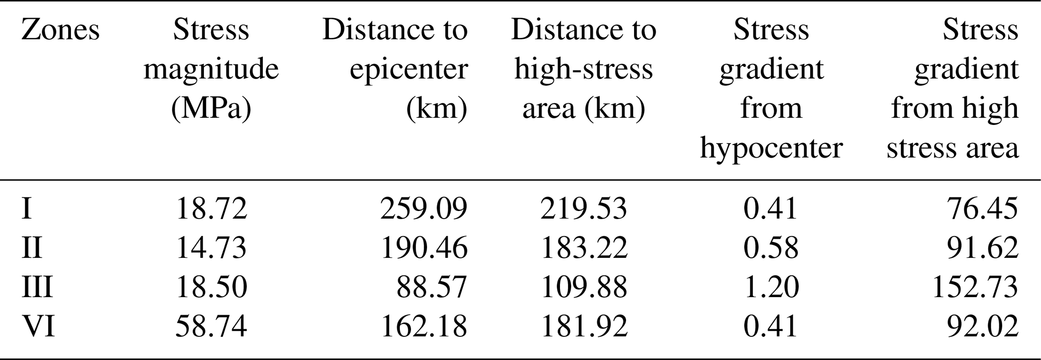
In addition, the high-stress areas are mainly concentrated in the central study area and in the northeast, with lower stress appearing in the southeast and southwest, indicating the existence of a stress gradient toward the southeast and western sides. P-hole generation occurs not only at the hypocenter but also in areas of high-stress concentration. Based on the simulated CSFA, the hypocenter and its nearby high-stress area were selected as the places where the p-holes activations were generated (at a depth of about 15 km). The stress gradients from the hypocenter or the nearby high- stress areas to the four seismic MBT zones were calculated by dividing the stress difference by the distance. The results are shown in Table 4, and the corresponding stress profiles are described in Fig. 7. P-holes could be activated from the hypocenter or from nearby high-stress areas; thus, there was a possibility of p-holes transferring along the stress gradient to all four seismic MBT regions. It is also clear that the closer to the hypocenter or to the high-stress area, the higher the stress gradient.

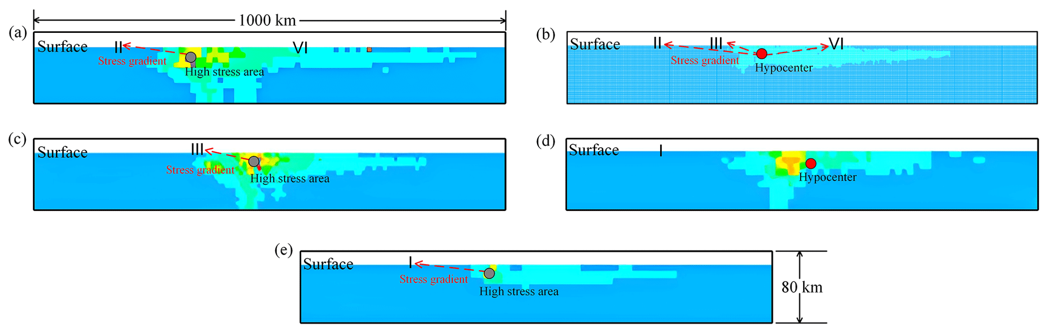
Figure 7 Vertical sections of crustal stress from the hypocenter or nearby high-stress areas to the four seismic MBT zones. Panels (b) and (d) are vertical profiles through the hypocenter, while panels (a), (c), and (e) are the vertical profiles started in the nearby high-stress concentration areas.

Table 4 Stress gradients from the two p-hole activation areas to the four residual MBT regions in Fig. 4.

In summary, the positive MBT anomalies that appeared in zones I, II, III, and VI during the 14 d before the EQ were identified to be possibly related to seismic activity. Positive MBT anomalies in the ground surface due to CSFA indicate the occurrence of p-hole aggregation, which provides the conditions for air ionization in the near-surface atmosphere.

4.2 Scrutiny of seismic AEF anomalies

After screening for negative AEF anomalies, noticeable differences in both space and time between the sites and the regions with positive MBT anomalies were found. Therefore, positive ions generated by p-hole-ionized air can spread in the atmosphere and drift to the sites within the wind field. By analyzing the near-surface wind direction and wind speed, it can be determined if a wind field between the site and the regions with positive MBT anomalies exists. In this study, wind field data at 10 m above the ground with a temporal resolution of 1 h were used. Considering that the wind speed in the entire study area was below 8 m s⁻¹, the distance over which atmospheric ions could have been transported by the wind field was greatly limited. This limitation was the result of neutralization caused by electrostatic interactions and the absorption of aerosols (Wright et al., 2020). Therefore, only the wind fields in the zone of positive MBT anomalies nearest to the AEF sites were taken into consideration.

Negative AEF anomalies can be divided into two categories. The first is that the wind field in the MBT anomaly area did not show a trend moving towards the AEF site, such as the negative AEF anomaly at GAR on 22, 23, and 26 August and at LES on 24 August and 2 September. In Fig. 8a, the MBT residual and SSM residual images were both from 02:00 LT on 22 August, and the wind direction and speed were from 01:00, 04:00, 07:00, and 09:00 LT. The wind direction from zone I to GAR was not indicated before and during the MBT anomaly, and the wind speed was too low to transfer the positive ions generated on the ground surface in zone I to GAR; thus, the negative AEF anomaly at GAR on that day did not result from seismic activity. The other 4 d all showed the same situation as this day.

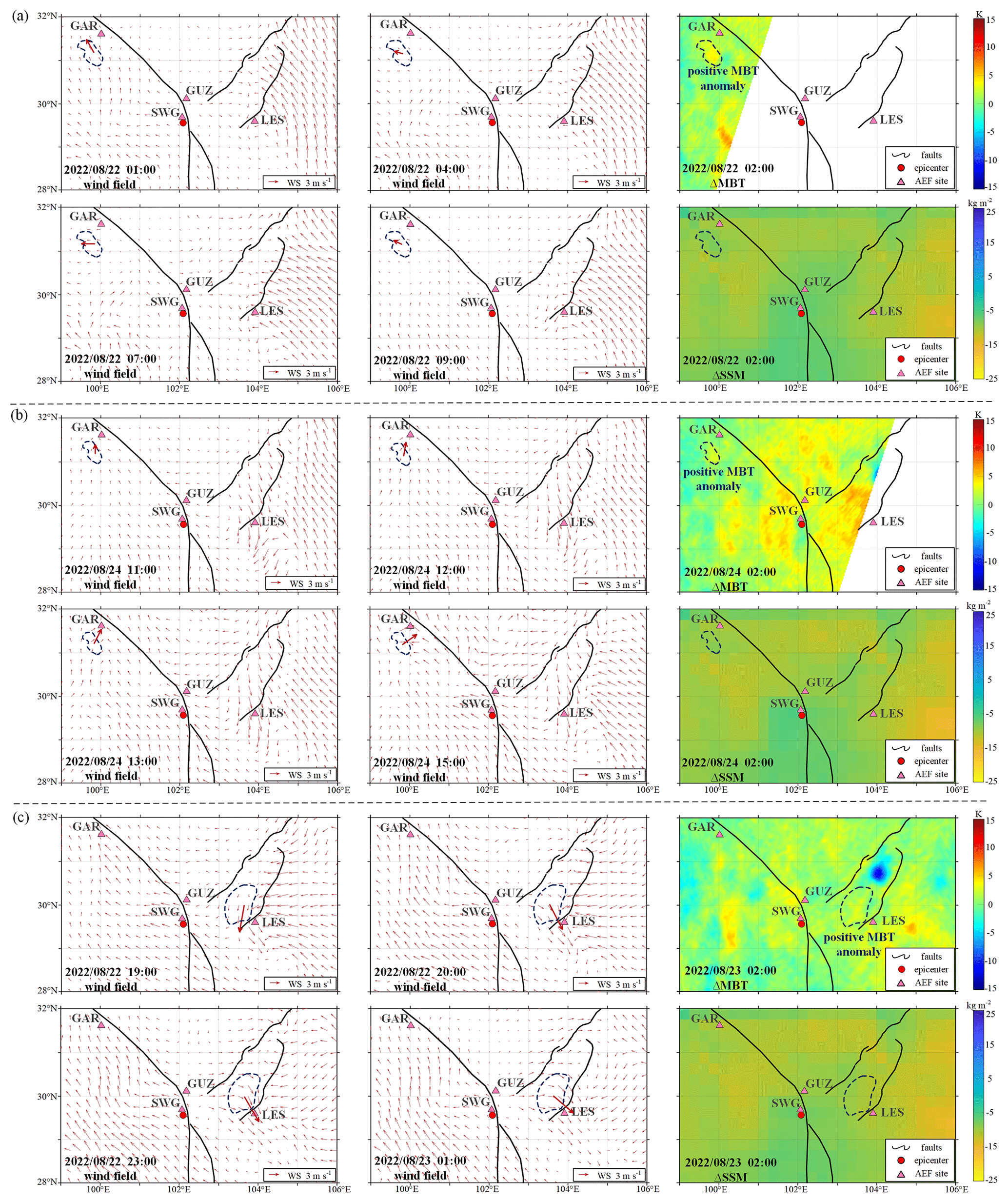
Figure 8 Wind field, MBT residuals, and SSM residuals in the study area on 22 August (a) and 24 August (b) for GAR, and on 22 August for LES (c).

The second category is that the wind field in the area of positive MBT anomalies was pointed towards the AEF sites, such as in the case of the negative AEF anomalies at GAR on 24 August and at LES on 22 August. In Fig. 8b, the AEF anomaly at GAR appeared between 13:00 and 15:00 LT on 24 August. Before 11:00 LT, the wind direction in zone I was slightly to the west of the site. The wind direction began to deflect to the northeast at 12:00 LT, with the direction pointing to the site and maintaining the direction until 14:00 LT, during which time the wind speed gradually increased. The wind deflected to the northeast again at 15:00 LT and then gradually deviated. The wind field changes during this period coincide well with the appearance of the negative AEF anomaly, and the wind field at the site at the end of the anomaly period was also changing. Thus, a longer period of AEF anomaly caused by positive ions staying and accumulating at the site can be ruled out, which is also consistent with the AEF returning to positive levels after 15:00 LT. Therefore, the negative AEF anomaly at GAR on 24 August likely was influenced by seismic activity. In Fig. 8c, the AEF anomaly appeared between 20:00 and 23:00 LT on 22 August at LES. The wind field was pointing west of the AEF site before the anomaly appeared and then veered east and pointed towards the site from 20:00 to 23:00 LT. Then, the wind field continued to veer east and drifted away from the site at 01:00 LT the next morning. The changes in wind field corresponded well to the time of the appearance of the negative AEF anomaly, which shows that seismic activity might have had an impact on the AEF anomaly at that time.

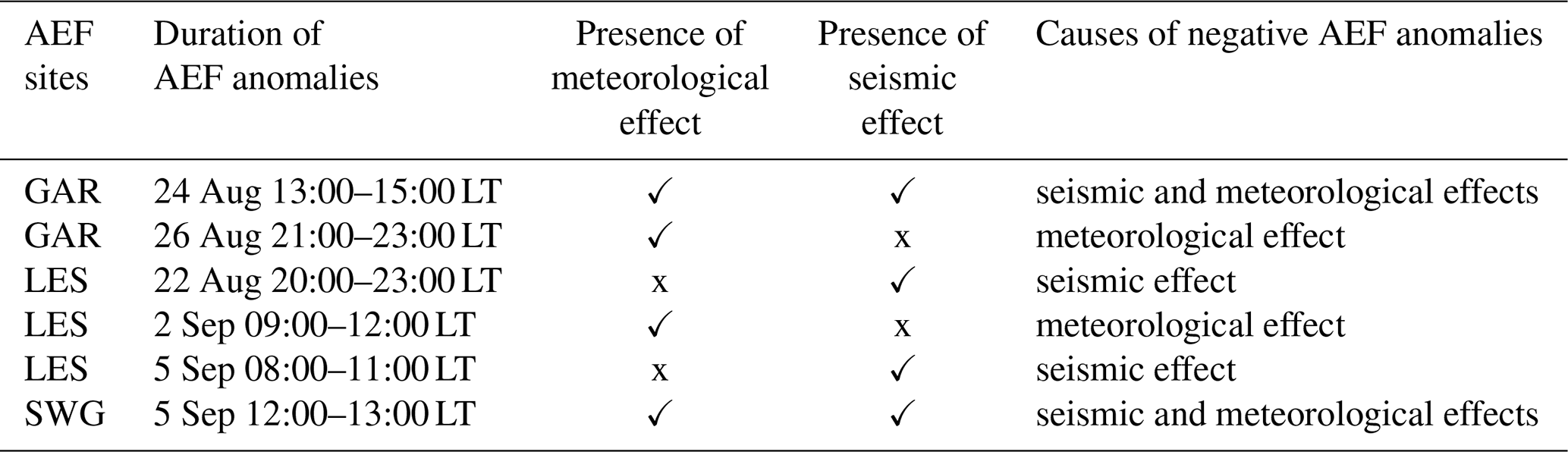
Table 5 Summary of the AEF anomalies before the Luding EQ on 5 September 2022.

On the coseismic day, although there were AEF anomalies at LES and at SWG, the MBT data were missing due to satellite coverage. Taking into account the fact that the surface lithology at both sites was similar to that of the closest MBT anomaly area and that the negative AEF anomaly emerged only 4 h prior to the EQ, it can be inferred that a localized p-hole aggregation phenomenon may have occurred in the immediate vicinity as a direct consequence of seismic activity. This phenomenon would have led to air ionization, thereby altering the vertical AEF.

In conclusion, the negative AEF anomalies observed at GAR from 13:00 to 15:00 LT on 24 August and at LES from 18:00 to 19:00 LT on 22 August are believed to be related to the surface p-hole accumulation caused by seismic activity. The anomalous AEF signals at LES and at SWG 4 h before the EQ on 5 September are considered to be associated with localized changes in atmospheric ion concentrations due to seismic activity during the short imminent stage of the Luding EQ.

5 Conclusions

In this study, historical AEF data from four AEF observatories, namely GAR, LES, GUZ, and SWG, were collected to construct and analyze the FW-AEF. The curves of the FW-AEF exhibited positive fluctuation states and were characterized by single or double peaks. Subsequently, the AEF variations occurring 15 d prior to the Luding EQ in 2022 were meticulously examined, using the FW-AEF as a reference state. As a result, nine AEF negative anomalies (four at GAR, four at LES, and one at SWG) were identified as potentially related to the Luding EQ. This conclusion was reached by analyzing meteorological parameters including CBH, LCC, and TP and space weather parameters including Dst, AE, and SSN. Furthermore, the MBT residuals during the 15 d prior to the Luding EQ were comprehensively analyzed in conjunction with SSM, geological maps, and numerically simulated CSFA. The geophysical environment for high-stress concentration in the Earth's crust and positive charge carrier transfer to and accumulation on the Earth's surface were proven to exist, which meets the conditions for producing seismic AEF anomalies. Furthermore, ground-based wind field data were utilized to investigate the causes of the negative AEF anomalies, taking into account the spatial differentiation between the AEF observatory locations and the areas where positive charge carriers accumulated. The confirmed causes of the AEF anomalies are listed in Table 5.

The negative seismic AEF anomalies that appeared preceding the Luding EQ in 2022 were ascribed to the positive charge carriers generated in areas with high-stress concentration which then accumulated on the ground surface. These charge carriers are capable of ionizing the near-surface air in the surrounding atmosphere, leading to the observed anomalies. This action mechanism serves as a link to establish the coupling process between the coversphere and the atmosphere, which is crucial for an understanding of multiple seismic anomalies. The work identifying and assessing seismic AEF anomalies that was carried out and reported in this study is anticipated to offer a valuable example for future research in this field.