Reconstructing hail days in Switzerland with statistical models (1959–2022)

Hail is one of the costliest natural hazards in Switzerland and causes extensive damage to agriculture, cars, and infrastructure each year. In a warming climate, hail frequency and its patterns of occurrence are expected to change, which is why understanding the long-term variability and its drivers is essential. This study presents new multidecadal daily hail time series for northern and southern Switzerland from 1959 to 2022. Daily radar hail proxies and environmental predictor variables from ERA5 reanalysis are used to build an ensemble statistical model for predicting past hail occurrence. Hail days are identified from operational radar-derived probability of hail (POH) data for two study domains, the north and south of the Swiss Alps. We use data from 2002 to 2022 during the convective season from April to September. A day is defined as a hail day when POH surpasses 80 % for a minimum footprint area of the two domains. Separate logistic regression and logistic generalized additive models (GAMs) are built for each domain and combined in an ensemble prediction to reconstruct the final time series. Overall, the models are able to describe the observed time series well. Historical hail reports are used for comparing years with the most and least hail days. For the northern and southern domains, the time series both show a significant positive trend in yearly aggregated hail days from 1959 to 2022. The trend is still positive and significant when considering only the period of 1979–2022. In all models, the trends are driven by moisture and instability predictors. The last 2 decades show a considerable increase in hail days, which is the strongest in May and June. The seasonal cycle has not shifted systematically across decades. This time series allows us to study the local and remote drivers of the interannual variability and seasonality of Swiss hail occurrence.

1 Introduction

During the convective season, hail causes substantial damage to agriculture, cars, and buildings in Switzerland (BAFU, 2012). One extreme hailstorm on 21 June 2021 caused building damage of CHF 400 million (approx. EUR 415 million) in a single canton alone (Schmid et al., 2024; Kopp et al., 2023). Addressing hail hazard is challenging, as hail is associated with complex interactions of thunderstorm dynamics with microphysical processes that are modulated by synoptic-scale dynamics. Predicting the development and evolution of convective storms is especially challenging in the complex topography of western Europe. Orography such as the Alps and Jura Mountains can initiate or modulate convection, for example by increasing environmental wind shear, which can lead to stronger storm organization (Kaltenböck and Steinheimer, 2015; Kunz et al., 2018). In a changing climate, we may also expect changes in hail frequency and intensity. Although some studies report indications of increasing hail frequency and size (Púčik et al., 2019; Raupach et al., 2023a; Battaglioli et al., 2023a) and hail damage (Willemse, 1995) in Europe, other studies show a negative trend or no trend (Manzato et al., 2022; Augenstein et al., 2023). Trends in damage are not necessarily driven by trends in the hazard. Damage is also linked to exposure and vulnerability and undergoes changes with urban expansion and changes in the built infrastructure.

The pre-Alpine regions north and south of the Alps are regularly affected by severe hailstorms (Nisi et al., 2016; Fluck et al., 2021). Swiss hail occurrence exhibits a strong year-to-year variability and follows a pronounced seasonal cycle (Schröer et al., 2023). Recent studies (Nisi et al., 2018, 2020; Barras et al., 2021; Schröer et al., 2023) have highlighted substantial differences in both interannual and intra-annual hail variability between the northern and southern sides of the Alps. In the northern domain the peak of the convective season typically occurs in June, whereas in the south, it occurs in July (Fig. 2). Moreover, the occurrence of hail-prone and hail-sparse years differs between the two regions.

In contrast to North America, where important drivers of the year-to-year variability of severe convection and hail have been well studied (Tippett et al., 2015; Allen et al., 2020; Taszarek et al., 2020a; Nixon et al., 2023), a thorough examination of the long-term variability of hail in Switzerland is currently lacking. The lack of long-term direct hail observations often hinders the analysis of hail frequency patterns and variability (Martius et al., 2015). To be able to analyze long-term trends and variability in hail occurrence, we need a hail time series longer than anything currently available. Environmental hail proxies derived from sounding, reanalysis, or model data combined with statistical models are typically used to create such extended time series. The primary advantage of reanalysis data is their spatial and temporal coverage and their availability over long time periods. Here, we use ERA5 data to produce a multidecadal daily hail time series for northern and southern Switzerland from 1959 to 2022. ERA5 is considered one of the most reliable reanalyses in representing convective storm environments (Li et al., 2020; Taszarek et al., 2020b; Pilguj et al., 2022; Varga and Breuer, 2022; Wu et al., 2024).

The development of deep moist convection requires an unstable atmosphere, sufficient moisture at low levels, sufficient vertical wind shear, and an initiation mechanism (Johns and Doswell, 1992; Doswell et al., 1996). For hailstones to form in a storm, three additional elements are needed: an embryo particle (typically graupel or frozen drops), an abundance of supercooled liquid water, and sufficient time for the hailstone to grow within the storm's updraft (Allen et al., 2020; Kumjian and Lombardo, 2020; Kumjian et al., 2021). Regional characteristics such as terrain barriers, local wind systems, and warm water surfaces influence the relative importance of these elements necessary for hailstorm development, which is why this study looks at the regions north and south of the Alps separately.

Convection in the region south of the Alps is influenced by the transport of moist and warm air masses originating from the Adriatic and Mediterranean seas during southwesterly or southern flow conditions (e.g., Nisi et al., 2016). These air masses create ideal conditions for convective storm development, when coupled with local wind systems such as mountain–plain circulations and valley breezes. Previous studies have highlighted the relevance of anabatic–katabatic wind systems to hail formation in the southern pre-Alpine region and specifically in the Po Valley (Morgan, 1973; Gladich et al., 2011). The southern domain is shielded from northern air masses by the Alpine chain, whereas the northern domain is regularly exposed to frontal systems originating from the west or north (Schemm et al., 2016).

Due to these unique topographic and synoptic conditions, predicting hailstorm formation in Switzerland requires regional-specific models that consider individual interactions. Various atmospheric variables have been used in statistical models to predict severe hail-producing thunderstorms in Europe (Groenemeijer and van Delden, 2007; Kunz, 2007; García-Ortega et al., 2012; Manzato, 2012; Mohr and Kunz, 2013; Gascón et al., 2015; Púčik et al., 2015; Tuovinen et al., 2015; Melcón et al., 2017). There are regional differences from the United States (Brooks et al., 2003; Rasmussen, 2003; Johnson and Sugden, 2021; Taszarek et al., 2020a; Nixon et al., 2023) and Australia (Allen et al., 2011; Raupach et al., 2023a). Mohr and Kunz (2013) and Kunz (2007) presented a comprehensive list of hail-relevant meteorological parameters and indices that can be used as environmental proxies for Europe, and Huntrieser et al. (1997) presented a list specifically for Switzerland.

The parameters and indices can be grouped into three categories: instability and moisture, which are both thermodynamic, and kinematic conditions. Latent, conditional, and potential instabilities are captured by indices such as convective available potential energy (CAPE) (Moncrieff and Miller, 1976), the lifted index (Galway, 1956), the vertical totals index (Miller, 1972), the Boyden index (Boyden, 1963), the Showalter index (Showalter, 1953), and the KO index (Andersson et al., 1989). Other indices combine all three instabilities, such as the total totals (Miller, 1972) and K indices (George, 1961). Other indices measure the tropospheric moisture content, such as vertically integrated liquid water (Greene and Clark, 1972), and kinematic conditions, such as the magnitude of the vertical wind shear (Weisman and Klemp, 1982, 1984). Composite parameters that combine kinematic and thermodynamic variables such as the SWISS index (Huntrieser et al., 1997), the significant hail parameter (SHIP), and the hail size index (HSI) also correlate well with the occurrence of large hail (Allen et al., 2015; Czernecki et al., 2019; Gensini et al., 2021; Johnson and Sugden, 2021). The indices are then used in statistical models to estimate the occurrence of hail.

For instance, Mohr et al. (2015a) used a logistic regression approach to estimate the potential for hailstorms in Germany between 1971 and 2000 and between 2021 and 2050. They find that the potential for hail events is projected to increase significantly in 2021–2050 compared to 1971–2000 in the northwest and south of Germany.

Logistic regression has also been used by Billet et al. (1997), Schmeits et al. (2005), Sánchez et al. (2009), and López et al. (2007) to model thunderstorm and hail events. Recently, Battaglioli et al. (2023a) created a logistic generalized additive model for Europe and the United States from European Severe Weather Database (ESWD) reports and ERA5 data to model trends of large hail (>2 and >5 cm) occurrence. They presented a significant increase in hail frequency in northern Italy and parts of southern Switzerland. Allen et al. (2015) developed a Poisson regression from monthly averages to connect monthly hail frequency to the large-scale atmospheric environment in the United States. Madonna et al. (2018) presented a Poisson regression hail model using radar and ERA5 data specifically for northern Switzerland. Their model captured the intra-annual and interannual hail variability well, and their time series showed an increase of 0.5 hail days per month per decade.

We build on the work of Madonna et al. (2018), but in this study, we increase the resolution of the analysis to daily, we additionally include the south of Switzerland, and we extend the time series back to 1959. Unlike Battaglioli et al. (2023a), who used ESWD severe-weather reports, we use Swiss radar data as proxies to model hail day occurrence. Furthermore, we employ an ensemble of two statistical models, a logistic multiple regression and a logistic generalized additive model (GAM), to leverage the best-fitting predictors for each domain individually. Our statistical models are tailored to Switzerland. Our goal is not to build a model for forecasting, but we want to produce the best possible reconstruction of past hail days in Switzerland from environmental predictor variables. The statistically modeled time series will then be used to study long-term trends and changes in the frequency, seasonality, and variability of model-derived Swiss hailstorms in past decades.

The paper is structured as follows. Section 2 provides an overview of the datasets used in this study and is followed by a description of methods in Sect. 3. Model building and performance are explained in Sect. 4. Results from time series analyses are presented in Sect. 5, which are discussed in Sect. 6. Conclusions follow in Sect. 7.

2 Data

2.1 Radar-derived probability of hail

This study uses the radar- and model-based probability of hail (POH) product as a proxy for hail. POH is an empirical hail detection algorithm from MeteoSwiss that indicates the probability of hail of any size on the ground from 0 % to 100 %. The estimate follows the method of Foote et al. (2005) and Waldvogel et al. (1979) and is based on the vertical distance between the 45 dBZ echo top height measured by the Swiss radar network and the freezing level height obtained from the COSMO-CH numerical weather forecast model (Baldauf et al., 2011); see Nisi et al. (2016) and Kopp et al. (2024) for a detailed description of the POH algorithm. POH is currently available from 2002 to 2024 in 5 min and daily time intervals on a 1 km × 1 km Cartesian grid spacing. The third-generation Swiss radar network, which from 2002 to 2012 consisted of three single-polarization Doppler C-band radars, was updated to the more advanced fourth-generation dual-polarization Doppler C-band radars in 2012. Subsequently, two additional radars were installed in mountainous regions at high elevations, where orographic beam blocking minimized low-level interference from the other three radars. We use thoroughly quality-checked and reprocessed POH data from the recently published Swiss hail climatology (Trefalt et al., 2023; Schröer et al., 2023) and consider areas within a 140 km radius around the five radar stations (Fig. 1). The 140 km radius limitation helps minimize planar artifacts and ground clutter.

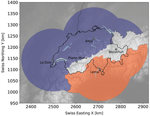
Figure 1 The dots indicate the locations of the five radars (La Dôle, Albis, Monte Lema, Plaine Mort, and Weissfluh). The shading indicates the two study areas north of the Alps (blue) and south of the Alps (orange). The areas are within a 140 km radius of the five MeteoSwiss weather radars (black circles) overlaid on a digital elevation map (gray shading, source: Federal Office of Topography swisstopo).

The central Alps are excluded from the analysis because hail rarely occurs there (Van Delden, 2001; Giaiotti et al., 2003; Nisi et al., 2016) and radar quality may be lower (Feldmann et al., 2021). The central Alps are delineated from the northern and southern pre-Alps by the boundaries of the official prognosis regions from the Federal Office of Meteorology and Climatology MeteoSwiss. This selection of the study domains allows the climatological regimes north and south of the Alps to be separated and corresponds to those in Barras et al. (2021). Comparing POH data with car insurance loss data, Nisi et al. (2016) showed that a POH threshold of 80 % best represents hail locally. Note that damage occurs to cars with hailstone sizes of around 2 cm and larger. More information on the definition of hail days is provided in Sect. 3.1.

2.1.1 ERA5 environmental predictors

For multidecadal analyses, ERA5 is the best product currently available for Europe. Therefore, we use ERA5 reanalysis data to quantify the hail potential of the atmosphere (Hersbach et al., 2020). In this work, data from 1959 to 2022 at hourly and 6-hourly intervals were used, including model levels (137 levels from 1000 to 1 hPa, 0.5°×0.5° grid spacing), pressure levels (17 levels, 0.5°×0.5° grid spacing), and surface data (0.25°×0.25° grid spacing). We exclude any data before 1959 from our analysis because the quality of ERA5 declines in those years (Bell et al., 2021) and cannot be used to analyze trends. A total of 75 convective parameters was calculated (Table S1 in the Supplement).

Statistical models classifying hail events typically select the ERA5 grid point that is temporally and spatially closest to the hail incident. However, such a selection is not possible for reconstructing past hail events because no information is available on the hail event prior to the observational period. Therefore, to model the occurrence of a hail day, we calculate ERA5 profiles averaged across the entire northern or southern domains at 12:00 UTC. The values at 12:00 UTC exhibited the highest predictive skill, which may be attributed to the fact that most storms in Switzerland occur in the late afternoon (e.g., Nisi et al., 2016, 2018). Thus, the 12:00 UTC value is most likely to capture the atmospheric conditions before storm formation.

Our definition of hail days focuses on days with more than a single hail cell. The thresholds are set to capture events that led to damage and affected somewhat larger areas (probability of hail ≥ 80 % over a minimum area of 580 km² for the northern domain and 499 km² for the southern domain, as detailed in Sect. 3.1).

2.2 Historic hail data

To check plausibility, we compared the modeled time series to a historical hail dataset that is a qualitative combination of multiple data sources, mainly crop damage reports, extending back to 1825, and early radar data, including research radar data extending back to 1983 (Müller and Schmutz, 2021). Most relevant for our study period, 1959–2022, is the agricultural crop damage data archive by the Swiss agricultural hail insurance company Schweizer Hagel. Radar-based measurements complement the archive after 2002. The historical information is temporally resolved on a daily scale and spatially resolved on a municipality scale. From this information, we derived a time series with binary hail information using a threshold of five affected municipalities. The threshold was selected to best match the annually averaged hail days derived from POH data (see Sect. 3.1). This historical data archive is subject to significant uncertainties, including reporting biases, changing vulnerabilities and exposures of crop cultures, hail prevention measures, the fraction of insurance partition, and mergers of municipalities (Willemse, 1995). Due to these limitations, the historical data cannot be interpreted as a homogeneous time series, and a quantitative comparison is impossible. However, the data contain valuable information on the weakest and strongest active hail years and an indication of multiyear variability, which can complement model evaluation.

3 Methods

In this section, we first provide an explanation of how hail days are extracted using the probability of hail (POH) radar proxies and then analyze the distribution of the POH time series.

3.1 POH time series

To identify hail days in northern and southern Switzerland, we use daily POH data from 2002 to 2022 during the hail-prone months of April to September. We use the same domains and area thresholds as Barras et al. (2021). The daily area of POH ≥ 80 % is extracted separately for the domains north and south of the Alps (Fig. 1). To qualify as a hail day, the daily maximum POH must reach or exceed 80 % over an area of at least 580 km² in the northern domain and 499 km² in the southern domain. Barras et al. (2021) determined that these thresholds correlate best with days when car damage was reported across Switzerland from 2002 to 2012. This definition implies hail large enough to cause damage to cars, approximately 2 cm in size. The sensitivity of our models to this threshold was tested by varying the area threshold. We found no significant impact on misses or false alarms, consistent with earlier studies indicating low sensitivity to area thresholds (Madonna et al., 2018). These criteria yield 566 hail days in the northern domain and 560 in the southern domain between 2002 and 2022. The a priori probability of hail days between 1 April and 30 September is 14.7 % in the north and 14.5 % in the south.

On average, 27.0 hail days per year occurs in the north and 26.7 in the south. A maximum of 44 hail days was recorded in the north in 2009 and a maximum of 37 in the south in 2018. A minimum of 16 hail days occurred in the northern domain in 2020 and a minimum of 17 hail days in the southern domain in 2007.

There is considerable interannual variability with domain-specific differences during the observation period (Fig. 2a). While the most recent years in the south show a frequency above the average, the opposite is true in the north. Yet, with a time series of only 20 years, we cannot assess or interpret trends in a robust way.

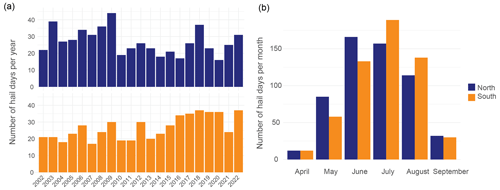
Figure 2 The number of yearly (a) and monthly (b) hail days for the northern (blue) and southern (orange) domains for 2002–2022.

Hail is a seasonal phenomenon with a strong annual cycle in both domains (Fig. 2b). In the north, hail is most frequent in June, with a total of 166 hail days, followed by July with 157 hail days. In the south, hail is most frequent in July with 189 hail days.

4 Statistical model development and model performance

This section offers an overview of the development of the four statistical models and an evaluation of their performance. We discuss the development and performance of the individual logistic regression models (Sect. 4.1), the generalized additive models (GAMs) (Sect. 4.2), and the ensemble prediction (Sect. 4.3).

4.1 Logistic regression

Applequist et al. (2002) suggest multiple logistic regression as an appropriate tool for a binary classification problem, and logistic regression models have been used effectively in many studies to model the occurrence of hail- and thunderstorms (e.g., Billet et al., 1997; Schmeits et al., 2005; Sánchez et al., 2009; Battaglioli et al., 2023a). A multiple logistic regression model predicts the occurrence probability p of hail as a function of several environmental parameters (x₁, x₂, …, x_n) as independent variables (Hosmer and Lemeshow, 2000). A binary variable, here hail yes/no, is defined as a dependent variable y. The occurrence probability p(x) is defined as

$$\begin{array}{}\text{(1)}& y=p\left(x\right)=\mathrm{1}/\left(\mathrm{1}+e^{-g\left(x\right)}\right),\mathrm{where}\mathrm{0}\le p\left(x\right)\le \mathrm{1}.\end{array}$$

The model is based on a linear regression:

$$\begin{array}{}\text{(2)}& g\left(x\right)={\mathit{\beta }}_{\mathrm{0}}+{\mathit{\beta }}_{\mathrm{1}}\times x_{\mathrm{1}}+{\mathit{\beta }}_{\mathrm{2}}\times x_{\mathrm{2}}+\mathrm{\dots }+{\mathit{\beta }}_n\times x_n.\end{array}$$

We computed the regression coefficients β_n in R with the glm package using the maximum-likelihood method. The dataset was divided into training and test sets by distributing data points from 2012 to 2022 randomly into 70 % and 30 %. Additionally, we used the POH data from 2002 to 2011 as an independent validation set to prevent overfitting. To estimate the performance of the model, we used 10-fold cross-validation. A total of 75 different convective and meteorological parameters were tested as predictors x_n (Table S1). The best models were chosen by comparing multiple performance metrics. We considered the Akaike information criterion (AIC), the Bayesian information criterion (BIC), the critical success index (CSI) or threat score, the probability of detection (POD), the false alarm ratio (FAR), the success ratio (SR), and the Heidke skill score (HSS), as well as the bias, precision, and accuracy values. The metrics were calculated from contingency tables by averaging over the 10 test, training, and validation data subsets. Equations for the contingency table metrics, AIC, and BIC can be found in Table A1.

We use a combination of multiple metrics to build a model with the optimal balance between over- and underfitting. The correct prediction of hits is of slightly greater importance than false alarms because finding hail days is our main priority. We also avoided multicollinearity between predictor variables by requiring the variance inflation factor (VIF; Mansfield and Helms, 1982) of any predictor to remain below 4. We use a probability threshold of p(hail)≥0.4 for the north and p(hail)≥0.44 for the south to identify hail days. This threshold was identified by examining ROC curves and plots of modeled vs. observed hail days.

A residual analysis was performed to ensure no systematic errors remained in the model residuals. We looked at the yearly and monthly averaged residuals of the 10 training and test data subsets separately. A strong increase in the variance of yearly residuals was present in data points before 2012, which warranted our decision to only use POH data from 2012 onwards for training. In 2012, the Swiss radar network underwent a major update. Even though we reduced the size of the training dataset, the predictive skill of the models for both domains increased slightly. Furthermore, we introduce a categorical variable, month, as an additive factor in both models, containing the 6 months of April through September. This addition was intended to reduce the nonstationarities associated with a seasonal cycle. Residuals were more regular after the inclusion of the month factor, and the model's predictive skill increased.

To find the optimal number of predictors, we applied a manual stepwise forward method, resulting in five predictors and the month factor for both the northern and the southern models. The best logistic models for each are

$$\begin{array}{}\text{(3)}& \begin{array}{rl}g\left(\mathrm{hail}\right)& ={\mathit{\beta }}_{\mathrm{0}}+{\mathit{\beta }}_{\mathrm{1}}\times \mathrm{LI}+{\mathit{\beta }}_{\mathrm{2}}\times \mathrm{TT}+{\mathit{\beta }}_{\mathrm{3}}\times \mathrm{omega}\mathrm{\_}\mathrm{vint}\\ & +{\mathit{\beta }}_{\mathrm{4}}\times \mathrm{q}\mathrm{\_}\mathrm{vint}+{\mathit{\beta }}_{\mathrm{5}}\times \mathrm{BI}+\sum _{n=\mathrm{5}}^{\mathrm{9}}{\mathit{\beta }}_n\times {\mathrm{1}}_{\mathrm{month}=n+\mathrm{1}}\end{array}\end{array}$$

for the northern model and

$$\begin{array}{}\text{(4)}& \begin{array}{rl}g\left(\mathrm{hail}\right)& ={\mathit{\beta }}_{\mathrm{0}}+{\mathit{\beta }}_{\mathrm{1}}\times \mathrm{LI}+{\mathit{\beta }}_{\mathrm{2}}\times \mathrm{KI}+{\mathit{\beta }}_{\mathrm{3}}\times \mathrm{v}\mathrm{\_}\mathrm{500}+{\mathit{\beta }}_{\mathrm{4}}\\ & \times \mathrm{SP}+{\mathit{\beta }}_{\mathrm{5}}\times \mathrm{TT}+\sum _{n=\mathrm{5}}^{\mathrm{9}}{\mathit{\beta }}_n\times {\mathrm{1}}_{\mathrm{month}=n+\mathrm{1}}\end{array}\end{array}$$

for the southern model.

LI is the surface-based lifted index. TT is the total totals index, omega_vint is the vertically integrated vertical velocity, q_vint is the vertically integrated specific humidity, BI is the Boyden index, KI is the K index, v_500 is the meridional component of the wind at 500 hPa, and SP is the mean surface pressure. Descriptions, mean values, and percentiles of all variables can be found in Tables S1 to S3. A detailed evaluation of the performance of the final ensemble prediction is undertaken in Sect. 4.3. Here, we discuss the performance metrics of the logistic models summarized in Table 1.

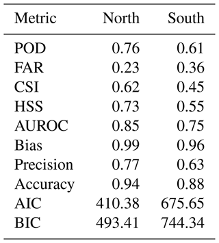
Table 1 Performance metrics of the logistic model for north and south. Metrics are calculated from k-fold cross-validation and are the averages of the test datasets. For POD, CSI, HSS, AUROC, bias, precision, and accuracy, a value close to 1 indicates good performance, whereas FAR, AIC, and BIC should remain as low as possible.

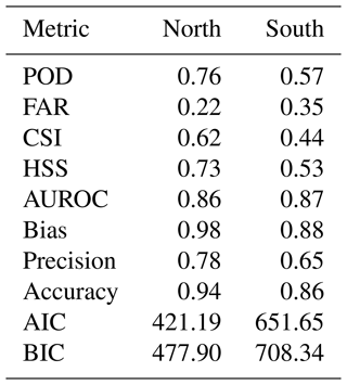
The northern model has a higher POD, lower FAR, and lower CSI than the southern model. The performance metrics suggest that the northern model can distinguish better between hail and no-hail days and misses fewer hail days than the southern model. Nonetheless, when comparing our models to other studies, we rank either better with a lower FAR, as in all studies mentioned in Raupach et al. (2023a), or similar to other studies, as in López et al. (2007) and Gascón et al. (2015).

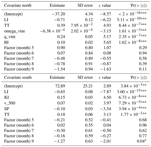
All coefficients and p values of covariates are listed in Table B1. All model predictors except the categorical month factor are significant. Although the month factor was not significant, the model's performance decreased when removing the factor. Possible explanations for the months not being significant in our model include that our sample size is too small for the effect to become significant and that there is multicollinearity between months in the model. Only LI and TT are selected in both models, albeit with different coefficients. The z values in Table B1 show that instability and moisture predictors (LI, KI, q_vint) have the highest feature importance in both models. The z value measures how many standard deviations the coefficients are from 0; hence, the higher the absolute value, the higher the importance.

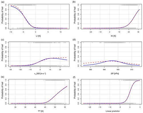
To illustrate the modeled relationship between response and predictors, Figs. 3 and 4 show marginal response plots of the logistic models. In both figures, the response is plotted against each independent model covariate x_n and against the linear combination of all covariates (bottom-right graph) with LOESS smooth functions. The model, represented by the dashed red line, matches the marginal relationships of the data represented by the solid blue lines, and hence all predictors are well fitted and do not need further modification. The gray points show the distribution of the covariates. Some variables have a stronger influence on the model's predicted probability than others. An LI of −5 K translates to a probability of hail of 60 % (Fig. 3a), whereas the highest probability of any omega_vint value reaches less than 30 % (Fig. 3c). In all models, two to three covariates mainly determine the hail occurrence probability, and the remaining covariates are used for fine-tuning.

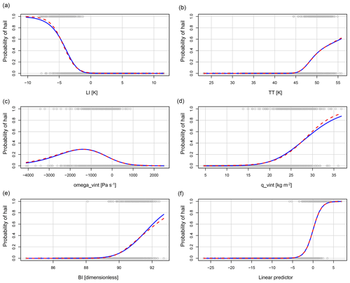
Figure 3 Marginal model plots showing the modeled relationship of each covariate (x axes) to the modeled probability of a hail day (y axes) given all other covariates are held constant at their mean value. The bottom-right graph shows the linear combination of all covariates in their mean function. The model is represented by the dashed red lines, and the marginal relationships of the data are represented by the solid blue lines. The gray points show the distribution of covariates. Some variables have a stronger influence on the model's predicted probability than others.

Figure 4 As Fig. 3 but for the southern domain.

We next briefly discuss how each selected model predictor is connected to environments favoring hail. The surface-based lifted index (LI) is a measure of stability of the atmosphere and is defined as the difference between the temperature at 500 hPa and the temperature of a parcel that is lifted from the surface to its lifted condensation level (LCL) dry adiabatically and then pseudo-adiabatically to 500 hPa. A negative LI indicates atmospheric instability, which is favorable for the development of convective storms. The lower the LI, the more unstable the atmosphere (hailstorms possible at an LI of approx. −4 K; Kunz, 2007). This relationship matches the models' fitted negative linear relationship in both domains (Figs. 3a and 4a).

The total totals (TT) index combines two components, the vertical totals (VT) and the cross totals (CT). The VT reflects static stability or the lapse rate between 850 and 500 hPa. The CT includes the 850 hPa dew point temperature. As a result, TT increases with decreasing static stability and increasing 850 hPa moisture, but it does not capture the moisture below the 850 hPa level. Additionally, convection may be inhibited despite a high TT value if a significant capping inversion is present. A TT of 50 K or larger usually indicates that hailstorms are possible (Mohr and Kunz, 2013). In the northern and southern models, the probability of hail exceeds 50 %, with TT values of approximately 52 K (Figs. 3b and 4e).

The K index (KI), like the VT, is based on the vertical temperature gradient between 850 and 500 hPa and dew point temperatures at 850 and 700 hPa. Higher humidity at 850 hPa, expressed by higher dew point temperatures at 850 hPa, increases the KI. Furthermore, lower humidity at higher levels (700 hPa) decreases the chance of thunder- or hailstorms occurring. The higher the KI, the higher is the probability of a hailstorm. KI above 20–30 K usually indicates possible thunder- or hailstorms (Kunz, 2007), which matches our relationship of KI to hail in the southern model (Fig. 4b).

The Boyden index (BI) was originally developed to assess the thunderstorm risk in frontal passages. This convective parameter does not include information on humidity. It considers the temperature at 700 hPa and the thickness of the 1000–700 hPa layer, which is proportional to its temperature. The higher the value of the BI, the greater is the risk of thunderstorms. The threshold value for thunderstorms is approximately 95 (Boyden, 1963), which is slightly higher than what the model learns for the northern domain (50 % probability of hail at a BI greater than approx. 90, Fig. 3e). As mentioned in Sect. 1, on the north side of the Alps, around 20 %–40 % of Swiss hailstorms are associated with fronts, which is probably why that parameter was chosen and why it is highly important in the model.

The vertically integrated vertical velocity (omega_vint) denotes the vertical motion of air throughout the atmospheric column and primarily reflects large-scale synoptic ascent or descent. In our model, the highest probabilities of hail occur when omega_vint values are negative (Fig. 3c), signifying large-scale ascent.

The vertically integrated specific humidity (q_vint) quantifies the total amount of water vapor available in the atmospheric column and thus indicates the moisture available for hailstorm development. Consequently, a higher q_vint increases hail day probability (Fig. 3d).

Finally, v_500, the meridional component of the wind at 500 hPa, and the mean surface pressure (SP) might be connected to hailstorm development indirectly. Our model shows that the highest probabilities of hail are achieved with neither very high nor very low pressure (Fig. 4d). A positive sign of v_500 indicates air moving northwards at 500 hPa, which the model translates to higher probabilities of hail in the southern domain (Fig. 4c). This indication could be related to a synoptic situation in the south of Switzerland, where moist, warm air is transported from the Mediterranean towards the Alps (Schemm et al., 2016). The lack of a kinematic predictor in the northern model is discussed further in Sect. 6.1.

All these connections are part of a complex interplay of atmospheric conditions that contribute to hailstorm development. Therefore, we examine combinations of various parameters to assess the likelihood of hailstorms in our models. When the variable combinations from the northern model are applied to the southern domain and vice versa, the coefficients change and the predictive skill declines. This difference in coefficients and predictive skill underlines the necessity of using unique sets of predictors for each domain instead of a single model across all of Switzerland.

Automatic predictor selection procedures such as recursive feature importance and LASSO gave worse-performing models than a manual stepwise approach combined with expert knowledge that was based on earlier considerations of optimal distribution separations of hail vs. no-hail days (Trefalt, 2017) and computed correlations (Figs. S1 and S2 in the Supplement). Further discussions on variable selection and their importance follow in Sect. 6.

4.2 Generalized additive models (GAMs)

As mentioned before, the use of a generalized additive model (GAM) was warranted to account for potential nonlinear and nonparametric correlations in the data that may not be adequately captured by a conventional logistic regression. A GAM is a generalized linear model in which the response variable depends linearly on the smooth functions of the model's predictor variables (Hastie and Tibshirani, 1987). The logistic equation from before (Eq. 2) becomes

$$\begin{array}{}\text{(5)}& g\left(x\right)={\mathit{\beta }}_{\mathrm{0}}+f_{\mathrm{1}}\left(x_{\mathrm{1}}\right)+f_{\mathrm{2}}\left(x_{\mathrm{2}}\right)+\mathrm{\dots }+f_n\left(x_n\right).\end{array}$$

The nonparametric form of the functions f_n enhances the flexibility of the model, but it also imposes constraints on additivity, allowing us to interpret the model in a similar manner as the multiple logistic regression. CAPE appeared more often as a model predictor in the GAMs than in the logistic regression models during model training. Nevertheless, the best model for the northern domain preferred the LI over CAPE. The selection of predictors followed the same procedure as in the logistic regression model. For every variable that presented an effective degree of freedom (edf) > 1, a smoothing spline function was applied to allow for nonlinear effects. The model was fitted with the mgcv R package.

The best GAM in the northern domain is

$$\begin{array}{}\text{(6)}& \begin{array}{rl}g\left(x\right)& ={\mathit{\beta }}_{\mathrm{0}}+f_{\mathrm{1}}\left(\mathrm{LI}\right)+f_{\mathrm{2}}\left(\mathrm{KI}\right)+f_{\mathrm{3}}\left(\mathrm{TT}\right)+f_{\mathrm{4}}\left(\mathbf{z}\mathbf{\_}\mathbf{0}\mathit{°}\mathrm{C}\right)\\ & +f_{\mathrm{5}}\left(\mathrm{WS}\mathrm{\_}\mathrm{06}\right)+f_{\mathrm{6}}\left(\mathrm{WS}\mathrm{\_}\mathrm{36}\right)+\sum _{n=\mathrm{5}}^{\mathrm{9}}{\mathit{\beta }}_n\times {\mathrm{1}}_{\mathrm{month}=n+\mathrm{1}}\end{array}\end{array}$$

and for the southern domain

$$\begin{array}{}\text{(7)}& \begin{array}{rl}g\left(x\right)& ={\mathit{\beta }}_{\mathrm{0}}+f_{\mathrm{1}}\left(\mathrm{CAPE}\right)+f_{\mathrm{2}}\left(\mathrm{WS}\mathrm{\_}\mathrm{06}\right)+f_{\mathrm{3}}\left(\mathrm{Td}\mathrm{\_}\mathrm{2}\mathrm{m}\right)\\ & +f_{\mathrm{4}}\left(\mathrm{TT}\right)+f_{\mathrm{5}}\left(\mathrm{omega}\mathrm{\_}\mathrm{500}\right)+\sum _{n=\mathrm{5}}^{\mathrm{9}}{\mathit{\beta }}_n\times {\mathrm{1}}_{\mathrm{month}=n+\mathrm{1}}.\end{array}\end{array}$$

Here LI is the surface-based lifted index, KI is the K index, TT is the total totals index, z_0 °C is the freezing level, CAPE is the most unstable convective available potential energy computed for parcels departing from model levels below the 350 hPa level, WS_06 is the magnitude of bulk wind shear between 10 m and 6 km, WS_36 is the magnitude of bulk wind shear between 3 and 6 km, Td_2m is the 2 m dew point temperature, and omega_500 is the vertical velocity at 500 hPa. The final five variables do not appear in the logistic regression models. The thresholds for identifying a hail day were set to p(hail)≥0.40 for the north and p(hail)≥0.41 for the south.

In the northern model the combination of LI and TT and in the southern model the combination of CAPE and TT lead to a strong increase in the performance of the model. We therefore allowed composite parameters such as TT in favor of a better predictive performance. The performance measures for the GAMs can be found in Table 2. Both GAMs perform very similarly to the logistic regression models. The northern GAM outperforms the southern model. Table B2 provides the coefficients and their corresponding p values for parametric covariates, and Table B3 details the nonparametric terms. Again, all model predictors except the month factor are significant. The models' explained variances are 63.1 % for the north and 45.5 % for the south.

Table 2 Performance metrics of the GAMs for north and south. Metrics are calculated from k-fold cross-validation and are the average of the test datasets. For POD, CSI, HSS, AUROC, bias, precision, and accuracy, a value close to 1 indicates good performance, whereas FAR, AIC, and BIC should remain as low as possible.

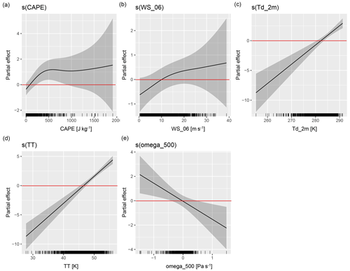
We can visualize the modeled relationship between the response and the covariates once again to reflect how each covariate is connected to hailstorm development. Figures 5 and 6 depict partial dependence plots for both GAMs. Each figure illustrates the partial effect of individual model covariates x_n on the probability of a hail day. The vertical black lines at the bottom represent the distribution of the covariates. The black lines in the gray band are smoothing functions that capture the modeled relationships. The horizontal red lines are the y=0 lines that separate the plot space into a positive and negative partial effect.

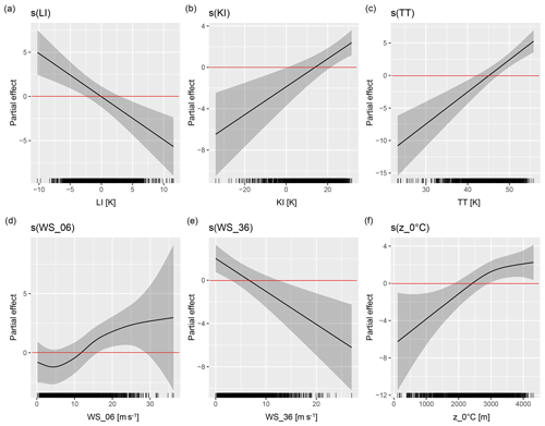
Figure 5 Partial dependence plots for each model covariate in the northern model. The solid black line and gray uncertainty range represent the modeled partial effect of the covariate on the response. The red y=0 lines separate positive from negative effects. The short black vertical lines indicate the covariate distribution.

Figure 6 The same as Fig. 5 but for the southern model.

In the southern model (Fig. 6a–f), the partial effect on the probability of hail is positive when TT≥47 K, Td_2m≥282 K, WS_06≥10 mṡ⁻¹, and CAPE≥100 J kg⁻¹ and when omega_500 is negative.

CAPE is a measure for the energy available for convection. Large positive values of CAPE indicate that an ascending air parcel would be much warmer than its surrounding environment and therefore very buoyant. High CAPE values indicate that high updraft speeds can occur within thunderstorms, allowing the sustained lifting of moist air to colder altitudes where hailstones can form and grow. Our model shows a strong positive effect of CAPE at values of approx. 500 J kg⁻¹. The slope of the curve then flattens towards higher values, which are also where uncertainty increases (Fig. 6a).

WS_06 has a very similar relationship in the southern model, where at least 10 m s⁻¹ is needed for a positive effect, but then the partial effect increases only slightly with increasing magnitude of deep-level shear (Fig. 6b). Shear has the least importance of all predictors in the model.

The dew point temperature at 2 m (Td_2m) quantifies the temperature and moisture at the surface. Higher dew point temperatures imply higher surface temperatures and more moisture in the air. The release of latent heat due to the condensation of moisture enhances buoyancy and thus fosters the development of the strong updrafts necessary for hail formation. Our model shows the highest partial effect for hail occurrence with the highest dew point temperatures (Fig. 6c).

Similar to the vertically integrated vertical velocity omega_vint, the vertical velocity at 500 hPa (omega_500) is a measure for the vertical motion of air, here for the level at 500 hPa. Negative values indicate upward motion. The highest positive effect is achieved with the strongest negative vertical velocities (Fig. 6e).

In the northern model, the partial effect on the predicted probability of the model is positive when LI≤0 K, TT≥45 K, and KI≥15 K (Fig. 5a–f). We explain the relationship of LI, KI, and TT to hailstorm development in Sect. 4.1. The GAMs fit similar linear relationships to the logistic regression models, with higher probabilities of hail achieved with increasing KI and TT and decreasing LI.

Notably, the deep-layer shear WS_06 exhibits a nonlinear relationship to the response variable. WS_06 has its most negative effect at values around 0–10 m s⁻¹, transitioning to a positive effect above 15 m s⁻¹ (Fig. 5d). The curve flattens at very high wind shear values, suggesting that higher shear does not further increase the probability of hail. Additionally, the confidence intervals of smoothing functions widen significantly towards the tails of each covariate distribution.

GAMs are not limited by multicollinearity between model terms, which is why both WS_36 and WS_06 were selected in the northern model. The model preferred including both WS_36 and WS_06 over either one of them, as the individual predictors otherwise became insignificant and less important. Surprisingly, WS_36 has a negative linear relationship with hail in northern Switzerland. To gain a deeper understanding of how the WS_36 and WS_06 model terms interact, we further examined contour plots depicting conditional probabilities based on pairs of model predictors (not shown). The highest probabilities of hail are achieved with high WS_06 but low WS_36 in the northern model. Trefalt (2017) also found higher WS_06 and lower WS_36 on hail days vs. non-hail days in northern Switzerland. This atypical relationship could stem from the unique environmental conditions in Switzerland compared to the idealized modeling studies conducted for individual hailstorms in the United States (Dennis and Kumjian, 2017; Nixon et al., 2023). It is plausible that the sensitivities to kinematic variables differ between regions due to varying atmospheric dynamics and topographical features. This is further discussed in Sect. 6.1. Conditional probabilities of hail based on the various predictors (not shown) indicate that WS_06 and WS_36 have very low importance in the GAMs compared to SLI and TT.

The freezing level z_0 °C is indicative of the altitude at which freezing occurs in a thunderstorm. A lower freezing level suggests a greater potential for the survival of hail after it is formed due to a longer residence time of hail embryos in the hail growth zone and less melting of hailstones before they reach the surface. However, the model fits a contrasting relation. The probability of hail is the highest at freezing levels between 2500 and 3500 m a.g.l. (Fig. 5f). Punge et al. (2023) also found that at higher elevations (≈2000 m) in South Africa only a very small fraction of satellite-based hail detections and hail damage claims occurred at freezing levels below 2400 m a.g.l.

The model fits a negative linear relationship for freezing levels below 2500 m a.g.l., indicating that lower values of z_0 °C correspond to lower hail probabilities. This relationship has also been seen before by Kunz (2007) and Trefalt (2017). The negative relationship suggests that our model does not learn about the melting or growth of hail embryos from the freezing level but instead uses it as a proxy for surface temperature, as both are positively correlated (Table S3). Thus, the negative effect of low freezing levels on hail probability could be related to lower surface temperatures.

4.3 Ensemble prediction

For the final time series, we create an ensemble prediction combining the best logistic regression model and generalized additive model (GAM) outputs for each domain. The ensemble prediction is generated by averaging the predicted probabilities from both the logistic regression model (LRM) and the generalized additive model (GAM). We again conduct sensitivity tests to determine the best thresholds for discriminating between hail and no hail. These thresholds are identified as 40 % for the northern model and 42 % for the southern model. Overall, the ensemble prediction outperforms individual models across all skill metrics.

We evaluate the ability of the ensemble predictions to reproduce hail occurrence and its variability and seasonal cycle. Figure 7a and b show aggregated hail days from the model and from the POH time series over the period of 2002–2022 for the northern domain (Fig. 7a) and the southern domain (Fig. 7b). In both domains, the lines largely overlap, which means that the model reproduces intra-annual and interannual variability well. On closer examination, a mismatch becomes apparent for both domains for the period of 2002–2011. We excluded these data from the model building due to biases.

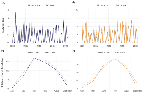
Figure 7 Observed and modeled number of hail days for the period of 2002–2012 (April to September) for the northern (a, c) and southern (b, d) domain. The gray lines are the observed number of hail days (POH ≥ 80 % over a minimum of 580 km² in the north and 499 km² in the south). The blue and orange lines are the number of hail days modeled from the ensemble predictions for the northern and southern models, respectively. Plots (a) and (b) show the absolute number of hail days per year, and (c) and (d) show the sum of hail days per month.

Generally, we see intra-annual and interannual variability in the skill of the statistical model in predicting hail days because some years and some months are predicted better than others (Figs. 7a, b and 8a, b). The overall correlation between the hail days per month and year of POH and the model is satisfactory, with 0.91 for the north and 0.87 for the south. Evaluating the model performance only for the years 2012–2022 yields slightly better values.

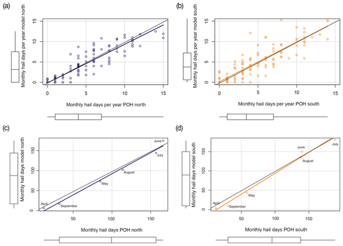
Figure 8 The observed number of hail days (POH ≥ 80 % over a minimum of 580 km² in the north and 499 km² in the south) plotted against the number of hail days modeled from the ensemble predictions for the northern domain (a, c) and southern domain (b, d) for the whole observational period of 2002–2022. Plots (a) and (b) show the absolute number of hail days per year, and (c) and (d) show the absolute sum of hail days per month. The black lines are the x=y lines, and the orange and blue lines are the fits to the orange and blue circles, respectively. Boxplots show the distributions of the samples.

Our model can reproduce the seasonal pattern in both domains well (Fig. 7c and d). The model captures the typical seasonal pattern with very few hail days at the beginning and end of the hail season and a peak during the warm summer months. The peak of hail days in the north (Fig. 7c) is in June and July but is more prominent in the southern domain (Fig. 7d) and appears mainly in July. The difference in peaks again justifies the use of two separate models to account for the monthly differences in hail frequency. In months with fewer hail days, the models tend to underpredict slightly in both domains (Fig. 8c and d). The correlation between the monthly sum of hail days of the model and the POH is 0.99 for the north and 0.98 for the south.

The ensemble prediction mean POD is 0.77 for the north and 0.61 for the south with an SR (1 − FAR) of 0.77 and 0.63, respectively. CSI is 0.60 and 0.44, and bias is 0.98 and 0.88, respectively. The POD, FAR, CSI, and bias are calculated by averaging the metric values of the test and validation datasets of the ensemble prediction; test and validation performance was very similar. The predictive skill of the ensemble prediction compares well with similar studies, such as those mentioned in Raupach et al. (2023a).

5 Analysis of the reconstructed time series

In this section, we present the reconstructed time series from the ensemble prediction and discuss its trends (Sect. 5.1), the drivers of these trends (Sect. 5.2), and changes in the seasonal cycle over time (Sect. 5.3). Finally, we compare our time series with qualitative damage data (Sect. 5.4).

5.1 Modeled long-term trends

Both domains exhibit a significant positive trend in yearly hail day occurrence, with a 45 % increase in modeled hail days in the northern domain and a 48 % increase in the southern domain comparing 1960–1989 to 1990–2019 (Fig. 9). Mann–Kendall's τ in the north is 0.355 with a p value of $\mathrm{4.70}\times {\mathrm{10}}^{-\mathrm{5}}$, and in the south τ is 0.369 with a p value of $\mathrm{2.43}\times {\mathrm{10}}^{-\mathrm{5}}$. The trend is slightly stronger in the south. The northern model estimates a mean of 18.87 hail days per year during the period of 1959–2022, with a minimum of 6 d in 1962 and 1980 and a maximum of 42 d in 2003 and 2018. In the south, the mean is 20.1 d, with a minimum of 6 d in 1984 and a maximum of 41 d in 2018. In the POH time series, 2003 and 2018 are also the years with the highest number of hail days. The mean number of yearly hail days for the 2002–2022 period is 24.1 d for the northern model and 24.4 d for the southern model. Both estimates are slightly lower than the POH average, with 24.1 hail days per year in the north and 25.3 hail days per year in the south. The variability of yearly or monthly sums of hail days increases over time, with higher variability in the last 2 decades (not shown).

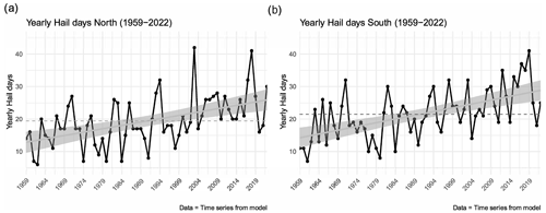
Figure 9 Modeled yearly aggregated hail days from 1959 to 2022 (black lines) for the northern (a) and southern (b) domains from the ensemble prediction. The dashed black lines represent the mean, and the solid gray lines with confidence intervals are the linear fits to the yearly hail days from 1959–2022.

It may be argued that deducing trends from ERA5 data-driven models provides biased results before 1979, when satellite data were first assimilated in ERA5. Therefore, we also performed the Mann–Kendall test limited to the period of 1979–2022; τ is 0.318 with a p value of $\mathrm{1.37}\times {\mathrm{10}}^{-\mathrm{5}}$ in the north and 0.463 with a p value of $\mathrm{2.87}\times {\mathrm{10}}^{-\mathrm{3}}$ in the south. This result means the trend is still positive and significant in both domains, although slightly less intense in the north and more pronounced in the south compared to the 1959–2022 period. This discrepancy is caused by the large interannual variability in both time series. The trends for both periods can be compared in Figs. 9 and C1.

5.2 Drivers of modeled trends

To investigate the factors driving the positive long-term trends in the models, we employed two techniques: partial Mann–Kendall tests and a detrending method proposed by Raupach et al. (2023b).

Using the Raupach et al. (2023b) approach, we assess the impact of individual model predictors on hail day trends by applying the models to data in which one of the predictors was detrended by removing the trend of the annual mean. We then performed Mann–Kendall tests to compare how the trend changed across the whole reconstructed time series from 1959–2022. To find which variable has the highest influence on the trend of each model, we compared τ values by exchanging one variable at a time with its detrended version for each model. For example, in the southern logistic regression model, detrending the LI resulted in a significant reduction in τ from 0.369 to 0.152, indicating a strong influence of LI on the positive trend. Similarly, detrending only KI reduced τ to 0.295, while τ only changed marginally when detrending other predictors. This result suggests that the positive trends in annual hail days in the southern logistic model are primarily explained by LI and to a lesser degree by KI.

Because τ is independent of the measurement scale, we can compare its values directly to find which predictors contribute most to the modeled trends. Across logistic regression models and GAMs for both domains, the positive trends in annual hail days were primarily driven by instability and moisture variables. To ensure the robustness of these results, we also performed partial Mann–Kendall analyses for each model and each model's predictors. We also performed partial Mann–Kendall tests on the ensemble predictions with a selection of parameters and found equal results. The tests again showed that in all models, the variables that contribute to the trends are primarily instability and moisture. The trend was never fully explained by a single variable but by a combination of both moisture and instability. This finding aligns with the connection known between convective instability and moisture availability.

Finally, we need to stress that the contribution of predictors to the trend depends on the importance of the predictors in the models. Additionally, the trend in the model always comes from the underlying trend in the model's predictors.

5.3 Change in the seasonal cycle over time

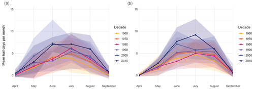
This section addresses the seasonal analysis of hail occurrence over time. The last 2 decades exhibit a marked increase in hail days per month, which is the strongest in May and June (Fig. 10, blue and purple curves). We excluded the years 1959 and 2020–2022 to ensure consistency in the number of years per decade. Although the monthly curves display considerable variability, their difference is not significant, and no systematic shift is evident, as illustrated by the cumulative distribution function (CDF) plots in Fig. C2. However, our analysis is confined to the months of April to September and cannot support any statements about potential changes in hail days preceding or following the period modeled here.

Figure 10 Panels (a) and (b) show the mean number of hail days per month per decade in colored lines with the uncertainty range. The 1960s include the years 1960–1969, the 1970s include the years 1970–1979, and so on. Panel (a) shows the northern domain and (b) the southern domain.

5.4 Plausibility check with historic hail data

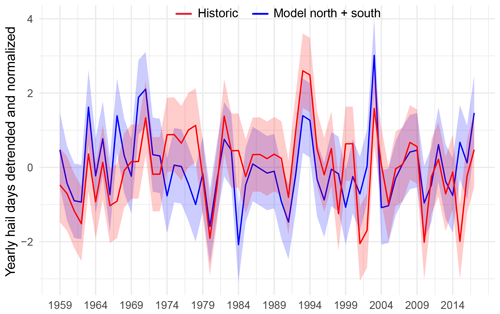
Validation of our time series and its trends with observational data was not possible due to the relatively short observational period. Nevertheless, we can conduct plausibility checks with qualitative hail information. As previously noted, these data do not enable any comparison of trends in the modeled time series with historical hail events, as the trends in damage are driven by changes in insurance coverage and exposure and vulnerability of crops. However, it is possible to compare interannual variability. Figure 11 shows the yearly sum of hail days extracted from the historical hail damage dataset in red from 1959 to 2017. The blue line is the yearly sum of both models. Both time series have been detrended and normalized. The correlation between the two time series is 0.43. We did not expect any better results because even for the period of 2012–2022, where we know that our model is closer to the true number of hail events than the historical information, some mismatch is evident. Of the 10 years with the highest number of hail days, 5 (2003, 1994, 1993, 1982, 1971) match, as do the 3 years with the lowest number of hail days (2010, 2005, 1980). Recall that we detrended both time series. When considering the non-detrended and non-normalized yearly time series, both have a similar standard deviation: 5.56 hail days for the model sum and 5.53 for the historical data.

Figure 11 The modeled number of hail days in blue (sum of northern and southern models) and the number of hail days derived from qualitative agricultural damage data in red (minimum five affected municipalities) for the 1959–2017 period. Both time series have been normalized and detrended.

6 Discussion

We evaluated ERA5 convective parameters and hail occurrence derived from Swiss radar data for the years 2012–2022 to develop a statistical reconstruction of past hail days in Switzerland. Our analysis has yielded several conclusions, among which the most important are discussed below.

6.1 Model predictor selection

The selection of predictors for the logistic regression models and GAMs needs to be discussed, in particular the absence of wind shear from the logistic regression models of both domains. When training our models, wind shear rarely appeared as a skillful predictor, and even when it did, it was not significant in the logistic regression models. Automated feature selection yielded similar results. We see three possible explanations for this. First, shear could also be indirectly represented by the variable v_500 (v wind component at 500 hPa; southern model) in the southern model.

Second, there is a nonlinear relationship between WS_06 (wind shear from 0 to 6 km) and the response in the GAM, which the logistic model struggles to fit. Additionally, neither v_500 nor the explicit wind shear variables show high feature importance in all models. This low feature importance has also been seen by Trefalt (2017) for Switzerland and by Mohr et al. (2015b) for Germany. A potential reason for this could be the prevalence of high-shear but low-CAPE conditions in our domains, which do not always lead to hail. Thus, the wind shear parameters may not be effective in distinguishing between hail days and non-hail days in a statistical model, since there is no statistically significant difference in the distributions of WS_06 and WS_36 on hail days vs. non-hail days in both domains.

Our third point is that high wind shear might be a less important hail model parameter in regions with complex terrain (Punge and Kunz, 2016). Although large shear values are required to form supercells, which are likely to produce hail, hail also develops in lower-shear environments (Schemm et al., 2016; Trefalt, 2017; Kumjian and Lombardo, 2020; Blair et al., 2021). In fact, Feldmann et al. (2023) found that only 10 % of severe hailstorms in Switzerland are supercell-type storms, and Schemm et al. (2016) find average lower-tropospheric shear values at hailstorm initiation locations in Switzerland of less than 10 m s⁻¹. Hail events in low-shear environments can be explained by proximity to mountain ranges, where environmental wind shear is increased by the interaction of the wind field with orography, which is often the case in the Alps (Trefalt, 2017; Kunz et al., 2018).

In such complex terrain, shear might be driven by local conditions, such as Alpine pumping, which are not resolved by ERA5's resolution. Alpine pumping arises from differential heating and cooling of air masses over mountains and plains, which drive daytime winds from plains to mountains and nighttime winds in the opposite direction (Lugauer and Winkler, 2005).

We also tested combinations of shear and CAPE, such as WMAXSHEAR, an important parameter for differentiating between severe and nonsevere weather (Brooks et al., 2003; Craven and Brooks, 2004; Kaltenböck et al., 2009; Púčik et al., 2015; Tuovinen et al., 2015), but for both domains, WMAXSHEAR was not selected in combination with other variables.

The combination of LI and TT including additional variables performed very well and overall better than CAPE and shear. This performance is why three of our models contain the combination of LI and TT. However, TT can be a problematic parameter for several reasons. First, composite parameters are hard to interpret in physical contexts because they combine multiple types of information. One does not know if TT is high because the lapse rates are favorable, because there is plenty of low-level moisture, or because there is a mix of both. This ambiguity is why it is hard to explain why the parameter worked well for our study. In addition, TT takes into account moisture from a single level (850 hPa) and is very sensitive to rapid changes in dew points with height. Consequently, TT can be a case-sensitive parameter that may reach high values in situations when there is no storm and thus create false alarms. This sensitivity is mitigated in the model by information obtained from other predictors.

We do not claim that the combination of LI and TT is better than, for example, CAPE and shear in forecasting individual hail cells or in differentiating between no hail, hail, and large hail. Rather, the specific combinations of approximately five variables in the statistical models worked best for the reconstruction of hail days in the Swiss study areas using the POH radar proxy and low-resolution ERA5 data. Our data-driven approach identified some less common indices; the statistical models leverage these indices effectively within the constraints of our data, and this statistical approach complements our physical understanding. However, our models should not be transferred to other periods or regions without additional verification. Forecasting applications are much better served by the operational COSMO and ICON weather forecast models than by ERA5.

The individual models suffer from rather high false alarm rates, and we were not able to increase the explained variance of the models above approximately 60 % for the northern models and 45 % for the southern models. Hence, the models still lack information for identifying when hail days occur. Notably, the models lack information about convection-triggering mechanisms. We tested including convective inhibition (CIN), but that variable was not a skillful predictor. Therefore, none of the models includes any representation of initiation processes.

This initiation problem is still a challenge for forecasting thunder- and hailstorms (Lock and Houston, 2014) and results in very high false alarm rates of statistical models in many studies. This problem could be addressed by using convective precipitation as a proxy for initiation or producing a model that computes probabilities of hail from the presence of lightning; an example of such a model is the additive regressive convective hazard model, AR-CHaMo, from Rädler et al. (2018) and Battaglioli et al. (2023a). However, even this model explains relatively low percentages of variance (approx. 30 %), implying the absence of information that cannot be captured by conventional convective parameters and coarse-resolution reanalysis data. This absence may be a motivation to look further into storm microphysics and, for instance, the location of the embryos in time and space during hail-favoring situations.

6.2 Comparison with other studies

Several studies have used logistic regressions or GAMs and daily data to model hail (López et al., 2007; Gascón et al., 2015; Mohr et al., 2015a, b; Rädler et al., 2018; Battaglioli et al., 2023a, b). Often, CAPE and shear are used as the main hail model predictors (e.g., Allen et al., 2015; Madonna et al., 2018; Czernecki et al., 2019; Battaglioli et al., 2023a). In our models, the combination of CAPE and shear was only significant in the southern GAM. For the logistic regression models, we found LI to be a better hail predictor than CAPE, which aligns with Kunz (2007), Mohr et al. (2015a, b), and Rädler et al. (2018). López et al. (2007) use TT and the wind at 500 hPa in their model for the Iberian Peninsula. Gascón et al. (2015) also used wind at 500 hPa. Unfortunately, we cannot directly compare the coefficients of their model to ours because of differences in data sources, resolution, and combination of model parameters. These differences must also be considered when comparing our model's performance to that of other studies.

To gauge the predictive capabilities of the models against those in related studies, we use the performance metrics of the ensemble predictions. Our models outperformed those mentioned in Raupach et al. (2023a) due to lower FAR and higher HSS values. Raupach et al. (2023a) mention HSS ranges from 0.1 to 0.4 compared to our models' HSS of 0.73 (north) and 0.55 (south). FAR ranges from 0.57 to 0.8 compared to 0.23 for the north and 0.35 for the south in our models. However, Raupach et al. (2023a) conducted their study over a much larger area encompassing diverse climate zones. Over our domains, hail is a comparatively frequent event with an a priori probability of approximately 15 % in the sample, which mitigates some of the statistical intricacies. Other studies have demonstrated comparable performance to ours, such as Battaglioli et al. (2023a) using ESWD hail reports and ERA5 data, López et al. (2007) using radar and radiosonde data, and Gascón et al. (2015) using severe-storm reports and Weather Research and Forecasting (WRF) vertical profiles.

6.3 Trends

Our modeled trends from the ensemble predictions align with the findings of Madonna et al. (2018), Rädler et al. (2018), and Battaglioli et al. (2023a). Madonna et al. (2018) reported an approximately 40 % increase in estimated hail days when comparing the periods of 1980–2001 and 2002–2014. Similarly, Rädler et al. (2018) found a 41 % relative increase in hail cases per year during 1979–2016 in western and central Europe. Battaglioli et al. (2023a) identified an 8 % per decade relative increase in hail hours in northern Italy and parts of southern Switzerland for the period of 1950–2022. In our study, we observe significant positive trends in both the northern and the southern domains, with a 45 % increase in modeled hail days in the northern domain and a 48 % increase in the southern domain comparing 1960–1989 to 1990–2019. This translates to a relative increase of 7.5 % and 7.9 % per decade, respectively. This trend can be attributed to an increase in hail-favoring environments in ERA5 in recent decades (Taszarek et al., 2021; Pilguj et al., 2022). Numerous studies have also identified positive trends in instability and moisture in ERA5 and rawinsonde data for Europe and parts of Switzerland (Mohr and Kunz, 2013; Rädler et al., 2018, 2019).

Our modeled trends in hail occurrence are subject to several limitations. First, POH serves as the “truth”, but POH is an indirect observation of hail and does not perfectly reflect the presence of hail on the ground (Kopp et al., 2024). Additionally, the quality of ERA5 data changes over time as more data are assimilated into the reanalysis. The study of Pilguj et al. (2022) comparing ERA5 trends to those extracted from rawinsonde data showed that the reliability of ERA5 has increased in the last 4 decades, implying higher confidence in the positive trends for the 1979–2022 period.

Finally, we want to highlight a limitation in the explanation of our trends. Within our models, the positive trends in annual hail day occurrences are driven by moisture and instability predictors (see Sect. 5.1). We can only quantify the effects of variables that are selected as predictors in the models. Other factors influencing hail occurrence and trends, such as temperature, could still play an important role due to the strong link between temperature, moisture availability, and convective instability.

We assume that the relationship modeled between the predictors and the occurrence of hail is stationary in the period that we investigate. The relationship might break down in a warmer climate, such as with drier summer soils, and the models should not be directly applied to climate change simulations. Studies using Coupled Model Intercomparison Project data have also shown that we could see reductions in relative humidity (RH) but increases in absolute humidity, involving lower RH but higher dew points (Hoogewind et al., 2017; Chen et al., 2020) over Europe. Despite larger CAPE, the process of convective development may become more difficult due to lower mid-level RH, which leads to a higher lifting condensation level, a higher level of free convection, and thus more negative buoyancy and larger CIN (Hoogewind et al., 2017; Chen et al., 2020; Taszarek et al., 2021). The rise in the freezing level induced by lower- to mid-tropospheric warming could result in hail melting before reaching the ground (Dessens et al., 2015; Raupach et al., 2023a).

7 Conclusion and outlook

We present a new multidecadal daily hail time series for northern and southern Switzerland from 1959 to 2022, reconstructed from a POH radar hail proxy and ERA5 environmental predictors with statistical models. We built an ensemble prediction from a multiple logistic regression model and a logistic GAM for northern Switzerland and southern Switzerland. Model development included the selection of the most hail-relevant predictors based on multiple performance metrics, residual analysis, and multicollinearity and finding the best model settings. Seasonality is explicitly modeled by a categorical factor for the month in each model. Including the month factor led to a reduction in systematic biases in the residuals, as well as to an improvement in predictive skills. The hail time series was used to analyze long-term trends and changes in frequency, seasonality, and the variability of model-derived Swiss hailstorms in the past few decades.

The final ensemble model reproduces the interannual variability and seasonality of hail radar proxies well. The reconstructed hail time series shows a significant positive trend in the number of hail days per year in both domains from 1959 to 2022. In the south the trend is 7.5 % per decade. The trend is also significant and positive for the period of 1979–2022. The trend is mainly driven by the instability and moisture predictors in all models. The increase in hail days in the last 2 decades is the strongest in May and June. However, the seasonal cycle shows no clear shift towards an earlier start or earlier end, and differences in monthly distributions across decades are not significant. We compared our time series to a historical agricultural insurance data archive. We found agreement in the weakest and strongest hail years and similar interannual variability.

The main purpose of this study is to offer a framework to study intra-annual variability, trends, and past changes in the seasonality of Swiss hail occurrence without long-term direct hail observations. We will use this time series to study local and remote drivers of the intra-annual and interannual variability of Swiss hail. These drivers include sea surface temperature (Jeong et al., 2020; Cheng et al., 2022), soil moisture anomalies (Taylor, 2015; Gaal and Kinter, 2021), and sea ice and snow cover (Wiese, 1924; Budikova, 2009). Similarly, it would be interesting to see whether these large-scale variables are related to specific circulation anomalies or synoptic configurations (Schemm et al., 2016; Piper and Kunz, 2017; Rohrer et al., 2019). This question will be the subject of future work.

Appendix A: Calculation of model performance metrics

The Akaike information criterion (AIC; Akaike, 1974) and the Bayesian information criterion (BIC; Schwarz, 1978) were calculated with the R stats package. The AIC is defined as $\mathrm{AIC}=-\mathrm{2}\times \ln \left(L\right)+k\times n_{\mathrm{par}},$ where ln (L) is the logarithm of the maximum likelihood of the estimated model, k=2, and n_par is the number of fitted model parameters. For glm, $-\mathrm{2}\times \ln \left(L\right)$ is the deviance. Using k=log (n) provides the BIC instead, where n is the number of observations. The variance inflation factor (VIF) was also calculated in R by ${\mathrm{VIF}}_i=\mathrm{1}/\left(\mathrm{1}\mathrm{-}{R}_i^{\mathrm{2}}\right)$, where $R_i^{\mathrm{2}}$ is the coefficient of determination obtained when regressing the ith predictor on the others.

Figure A1 represents the ensemble predictions' skill in a performance diagram showing the POD (left y axis), SR (lower x axis), CSI (labeled solid contours), and bias scores (labeled dashed lines) (diagram by Roebber, 2009). A perfect prediction would lie in the top-right corner of the performance space, meaning all metrics approach unity, achieving 100 % correct predictions. The nearer the predictions are to the lower-left corner, the more biased they are, and the more false positives or misses a model produces.

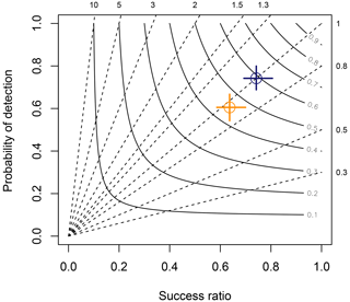
Figure A1 Performance diagram summarizing the POD, SR, bias, and CSI of each model. The orange cross shows the performance skill of the south and the blue cross that of the north. The crosslines indicate the confidence interval, calculated from bootstrapping. The circles highlight the mean value. The dashed lines represent bias scores with labels on the outward extension of the line. Labeled solid contours are the CSI.

Table A1 Equations and limits for performance metrics that were used to find the best hail models. Performance metrics were calculated from the corresponding contingency tables. TP represents the true positives, FP the false positives, FN the false negatives, and TN the true negatives.

Appendix B: Model coefficients

B1 Logistic models

Table B1 Coefficients, standard errors, z values, and p values of all covariates of the logistic regression models for north and south. Positive signs indicate a positive relationship of the quantitative predictors with modeled hail occurrence and vice versa. Asterisks indicate significance levels of the p values: ^* 0.01, ${}^{**}$ 0.001, and ${}^{***}$ 0.000.

B2 GAMs

To examine whether we obey the assumptions necessary for logistic regression, we also checked for extreme outliers and for the linear relationship between the explanatory variables x_n and the logit of the response variable y. Some variables did not have a perfect linear relationship, such as CAPE, which is probably one reason why it was not chosen as a predictor for the final logistic regression models. We also build GAMs to allow for nonlinear relationships and interactions that might be poorly fitted in the logistic regression models (see Sect. 4.2).

Table B2 Coefficients, standard errors, z values, and p values of all nonparametric covariates of the GAMs for north and south. Positive signs indicate a positive relationship of the quantitative predictors with modeled hail occurrence and vice versa. Asterisks indicate significance levels of the p values: ^* 0.01, ${}^{**}$ 0.001, and ${}^{***}$ 0.000. Other nonparametric terms are found in Table B3.

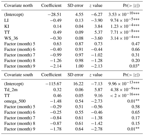
Table B3 Significance of nonparametric smooth terms in the GAM for the north and the GAM for the south. Edf is the effective degree of freedom, ref. df represents the residual degree of freedom, and chi. sq. is the chi-square statistics. Asterisks indicate significance levels of the p values: ^* 0.01, ${}^{**}$ 0.001, and ${}^{***}$ 0.000.

Appendix C: Additional figures

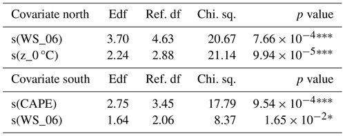
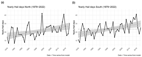
Figure C1 Similar to Fig. 9 but for the period of 1979–2022. The linear fit is calculated for the yearly hail days from 1979–2022.

Figure C2 Cumulative distribution functions of the number of hail days per week per decade (colored lines). Panel (a) shows the northern domain and (b) the southern domain.