InSAR-informed in situ monitoring for deep-seated landslides: insights from El Forn (Andorra)

Monitoring deep-seated landslides via borehole instrumentation can be an expensive and labor-intensive task. This work focuses on assessing the fidelity of interferometric synthetic-aperture radar (InSAR) as it relates to sub-surface ground motion monitoring, as well as understanding uncertainty in modeling active landslide displacement for the case study of the in situ monitored deep-seated El Forn landslide in Canillo, Andorra. We used the available Sentinel-1 data to create a velocity map from deformation time series from 2019–2021. We investigated the performance of InSAR data from the recently launched European Ground Motion Service (EGMS) platform and the Alaska Satellite Facility (ASF) On Demand InSAR processing tools in a time series comparison of displacement in the direction of landslide motion with in situ borehole-based measurements from 2019–2021, suggesting that ground motion detected through InSAR can be used in tandem with field monitoring to provide optimal information with minimum in situ deployment. While identification of active landslides may be possible via the use of the high-accuracy data processed through the EGMS platform, the intent and purpose of this work are the assessment of InSAR as a monitoring tool. Based on that, geospatial interpolation with statistical analysis was conducted to better understand the necessary number of in situ observations needed to lower error in a remote sensing re-creation of ground motion over the entirety of a landslide, suggesting between 20–25 total observations provide the optimal normalized root mean square error for an ordinarily kriged model of the El Forn landslide surface.

1 Introduction

Deep-seated landslides represent one of the most devastating natural hazards on earth, many creeping at inappreciable velocities over several years before suddenly collapsing, usually with catastrophic velocities (Smalley, 1978; Voight, 1988). While there is a range of landslide sizes, several deep-seated landslides include sizable earth slides involving millions of cubic meters of soil moving as a rigid block on top of a deep (below the roots of the trees and the groundwater level) basal layer of heavily deformed minerals (Petley and Allison, 1997; Frattini and Crosta, 2013). Their collapse is usually very sudden, happening within minutes and without a clear warning, reaching high velocities, as high as the 20 m s⁻¹ reported at the 1963 Vaiont landslide in Italy (Voight, 1988; Smalley, 1978; Veveakis et al., 2007). The catastrophic and fast collapse of this kind of landslide makes the evacuation of the area that could be affected a cumbersome task, thereby increasing the risk of fatalities and infrastructure damage (Reid, 1994, 2015; Guzzetti, 2000). Moreover, the complex physical nature of the landslides induces high uncertainty in the number of in situ observations required for a high-fidelity monitoring system. That, in combination with the challenging and expensive methods of in situ monitoring, makes the development of reliable, data-driven, early warning systems (or tools/protocols to stop the acceleration of the landslide) an appealing proposition.

Before the use of satellites, initial approaches in predicting the catastrophic collapse of a landslide relied on physical access to the area with in situ (extensometer) or ex situ (lidar, UAV) displacement data, whereby an assessment is made using the inverse-velocity method (Jaboyedoff et al., 2012; Saito, 1969; Carlà et al., 2017; Zhou et al., 2020). Considerable work has since been done in developing remote sensing methods for landslide identification (Handwerger et al., 2019; Zhong et al., 2020; Mohan et al., 2020; Casagli et al., 2023; Chi et al., 2002; Zhao and Lu, 2018) and creating predictive models of deep-seated landslides based on identifying different mechanisms involved as triggering factors of the acceleration like rainfall (Reid, 1994), temperature (Mitchell et al., 1968; Veveakis et al., 2007), and chemical alterations (Hueckel and Pellegrini, 2002). Both developments are now at a stage where they can be used in conjunction with high-fidelity field data (piezometers, extensometers, and thermometers) to obtain forecasting and mitigation protocols (Seguí and Veveakis, 2021, 2022). However, the installation of such in situ instrumentation is a costly operation, requiring the transportation of heavy equipment often in remote areas and the installation of sensors in deep boreholes that cannot be deployed readily across the world.

To overcome these constraints, the use of remote sensing has become a more available tool for landslide monitoring over the last several decades. Several techniques for mapping and assessing slope movements have been developed, thus allowing for a more reliable and fast investigation (Cigna et al., 2013; Fiorucci et al., 2011; Guzzetti et al., 2009; Michoud et al., 2012). Among the remote sensing options, the use of synthetic-aperture radar (SAR) sensors has gained significant popularity for measuring surface deformations and constructing their time series, since this approach requires no access to the site to install borehole instrumentation or handle UAV and lidar devices. Remote monitoring approaches for deep-seated landslides are limited by their frequent inability to provide information for the body of the landslide when the moving mass is deep-seated in steep valleys or densely vegetated mountain ranges, as well as their nature as surface-only measurements. This work builds on the existing literature concerning the assessment of how reliable remote surface measurement tools could be for deep-seated landslides (Bayer et al., 2017; Fobert et al., 2021; Bellotti et al., 2014; Casagli et al., 2023; S and Kanungo, 2004; Lissak et al., 2020; Scaioni et al., 2014; Wang et al., 2019), providing a case study from the El Forn landslide in terms of the data quality needed to identify and monitor a landslide and extending this body of literature using interferometric synthetic-aperture radar (InSAR) data to decide the minimum number of in situ observations needed for that.

2 Material and methods

2.1 Description of the El Forn landslide and in situ data

The El Forn landslide is a large deep-seated landslide located southeast of the town of Canillo, Andorra, nestled in the Pyrenees (see Fig. 1) that is triggered by snowmelt and season rainfall that collect into an aquifer located below the sliding surface. This landslide has a sliding mass of approximately 300 Mm³ that creeps at an average rate of 1.2 cm yr⁻¹ (Seguí and Veveakis, 2021). Within the main sliding mass of the landslide, there is a faster-moving lobe (Cal Ponet–Cal Borronet lobe) that slides at a maximum velocity of 2–4 cm yr⁻¹ (EuroConsult, 2023; Seguí and Veveakis, 2021; Zhao and Lu, 2018). At present, this lobe is equipped with 12 boreholes dispersed between the top and bottom of the landslide collecting continuous in situ data. However, S10 is the only continuously monitored borehole on the landslide, with measurements every 20 min. Other boreholes are monitored via analog non-continuous measurements (irregularly, approximately once per month), which is why we chose to work exclusively with S10. It is important to note that, while there are available analog data over the landslide, only one point is a viable option for comparison with InSAR, given the no-snow period of 2019. In order to not reduce the fidelity of the continuous time series from S10, the authors choose to not include these data in the body of this text. The authors have made these data available upon request.

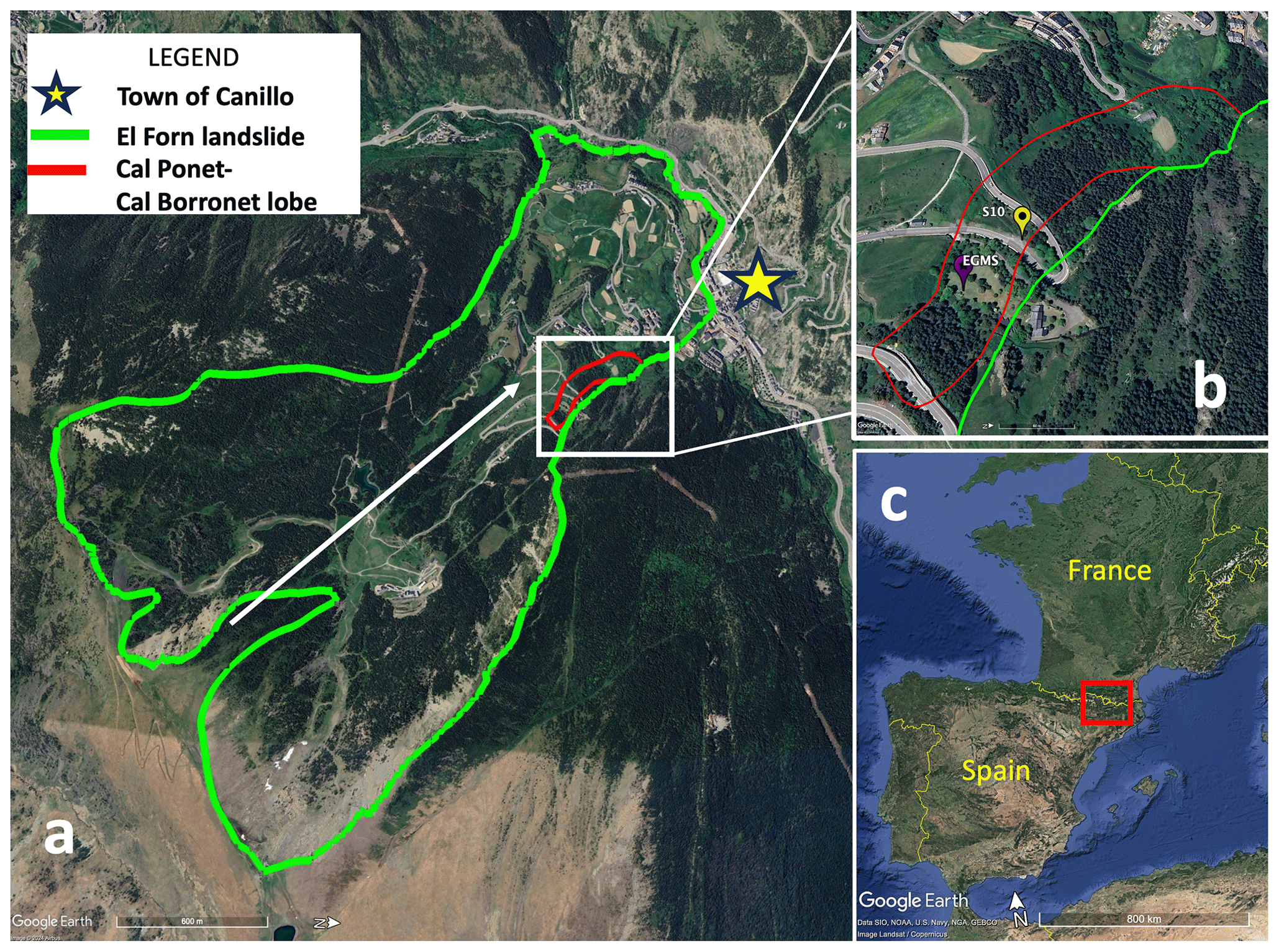
Figure 1 (a) Overview of the El Forn landslide with the Cal Ponet–Cal Borronet lobe, noted with the EGMS observation (see Sect. 2.2.2) and S10 borehole location. White arrow shows the direction of the landslide into the town of Canillo, marked with a star. (b) Cal Ponet–Cal Borronet lobe with the S10 borehole. (c) Localization of the landslide in Andorra. Images © 2024 Airbus.

The sliding surface is located at 29 m depth, and the landslide moves as a rigid block (Seguí and Veveakis, 2021) on top of it, creeping into the town of Canillo, as shown in Fig. 1, with the periods of greatest acceleration during the no-snow periods (May–August) each year. The shear band is comprised of 80 % Silurian shales rich in phyllosilicates (muscovite, paragonite, and chlorite) and 20 % quartz (Seguí et al., 2020). A more detailed explanation of the geological makeup of the shear band can be found in Seguí et al. (2020). The terrain of the landslide can be seen in Fig. 1.

The primary instrumentation and data considered in this study are housed within the S10 borehole, noted as the yellow marker in Fig. 1. Data from S10 are sampled continuously every 20 min via instrumentation including an extensometer, three piezometers, and a thermometer within the shear band, which measure horizontal displacement, water pressure, and temperature changes in the material, respectively. The data considered in this study for El Forn are displacement measurements gathered from the extensometer. Detailed information about the location of S10 and the depth profile of the landslide with S10 borehole readings can be found in Seguí and Veveakis (2021).

2.2 Remote data collection and processing

One of the key objectives of this work is to compare InSAR to sub-surface ground measurements. This is achieved through interferograms obtained by Sentinel-1A and Sentinel-1B over a period of 6 months in 2019 with a 6 d acquisition interval. It is important to note that the landslide was arrested at the end of 2019, so 2019 remains the year of focus for the intent and purpose of this work. Additionally, a 6-month InSAR time interval is chosen in order to avoid snow cover seasons on El Forn since backscatter from snow cover makes use of InSAR particularly difficult due to low coherence (Kumar and Venkataraman, 2011; PBC, 2022). Interferograms are then processed to obtain displacement time series over the landslide's surface using two different approaches.

1. A high-precision (fine-spatial-resolution), low-accuracy (noisy) approach was employed, whereby Sentinel-1 data are retrieved and pre-processed with a low coherence threshold to obtain high-spatial-resolution (40 m×40 m grid) displacement data so that geospatial analysis can be conducted to determine the minimum number and location of observations required for landslide monitoring and reconstruction with quantified uncertainty. This approach was deployed using the Alaska Satellite Facility (ASF) On Demand InSAR processing tools from the Vertex platform and will be hereinafter referred to as ASF.

2. A low-precision (sparse-spatial-resolution), high-accuracy (de-noised) approach was employed, whereby Sentinel-1 data are filtered to reduce the noise so that landslide identification can be achieved from high-accuracy data on a 100 m×100 m grid. This approach was performed via immediate download through the newly launched European Ground Motion Service (EGMS) platform from Copernicus (EGM, 2023) and will be hereinafter referred to as EGMS.

Note that the SAR imagery for both the data retrieved via the ASF On Demand InSAR processing tools and the Copernicus EGMS portal was taken from the Sentinel-1A and Sentinel-1B satellites on a descending track with a 270° angle of incidence from the vertical. Using the slope of the ground at S10, the data for the EGMS displacement and ASF–MintPy (Miami INsar Time-Series software in Python) readings were translated into the displacement along the direction of the landslide movement so they could be compared to S10's strain gauge readings.

While displacement data from EGMS are readily available, data retrieval from ASF requires a more hands-on approach, going through a short baseline subset pre-processing step via ASF On Demand InSAR processing tools, followed by an interferogram time series inversion via MintPy that allows us to generate mean deformation velocity maps and deformation time series (Berardino et al., 2002; Handwerger et al., 2019; Yunjun et al., 2019). Subsequent displacement data from this time series inversion, alongside displacement data pulled from the EGMS platform, are compared with in situ displacement data from S10 to understand the correlation between InSAR and in situ data. The other key objective of this work is to understand how InSAR can be used for a general uncertainty quantification for planning future borehole placement, should the first objective prove InSAR can be correlated with sub-surface measurements. This will be done via iterative ordinary kriging, with the normalized root mean square error (RMSE) being used as the statistical parameter of interest for confidence. The next paragraphs outline the technical details of data retrieval and processing for each of these approaches.

2.2.1 ASF InSAR data retrieval and time series inversion

Open-access descending-track SAR acquisitions from the Sentinel-1 C-band (radar wavelength of approximately 5.66 cm) were pulled from the Alaska Satellite Facility (ASF) Vertex portal and processed automatically through this portal via the Advanced Rapid Imaging Analysis (ARIA) natural hazards project (Bekaert et al., 2019).

InSAR data retrieved for the purposes of this work were retrieved by selecting single-look complex (SLC) scenes with a beam mode of interferometric wide (IW) covering the El Forn landslide. Using the Alaska Satellite Facility On Demand tool, scenes were selected and pre-processed using the short baseline subset (SBAS) tool, making it easier to order the best interferograms for SBAS. However, MintPy's default time series tool was ultimately used. From there, all 619 interferograms covering El Forn were downloaded via a Python script from the ASF Vertex platform. Interferograms with visible discontinuities were manually identified once downloaded and removed from the stack for time series analysis. From there, the ASF Hybrid Pluggable Processing Pipeline (HyP3) service allowed for each interferogram to be clipped to the same size of overlap to standardize each interferogram. Using MintPy (see Yunjun et al., 2019, for more information on the time series inversion process), clipped interferograms were then inverted to create a deformation time series using a weighted least-squares inversion with a coherence threshold value of 0.4. This approach creates velocity and deformation maps on a 40 m×40 m grid, as shown in Fig. 2a. It is to be noted that the low coherence threshold used provides high-spatial-resolution maps that can be used for geospatial analysis; however this increased resolution is accompanied by increased noise, which makes landslide identification cumbersome, as seen in Fig. 2a and discussed in Results. For this reason, a second approach is pursued in parallel, focusing on the accuracy of the data as detailed below.

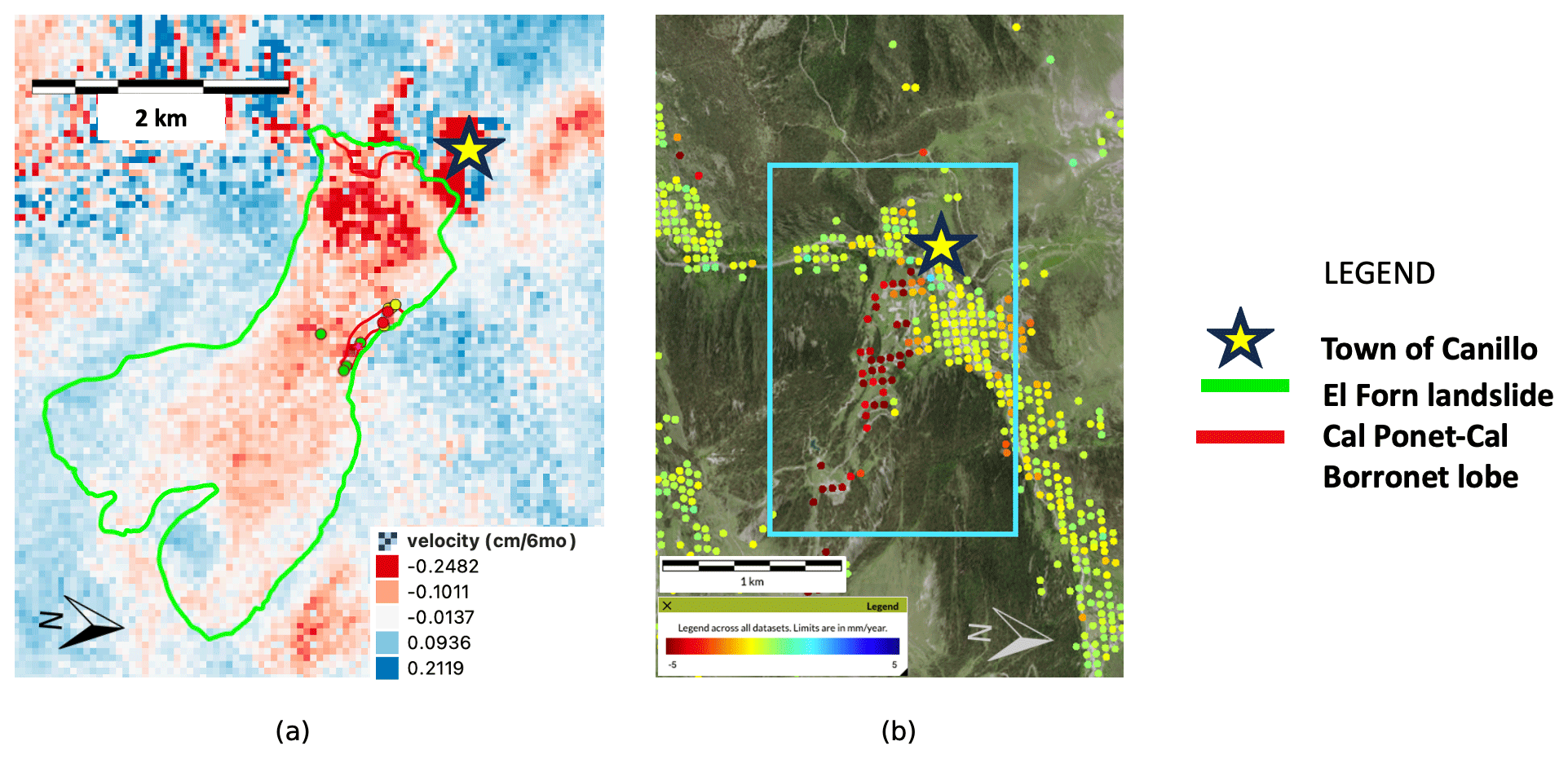
Figure 2 Depiction of the El Forn landslide using InSAR. (a) Overview of the velocity of the El Forn landslide using data retrieved and inverted using ASF against the field observation of the landslide boundary (green line). Colored dots indicative of total borehole locations, delineated by color due to separate monitoring agencies in partnership with the government of Andorra. (b) InSAR detection of the El Forn landslide by the Copernicus EGMS platform (highlighted in blue; retrieved on 28 September 2023), indicative of the possible use of EGMS as a tool for active landslide detection.

2.2.2 EGMS InSAR data retrieval and time series inversion

A second set of InSAR data was taken from the European Union's Copernicus project via the European Ground Motion Service (EGMS) portal, available for immediate retrieval as vertical and east–west displacement series per point. This platform provides already processed displacement data over parts of El Forn at a grid of around 100 m×100 m resolution as seen in Fig. 2b, with the location of data points apparent as dots over the topography of the El Forn landslide.

As already mentioned, there are key differences between the data retrieved via the ASF On Demand InSAR processing tools and the data retrieved from the EGMS portal for the intent and purpose of this work – the key trade-off being between precision and accuracy. More specifically, the ASF On Demand data inverted via MintPy used a minimum coherence threshold of 0.4, whereas EGMS Ortho data only visualized individual measurement points greater than or equal to 0.8. It is to be noted that the EGMS results could have also been obtained by applying a higher threshold value to the ASF approach, making the choice between the tool used scientifically immaterial. The reasons for utilizing both in parallel are the ability to showcase and cross-validate the two approaches.

2.3 Spatial interpolation and ordinary kriging

Ordinary kriging was conducted by first creating a grid of x and y coordinates and corresponding velocity values at these points. Distances between the random observations and each individual grid point were calculated such that

$$\begin{array}{}\text{(1)}& d_{\mathrm{1}}=\sqrt{(x_{\mathrm{g}}-x_{\text{obs}}^T{)}^{\mathrm{2}}+(y_{\mathrm{g}}-y_{\text{obs}}^T{)}^{\mathrm{2}}},\end{array}$$

where x_g and y_g are the grid coordinates and x_obs and y_obs are the random observation coordinates. The covariance matrix was determined using the range τ and variance σ² from the semivariogram such that

$$\begin{array}{}\text{(2)}& \mathbf{C}={\mathit{\sigma }}^{\mathrm{2}}\left(e^{(-d_{\mathrm{1}}/\mathit{\tau }{)}^T}\right).\end{array}$$

The Euclidean distances between the random observations and each other were calculated, as well as the corresponding covariance matrix Σ, such that

$$\begin{array}{}\text{(3)}& {\displaystyle }{d}_{\mathrm{2}}=\sqrt{(x_{\text{obs}}-x_{\text{obs}}^T{)}^{\mathrm{2}}+(y_{\text{obs}}-y_{\text{obs}}^T{)}^{\mathrm{2}}},\text{(4)}& {\displaystyle }\mathbf{\Sigma }={\mathit{\sigma }}^{\mathrm{2}}\left(e^{(-d_{\mathrm{2}}/\mathit{\tau }{)}^T}\right).\end{array}$$

The covariance matrices were appended into two matrices that would be used Lagrange multipliers, matrices Σ^′ and C^′, respectively. The weights were calculated by solving the linear equations created by the Σ and C matrices. From there, we calculate predictions Z^* by taking the velocity values at the random observations z_t, multiplying them by the corresponding weights W such that

$$\begin{array}{}\text{(5)}& {\mathbf{Z}}^{*}=\mathbf{\Sigma }(\mathbf{W}\cdot z_t).\end{array}$$

The mean square error is then solved such that

$$\begin{array}{}\text{(6)}& \text{MSE}={\mathit{\sigma }}^{\mathrm{2}}-\mathbf{\Sigma }(W\cdot {\mathbf{C}}^{\prime })-\mathbf{W}.\end{array}$$

As a result, fidelity was assessed via the root mean square error ($\text{RMSE}=\sqrt{\text{MSE}}$) of a kriged landslide surface via random sampling without replacement per iteration.

3 Results

3.1 Landslide identification

As previously noted, ASF and EGMS data showcase a key trade-off between precision and accuracy for the purposes of landslide monitoring. Figure 2a demonstrates that with a lower coherence value, more, albeit noisy, data are available. In a separate vein, the EGMS data (pictured in Fig. 2b) demonstrate the utility of an increased coherence value in reducing noise and producing high-accuracy data usable for landslide detection.

3.2 Correlating InSAR with in situ data for seasonal ground motion

Upon data retrieval, both ASF and EGMS InSAR displacements were compared along the direction of sliding in situ strain gauge data from the S10 borehole in order to understand the fidelity of InSAR in monitoring sub-surface ground motion. This direct comparison of InSAR readings from ASF and EGMS over the S10 borehole can be seen in Fig. 3. Retrieval of InSAR displacement data from EGMS required manual comparison of a couple of neighboring points with S10's in situ data in order to find points with a signal strong enough to use for comparison since there was no individual measurement point at the location of S10 after the increased threshold was applied (see Fig. 1).

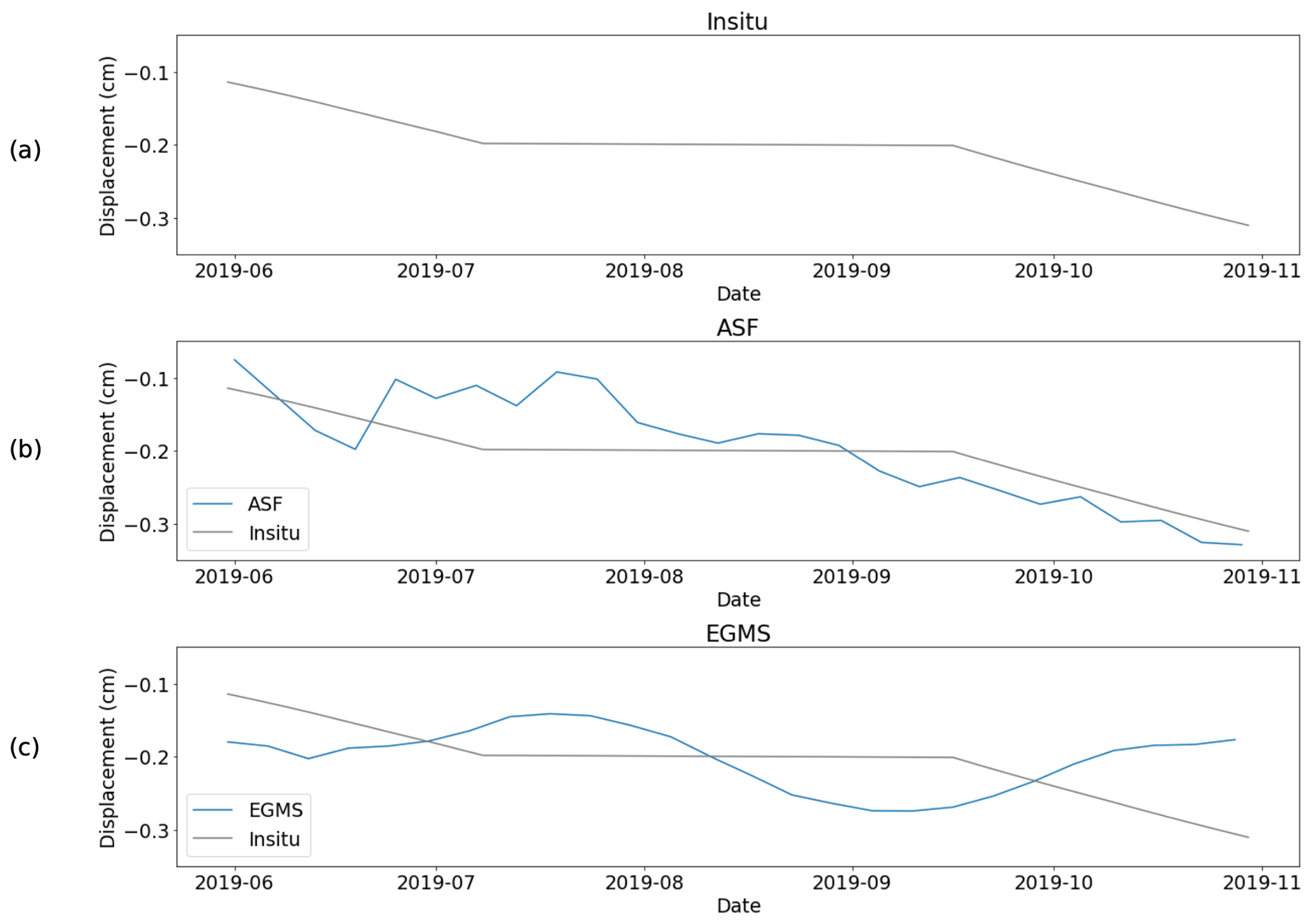
Figure 3 Comparison of in situ displacement data with displacement data retrieved via EGMS and ASF On Demand processing tools. (a) In situ displacement readings from the S10 borehole. (b) The 7 d cumulative moving average of InSAR displacement readings over S10 with data retrieved via ASF On Demand processing tools. (c) The 7 d cumulative moving average of InSAR displacement readings with data retrieved from EGMS.

Indeed, the increased sparsity from EGMS resulted in a lack of precision of the individual measurement points in comparison with in situ measurements, as seen in Fig. 3c, as compared to data retrieved via ASF On Demand tools (as seen in Fig. 3b). Since data for the exact location of the S10 borehole on the landslide were not immediately available on the EGMS platform, two coordinates neighboring the WGS84 coordinate of S10 were pulled and compared to the S10 data and InSAR data. Heterogeneity within the landslide prevented selecting just one point as close to the S10 point as possible without properly examining other neighbors. Figure 1 details which point was examined, with “EGMS” being the point in the EGMS database that was ultimately used because of its close alignment with S10's raw displacement data. Figure 3 directly compares data retrieved with ASF On Demand processing tools (and inverted via MintPy) and EGMS with in situ displacement measurements. We observe that while InSAR displacement measurements pulled from EGMS are helpful in detection, the higher accuracy creates data that lack the precision necessary for in situ comparison.

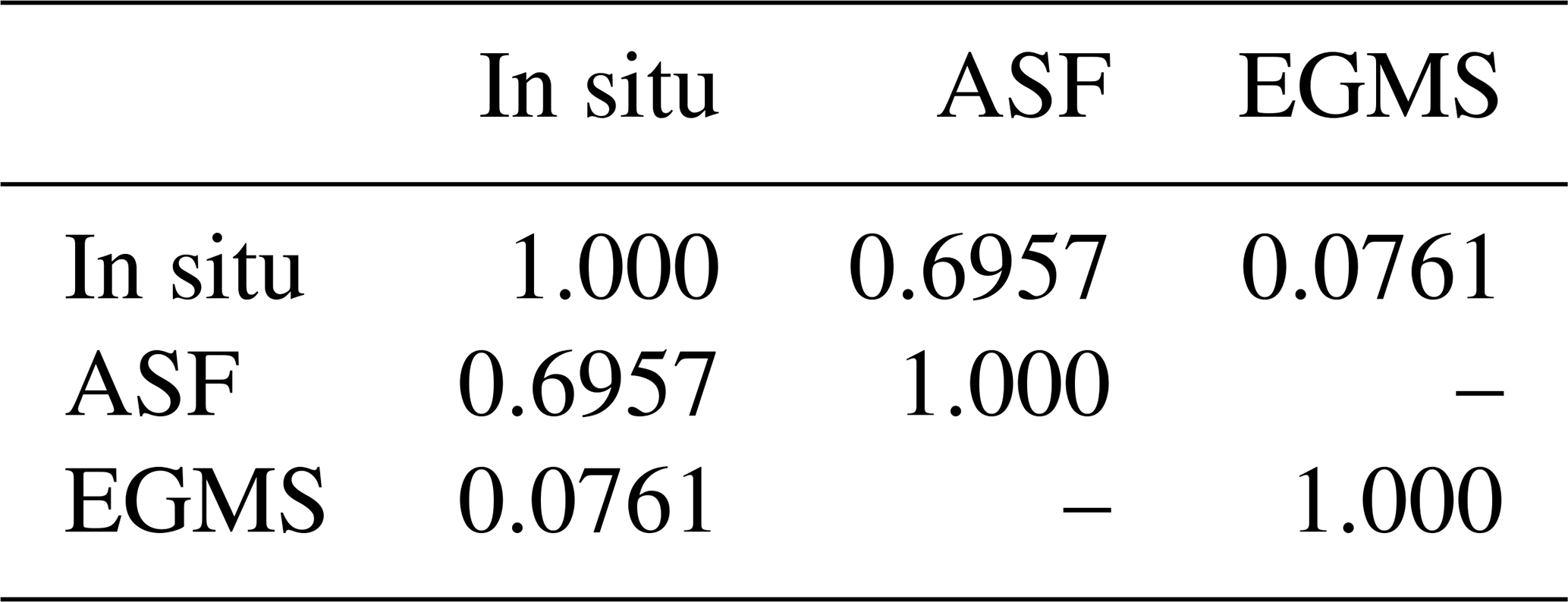
In order to justify this claim and quantify the performance of the two approaches in time, a measure of linear independence (correlation) was conducted with data with in situ measurements from EGMS and ASF, respectively. The equation used for the calculation of the correlation coefficient ρ(A,B) of datasets A (in this case EGMS or ASF) and B (in this case the in situ data) is

$$\begin{array}{}\text{(7)}& \mathit{\rho }(A,B)={\displaystyle \frac{\mathrm{1}}{N-\mathrm{1}}}\sum _{i=\mathrm{1}}^N\left({\displaystyle \frac{A_i-{\mathit{\mu }}_A}{{\mathit{\sigma }}_A}}\right)\left({\displaystyle \frac{B_i-{\mathit{\mu }}_B}{{\mathit{\sigma }}_B}}\right),\end{array}$$

where μ and σ are the mean and standard deviation of the datasets, respectively. The results of the performance of ASF and EGMS against the in situ data are detailed in Table 1, where we see that the ASF dataset ($\mathit{\rho }(\text{ASF},\text{in situ})=\mathrm{0.6957}$) performs considerably better against in situ data than EGMS ($\mathit{\rho }(\text{EGMS},\text{in situ})=\mathrm{0.0761}$). This is presumably due to the spatial heterogeneity of the landslide's displacement around the point of measurement, which is not exactly on S10 (see Fig. 1), and is not reflective of the overall quality of the EGMS data.

Table 1 Comparison of correlation coefficients (Eq. 7) of displacement data retrieved from ASF and EGMS with in situ measurements.

3.3 Ordinary kriging: determining necessary number of remote observations

Having shown the correlation between ASF and in situ measurements in the previous section, we move forward with the densely populated ASF mapping to carry out ordinary kriging. In order to best understand how many observations (i.e., boreholes) impact the ability to remotely model ground motion of a deep-seated landslide, 200 iterations of randomly selected samples (with sizes ranging from 5–100 points) along the main landslide surface were selected and had ordinary kriging performed on them to assess the RMSE in predicting ground motion over the surface of the landslide, with summaries of RMSE for each number of iterations visible in the box-and-whisker plot in Fig. 4. Similarly, single-iteration ordinary kriging was conducted over the sliding mass to assess how various sample sizes (ranging from 10–2000) were involved in re-creating velocities of the sliding mass and where possible areas of interest for further investigation were.

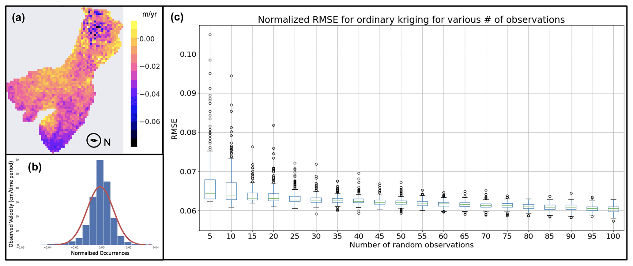
Figure 4 (a) InSAR velocity map of the 2019 snow-free period in Andorra via ASF-processed InSAR. (b) Uniform distribution probability density function (red line) and occurrence histogram (blue) of velocities pulled from panel (a). (c) Boxplot of normalized RMSE of 200 iterations for various numbers of random observations of velocities from panel (a) pulled from the uniform distribution in panel (b).

More specifically, 200 iterations were conducted per number of random observations of the average velocity in 2019 (pulled from a uniform distribution, as seen in Fig. 4b), results of which can be seen in Fig. 4c. Figure 4c, the diagram of the normalized root mean square error (RMSE), indicates a marked drop in the interquartile range (IQR) between 20 and 25 observations. Also important to notice is that the range of outliers is significantly lower, starting from n=25 observations and going forward. Note that the dots outside of the whiskers are outliers, meaning they lie outside of the whiskers defined by $Q\mathrm{1}-\mathrm{1.5}\cdot \text{IQR}$ and $Q\mathrm{3}+\mathrm{1.5}\cdot \text{IQR}$.

Figure 5 reflects how n samples re-create the average landslide velocity movement over the no-snow periods in 2019 in the line of sight (LOS) and the fidelity (RMSE) of doing so. For example, n=30 random samples re-create certain parts of the landslide better than others for one iteration. Figure 5 shows the evolution of how increased random samples that go through the process of ordinary kriging then re-create certain parts of the landslide surface faster or better than others. In the case of n=30, the top and bottom of the landslide are better developed than the middle of the landslide, which indicates where further investigation may be necessary. More specifically, the center of the landslide is the least developed throughout the iterations of ordinary kriging – for modeling purposes then, further investigation would be required on this part of the sliding mass (either further instrumentation or a more narrow scope of InSAR).

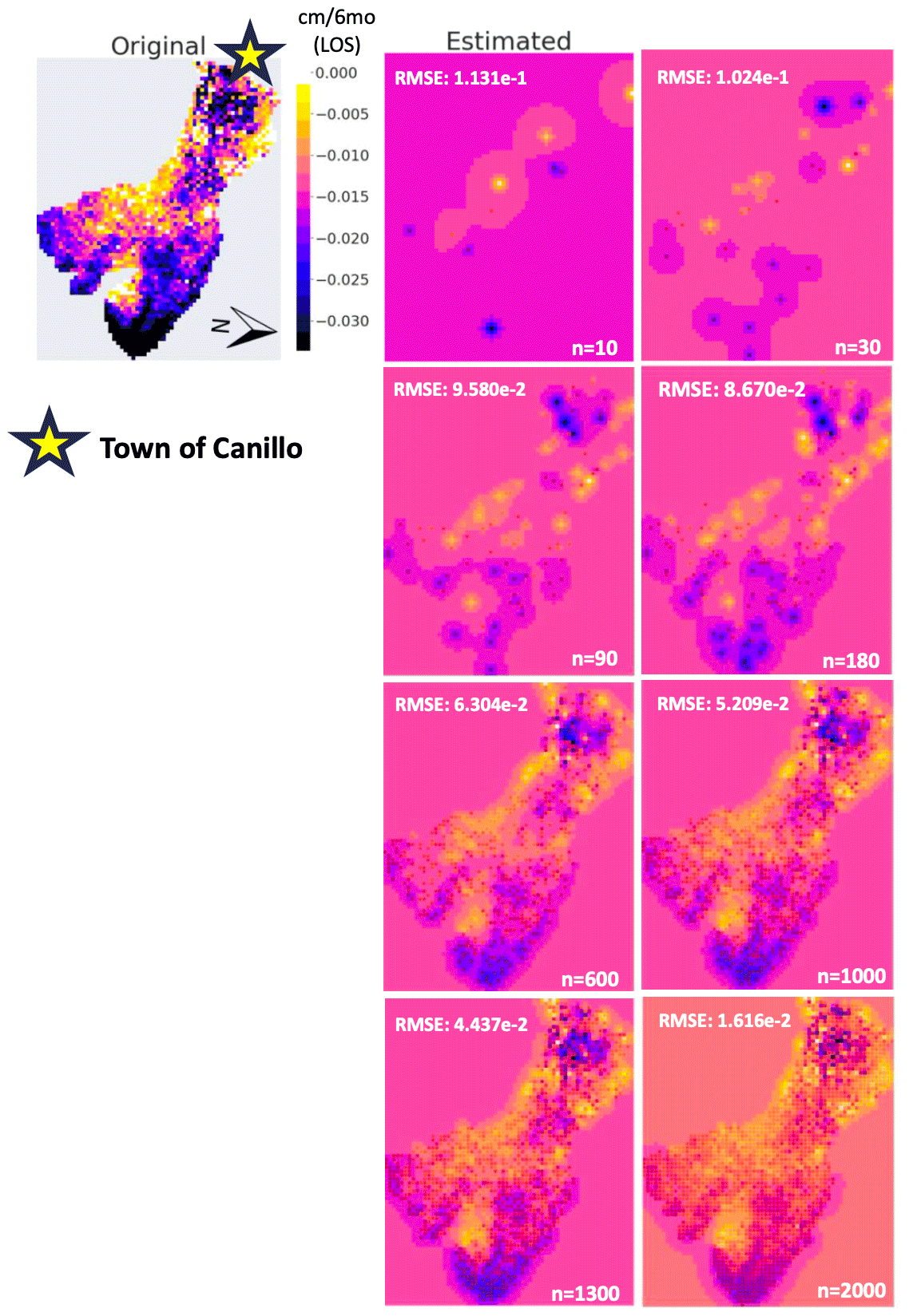
Figure 5 Results of ordinary kriging of various random samples (n=10–2000) via 1 iteration (as opposed to the 200 iterations of average velocity values; during the no-snow months of 2019 in the direction of the line of sight (LOS) in Fig. 3c), reflecting gaps in predictive capabilities on the surface of the landslide for further investigation. Normalized RMSE for each process of ordinary kriging indicating error for each sample size. The town of Canillo is marked with a star, and cardinal directions have been added for context.

4 Discussion

The application of interferometric synthetic-aperture radar (InSAR) for deep-seated landslide monitoring represents a significant advancement in geohazard assessment and management. The use of InSAR and its comparison to traditional in situ approaches for sub-surface ground motion serve as important next steps in assessing the viability of the remote sensing tool for large-scale deep-seated landslide monitoring. However, there are known limitations in this approach, including limited sub-surface in situ borehole readings to directly compare with InSAR. Additionally, as seen in Fig. 3, there is a trade-off between accuracy and precision when it comes to the use of InSAR for landslide detection versus monitoring. However, for considering the use of InSAR as a monitoring tool, this approach is limited in the assumption that the deep-seated landslide moves as a rigid block, as opposed to other deep-seated landslides that may move sequentially and not as uniformly. In the latter case, other sub-surface in situ measurements may be necessary to verify the movement of the landslide. There are, conversely, several advantages to the use of InSAR as a sub-surface monitoring tool, including its possibility of being linked with existing deep-seated landslide models (Veveakis et al., 2007; Seguí and Veveakis, 2022; Lau and Veveakis, 2024). The ability to correlate InSAR displacement readings with sub-surface ground motion, as addressed in this work, lends itself to be applied to well-developed models in which displacement from InSAR and in situ borehole readings can tune stability models for deep-seated landslides that use temperature in the landslide (frictional heating) as the primary driver for tertiary creep and catastrophic collapse of these large mass movements. With that in mind, there is an opportunity to apply InSAR as a forecasting tool. This opportunity, explored more in-depth in Lau and Veveakis (2024), has the potential to lead to a majority or, in some cases, completely remote approach to deep-seated landslide forecasting, utilizing InSAR and existing borehole data to develop and tune existing models for deep-seated landslide stability (Veveakis et al., 2007).

It is important to note, however, that the authors acknowledge that the best landslide-monitoring options often derive data from a variety of sources – remote sensing, in situ instrumentation, and narrative accounts. However, unlike ground-based methods, such as borehole instrumentation, which can be labor-intensive and expensive, InSAR provides comprehensive spatial coverage, with the capability of being applied to monitor remote or inaccessible regions. This is particularly beneficial for rural mountain communities who constantly face some degree of exposure to deep-seated landslides and who often reside in rugged terrains where installing and maintaining ground-based instruments can be challenging, costly, or financially inaccessible.

Of course, the results completed in this work could always be enhanced by the addition of more in situ monitoring options for the El Forn landslide to offer more direct comparison between InSAR and borehole displacement readings. Similarly, this work could be enhanced by more landslide case studies, perhaps with slopes facing other directions in order to better understand the sensitivity of in situ and InSAR data regarding the way the InSAR data were taken. Both of these possibilities for improvement are considered by the authors for future works.

5 Conclusions

In this paper, the use of InSAR for landslide monitoring was assessed for two key objectives: (1) correlation with in situ data to test the accuracy of InSAR in monitoring seasonal and off-seasonal sub-surface movement and (2) spacial interpolation across the landslide surface with various numbers of InSAR points to help us understand the use of InSAR for establishing areas on a scarp that need monitoring (i.e., further instrumentation), as well as understanding how many remote observations would allow us to minimize error in re-creating the scarp without using the full dataset. Correlation of the InSAR data with extensometer data in the S10 borehole on the El Forn scarp indicates that InSAR can be used to understand seasonal sub-surface ground motion.

The spatial interpolation, as well as the subsequent error assessment, conducted on the El Forn landslide using solely InSAR data helped determine the necessary number of observations to adequately monitor the general movement of the landslide. Based off of 200 iterations of random samples going through a process of ordinary kriging on the landslide, the outliers of the normalized root mean square error dropped significantly between 20 and 25 remote observations, as indicated in Fig. 4. Based off of Fig. 5, the most uncertainty, coupled with the most movement, though even an increased number of random samples are in the middle of the landslide, can be seen in the middle of the top left lobe, in the northeastern corner of the landslide. In future studies, we could look to perform regression kriging with 20–25 remote observations, focused solely on this region to understand how uncertainty propagates for this part of the landslide on a finer timescale. Overall, InSAR has many purposes when considering the monitoring of deep-seated landslides, with several options to build on our existing knowledge for studies to come.

Appendix A: Alaska Satellite Facility (ASF) InSAR workflow

The user-friendly interface of the Alaska Satellite Facility Vertex platform allows for easily specifying an InSAR pair. For this work, an interferometric-wide single-look complex (IW SLC) pair was selected, with SLC meaning that the SAR data have been compiled to an image but have not been multi-looked yet. Once the reference and dates of interest are selected, ASF begins multi-looking through various pairs of images. Note that for continuity purposes, the older SLC image is always used as the reference image.

In order to prepare a digital elevation model (DEM) file for subsequent geocoding and corrections, a topographic phase is subtracted from the interferogram by replicating an existing DEM to account for the actual topographic phase. In this case, Hyp3 takes the DEM from the publicly available 2021 release of the Copernicus GLO-30 DEM library. Removing this topographic phase from the interferogram, the deformation signal is all that remains (Hogenson et al., 2024).

Left with a stack of wrapped interferograms, phase unwrapping uses a minimum-cost flow (MCF) triangulation method to assign multiples of 2π to each pixel, which restricts the number of 2π jumps in phases to regions where they may occur. Note that thermal noise and interferometric decorrelation can result in 2π phase discontinuities, which are known as “residues” – these can be reduced via filtering. Filtering reduces phase noise and increases the accuracy of the interferometric phase by reducing the number of interferogram residues (Hogenson et al., 2024).

After filtering, a validity mask directs the unwrapping process by applying thresholds for coherence and amplitude (backscatter intensity) values for each image pair. For this work, this amplitude threshold is kept at 0.0, so coherence thresholds drive the masks. Coherence is estimated from a normalized interferogram, with a range from 0.0 to 1.0, with 1.0 being perfectly coherent. Once coherent thresholds are applied, unwrapping will proceed relative to a fixed pixel point. For this work, this point was selected as a rooftop in the town of Canillo at the foot of the landslide. This reference point is assigned an unwrapped phase value of 0 at this point, and every other pixel around it is then assigned a multiple of 2π with respect to that point.

Lastly, these pixels are reprojected from SAR slant range space into a map-projected ground range space and exported from the GAMMA internal format to the GeoTIFF format. These unwrapped interferograms are ready to be go through a time series inversion (Hogenson et al., 2024).