Rapid simulation of wave runup on morphologically diverse, reef-lined coasts with the BEWARE-2 (Broad-range Estimator of Wave Attack in Reef Environments) meta-process model

Low-lying, tropical, coral-reef-lined coastlines are becoming increasingly vulnerable to wave-driven flooding due to population growth, coral reef degradation, and sea-level rise. Early-warning systems (EWSs) are needed to enable coastal authorities to issue timely alerts and coordinate preparedness and evacuation measures for their coastal communities. At longer timescales, risk management and adaptation planning require robust assessments of future flooding hazard considering uncertainties. However, due to diversity in reef morphologies and complex reef hydrodynamics compared to sandy shorelines, there have been no robust analytical solutions for wave runup to allow for the development of large-scale coastal wave-driven flooding EWSs and risk assessment frameworks for reef-lined coasts. To address the need for fast, robust predictions of runup that account for the natural variability in coral reef morphologies, we constructed the BEWARE-2 (Broad-range Estimator of Wave Attack in Reef Environments) meta-process modeling system. We developed this meta-process model using a training dataset of hydrodynamics and wave runup computed by the XBeach Non-Hydrostatic process-based hydrodynamic model for 440 combinations of water level, wave height, and wave period with 195 representative reef profiles that encompass the natural diversity in real-world fringing coral reef systems. Through this innovation, BEWARE-2 can be applied in a larger range of coastal settings than meta-models that rely on a parametric description of the coral reef geometry. In the validation stage, the BEWARE-2 modeling system produced runup results that had a relative root mean square error of 13 % and relative bias of 5 % relative to runup simulated by XBeach Non-Hydrostatic for a large range of oceanographic forcing conditions and for diverse reef morphologies (root mean square error and bias 0.63 and 0.26 m, respectively, relative to mean simulated wave runup of 4.85 m). Incorporating parametric modifications in the modeling system to account for variations in reef roughness and beach slope allows for systematic errors (relative bias) in BEWARE-2 predictions to be reduced by a factor of 1.5–6.5 for relatively coarse or smooth reefs and mild or steep beach slopes. This prediction provided by the BEWARE-2 modeling system is faster by 4–5 orders of magnitude than the full, process-based hydrodynamic model and could therefore be integrated into large-scale EWSs for tropical, reef-lined coasts and used for large-scale flood risk assessments.

1 Introduction

Low-lying, tropical, coral-reef-lined coastlines are vulnerable to wave-driven overwash and flooding. These flooding events will become more frequent as sea level rises due to climate change (Vitousek et al., 2017; Vousdoukas et al., 2018), threatening infrastructure, ecosystems, and freshwater resources and infrastructure (Reynolds et al., 2015; Shimozono et al., 2015; Albert et al., 2016; Storlazzi et al., 2018). Globally, coral reefs protect more than 200 000 people living on the coast from flooding annually (Beck et al., 2018). These populations are denser, growing faster, and composed of more people from lower–middle income groups than the global average (Kumar and Taylor, 2015; Sing Wong et al., 2022). The combined increase in hazard probability and exposure leads to a higher likelihood of flood-related deaths (Chilunga et al., 2017). This increased risk necessitates the following: (1) better science and understanding of flood risk drivers in the tropics; (2) better, locally appropriate risk reduction and adaptation strategies to reduce coastal flooding and associated hazards (Hinkel et al., 2014); and (3) access to warning systems to increase preparedness and implement flood mitigation actions (Winter et al., 2020).

Short-term forecasts (typically up to 5–7 d) produced by early-warning systems (EWSs) allow authorities to issue timely warnings and coordinate preparation and evacuation measures, which ultimately reduce risk to lives and assets. Events such as Typhoon Haiyan (Roeber and Bricker, 2015) and widespread flooding of islands due to remotely generated swell in the western Pacific (Hoeke et al., 2013; Wadey et al., 2017; Ford et al., 2018; Wandres et al., 2020; Hoeke et al., 2021) highlight the need for warnings of impending coastal-flooding events. One-third of the world's population lives in areas that are not covered by EWSs, with particularly low EWS coverage in the least developed countries and small island developing states (WMO, 2022a). This issue has gained worldwide attention, and as a result the United Nations-endorsed Sendai Framework for Disaster Risk Reduction has called for improved access to early-warning systems and disaster risk assessments by 2030 (UNISDR, 2015).

EWSs have been implemented in sandy coastal environments (e.g., Doong et al., 2012; Coz et al., 2021; Stockdon et al., 2023), but reef-lined coasts demand different modeling approaches due to the complex bathymetry and wave dynamics characteristic of reef environments. Coral-reef-lined (fringing-reef) coasts are typically fronted by a shallow reef flat and a steeper fore reef farther offshore that dissipates open-ocean incoming wave energy through wave breaking and bottom friction (Lowe et al., 2005; Monismith et al., 2013). Wave breaking on the fore reef induces high radiation stress gradients, which results in significant wave-induced setup on the reef flat (Pomeroy et al., 2012; Beck et al., 2018). Some of the dissipated incident-band (sea–swell; >0.05 Hz) wave energy is transferred to the infragravity (IG) band (0.005–0.05 Hz) and very low-frequency (VLF) band waves (0.001–0.005 Hz) through breakpoint forcing (Symonds et al., 1982) on the steep fore reef (Péquignet et al., 2009; Pomeroy et al., 2012; Péquignet et al., 2014; Cheriton et al., 2016). Resonant amplification of IG and/or VLF waves can occur when their energy is concentrated at the natural frequency of the reef flat, which is most likely to occur on smooth reefs, with increasing water depth, high incident-band wave periods, and specific reef dimensions (Péquignet et al., 2009, 2014; Quataert et al., 2015; Gawehn et al., 2016; Pearson et al., 2017; Buckley et al., 2018). The complex interaction between tides, storm surge, the wave-induced setup, incident-band waves, IG waves, and VLF waves drives runup and subsequent flooding along reef-lined coasts.

Findings from sandy-beach investigations are not necessarily transferable to coral-reef-lined coasts. First, the bathymetric profiles of reef-lined coasts are starkly different from those of gently sloping beaches (Scott et al., 2020). Secondly, coral reefs can have much greater bed roughness, varying between the extremes of relatively smooth “pavement” reefs with little coral coverage and rough regimes with high coral coverage or/and bedrock rugosity (Quataert et al., 2015; Harris et al., 2018). Together, these severely limit the use of parametric models (e.g., Stockdon et al., 2006; Merrifield et al., 2014) in coral reef environments (see also Astorga-Moar and Baldock, 2023). Process-based models (e.g., Roelvink et al., 2009, 2018) have been adapted for coral-reef-lined coasts by modifying the typical wave action and/or non-linear shallow-water equations and parameterizing the hydrodynamic roughness in wave and friction factors (Van Dongeren et al., 2013; Quataert et al., 2015; Buckley et al., 2018; Lashley et al., 2018; de Ridder et al., 2021). However, although accurate, these models are very computationally expensive (e.g., Quataert et al., 2020) and therefore too slow for EWSs (Winter et al., 2020; WMO, 2022b). To capture the accuracy of process-based models in operationally feasible computational time frames, surrogate models, including meta-models (Pearson et al., 2017; Rueda et al., 2019; Liu et al., 2023), machine-learning models (Franklin and Torres-Freyermuth, 2022), and numerical model-informed empirical relations (Beetham and Kench, 2018), have been developed by running process-based models over a limited number of schematic coral reef bathymetries. However, as demonstrated by Scott et al. (2020), the natural variability in coral reef widths, depths, slopes, and rugosities (bathymetric variability) far exceeds the limited schematic bathymetries used in current surrogate models, limiting their accuracy and global applicability in EWSs.

To address this need for a fast, accurate EWS that accounts for the natural variability in coral reefs, we developed the Broad-range Estimator of Wave Attack in Reef Environments (BEWARE-2), a computationally efficient meta-process modeling system that estimates runup (wave-driven setup and swash) based on complex, process-based hydrodynamic model simulations. We developed BEWARE-2 using insights from the development of the BEWARE-1 meta-model (Pearson et al., 2017) and real-world coral reef profile clustering techniques of Scott et al. (2020) and trained the model to be suitable for application on a very large range of morphologically diverse, reef-lined coasts. Here we first detail the creation of a training database of representative, morphologically diverse reef profiles and the matching of real-world reef profiles to those representative profiles. Next, we document the application of the process-based hydrodynamic model XBeach Non-Hydrostatic (de Ridder et al., 2021) to the representative reef profiles over a broad range of oceanographic forcing conditions to generate hydrodynamic training data. We subsequently describe the application of BEWARE-2 to compute wave runup on a large variety of real-world coral reef profiles, describe the meta-process model validation, and quantify the predictive skill. Lastly, we discuss the meta-process model benefits, limitations, and application and next steps.

2 Methods

The BEWARE-2 meta-process modeling system is based on the non-hydrostatic version (de Ridder et al., 2021) of the open-source, process-based hydrodynamic model XBeach (Roelvink et al., 2009, 2018), henceforth referred to as XBNH, in order to estimate wave runup (wave-driven setup and swash) on reef-lined coasts. To do so, we developed a training dataset of hydrodynamics and wave runup computed by XBNH for varying hydrodynamic forcing conditions, similar to that of Pearson et al. (2017), for a set of morphologically diverse reef profiles, based on work by Scott et al. (2020), which is described in the following sections. Here we illustrate the different steps in the development of the meta-process modeling system.

2.1 Model training dataset

2.1.1 Representative reef profiles

A database of 195 representative, cross-reef profiles was created by combining parametric reef profiles from Pearson et al. (2017), real-world reef profiles from Scott et al. (2020), and additional wide-reef profiles identified in this study (Fig. 1). Coral reef profiles included in the BEWARE-1 model (Pearson et al., 2017) comprise 30 parametric representations of coral reef profile geometries found in the literature from 10 sites around the world (Quataert et al., 2015), with reef flat widths ranging from 0–500 m and fore reef slopes ranging from 0.1–0.5. The reef profiles of Scott et al. (2020) and the wide-reef profiles identified in this study (defined as profiles that reach a depth of 15 m at distances greater than 1.5 km offshore) were extracted from a dataset of 30 166 real-world coral reef profiles (Storlazzi et al., 2019), covering the coral-reef-lined coasts of the United States of America, US), including the states of Hawai'i and Florida; the territories of Guam, American Samoa (AmSamoa), and the US Virgin Islands (USVI); and the commonwealths of Puerto Rico (PuertoRico) and the Northern Mariana Islands. The dataset consists of transects with a 2 m cross-shore resolution spaced at 100 m intervals along the >3300 km of coastline. Of these transects, Scott et al. (2020) clustered 20 454 profiles with reef widths less than 1.5 km into 500 cluster groups and representative profiles, using data reduction techniques on morphology and hydrodynamics of the reef profiles. To allow for the application of BEWARE-2 in areas with wide reefs, such as barrier or extremely wide fringing reefs, additional profiles were derived in this study from the remaining 9712 reef transects with widths greater than 1.5 km. These profiles were clustered based on the submerged morphology in an identical fashion to that of Scott et al. (2020), leading to the identification of 20 representative wide-reef profiles.

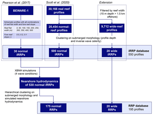
Figure 1 Flowchart outlining datasets and processes to develop both the 550 intermediate (iRRP) and final 195 representative reef profile (RRP) databases encompassing the 30 schematic reef profiles of Pearson et al. (2017), the 20 454 normal-reef profiles of Scott et al. (2020), and the 9712 wide-reef profiles excluded from the Scott et al. (2020) analysis but included here.

The 550 reef profiles described in the previous paragraph (i.e., 30 profiles following Pearson et al., 2017; 500 profiles following Scott et al., 2020; and 20 wide-reef profiles), henceforth termed the intermediate representative reef profiles (iRRPs), were subsequently reduced to set of 195 representative reef profiles (RRPs) for application in the BEWARE-2 training dataset. In doing this, 175 representative reef profiles (RRPs) were developed using the 30 iRRPs of Pearson et al. (2017) and 500 iRRPs of Scott et al. (2020), neither of which contain any very wide-coral-reef profiles (here termed the 530 normal iRRPs). In general, these 530 normal iRRPs have shapes characteristic of atoll and fringing-reef profiles. Following the methodology of Scott et al. (2020), the 530 normal iRRPs were reduced to 175 normal RRPs by means of hierarchical clustering based on two sets of features, namely the submerged morphology and nearshore hydrodynamics, which were assigned equal weighting. In line with Scott et al. (2020), the submerged morphology was expressed through both the profile depth and the inverse wave celerity, where the wave celerity (calculated from linear wave theory assuming a peak wave period T_p of 8 s) was included to give greater weight to shallower areas. The nearshore hydrodynamics features included the wave-driven setup, sea–swell and IG swash, and 2 % exceedance runup (R_2 %), computed using XBNH for four representative wave conditions. Similarly following Scott et al. (2020), each feature within each subset was transformed using a min–max linear scaler and equal weighting within the subset was assigned during clustering. During hierarchical clustering, iRRPs were progressively merged based on the smallest intergroup dissimilarity. After merging, an RRP was assigned for each group based on its proximity to the mean R_2 %. If there were more than one RRP with equal distance to the mean, the RRP that represented the larger number of profiles from the initial round of clustering was chosen. The number of cluster groups was set to 175 profiles based on the intra-cluster similarity of relevant hydrodynamic parameters, which resulted in a relative difference of less than 10 % for all four parameters. The 20 wide-reef iRRPs were directly mapped to wide-reef RRPs and added to the 175 normal RRPs, for a total dataset of 195 RRPs (Fig. 2).

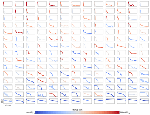
Figure 2 Overview of the morphology of the 195 representative reef profiles (RRPs), ordered from top left to bottom right by cross-shore distance to the 15 m depth contour (W_reef; see Sect. 3.2). The RRPs are color-coded according to the relative ranking of runup simulated by XBNH for a single representative wave condition ($H_{\mathrm{s},\mathrm{0}}=\mathrm{5}$ m, T_p=12 s), with blue indicating profiles with relatively lower wave runup and red indicating those with relatively higher wave runup.

2.1.2 XBNH process-based model description and setup

XBNH is a phase-resolving, non-hydrostatic model for the nearshore and coast. The model solves the non-linear shallow-water equations in a reduced two-vertical-layer system that includes a non-hydrostatic pressure term, allowing for application in shallow to intermediate water depth (kh⪅4, where $k=\frac{\mathrm{2}\mathit{\pi }}{L}$ is the wave number, h is the water depth, and L is the wavelength) with minimal dispersion errors (de Ridder et al., 2021). XBNH and the earlier one-layer non-hydrostatic version of XBeach (Smit et al., 2010) have previously been shown to reproduce laboratory and field measurements of wave transformation and runup on reef profiles well (e.g., Pearson et al., 2017; Lashley et al., 2018; Klaver et al., 2019; Masselink et al., 2019; Pomeroy and van Rooijen, 2019; Quataert et al., 2020; Masselink et al., 2020; de Ridder et al., 2021; Laigre et al., 2023).

XBNH models used for the training and validation of BEWARE-2 were set up in a one-dimensional (i.e., cross-shore transect) mode with spatially varying grid resolution and bed roughness. The grid resolution was optimized according to the local water depth and wave period, with a coarser grid being used at greater depths and for longer wave periods (64 points per local wavelength; minimum and maximum grid resolution of 0.25 and 5 m, respectively). The reef roughness was parameterized following Storlazzi et al. (2019), with a friction value (c_f) of 0.003 for the sandy beach and deep water. An increased reef friction (c_f=0.05) was implemented at all depths at which kh≤1 (i.e., depth less than 6.8–91.6 m, depending on the wave period given in Table 1) up to a minimum depth of 0.5 m. The offshore boundary location was established for each individual forcing condition, taking into account depth restrictions of $n=\frac{c_{\mathrm{g}}}{c}<\mathrm{0.75}$, where c_g is the group velocity and c is the wave celerity, to ensure correct infragravity wave boundary conditions, and kh<4 to allow for correct dispersion of the incident-band waves. Additionally, the ratio of maximum wave height to depth ($\frac{H_{\mathrm{s},\mathrm{0}}}{h}$, where H_s,0 is the deep-water significant wave height) was set to 0.25 to prevent wave breaking at the boundary. Resulting offshore water depths vary between 30 and 58 m. Where necessary, the profiles were extended from the original RRP depth of 30 m to the offshore water depth required for the forcing conditions using an artificial slope of $\mathrm{1}/\mathrm{10}$. To enable computations for the full range of hydrodynamic conditions without runup exceeding the profiles' beach crest, an artificial semi-infinite beach was created extending from 0–30 m a.m.s.l. (above mean sea level) with a slope of $\mathrm{1}/\mathrm{10}$. Key model parameters were adopted from Quataert et al. (2020), with model wave breaker parameters maxbrsteep and reformsteep, which control the onset and cessation of wave breaking in the non-hydrostatic model, set to 0.6 and 0.3, respectively, and other model parameters set to their default value.

2.1.3 XBNH simulations and output

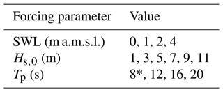
The XBNH models were developed to simulate wave runup on each RRP for 440 combinations of the offshore still-water level (SWL; 0–4 m a.m.s.l.), H_s,0 (1–11 m), and T_p (6–22 s) (see Table 1 for values applied in this study). To avoid the use of unrealistic wave conditions, H_s,0–T_p combinations with a deep-water wave steepness ($s_{\mathrm{0}}=\frac{\mathrm{2}\mathit{\pi }{H}_{\mathrm{s},\mathrm{0}}}{g{T}_{\mathrm{p}}^{\mathrm{2}}}$, where g is the gravitational constant) greater than 0.075 were removed. Consequently, no H_s,0 values greater than 4 and 7 m were applied in combination with T_p values of 6 and 8 s, respectively. Time series of random realizations of incident-band and wave-group-bound IG waves were generated internally by the model (see Roelvink et al., 2009) for each SWL–H_s,0–T_p forcing combination assuming normally incident offshore waves and a JONSWAP spectral shape (peak enhancement factor γ=3.3; Hasselmann et al., 1973) and an approximate directional spread of 24° (s=10 in the cos^2s directional-spread model). Simulations of all RRPs used the same time series of random incident waves per SWL–H_s,0–T_p combination to allow for direct comparison of hydrodynamics between RRPs. All simulations were run for a period of 800 T_p (i.e., approximately 800 waves), of which the period of the first 300 T_p was used as model spinup and model output from the final 500 T_p was used for runup analysis.

Table 1 Overview of hydrodynamic forcing conditions used in the training dataset. ^* Note: wave height combinations for T_p≤8 s are constrained by maximum deep-water wave steepness (s₀≤0.075).

The XBNH models were set to output the time series of the horizontal and vertical position of the simulated waterline at a temporal resolution of $\frac{T_{\mathrm{p}}}{\mathrm{20}}$ (i.e., 0.3–1.1 s). The value of R_2 % was derived from the vertical waterline position time series following Stockdon et al. (2006). Output time series for each simulation were split into five time frames of 100 T_p (i.e., approximately 100 waves) to provide five estimates of the empirical R_2 % value per simulation. In a limited number of simulations, waterline position time series were split into four or three (6.2 % and 2.3 % of simulations, respectively) time frames to ensure there were sufficient runup maxima in each period to determine the empirical R_2 % value. These runup data are provided in the BEWARE-2 database (McCall et al., 2024).

In addition to the time series of the simulated waterline, XBNH output time series of water levels, depth-averaged velocity, and horizontal discharge were stored for the offshore boundary of the model, 8 locations across the reef profile, and 15 positions on the beach face at a temporal resolution of $\frac{T_{\mathrm{p}}}{\mathrm{20}}$, which may in the future be used to estimate nearshore wave heights and overtopping rates. These data are not discussed further in this paper.

2.2 Meta-process model description

Application of BEWARE-2 to estimate wave runup for a given real-world “target” reef profile and real-world target oceanic boundary conditions follows a three-step process (Fig. 3). These three steps are discussed in the following sections.

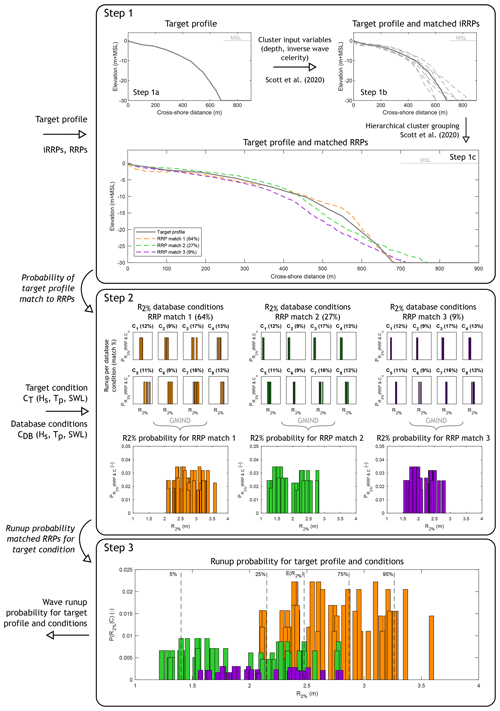
Figure 3 Schematic displaying the steps in the application of BEWARE-2 to compute a runup, in this case using three representative reef profiles (RRPs) matched to the real-world target bathymetric profile. Step 1: match the target profile to RRPs and their relative match probability. Step 2: for each RRP, extract runup values associated with the oceanographic forcing conditions in the BEWARE-2 database, bounding the target oceanographic forcing conditions and their probabilities relative to the target forcing oceanographic conditions using the geometric mean inverse normalized distance (GMIND). Step 3: combine the database runup probabilities associated with each RRP and their relative weighting to the RRP to compute an expected and/or exceedance probability runup.

2.2.1 Step 1: matching the target bathymetric profile to representative reef profiles (RRPs)

Probabilistic matching of a real-world target bathymetric profile to the representative reef profiles (RRPs) involves three steps (Fig. 3, top panel). First, the cluster input variables (i.e., depth and inverse wave celerity) are generated (Step 1a). Second, the target profile is probabilistically matched to the 550 iRRPs (Step 1b). Finally, the result of the matching to the 550 iRRPs is transformed to the 195 RRPs through the hierarchical tree (Step 1c).

The cluster input variables for the probabilistic profile matching in Step 1a are computed following the same procedure for the submerged morphology clustering as Scott et al. (2020) (see Sect. 2.1.1). For both the target profile and the 550 iRRPs, the clustering variables are weighted by 50 % for the profile depths and 50 % for the inverse wave celerities.

The distance between the target profile and the 550 iRRPs in Step 1b is calculated using the city block distance metric (e.g., Melter, 1987). The softmax function (Bridle, 1990) subsequently transforms the vector of real values, in this case the normalized cluster parameter distances, and a stiffness parameter (β_softmax) into probabilities of the target profile matching to the iRRPs (p_P,iRRP):

$$\begin{array}{}\text{(1)}& p_{\mathrm{P},\mathrm{iRRP},i}={\displaystyle \frac{e^{-{\mathit{\beta }}_{\mathrm{softmax}}{d}_i}}{\sum _{j=\mathrm{1}}^{N_{\mathrm{iRRP}}}{e}^{-{\mathit{\beta }}_{\mathrm{softmax}}{d}_j}}},\end{array}$$

where $p_{\mathrm{P},\mathrm{iRRP},i}$ is the matching probability of the target profile to iRRP i, d_i is the distance between the target profile and iRRP i, d_j is the distance between the target profile and iRRP j, and N_iRRP=550 is the total number of iRRPs.

The stiffness parameter β_softmax can be seen as a concentration parameter controlling entropy. Larger values of β_softmax result in narrower distributions, corresponding to higher probabilities associated with small absolute-distance metrics between the target profile and the iRRPs (and similarly, low probabilities for large absolute-distance metrics). The value of β_softmax is initially set to 1200, following Scott et al. (2020). A varying β_softmax can improve matching outcomes if entropy is too small or large; i.e., many or few iRRPs profiles match the target profile (Bakker et al., 2022). Thus a varying stiffness criterion is established on the distance metric entropy and ultimately converted to profile-matching threshold numbers. Specifically, if the number of iRRPs that a target profile matches to is less than four, β_softmax is stepwise relaxed until 4 iRRPs are matched. Conversely, if the target profile matches more than 10 iRRPs, β_softmax is incrementally tightened, with the additional benefit of improving computational efficiency during interpolation.

Finally, in Step 1c, the matched iRRPs are linked to RRPs following the hierarchical clustering tree (i.e., linking 530 iRRPs to 175 RRPs) in the case of regular reef profiles, and in the case of wide-reef profiles, the tree branch is a direct iRRP–RRP matching (see Fig. 1). Note that due to hierarchical clustering of iRRPs to RRPs, the minimum number of matched RRPs may be less than four. Where multiple matched iRRPs link to the same RRP through hierarchical clustering, the final probability of profile matching between the target profile and the RRP (p_P,RRP) is computed by summing the match probabilities of all linked iRRPs.

2.2.2 Step 2: computing runup estimates for matched RRPs based on target oceanic conditions

Wave runup estimates for the target oceanic forcing condition C_T (H_s,0, T_p, SWL) are generated for each matched RRP (Fig. 3, center panel). For each matched RRP, all BEWARE-2 R_2 % values associated with the oceanic conditions bounding (higher and lower) the target oceanic condition are identified in the BEWARE-2 database, resulting in 2³=8 bounding oceanic conditions C_DB (all combinations of the nearest greater and lesser database values of H_s,0, T_p, and SWL relative to the target oceanic condition). For example, if the target oceanographic conditions are values of $H_{\mathrm{s},\mathrm{0}}=\mathrm{4.2}$ m, T_p=13.7 s, and SWL=1.4 m, R_2 % for all combinations of $H_{\mathrm{s},\mathrm{0}}=[\mathrm{4},\mathrm{5}]$ m, $T_{\mathrm{p}}=[\mathrm{12},\mathrm{14}]$ s, and $\mathrm{SWL}=[\mathrm{1},\mathrm{2}]$ m, conditions would be identified in the BEWARE-2 database. Each BEWARE-2 R_2 % value is then assigned a weighting factor proportional to the geometric mean inverse normalized distance (GMIND) between the target oceanographic condition and that in the BEWARE-2 database:

$$\begin{array}{}\text{(2)}& \mathrm{GMIND}\left(n\right)={\left(\prod _{j=\mathrm{1}}^J\mathrm{1}-\left|{\displaystyle \frac{X_{j,n}-Y_j}{\mathrm{\Delta }{X}_j}}\right|\right)}^{\frac{\mathrm{1}}{J}},\end{array}$$

where n=1, …, 8 is the index of the eight (2^J) nearest oceanic conditions in the database, J=3 is the number of oceanic forcing variables (i.e., H_s,0, T_p, and SWL), X_j,n is the value of variable j in the database oceanic condition C_DB(n), Y_j is the target oceanic condition for variable j, and ΔX_j is the spacing of variable j in the BEWARE-2 oceanic condition dataset.

The probability weighting ($p_{C_{\mathrm{DB}}|C_{\mathrm{T}}}\left(n\right)$) between the target condition C_T and each of the eight nearest oceanic conditions in the database (C_DB(n)) is found by normalizing GMIND(n) for each C_DB condition by the sum of GMIND for all eight (2^J) C_DB values:

$$\begin{array}{}\text{(3)}& p_{p_{C_{\mathrm{DB}}|C_{\mathrm{T}}}\left(n\right)}={\displaystyle \frac{\mathrm{GMIND}\left(n\right)}{\sum _{m=\mathrm{1}}^{{\mathrm{2}}^J}\mathrm{GMIND}\left(m\right)}}.\end{array}$$

The weighted nearest-neighbor-type approach described above to assign probability weights to database conditions is different from the Bayesian-based interpolation applied in the BEWARE-1 meta-model. However, in Sect. 2.4 we will show that the relatively simple and explainable machine-learning approach applied in BEWARE-2 is easily sufficiently accurate for practical application.

2.2.3 Step 3: computing runup estimates for the target profile and target oceanic conditions

To compute the overall expected and/or exceedance probability R_2 % for a target profile and target oceanic forcing conditions, the R_2 % probabilities of Step 2 ($p_{C_{\mathrm{DB}}|C_{\mathrm{T}}}\left(n\right)$) are multiplied by the probabilities of a profile match of Step 1 (p_P,RRP; Fig. 3, bottom panel). Based on the weighted R_2 % values, the expected value and exceedance probability value for R_2 % can be established through an empirical cumulative density function.

2.3 Accounting for variations in reef roughness and beach slope

The BEWARE-2 training dataset is composed of the results of XBNH simulations of 195 RRPs and under varying conditions of SWL, H_s,0, and T_p; geometric and hydrodynamic parameters that were found by Pearson et al. (2017) to contribute most to variations in wave runup. However, the training dataset only contains simulations that have constant values for the hydrodynamic roughness of the reef ($c_{\mathrm{f},\mathrm{ref}}=\mathrm{0.05}$) and slope of the subaerial beach (${\mathit{\beta }}_{\mathrm{b},\mathrm{ref}}=\mathrm{0.10}$), which were found by Pearson et al. (2017) to contribute least to variations in wave runup. Despite their lesser significance for wave runup on coral-reef-lined coasts, inclusion of coral reef roughness and beach slope in BEWARE-2 may be relevant to first-order assessments of the effect of reef health (expressed through c_f) and (seasonal) morphological change of the beach (expressed through β_b) on wave runup. Although it would technically be feasible to include variations in c_f and β_b in the training dataset, this would require an undesirable increase in the number of XBNH simulations and computation time (e.g., a 9-fold increase in computational expense for a minimum of three permutations per parameter or a 25-fold increase for five permutations per parameter). Therefore, an alternative approach is taken to estimate RRP-specific contributions of reef roughness and beach slope to wave runup.

The methodologies derived to estimate the effect of reef roughness and beach slope variations on wave runup are described in full in Appendix A. In summary, the methodologies utilize a limited dataset of XBNH simulations of 31 reef profiles with varying hydrodynamic parameters and varying values of c_f and β_b (Appendix A1) to calibrate physics-based relations for a relative increase or decrease in wave runup using known morphological and hydrodynamic parameters. The resulting relations used to estimate relative changes in wave runup due to variations in reef roughness and beach slope are described in Sect. 2.3.1 and 2.3.2, respectively. A full description of the derivation and calibration of these relations is given in Appendix A2 and A3, respectively.

2.3.1 Reef roughness

Increased or decreased wave runup ($R_{\mathrm{2}\mathit{\%}}^{\mathrm{m},\mathrm{r}}$; Eq. 4) relative to the standard BEWARE-2 runup estimate (R_2 %) due to decreased or increased reef roughness, respectively, is approximated by estimating the relative change in wave height reaching the shore. To do so, a simple wave energy balance model using linear wave theory, the deep-water wave conditions, and reef geometry but excluding bed friction effects, described in Appendix A2, is used to estimate the cross-shore varying near-bed wave orbital (u_orb) and wave group (c_g) velocity. This velocity is integrated over the cross-shore extent of the model domain with a hydrodynamic roughness value of c_f=0.05 ($L_{c_{\mathrm{f}}}$), i.e., the cross-shore extent of the coral reef, to provide a first-order estimate of potential energy loss on the reef due to bed friction (Γ_reef; Eq. 7). The potential energy loss estimate is subsequently scaled by the difference in roughness of the reef (c_f) relative to the reference reef roughness included in the training dataset ($c_{\mathrm{f},\mathrm{ref}}=\mathrm{0.05}$; Eq. 6), H_s,0, the gravitational constant (g), and a calibration coefficient (α_r) to compute a wave runup modification factor (F_r; Eq. 5).

$$\begin{array}{}\text{(4)}& {\displaystyle }& {\displaystyle }{R}_{\mathrm{2}\mathit{\%}}^{\mathrm{m},\mathrm{r}}=R_{\mathrm{2}\mathit{\%}}{F}_{\mathrm{r}}\text{(5)}& {\displaystyle }& {\displaystyle }{F}_{\mathrm{r}}=\max \left(\mathrm{1}+{\mathit{\alpha }}_{\mathrm{r}}{\displaystyle \frac{{\mathit{\gamma }}_{\mathrm{r}}}{\sqrt{g}{H}_{\mathrm{s},\mathrm{0}}}}{\mathrm{\Gamma }}_{\mathrm{reef}},\mathrm{0}\right)\text{(6)}& {\displaystyle }& {\displaystyle }{\mathit{\gamma }}_{\mathrm{r}}=\sqrt{|{\displaystyle \frac{c_{\mathrm{f}}}{c_{\mathrm{f},\mathrm{ref}}}}-\mathrm{1}|}\text{(7)}& {\displaystyle }& {\displaystyle }{\mathrm{\Gamma }}_{\mathrm{reef}}=\sqrt{\underset{L_{c_{\mathrm{f}}}}{\int }{\displaystyle \frac{u_{\mathrm{orb}}^{\mathrm{3}}\left(x\right)}{c_{\mathrm{g}}\left(x\right)}}\mathrm{d}x}\end{array}$$

A full description of the derivation of Eqs. (4)–(7) and the calibration of α_r is given in Appendix A2. In summary, separate values of α_r were calibrated for reef profiles with relatively low roughness and relatively high roughness, resulting in ${\mathit{\alpha }}_{\mathrm{r},\mathrm{smooth}}=\mathrm{1.16}$ for a relatively smooth reef (c_f=0.01) and ${\mathit{\alpha }}_{\mathrm{r},\mathrm{rough}}=-\mathrm{0.65}$ for a relatively rough reef (c_f=0.10). Although the application of these calibrated values is intended to illustrate likely upper and lower limits of wave runup for natural reefs in poor or good health, interpolation between the calibrated values for specific intermediate values of c_f likely exceeds the accuracy of the methodology and is therefore not recommended.

2.3.2 Beach slope

In an approach similar to that for variations in reef roughness, wave runup on steeper or milder beach slopes than those included in the BEWARE-2 training dataset ($R_{\mathrm{2}\mathit{\%}}^{\mathrm{m},\mathrm{b}}$) can be estimated by applying Eq. (8). In doing this, a linear wave runup correction factor (F_b; Eq. 9), inspired by the work of Stockdon et al. (2006), is computed using information in the BEWARE-2 training dataset on the hydrodynamic components of wave runup. Here, η_surf, η_swash, S_IG, and S_inc are the surf-zone setup, setup inside the swash zone, infragravity-band swash, and incident-band swash components of wave runup, respectively, and ${\mathit{\eta }}_{\mathrm{surf}}+{\mathit{\eta }}_{\mathrm{swash}}={\mathit{\eta }}_{\mathrm{wl}}$ represents the combined time-averaged setup at the shoreline. Following Stockdon et al. (2006), variations in beach slope (β_b) are assumed to affect S_inc but not S_IG. Furthermore, it is assumed that the beach slope affects the water level setup at the shoreline (Stockdon et al., 2006), but that this can be separated into a surf-zone component, which is assumed to depend only on the reef and shoreface morphology, and a beach-slope-dependent swash-zone component. The contribution of beach slope variations to S_inc and η_swash is set through the calibration coefficient α_b.

$$\begin{array}{}\text{(8)}& {\displaystyle }& {\displaystyle }{R}_{\mathrm{2}\mathit{\%}}^{\mathrm{m},\mathrm{b}}=R_{\mathrm{2}\mathit{\%}}{F}_{\mathrm{b}}\text{(9)}& {\displaystyle }& {\displaystyle }{F}_{\mathrm{b}}={\displaystyle \frac{\stackrel{\mathrm{‾}}{{\mathit{\eta }}_{\mathrm{surf}}+{\mathit{\alpha }}_{\mathrm{b}}\stackrel{\mathrm{‾}}{{\mathit{\eta }}_{\mathrm{swash}}}+\frac{\sqrt{S_{\mathrm{IG}}^{\mathrm{2}}+{\left({\mathit{\alpha }}_{\mathrm{b}}{S}_{\mathrm{inc}}\right)}^{\mathrm{2}}}}{\mathrm{2}}}}{\stackrel{\mathrm{‾}}{{\mathit{\eta }}_{\mathrm{surf}}}+\stackrel{\mathrm{‾}}{{\mathit{\eta }}_{\mathrm{swash}}}+\frac{\sqrt{S_{\mathrm{IG}}^{\mathrm{2}}+S_{\mathrm{inc}}^{\mathrm{2}}}}{\mathrm{2}}}}\end{array}$$

Although it might be expected that α_b would scale linearly with changes in beach slope, comparison to the calibration data (Appendix A3) shows that linear scaling does not improve the predictive skill of the model. Instead, a heuristic non-linear relation is found between α_b and the change in beach slope (Eq. 10):

$$\begin{array}{}\text{(10)}& {\mathit{\alpha }}_{\mathrm{b}}={\left({\displaystyle \frac{{\mathit{\beta }}_{\mathrm{b}}}{{\mathit{\beta }}_{\mathrm{b},\mathrm{ref}}}}\right)}^{{\mathit{\kappa }}_{\mathrm{b}}},\end{array}$$

where ${\mathit{\beta }}_{\mathrm{b},\mathrm{ref}}=\mathrm{0.10}$ is the reference beach slope included in the BEWARE-2 training dataset. The value of ${\mathit{\kappa }}_{\mathrm{b}}=\frac{\mathrm{1}}{e}$ was calibrated by minimizing the relative bias (RB) of the predicted wave runup in the calibration dataset, as described in Appendix A3. As the non-linear nature of Eq. (10) is not fully understood, extrapolation to beach slopes outside the range of the calibration simulations (i.e., β_b=0.05–0.20) is not recommended.

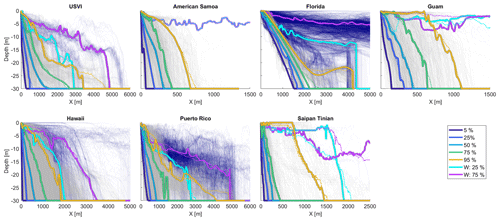
Figure 4 Observed real-world normal (gray) and wide (dark blue) cross-shore reef profiles for each of the seven geographic regions included in the dataset of Storlazzi et al. (2019), indicating the natural variability in reef morphologies. Colored dashed lines indicate the cross-shore varying statistical 5 %, 25 %, 50 %, 75 %, and 95 % depth exceedance values. Colored solid lines indicate the real-world profiles most similar to each depth exceedance, which were used for model validation. For the wide reefs, only the 25 % and 75 % depth exceedance profiles were extracted for model validation.

2.4 Meta-process model validation

2.4.1 Validation dataset

The ability of the BEWARE-2 meta-process model to predict R_2 % of morphologically diverse reefs and under varying hydrodynamic forcing conditions is quantified using a validation dataset of 24 000 process-based, XBNH model simulations that are separate from the dataset of simulations used to train the meta-process model. To develop the validation dataset, five normal and one to two wide, real cross-shore profiles were selected from each of the seven geographic regions (Guam, Saipan–Tinian (SaipanTinian), American Samoa, Hawai'i, Florida, Puerto Rico, and the US Virgin Islands) included in the dataset of Storlazzi et al. (2019), for a total of 35 normal and 13 wide-reef profiles. Normal-reef profiles representative of the morphological diversity in every geographic region in the dataset of Storlazzi et al. (2019) (i.e., 20 454 profiles in total; see Sect. 2.1.1) were selected by first statistically determining the 5 %, 25 %, 50 %, 75 %, and 95 % depth exceedance values at every cross-shore position (i.e., the depth exceeded by a given percentage of the observed profiles at every cross-shore position; Fig. 4, dashed lines). Subsequently, the observed, real-world profiles most similar to the cross-shore varying 5 %, 25 %, 50 %, 75 %, and 95 % depth exceedance values (Fig. 4, solid lines) were selected for the validation dataset. Wide-reef profiles were similarly selected for each geographic region from the dataset of wide-coral-reef profiles of Storlazzi et al. (2019) (i.e., 9712 profiles in total; see Sect. 2.1.1). For all geographic regions except American Samoa, the nearest observed profiles to the 25 % and 75 % depth exceedance of wide profiles were selected for the validation dataset. In American Samoa, the only wide profile included in the database of Storlazzi et al. (2019) was selected. None of the 48 (35 normal- and 13 wide-reef) validation profiles were identical to the RRPs included in the training dataset.

The XBNH models were set up for all 48 validation profiles using the same model settings and procedure as described in Sect. 2.1.2. Each validation profile was forced with the same set of 100 combinations of SWL, H_s,0, and T_p, where values of SWL, H_s,0, and T_p were randomly sampled between the minimum and maximum values included in the training dataset (Table 1) following independent uniform probability distributions. In a fashion similar to the training dataset, no combinations of H_s,0 and T_p with a deep-water wave steepness greater than 0.075 were included in the validation dataset. Parameters of wave spectral frequency and directional spread were kept the same as in the training dataset (Sect. 2.1.3).

Parameter values for the reef roughness and beach slope are initially kept the same as in the training dataset. Thus, the validation dataset contains 4800 simulations (48 profiles, 100 oceanic forcing conditions) with the trained values for reef roughness ($c_{\mathrm{f},\mathrm{ref}}=\mathrm{0.05}$) and beach slope (${\mathit{\beta }}_{\mathrm{b},\mathrm{ref}}=\mathrm{0.10}$). However, to validate the R_2 % modification relations for reef roughness and beach slope described in Sect. 2.3.1 and 2.3.2, additional XBNH simulations were carried out for each combination of the validation reef profiles and oceanic forcing conditions in which either the reef roughness (c_f=0.01 or c_f=0.10) or the beach slope (β_b=0.05 or β_b=0.20) was increased or decreased relative to c_f,ref or β_b,ref, respectively. These reef roughness and beach slope variations compose 19 200 simulations (four variations of roughness and slope for all 4800 combinations of reef profiles and oceanic forcing conditions).

The combined 24 000 XBNH validation simulations were run for a period of 800 T_p (of which the first 300 T_p was used as a spinup), as was the case for the training dataset. R_2 % simulated in the XBNH validation models was derived as described in Sect. 2.1.3. BEWARE-2 R_2 % predictions were calculated using the profile-matching and R_2 % extraction procedures described in Sect. 2.2. Where relevant, BEWARE-2 R_2 % predictions were modified for the reef roughness and beach slope following the procedures described in Sect. 2.3.

2.4.2 Model skill quantification

The skill of the BEWARE-2 meta-process model in reproducing R_2 % simulated by XBNH for the validation dataset was quantified by five measures of accuracy: the root mean square error (RMSE; Eq. 11), the model bias (bias, Eq. 12), the scatter index (SI) (or non-dimensional RMSE; Eq. 13), the relative (or non-dimensional) bias (RB; Eq. 14), and the coefficient of determination (R²; Eq. 15).

$$\begin{array}{}\text{(11)}& {\displaystyle }& {\displaystyle }\mathrm{RMSE}=\sqrt{\stackrel{\mathrm{‾}}{(X^{\prime }-X{)}^{\mathrm{2}}}}\text{(12)}& {\displaystyle }& {\displaystyle }\mathrm{Bias}=\stackrel{\mathrm{‾}}{(X^{\prime }-X)}\text{(13)}& {\displaystyle }& {\displaystyle }\mathrm{SI}={\displaystyle \frac{\mathrm{RMSE}}{\stackrel{\mathrm{‾}}{X}}}\text{(14)}& {\displaystyle }& {\displaystyle }\mathrm{RB}={\displaystyle \frac{\mathrm{bias}}{\stackrel{\mathrm{‾}}{X}}}\text{(15)}& {\displaystyle }& {\displaystyle }{R}^{\mathrm{2}}=\mathrm{1}-{\displaystyle \frac{\stackrel{\mathrm{‾}}{(X^{\prime }-X{)}^{\mathrm{2}}}}{\stackrel{\mathrm{‾}}{(X-\stackrel{\mathrm{‾}}{X}{)}^{\mathrm{2}}}}}\end{array}$$

In Eqs. (11)–(15), X represents the R_2 % level simulated by XBNH, X^′ represents the R_2 % level predicted by BEWARE-2, and an overbar represents the arithmetic mean.

3 Results

3.1 Profile matching

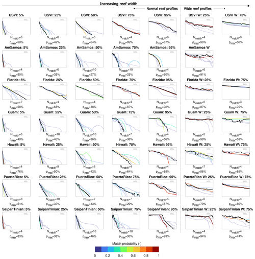
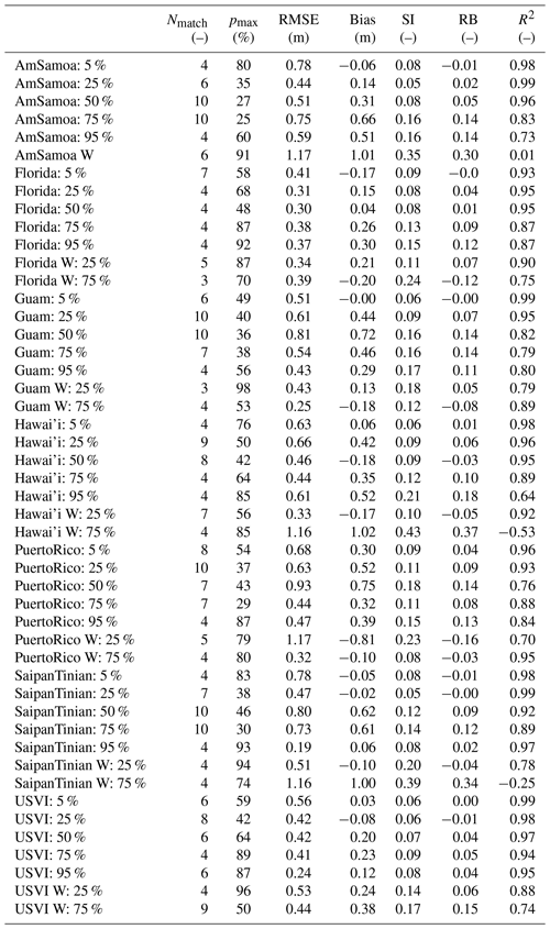
The first step in the BEWARE-2 meta-process model is the probabilistic matching of the target profile to the database RRPs (see Fig. 3). Here, the validation reef profiles (solid colored lines in Fig. 4) were probabilistically matched with between 3 and 10 RRP profiles (N_match; median value of 5.5) using the methodology described in Sect. 2.2 (Fig. 5 and Table A2). In the majority of cases (32 out of 48), the target profile matching included one RRP with at least a 50 % probability of matching ($p_{\mathrm{P},\mathrm{RRP}}>\mathrm{0.5}$). In six cases (US Virgin Islands W 25 %, American Samoa W, Florida 95 %, Guam W 25 %, Saipan–Tinian 95 %, and Saipan–Tinian W 25 %) the target profile was matched very strongly ($p_{\mathrm{P},\mathrm{RRP}}>\mathrm{0.9}$) to a single RRP. Three cases (American Samoa 50 %, American Samoa 75 %, and Puerto Rico 75 %) had a poor probability of matching ($p_{\mathrm{P},\mathrm{RRP}}<\mathrm{0.3}$) for all matched RRPs, with the poorest probability of matching occurring for the American Samoa 75 % profile (maximum match probability of 25 %).

Figure 5 Probabilistic matching of the 48 validation profiles (thick black lines) to RRPs (colored lines). Probability of matching to each RRP is indicated by the color of the RRP. The number of matched RRPs (N_match) and maximum matching probability (p_max) is given below each panel.

3.2 Runup prediction

Values of R_2 % vary substantially between validation profiles (Fig. 6), with maximum R_2 % on the narrower-reef profiles (e.g., 5 % profiles of the US Virgin Islands, American Samoa, Hawai'i, and Saipan–Tinian) being approximately 4–5 times greater than on the wide-reef profiles. BEWARE-2 R_2 % predictions (expected value) compare very well with simulated R_2 % results of XBNH for almost all 35 normal-reef validation profiles and almost half of the 13 wide-reef validation profiles.

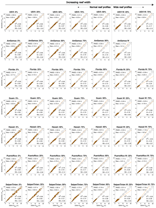
Figure 6 Values of R_2 % simulated by XBNH (horizontal axis) and the expected-value prediction of BEWARE-2 (vertical axis) for all oceanic forcing conditions and each validation profile. Included are the 1:1 relation (solid black line), 10 % upper and lower deviation from 1:1 (dashed black lines), and linear regression through the data (solid orange line).

For the 35 normal-reef validation profiles, RMSE and bias vary between 0.19–0.93 and −0.18–0.75 m, respectively, whereas SI and RB vary between 0.05–0.21 and −0.04–0.18, respectively (see also Table A2). The coefficient of determination is high (R²≧0.80) for 31 out of 35 validation profiles, with a minimum of R²=0.64 (Hawai'i 95 %). The two normal validation profiles that matched very strongly to a single RRP have similar accuracy measures to the overall dataset (Florida 95 %: SI = 0.15, RB = 0.12; Saipan–Tinian 95 %: SI = 0.08, RB = 0.02). Similarly, the three cases that had poor probability of matching do not suffer from a substantial reduction in accuracy (American Samoa 50 %: SI = 0.08, RB = 0.05; American Samoa 75 %: SI = 0.16, RB = 0.14; Puerto Rico 75 %: SI = 0.11, RB = 0.08). Overall, there is no significant correlation (Pearson correlation coefficient of 0.01; p value of 0.94) between the accuracy of BEWARE-2 (in this case simplified to only SI, but similar results are found for RB) and the highest probability of matching (p_P,RRP) to an RRP. This suggests that the maximum matching probability to RRPs is not a key factor determining model skill and that the accuracy of the BEWARE-2 meta-process model will remain broadly similar for all normal-reef profiles, independent of their morphological similarity to the RRPs.

For the 13 wide-reef validation profiles, RMSE and bias vary between 0.25–1.17 and $-\mathrm{0.81}-$–0.02 m, respectively, whereas SI and RB vary between 0.08–0.43 and −0.16–0.37, respectively. Only 5 of the 13 wide-reef validation profiles have a high coefficient of determination (R²≧0.80). It is therefore apparent that the accuracy of the BEWARE-2 meta-process model is substantially lower on wide-reef profiles (e.g., barrier or extremely wide fringing reefs) than on normal-reef profiles. Again for the wide-reef validation profiles, there is no clear correlation between the accuracy of BEWARE-2 and a high probability matching to RRPs (Pearson correlation coefficient of 0.22; p value of 0.47), exemplified by the relatively low accuracy for American Samoa W (one of six cases to match very strongly to one RRP; SI = 0.35, RB = 0.30) and the relatively high accuracy of Hawai'i W 25 % (matched to seven RRPs maximally with $p_{\mathrm{P},\mathrm{RRP}}=\mathrm{0.56}$; SI = 0.10, RB = −0.05).

Model skill metrics for the entire validation dataset (Fig. 7, left panel) are generally similar to those of the individual validation profiles, with an RMSE and bias of 0.63 and 0.26 m, respectively, and SI and RB of 0.13 and 0.05, respectively. Model accuracy is generally higher for the 35 normal-reef validation profiles (R²=0.98, RMSE = 0.56 m, bias = 0.26 m, SI = 0.10, RB = 0.05; not shown separately) than for the 13 wide-reef profiles (R²=0.72, RMSE = 0.77 m, bias = 0.25 m, SI = 0.25, RB = 0.08; see also Fig. 8, bottom-right panel).

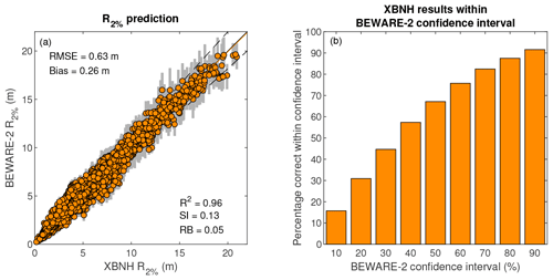
Figure 7 Assessment of R_2 % prediction and confidence intervals. (a) Comparison of R_2 % simulated by XBNH (horizontal axis) and the expected-value prediction of BEWARE-2 (vertical axis) for all validation simulations. Included are the BEWARE-2 50 % prediction confidence interval (vertical gray bands), 1:1 relation (solid black line), 10 % upper and lower deviation from 1:1 (dashed black lines), and linear regression through the data (solid orange line). Model skill metrics refer to those of the expected-value prediction. (b) Percentage of XBNH R_2 % values matching BEWARE-2 predictions within the BEWARE-2 10 %–90 % confidence intervals.

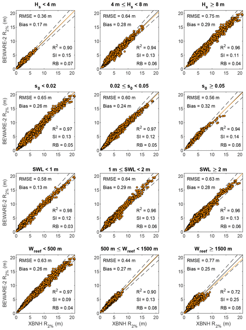
Figure 8 Wave runup simulated by XBNH (horizontal axis) and the expected-value prediction of BEWARE-2 (vertical axis) for variations in the deep-water wave height (top row), deep-water wave steepness (second row), still-water level (third row), and reef width (bottom row). Included are the 1:1 relation (solid black line), 10 % upper and lower deviation from 1:1 (dashed black lines), and linear regression through the data (solid orange line).

In addition to the expected value of R_2 %, BEWARE-2 provides the probability of multiple R_2 % estimates, based on the probability of profile matching (Sect. 2.2.1) and the probabilistic interpolation of oceanic forcing conditions included in the training dataset (Sect. 2.2.2), which can be used to determine empirical R_2 % prediction confidence intervals. The 50 % confidence interval prediction of R_2 % (i.e., 25 %–75 % R_2 % prediction interval) is 26 % ± 12 % (mean and standard deviation) of the expected value of the prediction (Fig. 7, left panel). Whereas 16 % of XBNH R_2 % values in the validation dataset fall exactly within the narrowest 10 % confidence interval (i.e., 45 %–55 % R_2 % prediction interval), 67 % of all XBNH R_2 % values fall within the 50 % confidence interval prediction and 92 % fall within the 90 % confidence interval prediction (Fig. 7, right panel). Again, these values are higher when considering only the 35 normal-reef validation profiles (18 %, 75 %, and 98 %, respectively) than when considering the 13 wide-reef validation profiles (9 %, 49 %, and 75 %, respectively). Note that since the BEWARE-2 confidence intervals were determined empirically from information in the training dataset (as well as the profile-matching procedure) and applied to the validation dataset, rather than derived directly from the validation data, these results are pertinent and provide valuable information for the application of the BEWARE-2 model.

The model skill for the validation cases differs little for variations in oceanic forcing (Fig. 8). The relative measures of model skill R², SI, and RB generally improve marginally for increasing H_s (Fig. 8, top row) and for decreasing s₀ (Fig. 8, second row), whereas RB increases marginally for greater SWL (Fig. 8, third row). For all variations in oceanic forcing conditions, the difference in accuracy is insubstantially smaller than the overall accuracy measures (i.e., difference in SI is approximately 10 %–20 % of the overall SI) and will thus likely not affect the practical application of BEWARE-2. Variation in profile steepness, however, expressed through W_reef (defined as the cross-shore extent between the shoreline and the 15 m depth contour), again highlights the substantially lower R² and higher SI values (i.e., lesser accuracy) for very wide-reef profiles, compared to those of narrow to moderately wide (i.e., W_reef<1500 m) reef profiles (Fig. 8 bottom row).

The skill metrics of BEWARE-2 are relatively insensitive to the selection of the minimum number of iRRPs the target profile is matched to. In sensitivity simulations using between two and six matched iRRP profiles at a minimum (not shown), the median skill metrics for all 49 validation profiles changed by less than 8 %, 11 %, and 1 %, for SI, RB, and R², respectively. For instance, the median SI value for the 49 validation profiles in the sensitivity simulations (SI=0.10–0.12) has less than an 8 % change relative to the median SI value for the standard case of a minimum of four matched iRRPs (SI=0.11).

3.3 Prediction of reef roughness and beach slope effects

The wave runup computed by XBNH for simulations with increased or decreased reef roughness and beach slope is compared to BEWARE-2 predictions of wave runup without and with the use of Eqs. (4) and (8) (“Uncorrected” and “Corrected” columns in Fig. 9, respectively). Application of these correction factors substantially increases predictive skill of BEWARE-2 for the validation profiles, with the RB decreasing by a factor of 1.5–6.5 compared to BEWARE-2 predictions without correction factors.

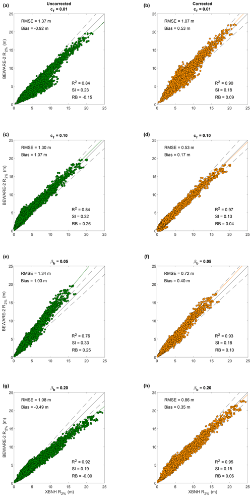
Figure 9 Wave runup simulated by XBNH (horizontal axis) and the expected-value prediction of BEWARE-2 (vertical axis) for variations in the hydrodynamic roughness of the reef (c_f; upper two rows) and beach slope (β_b; lower two rows), without (left panels, green) and with (right panels, orange) the application of Eqs. (4) and (8). Included are the 1:1 relation (solid black line), 10 % upper and lower deviation from 1:1 (dashed black lines), and linear regression through the data (solid green and orange lines).

Application of Eqs. (4) and (8) improves model bias for most validation subsets of oceanic forcing, reef width, reef roughness, and beach slope (indicated by solid orange markers with values closer to zero in Fig. 10). In particular, parameterizing the effect of reef roughness through Eq. (4) most greatly improves model bias for moderate- to high-energy wave events (H_s≥4 m), moderate wave steepness ($\mathrm{0.02}\le s_{\mathrm{0}}<\mathrm{0.05}$), low water levels (SWL<1 m), and moderate- to wide-reef profiles (W_reef≥500 m). Conversely, parameterizing the effect of beach slope through Eq. (8) most greatly improves model bias for low wave steepness (s₀<0.02), high water levels (SWL≥2 m), and narrower-reef profiles (W_reef<500 m).

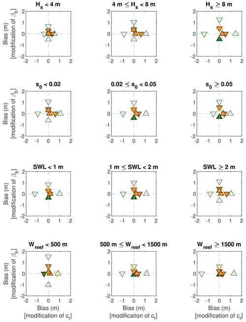
Figure 10 Bias in BEWARE-2 wave runup for simulations with increased (△) or decreased (▿) reef roughness (c_f; horizontal axis) and beach slope (β_b; vertical axis). Markers are shown for simulations without (green) and with (orange) the use of Eqs. (4) and (8). Solid green markers indicate that the result without the use of Eqs. (4) and (8) has the lowest absolute bias value, whereas solid orange markers indicate less bias with the use of Eqs. (4) and (8). Results are grouped by the deep-water wave height (top row), deep-water wave steepness (second row), still-water level (third row), and reef width (bottom row).

Equations (4) and (8) do, however, systematically overpredict wave runup (also shown in Fig. 9). In certain cases, this overprediction may (in an absolute sense) be greater than the underprediction of the uncorrected BEWARE-2 results (indicated in Fig. 10 by solid green markers). In particular, this is the case for the application of Eq. (8) on steep beach profiles (β_b=0.20) in combination with high-energy wave events (H_s≥8 m), moderate to steep waves (s₀≥0.02), low to moderate water levels (SWL<2 m), or moderate- to wide-reef profiles (W_reef≥500 m). With respect to the application of Eq. (4), deterioration in bias is found only for the validation subset with narrower-reef profiles (W_reef<500 m), in combination with decreased reef roughness (c_f=0.01). Note that application of Eqs. (4) and (8) improves model bias for all oceanic forcing conditions and reef widths in the case of increased reef roughness (c_f=0.10) and milder beach slopes (β_b=0.05).

4 Discussion

BEWARE-2 was developed to provide a quick, accurate prediction of wave-driven total water levels (setup plus runup) across a wide range of extrinsic oceanographic forcing conditions (SWL, H_s,0, and T_p) and intrinsic coastal morphological parameters (reef bathymetry, c_f, and β_b). Over a range of 4 m in SWL, 10 m in H_s,0, and 16 s in T_p across the 48 validation profiles (spanning the range of reef morphologies in seven geographic regions), the meta-process modeling system produced results with an RMSE of 0.63 m and SI of 0.13, with 67 % of all R_2 % values falling within the 50 % confidence interval prediction and 92 % falling within the 90 % confidence interval prediction of the full, process-based hydrodynamic XBNH model. Incorporating modifications into the modeling system to account for variations in c_f and β_b allows for systematic errors (RB) in BEWARE-2 predictions to be reduced by a factor of 1.5–6.5. Once having been trained, this relatively accurate solution is provided by the BEWARE-2 meta-process modeling system computationally faster by 4–5 orders of magnitude (i.e., 𝒪(10⁻²) s per R_2 % prediction) than the full, process-based hydrodynamic XBNH model (𝒪(10²–10³) s per R_2 % prediction) on a standard desktop computer.

4.1 Benefits and limitations of the BEWARE-2 model

A key advantage of the BEWARE-2 meta-process modeling system is its ability to estimate uncertainties in the computed runup metrics. The uncertainty range is given by the range of weighted runup results obtained from the XBNH model simulations for the matched RRPs and the nearest (upper and lower) oceanic forcing conditions (SWL, H_s,0, and T_p). This indication of uncertainty in the computed runup metric (i.e., R_2 %) would require multiple simulations and post-processing in a deterministic approach, which would come at great computational cost. However, in this implementation, the accuracy of the meta-process modeling system should not be expected to be greater than that of the underlying process-based model.

The XBNH model is reasonably well validated, as described in the Introduction and Methods, but it is not perfect. A key limitation of BEWARE-2 is the one-dimensional nature of the underlying XBNH model simulations and thus the meta-process model dataset, which is unlikely to be very accurate in highly two-dimensional situations, such as in the presence of reef channels (e.g., Storlazzi et al., 2022). In addition, BEWARE-2 shows notably lower skill in reproducing XBNH runup values for very wide-reef profiles (characteristic of barrier and extremely wide fringing reefs), likely due to the relatively low profile coverage (only 20 RRPs) and large number of possible permutations. Although this may be improved by including a greater number of wide RRPs in the dataset, the real-world accuracy of the underlying XBNH model may likely be lower for very wide-reef profiles than other reefs for which it has been validated, as one-dimensional XBNH models are unable to account for wind growth of waves or large-scale topographic refraction (Scott et al., 2020). Further extension of BEWARE-2 for these reef types is therefore currently constrained by the inherent uncertainty in applying XBNH to very wide-reef profiles. A final key limitation of BEWARE-2 is the underlying reef profile dataset, which is heavily biased toward data from US (fringing) coral-reef-lined coasts (due to consistent lidar data availability at the time of BEWARE-2 development) and may lack other important characteristic reef profiles such as those of barrier and platform reefs. The collection and dissemination of accurate, high-resolution bathymetric data at other coral-reef-lined coasts around the world would greatly aid in the application of BEWARE-2, as well as other process-based meta-models, in global efforts to reduce the impacts of coastal flooding.

4.2 Potential applications of BEWARE-2

The BEWARE-2 meta-process modeling system is fast enough for large-scale application in EWSs. As noted by Winter et al. (2020), a coastal-flooding EWS would require four main modules: sea levels (including tides and non-tidal residuals), offshore wave conditions, nearshore waves and water levels, and coastal flooding. BEWARE-2 can use the output of global or regional tide models (based on tide station observations and/or satellite altimetry, e.g., TPXO; Egbert and Erofeeva, 2002), global (e.g., HYCOM; Halliwell et al., 1998) or regional general circulation models, or a mix of these models as SWL input. Offshore wave conditions (H_s,0 and T_p) for BEWARE-2 can be provided by operational global wave models, such as NOAA GEFS-Wave (utilizing the WAVEWATCH III spectral wave model of Tolman, 2009) or region-specific alternatives. Using these oceanographic inputs, BEWARE-2 provides runup and, in the future, potentially nearshore waves, water levels, and overtopping volumes that can be used to assess coastal flooding and thus form the core of an EWS for reef-lined coasts. The primary computational cost of developing an EWS based on BEWARE-2 is pre-processing – developing the BEWARE-2 database and matching measured reef profiles to the RRPs. Once the desired real-world reef profiles have been assigned to the RRPs and the BEWARE-2 database has been linked to the operational water level and wave forecasts, the modeling system can provide a statistical value (e.g., R_2 %) of runup and measures of its confidence within seconds.

BEWARE-2 can also provide a very rapid first approximation of runup and flooding potential for use in flood risk analyses. In such analyses, the influence of reef health (here expressed in terms of reef roughness following Quataert et al., 2015, and Norris et al., 2023) on runup and hence flood risk can be calculated using the BEWARE-2 reef roughness parameterization. Due to the speed of the system, BEWARE-2 can be used to simulate hundreds of years of runup on a range of profiles with varying reef health to allow for climate hindcast and future climate scenario analysis of wave runup. This could help identify coastlines at particular risk of higher and/or more frequent wave runup in the future. Alternatively, BEWARE-2 results can be used to identify relevant nearshore wave and water level conditions in long time series for simulation in other more computationally expensive numerical models (e.g., Masselink et al., 2020, 2021).

4.3 Next steps

The BEWARE-2 meta-process modeling system and the underlying process-based hydrodynamic XBNH model ultimately require field validation of both waves and water levels over reefs and the resulting wave-driven runup on the coast. Such measurements, especially runup, are scarce but are slowly increasing with the deployment of coastal imaging systems, such as Argus (Holman and Stanley, 2007), in tropical, reef-lined locations. Further testing should also include profiles from non-US reefs that are not included in the dataset used to develop the RRPs, prior to application in other regions.

One of the great aspects of the BEWARE-2 database is its modular nature. The range of oceanographic forcing conditions can be expanded (lower or higher water level and/or wave heights and periods) or refined by additional XBNH simulations. Non-US reef profiles that are morphologically distinct from the current dataset can be included through the addition of new RRPs. Similarly, if one wanted to investigate the role of coral reef restoration in the reef profiles, new RRPs that include the effects of restoration (changes in height and/or bed roughness) could be simulated in XBNH (e.g., Roelvink et al., 2021) and added to the database. Lastly, one could utilize information in the BEWARE-2 dataset to extend prediction variables with output such as overtopping volumes for use in coastal flood modeling studies.

5 Conclusions

A surrogate, meta-process model (BEWARE-2) of the process-based hydrodynamic model XBeach Non-Hydrostatic (XBNH; de Ridder et al., 2021) has been developed to estimate wave runup on morphologically diverse reefs. BEWARE-2 builds on work by Pearson et al. (2017) and Scott et al. (2020) to account for a broad range of oceanic forcing conditions (water levels, wave height, and period), diverse morphologies of naturally occurring coral reef profiles, and variations in reef roughness and beach slope.

The BEWARE-2 meta-process model accurately reproduces runup (2 % exceedance runup level; R_2 %) simulated by the process-based XBNH model on 48 real-world profiles drawn from seven geographic regions. BEWARE-2 was tested for 100 oceanic forcing conditions (combinations of the offshore water level, wave height, and period), with simulated runup ranging from 0.17 to 20.9 m. BEWARE-2 was shown to have a high overall coefficient of determination (R²=0.96) and an overall root mean square error of 0.63 m (scatter index of 0.13) and bias of 0.26 m (relative bias of 0.05). Model skill differed little for variations in oceanic forcing conditions but was substantially greater for profiles with reef widths less than 1.5 km (R²=0.98, scatter index = 0.10, relative bias = 0.05) than for wider-reef profiles (R²=0.72, scatter index = 0.25, relative bias = 0.08). Parametric extensions to BEWARE-2 to account for variations in reef roughness and beach slope were shown to reduce systematic errors (relative bias) in BEWARE-2 predictions by a factor of 1.5–6.5 for relatively coarse or smooth reefs and mild or steep beach slopes.

The simulation of wave runup using BEWARE-2 is faster by 4–5 orders of magnitude (𝒪(10⁻²) s per R_2 % prediction) than simulating runup using XBNH (𝒪(10²–10³) s per R_2 % prediction). In addition, the framework of the BEWARE-2 meta-process model provides a probability distribution of wave runup that can be used to determine the expected value of R_2 %, alongside confidence bands around this prediction. Key limitations of BEWARE-2 are related to the one-dimensional nature of underlying XBNH model simulations, for application both in highly two-dimensional situations and for very wide-reef profiles, as well as the underlying reef profile dataset, which is heavily biased toward data from US coral-reef-lined coasts.

The accuracy and speed of the BEWARE-2 meta-process model suggest that it may be a useful tool for early-warning systems and current and future coastal flood risk analysis.

Appendix A: Accounting for variations in reef roughness and beach slope

A1 Calibration dataset

In an approach similar to the creation of the BEWARE-2 training dataset (Sect. 2.1.3), a separate and substantially smaller dataset was created for the purpose of developing and calibrating BEWARE-2 wave runup correction factors for smoother and rougher reefs and steeper and milder beach slopes. To this end, XBNH simulations were carried out on 31 morphologically diverse reef profiles (Fig. A1) that were selected through agglomerative hierarchical clustering of the 530 normal-reef iRRPs and that represent a subset of the BEWARE-2 RRPs. XBNH simulations were forced using a subset of the hydrodynamic boundary conditions included in the BEWARE-2 training dataset (Table A1). XBNH simulations for all calibration reef profiles and hydraulic boundary conditions were run with the reference reef roughness ($c_{\mathrm{f},\mathrm{ref}}=\mathrm{0.05}$) and beach slope (${\mathit{\beta }}_{\mathrm{b},\mathrm{ref}}=\mathrm{0.10}$), as well as for higher (c_f=0.10) or lower (c_f=0.01) reef roughness or steeper (β_b=0.20) or milder (β_b=0.05) beach slope (i.e., five c_f–β_b combinations in total). Other XBNH model parameters were set equal to those used for the BEWARE-2 training dataset (Sect. 2.1.2). XBNH R_2 % values for the calibration dataset were calculated as described in Sect. 2.1.3.

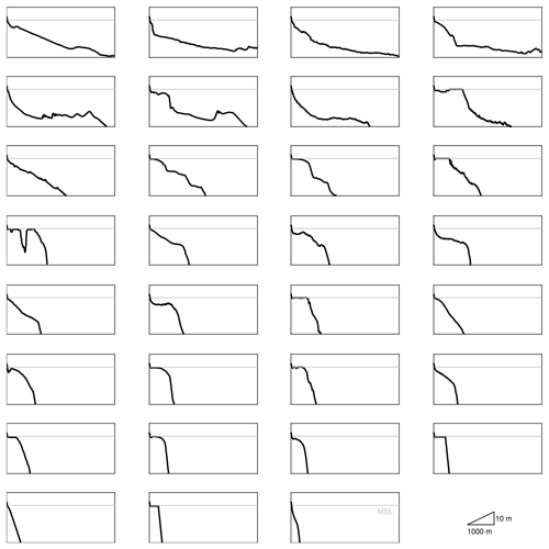
Figure A1 Cross-shore profiles of 31 morphologically diverse RRP reef transects derived by agglomerative hierarchical clustering used to calibrate the parameterization of bed roughness and beach slope effects on wave runup.

Table A1 Overview of hydrodynamic forcing conditions used for the calibration of reef roughness and beach slope effects on wave runup. *Wave height combinations for T_p=8 s are constrained by maximum deep-water wave steepness.

A2 Parameterization of the reef roughness effect

The effect of increased or reduced roughness of the reef relative to c_f,ref on wave runup is not included in the underlying dataset of BEWARE-2. Instead, this effect is parameterized in the model through the estimation of the relative increase or decrease in wave height at the toe of the beach due to roughness effects, under the assumption that changes in wave runup will be proportional to changes in the wave height reaching the beach:

$$\begin{array}{}\text{(A1)}& \mathrm{\Delta }{R}_{\mathrm{2}\mathit{\%}}\propto \mathrm{\Delta }{H}_{\mathrm{beach}\mathrm{toe}}.\end{array}$$

To estimate the contribution of reef roughness effects on the wave height at the beach toe (defined as the landward edge of the reef located at a depth of 0.5 m; see Sect. 2.1.2), we assume a stationary wave energy balance on the reef profile:

$$\begin{array}{}\text{(A2)}& {\displaystyle \frac{\partial c_{\mathrm{g}}\left(x\right)E\left(x\right)}{\partial x}}-D_f\left(x\right),\end{array}$$

in which E is the wave energy, c_g is the wave group velocity, x is the cross-shore coordinate, $D_{\mathrm{f}}\left(x\right)=\frac{\mathrm{2}}{\mathrm{3}\mathit{\pi }}{c}_{\mathrm{f}}\mathit{\rho }{u}_{\mathrm{orb}}^{\mathrm{3}}\left(x\right)$ is the wave dissipation term due to reef roughness effects, ρ is the density of water, and u_orb is the near-bed wave orbital velocity. Note that dissipation due to depth-induced breaking is intentionally not included in Eq. (A2) but is instead imposed as a boundary condition to the solution in Eq. (A9).

Through linearization of the wave group velocity in Eq. (A2), the integrated wave energy loss across the reef due to reef roughness effects only (ΔE_r) is approximated by

$$\begin{array}{}\text{(A3)}& \mathrm{\Delta }{E}_{\mathrm{r}}\approx -\underset{L_{c_{\mathrm{f}}}}{\int }{\displaystyle \frac{D_{\mathrm{f}}\left(x\right)}{c_{\mathrm{g}}\left(x\right)}}\mathrm{d}x,\end{array}$$

in which $L_{c_{\mathrm{f}}}$ is the cross-shore extent of the model domain that has a hydrodynamic roughness value equal to c_f,ref, i.e., the cross-shore extent of the coral reef.

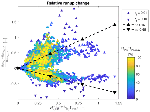
Figure A2 Variation in relative wave runup as a function of the right-hand term of Eq. (A6). Linear proportionality constants α_r found for reef profiles with lower (c_f=0.01; ▴) and higher (c_f=0.10; ▾) reef roughness are shown as dashed lines. Computed relative runup values are colored by the computed wave runup relative to the maximum runup in the calibration dataset.

Given $H=\sqrt{\frac{\mathrm{8}E}{\mathit{\rho }g}}$, the wave height loss across the reef due to reef roughness effects only (ΔH_r) is proportional to

$$\begin{array}{}\text{(A4)}& \mathrm{\Delta }{H}_{\mathrm{r}}\propto -\sqrt{{\displaystyle \frac{c_{\mathrm{f}}}{g}}}{\mathrm{\Gamma }}_{\mathrm{reef}},\end{array}$$

where Γ_reef is the integrated wave dissipation estimate defined in Eq. (7) and repeated below in Eq. (A5).

$$\begin{array}{}\text{(A5)}& {\mathrm{\Gamma }}_{\mathrm{reef}}=\sqrt{\underset{L_{c_{\mathrm{f}}}}{\int }{\displaystyle \frac{u_{\mathrm{orb}}^{\mathrm{3}}\left(x\right)}{c_{\mathrm{g}}\left(x\right)}}\mathrm{d}x}\end{array}$$

The assumed proportionality of Eq. (A1) is combined with the estimated difference in wave height loss across the reef due to varying reef roughness, normalized by the offshore significant wave height (H_s,0), to derive a proportionality for relative variations in wave runup due to reef roughness effects:

$$\begin{array}{}\text{(A6)}& {\displaystyle \frac{R_{\mathrm{2}\mathit{\%},c_{\mathrm{f}}}-R_{\mathrm{2}\mathit{\%},c_{\mathrm{f},\mathrm{ref}}}}{R_{\mathrm{2}\mathit{\%},c_{\mathrm{f},\mathrm{ref}}}}}\propto {\displaystyle \frac{\sqrt{\frac{\mathrm{1}}{g}}\sqrt{|\frac{c_{\mathrm{f}}}{c_{\mathrm{f},\mathrm{ref}}}-\mathrm{1}|}{\mathrm{\Gamma }}_{\mathrm{reef}}}{H_{\mathrm{s},\mathrm{0}}}}={\displaystyle \frac{\sqrt{\frac{\mathrm{1}}{g}}{\mathit{\gamma }}_{\mathrm{r}}{\mathrm{\Gamma }}_{\mathrm{reef}}}{H_{\mathrm{s},\mathrm{0}}}},\end{array}$$

where $R_{\mathrm{2}\mathit{\%},c_{\mathrm{f},\mathrm{ref}}}$ is the wave runup computed for the reference reef roughness value ($c_{\mathrm{f},\mathrm{ref}}=\mathrm{0.05}$) using the underlying XBNH dataset, $R_{\mathrm{2}\mathit{\%},c_{\mathrm{f}}}$ is the estimated wave runup for reef profiles with a higher or lower roughness (c_f) than the reference roughness, and ${\mathit{\gamma }}_{\mathrm{r}}=\sqrt{|\frac{c_{\mathrm{f}}}{c_{\mathrm{f},\mathrm{ref}}}-\mathrm{1}|}$ is the relative reef roughness coefficient defined in Eq. (6).

Solving the right-hand term in Eq. (A6) requires an estimate of the local near-bed wave orbital velocity, which is computed as

$$\begin{array}{}\text{(A7)}& u_{\mathrm{orb}}\left(x\right)={\displaystyle \frac{\mathit{\pi }{H}_{\mathrm{rms}}\left(x\right)}{T_{\mathrm{p}}}}{\displaystyle \frac{\mathrm{1}}{\sinh \left(k_{\mathrm{p}}\left(x\right)h_{\mathrm{0}}\left(x\right)\right)}},\end{array}$$

where H_rms is the root mean square wave height, k_p is the wave number based on T_p, and h₀ is the local water depth estimated using the cross-shore profile elevation and the offshore still-water level (SWL).

The root mean square wave height at the offshore boundary of the reef profile (H_rms,0) is estimated as

$$\begin{array}{}\text{(A8)}& H_{\mathrm{rms},\mathrm{0}}={\displaystyle \frac{H_{\mathrm{s},\mathrm{0}}}{\sqrt{\mathrm{2}}}}.\end{array}$$

Wave height transformation across the reef profile is estimated using a forward-marching scheme, starting at the offshore boundary of the profile. In doing this, the computed wave height includes wave shoaling and depth-induced breaking processes but intentionally neglects dissipation due to hydrodynamic bed roughness:

$$\begin{array}{}\text{(A9)}& \begin{array}{rl}{H}_{\mathrm{rms}}\left(x\right(i\left)\right)=& \min \left(H_{\mathrm{rms}}\left(x\right(i-\mathrm{1}\left)\right)\sqrt{{\displaystyle \frac{c_{\mathrm{g},\mathrm{p}}\left(x\right(i-\mathrm{1}\left)\right)}{c_{\mathrm{g},\mathrm{p}}\left(x\right(i\left)\right)}}},\right.\\ & \left.{\mathit{\gamma }}_{\mathrm{b}}{h}_{\mathrm{0}}\left(x\right(i\left)\right)\right)\end{array}\end{array}$$

where i is the numerical grid cell counter, starting at i=1 at the offshore boundary and increasing in the cross-shore direction; c_g,p is the wave group velocity estimated using T_p; and γ_b=0.78 is the wave breaker index.

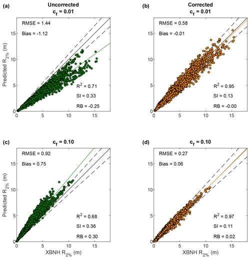
Figure A3 Wave runup predicted by BEWARE-2, without (a, c) and with (b, d) use of α_r, relative to that simulated by XBNH for smoother (c_f=0.01; a, b) and rougher (c_f=0.10; c, d) reefs than the reference reef roughness ($c_{\mathrm{f},\mathrm{ref}}=\mathrm{0.05}$) in the calibration dataset. Included are the 1:1 relation (solid black line), 10 % upper and lower deviation from 1:1 (dashed black lines), and linear regression through the data (solid green and orange lines).

Equation (A9) allows for a first-order estimate of wave heights across the reef in the absence of reef roughness effects. Although this method neglects important physical processes (e.g., wave setup, infragravity wave generation), we find that this first-order estimate provides sufficient information with which to derive proportionality constants for Eq. (A6) and subsequently improve predictions of wave runup on reef profiles with greater and lesser roughness (Sect. 3.3).

Linear proportionality coefficients (α_r) for Eq. (5) (and Eq. A6) are found separately for relatively smooth (c_f=0.01) and rough (c_f=0.10) reef profiles by computing the left-hand and right-hand terms of Eq. (A6) for the reef roughness calibration simulations described in Appendix A1 and fitting linear least-square error relations to the smooth- and rough-reef datasets (Fig. A2). In this manner, we find proportionality coefficients ${\mathit{\alpha }}_{\mathrm{r},\mathrm{smooth}}=\mathrm{1.16}$ for relatively smooth reefs and ${\mathit{\alpha }}_{\mathrm{r},\mathrm{rough}}=-\mathrm{0.65}$ for relatively rough reefs, with considerable scatter around the linear fit that is likely due to the extensive simplification of the true hydrodynamics on reef profiles.

Despite the high degree of simplification present in this methodology, application of the calibrated α_r coefficients to the conditions included in the calibration dataset (Appendix A1) greatly improves skill metrics of wave runup (Fig. A3). In particular, application of the calibrated coefficients greatly reduces the bias of the runup predictions (i.e., improvement of RB from −0.25 to 0.00 for smoother reefs and from 0.30 to 0.02 for rougher reefs), as would be expected from the linear-fit methodology. Importantly, as shown in Sect. 3.3, application of the calibrated α_r coefficients to the validation dataset also substantially reduces model bias and improves the wave runup skill metrics of BEWARE-2.

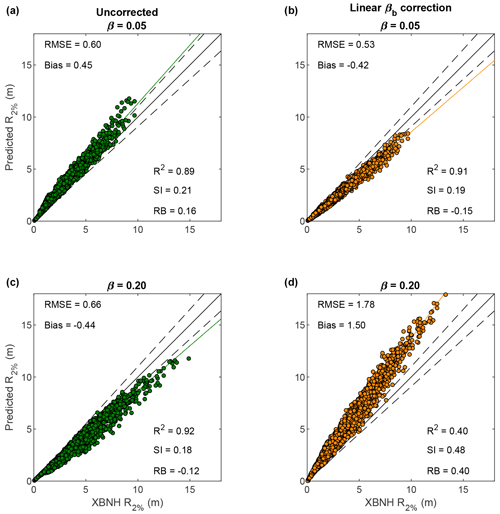
Figure A4 Wave runup predicted by BEWARE-2 relative to that simulated by XBNH for milder (a, b) and steeper (c, d) beach slopes than the reference beach slope (${\mathit{\beta }}_{\mathrm{b},\mathrm{ref}}=\mathrm{0.10}$) in the calibration dataset. Predictions are without beach slope correction (a, c) and with a correction factor α_b linearly proportional to β_b (κ_b=1). Note the detrimental effect of the linear beach slope correction on the model skill in panel (d).

The two derived values of α_r appear to scale approximately proportionally with the square root of the change in the reef roughness coefficient $\left({\mathit{\alpha }}_{\mathrm{r},\mathrm{smooth}}\approx \mathrm{0.5}\sqrt{\frac{\mathrm{0.05}}{\mathrm{0.01}}};{\mathit{\alpha }}_{\mathrm{r},\mathrm{rough}}\approx -\mathrm{0.5}\sqrt{\frac{\mathrm{0.10}}{\mathrm{0.05}}}\right)$, with a change in sign for rougher reefs relative to the reference reef roughness. However, the use of interpolated or extrapolated values of α_r for reefs with other representative roughness values is not recommended without further investigation of this relation. Instead, wave runup values computed in BEWARE-2 using α_r,smooth and α_r,rough can be used to illustrate likely upper and lower bounds of wave runup for natural reefs in poor or good health.

A3 Parameterization of the beach slope variation effect

Similarly to reef roughness variations, the effect of steeper or milder beach slopes relative to β_b,ref on wave runup is not included in the underlying dataset of BEWARE-2. Instead, this effect is parameterized in the model through estimation of the contribution of the beach slope to the incident-band swash and swash-zone setup.

Following Stockdon et al. (2006), we can describe the components of wave runup as

$$\begin{array}{}\text{(A10)}& R_{\mathrm{2}\mathit{\%}}=c_{\mathrm{R}}\left(\stackrel{\mathrm{‾}}{{\mathit{\eta }}_{\mathrm{wl}}}+{\displaystyle \frac{\sqrt{S_{\mathrm{IG}}^{\mathrm{2}}+S_{\mathrm{inc}}^{\mathrm{2}}}}{\mathrm{2}}}\right),\end{array}$$

where $\stackrel{\mathrm{‾}}{{\mathit{\eta }}_{\mathrm{wl}}}$ is the time-averaged vertical position of the waterline observed at the shore; S_IG and S_inc are the infragravity and incident-band swash, respectively; and c_R is a regression coefficient found to have a value of 1.1 in the data of Stockdon et al. (2006).

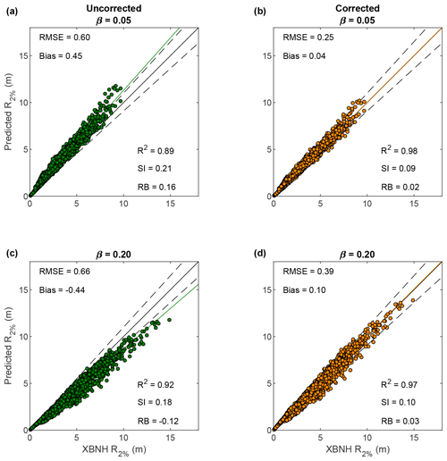
Figure A5 Wave runup predicted by BEWARE-2 relative to that simulated by XBNH for milder (a, b) and steeper (c, d) beach slopes than the reference beach slope (${\mathit{\beta }}_{\mathrm{b},\mathrm{ref}}=\mathrm{0.10}$) in the calibration dataset using ${\mathit{\kappa }}_{\mathrm{b}}=\frac{\mathrm{1}}{e}$.

Following Stockdon et al. (2006), we assume that variation in beach slope (in this case ${\mathit{\beta }}_{\mathrm{b}}=\mathrm{0.05}-\mathrm{0.20}$) will not affect S_IG. Furthermore, we assume that the contribution of the surf-zone setup ($\stackrel{\mathrm{‾}}{{\mathit{\eta }}_{\mathrm{surf}}}$) to the setup observed at the shoreline ($\stackrel{\mathrm{‾}}{{\mathit{\eta }}_{\mathrm{wl}}}$) is independent of the beach slope (but instead dependent upon the shoreface and reef profile) and therefore already correct in the underlying training dataset for BEWARE-2. It remains clear, however, that a beach slope correction factor (α_b) is likely required for the incident-band swash (S_inc) and setup occurring within the swash zone ($\stackrel{\mathrm{‾}}{{\mathit{\eta }}_{\mathrm{swash}}}=\stackrel{\mathrm{‾}}{{\mathit{\eta }}_{\mathrm{wl}}}-\stackrel{\mathrm{‾}}{{\mathit{\eta }}_{\mathrm{surf}}}$) to improve wave runup predictions in BEWARE-2 for beach slopes different than β_b,ref.

To determine the value of α_b we first empirically determine the values of R_2 %, $\stackrel{\mathrm{‾}}{{\mathit{\eta }}_{\mathrm{wl}}}$, S_IG, and S_inc from the time series of the waterline elevation (i.e., time-varying swash signal) output by XBNH in all calibration simulations with the reference beach slope (${\mathit{\beta }}_{\mathrm{b},\mathrm{ref}}=\mathrm{0.10}$). In doing this, we compute R_2 % as the empirical 2 % exceedance height of swash peaks above the still-water level and S_IG and S_inc from the variance density spectrum of the simulated waterline elevation time series (see, e.g., Stockdon et al., 2006; de Beer et al., 2021) using frequency integration limits of $\frac{\mathrm{1}}{\mathrm{20}}{f}_{\mathrm{p}}\le f<\frac{\mathrm{1}}{\mathrm{2}}{f}_{\mathrm{p}}$ for the computation of S_IG and $\frac{\mathrm{1}}{\mathrm{2}}{f}_{\mathrm{p}}\le f<\mathrm{3}{f}_{\mathrm{p}}$ for the computation of S_inc, where f is frequency and $f_{\mathrm{p}}=\frac{\mathrm{1}}{T_{\mathrm{p}}}$ is the offshore wave spectral peak frequency. We derive $\stackrel{\mathrm{‾}}{{\mathit{\eta }}_{\mathrm{surf}}}$ from the mean water level at the nearest XBNH model output point to the toe of the beach, which is located at 0.5 m b.m.s.l. (below mean sea level), and $\stackrel{\mathrm{‾}}{{\mathit{\eta }}_{\mathrm{swash}}}$ from the time-averaged waterline elevation. We subsequently calculate the value of c_R separately for every simulation as $c_{\mathrm{R}}=\frac{R_{\mathrm{2}\mathit{\%}}}{\stackrel{\mathrm{‾}}{{\mathit{\eta }}_{\mathrm{wl}}}+\frac{\sqrt{S_{\mathrm{IG}}^{\mathrm{2}}+S_{\mathrm{inc}}^{\mathrm{2}}}}{\mathrm{2}}}$, thereby ensuring that application of Eq. (A10) with simulation-specific values of c_R provides an exact representation of the waterline time-series-derived R_2 % value. The values of c_R computed in this manner range between 0.92 and 2.04 (median value of 1.16).

Table A2 Overview of profile-matching properties and model skill values for the 48 validation profiles. Matching properties include the number of probabilistically matched RRPs (N_match) and the maximum matching probability (p_max), and skill values include the root mean square error (RMSE), model bias (bias), scatter index (SI), relative bias (RB), and coefficient of determination (R²) of the BEWARE-2 wave runup prediction.

Given the computed values of c_R, $\stackrel{\mathrm{‾}}{{\mathit{\eta }}_{\mathrm{surf}}}$, $\stackrel{\mathrm{‾}}{{\mathit{\eta }}_{\mathrm{swash}}}$, S_IG, and S_inc for all calibration simulations with the reference beach slope β_b,ref, we can estimate the wave runup for other beach slopes ($R_{\mathrm{2}\mathit{\%}}^{\mathrm{m},\mathrm{b}}$) through inclusion of α_b in Eq. (A10) as follows:

$$\begin{array}{}\text{(A11)}& R_{\mathrm{2}\mathit{\%}}^{\mathrm{m},\mathrm{b}}=c_{\mathrm{R}}\left(\stackrel{\mathrm{‾}}{{\mathit{\eta }}_{\mathrm{surf}}}+{\mathit{\alpha }}_{\mathrm{b}}\stackrel{\mathrm{‾}}{{\mathit{\eta }}_{\mathrm{swash}}}+{\displaystyle \frac{\sqrt{S_{\mathrm{IG}}^{\mathrm{2}}+{\left({\mathit{\alpha }}_{\mathrm{b}}{S}_{\mathrm{inc}}\right)}^{\mathrm{2}}}}{\mathrm{2}}}\right).\end{array}$$

To test the validity of Eq. (A11), values of $R_{\mathrm{2}\mathit{\%}}^{\mathrm{m},\mathrm{b}}$ are compared to runup values derived empirically from XBNH simulations for the same RRPs and forcing conditions but with the beach slope set to β_b=0.05 and β_b=0.20 (see Sect. A1).

As Stockdon et al. (2006) found both $\stackrel{\mathrm{‾}}{{\mathit{\eta }}_{\mathrm{wl}}}$ and S_inc to be proportional to β_b, the required beach slope correction factor α_b would be expected to be proportional to the change in beach slope relative to the reference beach slope (i.e., ${\mathit{\alpha }}_{\mathrm{b}}=\frac{{\mathit{\beta }}_{\mathrm{b}}}{{\mathit{\beta }}_{\mathrm{b},\mathrm{ref}}}$). However, we find that if a linear relation between β_b and α_b is used, Eq. (A11) greatly overestimates the effect of the beach slope on wave runup relative to that simulated by XBNH, showing an underestimation of wave runup relative to XBNH for milder beach slopes (Fig. A4, top right panel) and overestimation for steeper beach slopes (Fig. A4, bottom right panel). In a quantitative sense, application of Eq. (A11) and a linear relation between β_b and α_b even reduces the predictive skill of the model for steep beach slopes (β_b=0.20) relative to applying no beach slope correction at all (Fig. A4, bottom panels).

Substantial improvement in model predictive skill is found, however, if a non-linear relation is assumed to be between β_b and α_b in the form of ${\mathit{\alpha }}_{\mathrm{b}}={\left(\frac{{\mathit{\beta }}_{\mathrm{b}}}{{\mathit{\beta }}_{\mathrm{b},\mathrm{ref}}}\right)}^{{\mathit{\kappa }}_{\mathrm{b}}}$. Through minimization of the combined relative bias (RB) of the runup prediction for both milder and steeper beach slopes, optimal values of κ_b were found in the range of 0.35–0.38 (difference in combined RB across the range of less than 0.5 percentage points), with a value ${\mathit{\kappa }}_{\mathrm{b}}=\frac{\mathrm{1}}{e}\approx \mathrm{0.37}$ selected for application in the model (Eq. 10).

Application of Eq. (8) using ${\mathit{\kappa }}_{\mathrm{b}}=\frac{\mathrm{1}}{e}$ substantially improves the skill of BEWARE-2 in reproducing XBNH wave runup on milder and steeper beaches in the calibration dataset (see Fig. A5). The non-linear nature of Eq. (10) is, however, not fully understood, and extrapolation for beach slopes outside the range of the calibration simulations (i.e., β_b=0.05–0.20) is therefore not recommended.