Influence of data source and copula statistics on estimates of compound flood extremes in a river mouth environment

Coastal and riverine floods are major concerns worldwide as they can impact highly populated areas and result in significant economic losses. In a river mouth environment, interacting hydrological and oceanographical processes can enhance the severity of floods. The compound flood hazards from high sea levels and high river discharge are often estimated using copulas, among other methods. Here, we systematically investigate the influence of different data sources coming from observations and models as well as the choice of copula on extreme water level estimates. While we focus on the river mouth at the city of Halmstad (Sweden), the approach presented is easily transferable to other sites. Our results show that the choice of data sources can considerably impact the results up to 10 % and 15 % for the river time series and 3 % to 4.6 % for the sea level time series under the 5- and 30-year return periods, respectively. The choice of copula can also strongly influence the outcome of such analyses up to 13 % and 9.5 % for the 5-year and 30-year return periods. Each percentage refers to the normalized difference in return level results we can expect when choosing a certain copula or input dataset. The copulas found to statistically best fit our datasets are the Clayton, BB1, and Gaussian (once) ones. We also show that the compound occurrence of high sea levels and river runoff may lead to heightened flood risks as opposed to considering them independent processes and that, in the current study, this is dominated by the hydrological driver. Our findings contribute to framing existing studies, which typically only consider selected copulas and datasets, by demonstrating the importance of considering uncertainties.

1 Introduction

Floods can cause severe damage to infrastructure and disrupt activities in harbours and coastal communities. Flooding can result from meteorological, hydrological, and oceanographic sources such as storm surges, extreme river runoff, or precipitation. Storm surges correspond to seawater being pushed by the wind stress and the barometric pressure effect under deep low-pressure weather systems. Heavy precipitation can form under different conditions such as intense cyclonic activity, sometimes during the same deep low-pressure systems that cause the storm surge or sometimes during convective weather conditions. River runoff can also have different origins, such as snow melting upstream or intense precipitation, related to the same large-scale weather system that could cause the storm surge or separately. Hence, several processes could contribute to compound effects and independently cause damage and disruption to activities in the coastal zone. River runoff and precipitation may take some time to drain into the sea, and the flow from land to the sea can therefore be slowed down or even momentarily become blocked when storm surges happen (Wahl et al., 2015). This process can be referred to as coastal backwater effects, while the water level at the river mouth increases due to high river discharge or high sea level or compounding effects (Feng et al., 2022).

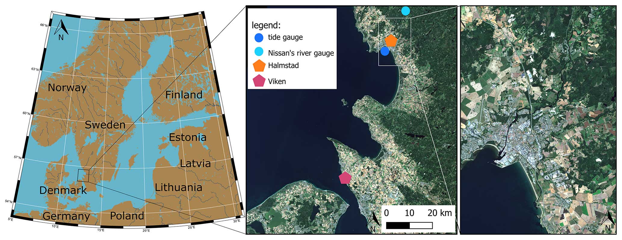
Figure 1 Regional map of southern and central Sweden with a zoom around our study area and the city of Halmstad (Pawlowicz, 2020; Sentinel-2 cloudless, 2021).

Settlements and infrastructure located in river mouth environments are inherently susceptible to all of the above. The combination of multiple factors, extreme or not, happening at the same place simultaneously, successively, or consecutively can potentially lead to larger compounded floods and more severe impacts on the environment and society. Compound flooding can also result when preceding conditions amplify the impact of the event (Andrée et al., 2023; Zscheischler et al., 2020; AghaKouchak et al., 2020). Even if trends over the last 40 to 60 years are estimated with high uncertainty, it is likely that extremes including compound events will become more severe in northern Europe with the changing climate (Rutgersson et al., 2022).

Couasnon et al. (2020) highlight the importance of considering interactions, referring to their co-occurrence probabilities between river discharge and storm surge extremes in river mouth environments. They demonstrate that dependencies between these drivers are not random and may result from relations between weather systems at the synoptic scale with local conditions such as the topography. Ward et al. (2018) study the dependence between river discharge and skew surge at the global scale, where significant dependency is found in several stations in Europe, mainly located around the UK coastline. Hendry et al. (2019) also highlighted those dependencies around the UK coast and linked the spatial variability found with differences in storm characteristics. In northwestern Europe, it has been shown that the fluvial flood hazard increases with high sea levels and stronger storms, and this may be critical in populated and low-elevation coastal areas (Ganguli and Merz, 2019a). Increasing trends within the last decades in the magnitude and frequency of coastal compound floods between river discharge and sea levels are found for gauges between 47 and 60° N latitude, while decreasing trends are highlighted for gauges >60° N in northwestern Europe (Ganguli and Merz, 2019b), where rare occurrences of compound floods are reported due to a decrease in relative sea level rise across Nordic countries due to vertical crustal movement (Weisse et al., 2021). For example, Eilander et al. (2020) find the Baltic Sea and the Kattegat basin to be particularly susceptible to compound flood hazards based on the dependency between skew surge levels and river discharge. Without considering the occurrence of storm surges, Eilander et al. (2020) further show that flood depths are underestimated and subsequently so is the estimated number of people exposed to river floods in this area. Meanwhile, Moftakhari et al. (2017) demonstrate that sea level rise (SLR) is likely to increase the impacts from compound flooding by 2030 and 2050 under the representative concentration pathways (RCPs) 4.5 and 8.5 for eight major cities around the US coastline.

Compound flooding in coastal areas can also be caused by a combination of heavy precipitation inducing large runoff and high sea levels (Bevacqua et al., 2019). Hence, the probability of compound flooding is expected to significantly increase in the Baltic Sea and North Sea areas, where an event with a current return period (RP) of around 60 years is projected to occur every 10 years in 2100 due to the combination of SLR and increased extreme precipitation (Bevacqua et al., 2019). However, Ganguli et al. (2020), in a coupled statistical–hydrodynamic modelling framework, showed that projected changes in compound flood hazard are limited to 34 % of the sites with a substantial role of SLR in modulating compound flood hazard in northwestern Europe.

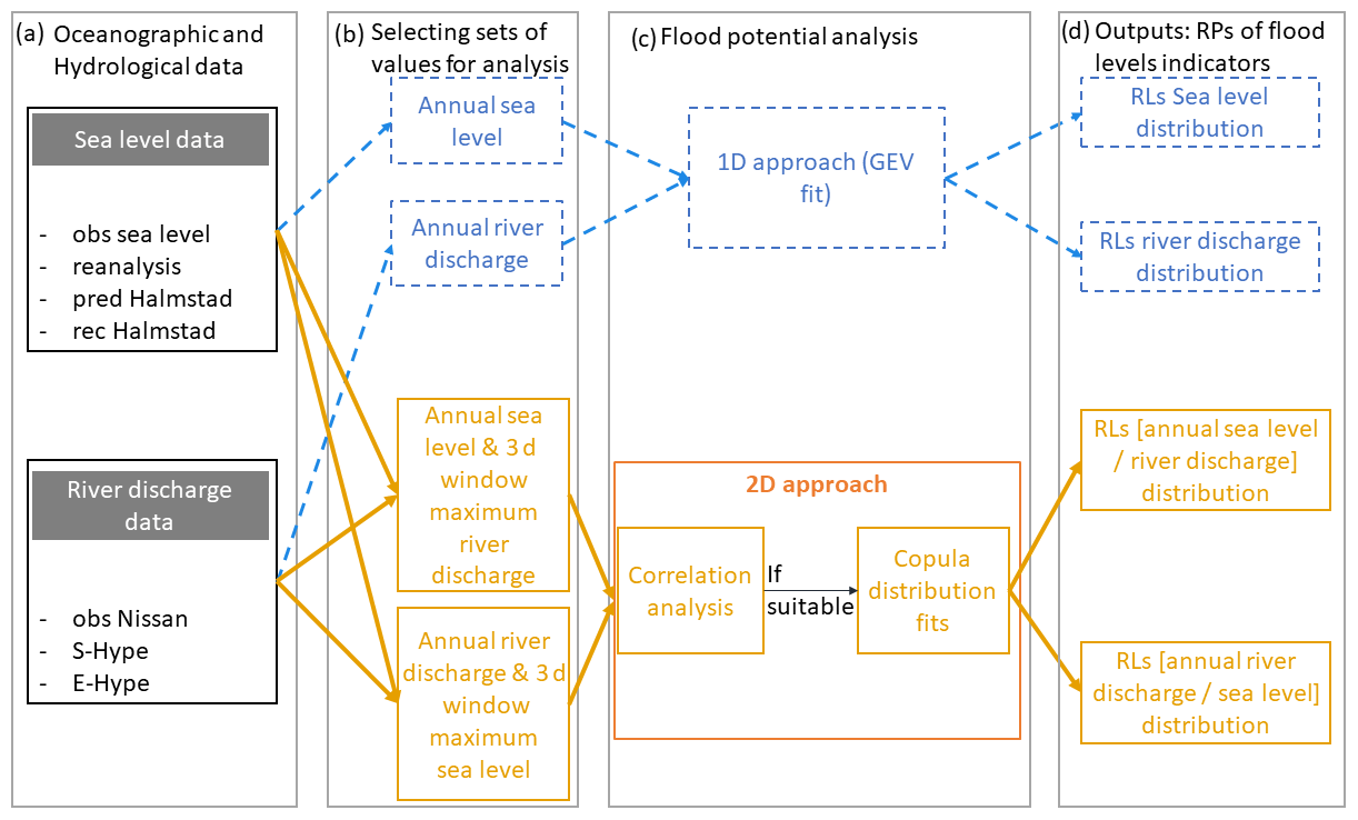
Figure 2 Workflow describing the methodology used in this paper, starting from the oceanographic and hydrological data (a) to the univariate (in blue and dashed arrows) and bivariate (in orange and continuous arrows) approaches used for flood hazard analysis. Panel (b) represents the selection sets; the analysis is then described (c), and the analysis results are shown (d).

Not taking compound flooding effects into account may result in an underestimation of the flood hazards in the coastal zone, including river mouths (Ward et al., 2018). Thus, analysing and understanding these events is of high relevance to coastal communities. In this study, we evaluate the potential impact of extreme hydrological and oceanographic coastal events on the coastal city of Halmstad (Sweden), which is a port and industrial–recreational city at the mouth of the river Nissan. Halmstad is located on the west coast of Sweden (Fig. 1) and has been chosen as it is naturally prone to coastal, fluvial, and pluvial flooding. The area is subject to extratropical cyclones (Hoskins and Hodges, 2002; Dacre et al., 2012), resulting in rather high sea levels by storm surges for the area (Wolski et al., 2014). According to the Swedish Meteorological and Hydrological Institute (SMHI), Halmstad recorded the highest-ever sea level measured in Sweden of 235 cm on the 29 November 2015 during the wind storm Gorm. Halmstad has also been severely impacted by river floods. While Nissan is the main river crossing the city of Halmstad, smaller rivers are also present and can create floods, such as the river Fylleån. Finally, the west coast of Sweden is found to be one of the areas in Sweden expecting the most significant impacts due to SLR during this century (Hieronymus and Kalén, 2020). Thus, nearby studies have stressed the necessity to update coastal protection measures along the Swedish (Hieronymus and Kalén, 2022) and the German Baltic Sea shorelines (Kiesel et al., 2023). To help guide and communicate with the local municipalities about their continued work in protecting coastal areas from flooding, we considered it useful to pick one site in this area as an example to showcase the applied methods and their results.

The main goal of the current study is to investigate the impact of different data sources, methodologies, and representations of compound extremes on estimates of extreme water levels. Our main focus is to evaluate the sensitivity of compound flood hazards from river discharge and sea level to data sources, potential sources of uncertainties. Using Halmstad as an example, we explore the potential influence on flood hazard assessments related to compound effects from river flooding within the coastal area.

2 Data and methods

In the following, compound effects are defined in terms of the co-occurrence probabilities between coastal sea level and river discharge when at least one of the two is subject to an “extreme” value. An event is considered in the extreme range when a studied variable reaches its annual maximum value. The annual maximum values will differ between different years in a range between 84 and 235 cm for sea level and 88 and 271 m³ s⁻¹ for river discharge. The correlation between co-occurring events has been studied as it provides insight into the relationship between each set of two variables. The exceedance probability of getting an extreme river discharge associated with a high sea level and the opposite permits the assessment of the potential compound effects between those two processes, but it does not determine impacts from compound flooding either in terms of estimating water level or computing inundation depths. Hybrid statistical–hydraulic modelling frameworks have been introduced to answer such issues and study compound flood impacts (Jane et al., 2022; Moftakhari et al., 2019; Gori et al., 2020; Olbert et al., 2023).

Figure 2 presents the main steps of the workflow describing the methodology; this is described in the following subsections. Firstly, we analysed different time series records of sea level and river Nissan discharge data from models and observations at Halmstad using extreme value theory and a generalized extreme value (GEV) distribution (Coles, 2001) – hereby referred to as the “univariate approach” – to estimate return levels (RLs) on every driver independently. Secondly, we defined sets of coupled events based on single variables. Thirdly, we analysed the correlation between sea level and river discharge events. If this analysis indicated potential for compound events, we studied the co-dependency between the two variables by fitting a copula distribution function (Sadegh et al., 2018). We finally performed a statistical analysis of the compound events to study the differences between each data source and its associated uncertainties.

2.1 Data

An analysis of time series records of sea level and river discharge at Halmstad was carried out. As mentioned above, a univariate distribution was initially fitted based on the GEV distribution and extreme value theory (Coles, 2001) for each time series collected. The temporal differences in the lengths of each dataset induce substantial differences and associated uncertainties, which dominate in the case of extreme RPs. Consequently, a moderately extreme 30-year RP event was chosen as the maximum value considered. For comparison, we also consider more frequent events with a 5-year RP.

2.1.1 Sea level data

Figure 3 displays the different sea level datasets used (Fig. 3a) and their corresponding univariate extreme value analysis (Fig. 3b).

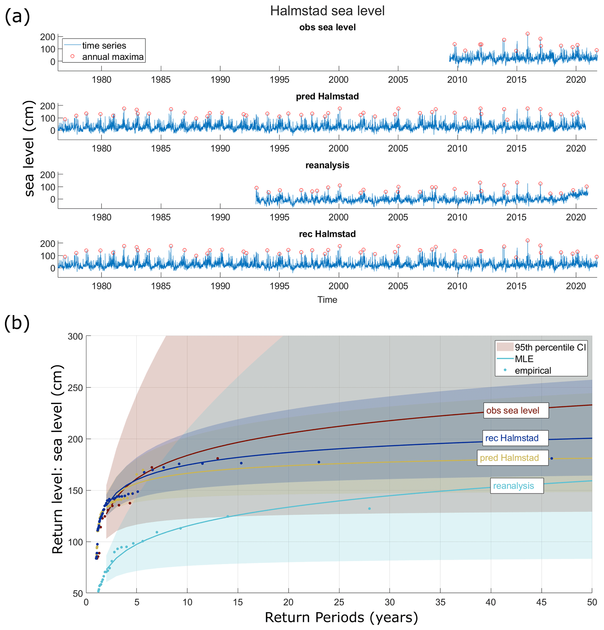
Figure 3 Halmstad sea level time series and annual maxima from different sources: observations (“obs sea level”), reconstructed (“rec Halmstad”), and predicted (“pred Halmstad”), derived from a machine learning model trained on data from the Viken station and reanalysis (“reanalysis”) datasets (a). RLs estimated from corresponding GEV fits of each dataset and the associated 95th percentile confidence intervals (background colours). The dots depict empirical data (b).

Observations

Hourly sea level observation data were obtained from SMHI at Halmstad's tide gauge denoted as the station “HALMSTAD SJÖV” with station number 35115 in the open database provided by SMHI (Fig. 1). This hourly sea level time series is transformed to a daily time series using the maximum hourly data within the day. However, to carry out this analysis, the period with sea level observations (titled “obs sea level”) was insufficient as only a 13-year period (from 2009 to 2021) is available. To extend this sea level record, a set of reanalysis data and a machine learning approach have been investigated and used.

Reanalysis

Hourly sea surface variations (in metres) covering the period from 1993 to 2020 with a spatial resolution of approximately 2 nmi have been provided by the Copernicus Marine Environment Monitoring Service's (CMEMS) Baltic Monitoring and Forecasting Centre (BAL MFC) (CMEMS, 2022). This reanalysis uses the ice–ocean model Nemo-Nordic (Pemberton et al., 2017), and the data are assimilated with the localized singular evolutive interpolated Kalman (LSEIK) method (Nerger et al., 2005). Data are extracted from the closest grid point to Halmstad's tide gauge, and the hourly data were changed to a time series of daily maxima for our purpose to focus on extremes. This sea level dataset is named “reanalysis”.

Machine learning model

A probabilistic machine learning method, random forest (RF), is used (Breiman, 2001). Sea level records from the neighbouring station of Viken (station named “VIKEN”, number 2228 in the SMHI database) are used to train the RF model over an 8-year period, where it is correlated with Halmstad's observed sea level. The resulting sea level estimates at Halmstad include both mean predictions and standard deviation to assess uncertainties and variability following the methodology introduced by Dubois et al. (2024). The last 3 years of available data at Halmstad is used to validate the RF model, emphasizing extreme events predictions. The RF model is used to produce a first dataset called “predicted Halmstad” (“pred Halmstad”) and a second one named “reconstructed Halmstad” (“rec Halmstad”).

The predicted Halmstad dataset provides daily sea level (in centimetres) for the full period of available sea level observations from the station at Viken, here from 1977 to 2021.

The reconstructed Halmstad dataset provides daily sea level (in centimetres). It joins both sets, i.e. combines observations from Halmstad from 2009 to 2021 and the predicted Halmstad data from the RF model from 1977 to 2009. Thus, it also covers the period from 1977 to 2021. Further attempts to enrich the RF model by including reanalysis data (i.e. as part of the training) did not improve the predicted sea levels in the reconstructed datasets significantly, which emphasized the need for local observations. These were fortunately available, even if not for the entire extended period. Similar findings (i.e. significant improvements when using local observations as means to train a machine learning of sea level) were previously found in this region (e.g. Hieronymus et al., 2019).

It is not just the length of the observation period that is short. The reanalysis dataset also exhibits a bias and does not predict the observed extreme sea levels. Accordingly, the uncertainties estimated from both univariate GEV analyses are large (Fig. 3b). The predicted and reconstructed dataset yields result in a smaller uncertainty range. Hence, the reconstructed dataset, which is based on observations when available, was chosen as the best source of sea level information for the bivariate analysis.

2.1.2 River runoff data

Figure 4 presents the different river discharge datasets obtained (Fig. 4a) and their corresponding univariate extreme value analysis (Fig. 4b).

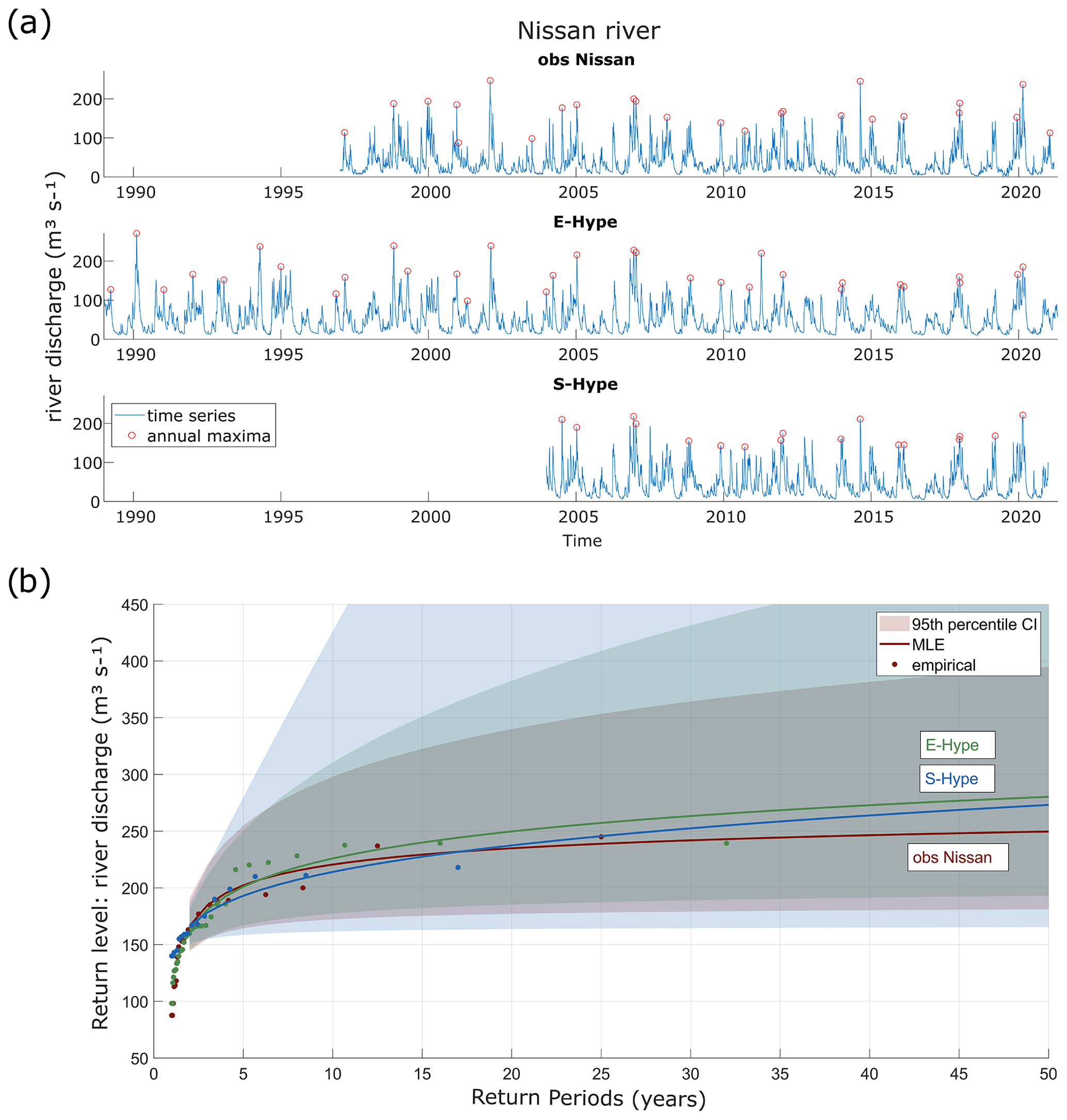
Figure 4 Nissan's river time series and annual maxima from different sources: observations (“obs Nissan”), European HYPE model (“E-Hype”), and Swedish HYPE model (“S-Hype”) from SMHI (a). RLs derived from GEV fits to each dataset are shown with 95th percentile confidence intervals (background colours). The dots are the empirical data (b).

Observations

River discharge data were obtained from SMHI at station 2471: Nissaström (Fig. 1), covering a basin of 2437 km². Observations of daily river discharge in m³ s⁻¹ (obs Nissan) are provided from 1997 to 2021.

E-Hype model

Modelled river discharge data are taken from the Hydrological Predictions for the Environment (HYPE) model, which simulates water flows and quality at different spatial scales (Lindström et al., 2010). A model detailed description can be found at http://hype.smhi.net/wiki/doku.php (last access: 10 September 2023). Daily temperature and precipitation values are used as dynamic forcing in this model. The European HYPE model – E-Hype2016_version_16_g (E-Hype) – provides daily river discharge (in m³ s⁻¹) from 1989 to 2021 (https://vattenwebb.smhi.se/om-vattenwebb, last access: 10 May 2023). The model performs better for annual and seasonal flows compared with daily and extreme flows (Donnelly et al., 2016).

S-Hype model

SMHI has set up the HYPE model for Sweden, now used operationally to forecast hydrological conditions over Sweden, such as floods and droughts. It covers all of Sweden (450 000 km²), where the country has been divided into subbasins of 28 km² on average (Strömqvist et al., 2012). S-Hype3 model's data (S-Hype) of daily river discharge (in m³ s⁻¹) have been provided from 2004 to 2020 (Donnelly et al., 2016). The model seems to slightly underestimate high-flow peaks with high-flow statistics, differing by around ±10 %, whereas the mean flow is highly reliable (Bergstrand et al., 2014).

The available time series associated with the S-Hype model is rather limited, leading to a wide uncertainty band when carrying out the univariate analysis (Fig. 4). Conversely, the Nissan observations and E-Hype datasets lead to RLs that are associated with more bounded uncertainty estimates. In this light, we choose the E-Hype dataset for the bivariate analyses as the data are available over a more extended period. The largest RLs are seen for the E-Hype dataset for RPs above 5 years.

2.1.3 Sets of coupled events

To study compound events in a river mouth environment from both a river discharge and sea level perspective, we defined two different sets of events based on the data discussed above. The first one paired sea level annual maxima (S_n) and associated daily maximum river discharge (q_n) within a defined time period centred on the date of S_n (±Δ days). The second one pairs river discharge annual maxima (Q_n) and associated hourly maximum sea levels (s_n) within a defined 3 d window centred on the date of Q_n (±1 d) (Couasnon et al., 2020; Moftakhari et al., 2017; Sadegh et al., 2018). Each of the four sea level time series observed and modelled records were then correlated with each of the three river discharge ones, which makes up a total of 12 different datasets (Table A2).

2.2 Statistical analysis

Univariate analysis

To estimate the extreme values of Nissan's river runoff and Halmstad sea levels, and their associated RPs, a GEV distribution was fitted to the annual extremes separately for each time series record (Coles, 2001; Ahsanullah, 2016). This was done using the MATLAB-based GEV-fitting algorithm, which provides parameter estimates and 95 % confidence bands. Here, we do not make any assumption concerning the dependence between the two variables of interest, sea level and river discharge; each variable is modelled independently based on its own marginal distribution.

Bivariate analysis

Initially, the Pearson, Spearman, and Kendall correlation coefficients and the associated p values were calculated for each of the 12 collated datasets to assess whether there was a relationship between river runoff and sea level. The usual threshold value of 5 % was defined as evidence for rejecting the H0 null hypothesis; that is, the two variables are independent. When p values were found to be lower than the threshold, the null hypothesis could be rejected, and the two variables were similarly found to show significant dependency. However, when p values are above 5 %, H0 cannot be rejected, so the two variables can be independent.

To represent the compound extremes, we apply copula modelling, which has been found to be useful for representing a joint probability (Hao and Singh, 2016). The analyses were carried out using the Multi-hazard Scenario Analysis Toolbox (MhAST) Version 2.0 from Sadegh et al. (2018). The copula method models the dependence structure of the two random variables (Joe, 2014; Sadegh et al., 2017). It links or joins individual univariate distributions into a joint multivariate distribution that has a specified correlation structure (Tootoonchi et al., 2022). MhAST fits 25 different copulas to an input dataset. It first calculates the best possible fitting marginal distribution for each univariate dataset. It then proposes the best copula fit based on the maximum likelihood, Akaike information criterion (AIC), and the Bayesian information criterion (BIC). The root mean square error (RMSE) and Nash–Sutcliffe efficiency (NSE) values are calculated for each copula. Here, we evaluated the difference between each of the copula fits. A joint RP can then be calculated based on the copula but results in statistically similar infinite combinations of sea level and river discharge values for each RP event (Sadegh et al., 2018). The scenario with the highest density along the closed-form joint probability density function of the copula permits the identification of the most likely scenario. This scenario is based on the copula fit parameters, which represent the statistical relationships between the individual hazard components coming from the input samples. An uncertainty analysis was also carried out using MhAST with a “weighted average” and a “maximum density” approach (Sadegh et al., 2018). This first approach reproduces a distribution of potentially compound hazards. Based on the determined joint probability contours, random samples are weighted from the critical joint RP; 1000 weighted samples are randomly drawn from it. Therefore, a sample with a higher joint probability density value has a higher chance of selection. This approach effectively generates a distribution of potential compound hazards while considering the underlying copula structure. This provides a comprehensive overview of the overall range of possible compound hazards. The second approach is based on the most likely scenario and provides an uncertainty range around it. A range of possible most likely scenarios can be generated based on the different copulas issued from the same copula family that best describes the input datasets, allowing for the quantification of uncertainties around this central scenario (Sadegh et al., 2018).

Two types of hazard scenarios (HSs) have commonly been proposed to study the hazard of compound floods related to sea level and river discharge (Salvadori et al., 2016; Moftakhari et al., 2019; Serinaldi, 2015). The “AND scenario” corresponds to a scenario where both the river discharge and the sea level are large enough to make a bivariate occurrence hazardous, meaning that both high sea levels and river discharge exceed the respective random variables concurrently. The “OR scenario” corresponds to a scenario where either the river discharge or the sea level or both are large enough to make a bivariate occurrence troublesome, meaning that either of the extremes exceeds the respective random variable with a time offset within a limited time interval (Requena et al., 2013).

2.3 Methodology

Firstly, a correlation analysis was carried out for each set, as proposed in Sect. 2.2. This analysis investigated the significance of independence between the sea level and river discharge during extreme occurrences. Then, each set was used as input to MhAST, which performed the compound analysis and returned 25 copula fits ranked depending on different criteria (Sect. 2.2). Among the 25 copulas fitted, only the ones presenting a closed-form joint probability density function (Sadegh et al., 2017) were further investigated since, in these cases,`most likely scenarios and their associated uncertainties can be defined. Chosen RLs were calculated for each copula, and their uncertainties were assessed. Adopting the “AND scenario” (see above) permitted us to investigate the hazard of compound events only, highlighting the dependency between sea level and river discharge during extreme events. Conversely, the “OR scenario” was finally preferred when looking at RLs as this looks into the “total” flood hazard, whether originating from hydrological, coastal sources, or both in combination.

To compare and evaluate the role of copulas and the role played by sea level and river discharge, respectively, a notion of normalized difference value (NDV) was introduced. We defined it as the normalized difference between the RL values of interest from the bivariate analyses. Here, we normalize relative to the corresponding E-Hype univariate RL, which yields a representative dimensionless quantity. It should be pointed out that this quantity does not represent the “amplification” with respect to the univariate case since, as shown by Serinaldi (2015), one cannot compare RLs of different dimensionality. Suppose we investigate the resulting spread from using different copulas (based on the most likely scenarios within one set under the 5-year RP); the NDV is calculated as the difference between the maximum and minimum value of the most likely scenarios for any copula within a specific set divided by univariate 5-year RL derived from the E-Hype dataset (Sect. 3.2). When we look into the sensitivity of river discharge datasets, the sea level dataset is fixed, and the NDV is measured as the normalized difference between the maximum and minimum values of the most likely scenarios of best fits among the three sets of associated river discharge divided by the corresponding E-Hype univariate RL and, vice versa, when looking into the sensitivity of sea level datasets. The NDV term indicates the magnitude of change or difference in RL results we can expect when choosing a certain copula or input dataset. Very small NDVs suggest that the corresponding choice of a variable of interest does not strongly influence the results. In contrast, large NDVs indicate that a particular choice results in significant differences.

3 Results and discussion

From the rank correlation analysis, the datasets based on sea level annual maxima (S_n,q_n) did not reveal any significant dependency (i.e. “compoundness”) between sea level and river discharge; therefore, no copula analysis was done (Table A1). In this case, the univariate analysis seemed to fit best under the proposed conditions of this study. Conversely, the datasets based on river discharge annual maxima (Q_n,s_n) yielded significant dependencies, suggesting a possible compound impact on river discharge. In Sects. 3.1 and 3.3.1, we look into the “AND scenario” as we investigate the compound hazard only. In the Sects. 3.2 and 3.3.2, we mainly focus on the “OR scenario” (see above) as we are interested in the total flood hazard driven regardless of the situation (oceanographic, hydrological, or compound). The set rec Halmstad–E-Hype is chosen as our base case because it has the longest co-occurring period (Table A2).

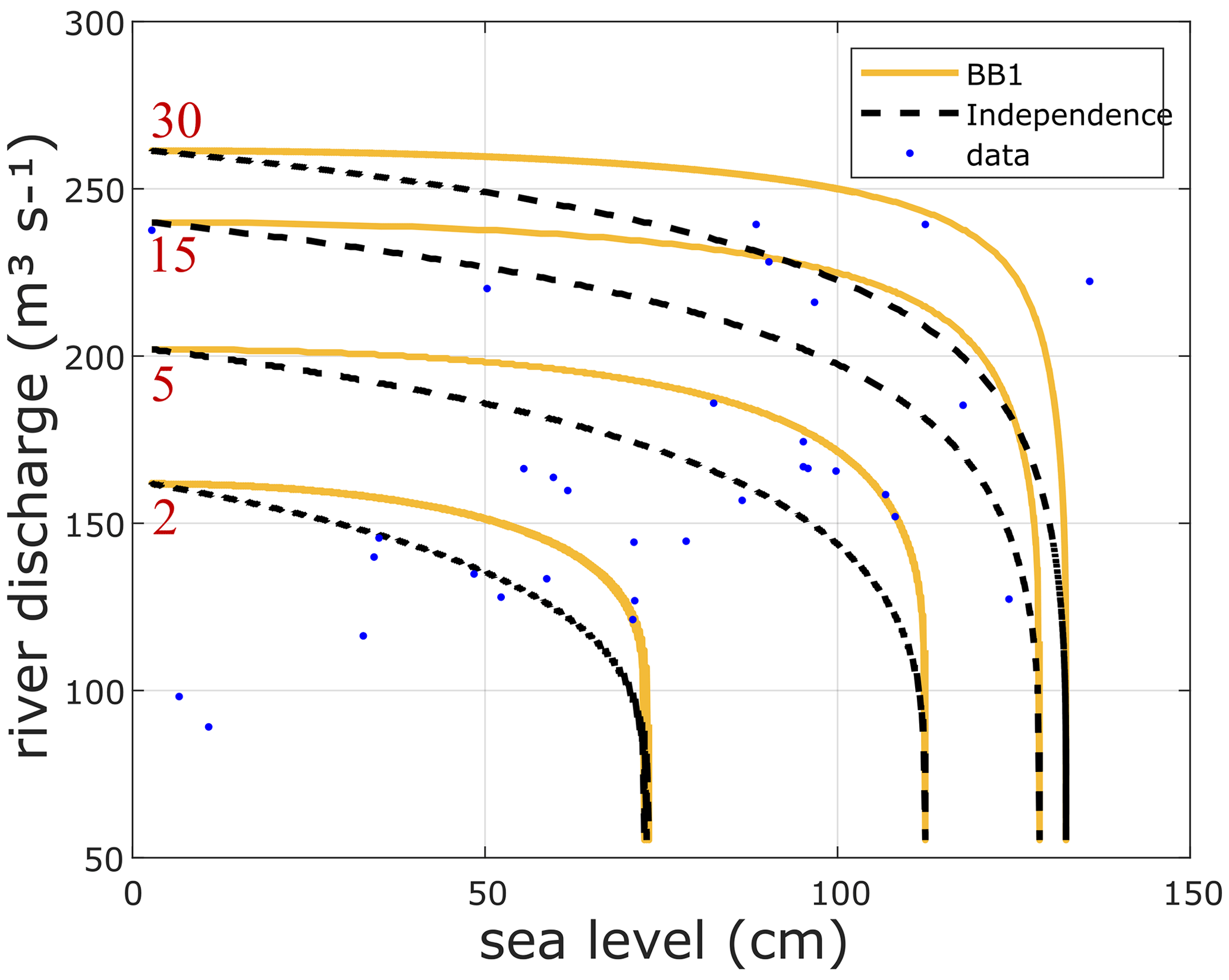
Figure 5 RLs for base case set rec Halmstad–E-Hype. Full lines correspond to the return period (RP) isolines for joint probability (AND scenario) of river discharge (y axis) annual maxima and associated sea level (x axis) maxima (Q_n,s_n). The dashed lines represent the distribution fit, assuming the independence between the variables. Blue dots show observed data. The BB1 copula is used to model the dependence of river discharge annual maxima and associated sea level maxima calculated for each RPs visible in red text (2, 5, 15, and 30 years).

3.1 Dependency/independency of the variables

Figure 5 and Table A1 show the dependency between the river discharge annual maxima and associated sea level local maxima (Q_n,s_n) event sets as expressed in Sect. 2.1. Figure 5 displays the best copula distribution fit: BB1 from the rec rec Halmstad–E-Hype set under the “AND scenario” hypothesis for the 2-, 5-, 15-, and 30-year RPs. The full lines depict the RLs considering sea level and river discharge as dependent variables (derived from the best copula distribution fit). In contrast, the dashed lines show analogous results when assuming the two variables to be independent. The figure shows that the lines do not overlap, highlighting a dependency between both variables. Also, for all RLs presented, each RL from the independent hypothesis (dashed line) is placed below each corresponding RL from the dependent hypothesis (full line), supporting the hypothesis that compound events lead to higher flood risks when considering compound extremes as also found in Bevacqua et al. (2017), where they studied compound hydrological and oceanographic floods in Ravenna (Italy). Therefore, for example, a 30-year RP, when looking at the independent variables, would become a 13-year RP when considering the variables' dependency. This frequency increase comes from the compound effects and can be highlighted for each RP and copulas tested. Also, the dependency between extreme hydrological conditions and high oceanographic ones stresses the presence of compound effects, which lead to higher levels of river discharge and sea level during such events at the estuary. Joint probability contours are derived, which permits obtaining a probability of co-occurrences for a possible event along each curve, which is later used to carry out the uncertainty analysis (Sadegh et al., 2018). For example, along the 5-year RP curve, the probability of getting a 5-year RL of 180 m³ s⁻¹ river discharge and 93 cm sea level is higher than getting one of 201 m³ s⁻¹ and 20 cm or one of 101 m³ s⁻¹ and 112 cm (Fig. A1).

3.2 Compound hazard potential on river floods

The focus is on river discharge RLs as a proxy for fluvial flooding indicators. Figure 6 represents the 5- and 30-year river discharge RLs from the set rec Halmstad–E-Hype under the “OR scenario” hypothesis for each copula tested and its associated uncertainties values from two approaches. The best copula fit selected based on the different criteria as AIC in this case (Sect. 2.2) is BB1 (red diamond). The stars and diamonds represent the maximum density of the calculated RL for each copula, which can be interpreted as the most likely scenario under the bivariate analysis.

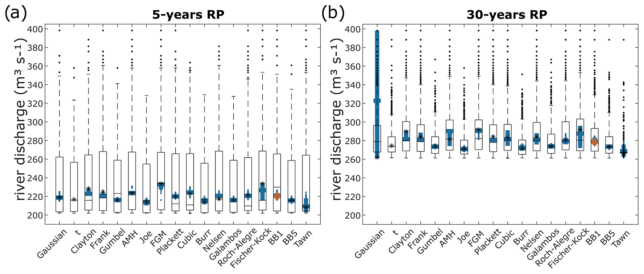
Figure 6 Fluvial component in bivariate events with 5-year (a) and 30-year (b) return periods from copula fits for rec Halmstad–E-Hype. Each column represents a copula distribution fit. Stars represent the most likely scenario return values from each copula for each set, and the red diamond is the best copula fit. Two uncertainty approaches are displayed as boxplots, giving a statistical summary. Median and first and third quartiles are represented in each box, whiskers represent minimum–maximum values, and dots represent outliers. Outlined boxplots correspond to the “weighted average” approach, and filled ones to the “maximum density” approach.

RP = 5 years

The 5-year RL from the E-Hype model is 201 m³ s⁻¹ with a 95th percentile confidence interval of 167–246 m³ s⁻¹ under the univariate GEV distribution fit. The BB1 copula fit has a 5-year RL most likely scenario of 220 m³ s⁻¹. Among all tested copulas, their 5-year RLs of most likely scenarios differ around 26 m³ s⁻¹, all between 208 and 234 m³ s⁻¹. The RL copulas' uncertainties are displayed with the boxplots from two methods: the weighted average approach shown with the outlined error bars and the maximum density approach shown with the filled error bars. The weighted average approach gives larger uncertainty ranges than the maximum density (Sect. 2.2). Indeed, for the best copula fit, the maximum density approach looking at the uncertainty of the most likely scenarios results in a narrow band of a maximum of 19 m³ s⁻¹ per copula against a more extensive range of 159 m³ s⁻¹ going from 202 to 361 m³ s⁻¹ with the weighted average approach. All copulas present a similar pattern.

Moreover, the RL uncertainties for the maximum density approach are all located within the 95th confidence interval of the univariate RL. However, the weighted average approach gives a 75th percentile of around 255 to 269 m³ s⁻¹ and a nonoutlier maximum of around 324 to 361 m³ s⁻¹ above the 246 m³ s⁻¹, corresponding to the 95th percentile of the univariate GEV fit, indicating the importance of considering the bivariate analysis method. The BB1 copula chosen as the best fit here by the different evaluation criteria mentioned in Sect. 2.2 presents neither the smallest nor largest uncertainty band.

RP = 30 years

The 30-year RL from the E-Hype model is 263 m³ s⁻¹ with a 95th percentile confidence interval going from 189 to 431 m³ s⁻¹ under the univariate GEV distribution fit. The BB1 copula fit has a 30-year RL of 278 m³ s⁻¹. The copulas' 30-year RLs of most likely scenarios differ by around 25 m³ s⁻¹, with all of them between 267 and 292 m³ s⁻¹, except for the Gaussian copula. For all copulas except the Gaussian one, the weighted average approach gives a more extensive uncertainty range than the maximum density one. Indeed, for the best copula fit, the maximum density approach results in a relatively narrow band of 24 m³ s⁻¹, going from 272 to 296 m³ s⁻¹, against a more extensive range of 92 m³ s⁻¹ going from 261 to 353 m³ s⁻¹ with the weighted average one. All copulas except the Gaussian and the Tawn ones present a similar pattern. Moreover, all RL uncertainties for both uncertainty analysis approaches are within the 95th confidence interval of the univariate RL for the 30-year RP.

Sensitivity to the choice of copula

For both 5- and 30-year RPs, the copulas and their associated uncertainties present a similar pattern. Depending on the choice of copulas, the most likely scenarios differ up to 26 m³ s⁻¹ for the 5-year RP and up to 25 m³ s⁻¹ for the 30-year RP, with the Tawn copula giving the minimum value and the Fischer–Kock and Farlie–Gumbel–Morgenstern (FGM) copulas giving the maximum value. When only looking at the most likely scenarios values for each copula, they differ in a range approximately equal to 13 % and 9.5 % for the 5- and 30-year RPs, respectively (Table A3). For each copula, the uncertainties' relative errors based on the maximum density approach differ from 1 % (Gaussian) to 9.9 % (Fischer–Kock) and from 2.3 % (Joe) to 52 % (Gaussian) for the 5- and 30-year RPs, respectively, and from 63 % (Joe) to 75 % (Fischer–Kock) and from 16 % (Joe) to 35 % (Fischer–Kock) for the weighted average approach. For comparison, the relative errors for the univariate GEV fit are around 41 % and 92 % for the 5- and 30-year RPs, respectively. When considering the maximum density uncertainties, all RLs of all copula are in the range of 208–234 m³ s⁻¹ for the 5-year RL and 262–398 m³ s⁻¹ for the 30-year RL (Table A3; Fig. 6).

These differences in resulting RLs emphasize the importance of the role played by the choice of copulas and the consideration of quantifying uncertainties.

3.3 Sensitivity analysis on compound flood hazard potential: OR scenario

This section focuses on the impact of data sources on resulting RP statistics, aiming to compare copula analyses considering compound events. As seen in Sect. 2.1, we have 12 possible datasets to analyse for Halmstad city extracted from models and observations. As mentioned in Sect. 2.1, the univariate analysis presents different results, including RL values and confidence intervals for each river runoff time series.

The 5-year and 30-year univariate RLs of river runoff, respectively, differ by around 9 and 21 m³ s⁻¹ with values of 202 and 241 m³ s⁻¹ based on an observation gauge (red), 193 and 252 m³ s⁻¹ based on the S-Hype model (blue), and 201 and 263 m³ s⁻¹ based on the E-Hype model (green) as displayed in Fig. 4b. However, uncertainties associated with the 95th percentile confidence interval differ vastly from, respectively, around 86 and 185 m³ s⁻¹ (observation), 121 and 811 m³ s⁻¹ (S-Hype), and 79 and 242 m³ s⁻¹ (E-Hype) as displayed by the background colours on the figure.

3.3.1 Dependency/independency of the variables

Figure 7 presents resulting RLs for combined ranges of each variable set for the 5- and 30-year RPs as in Fig. 5 but with results from six different data sources to study the resulting impacts. The dependency is evident for each set, with each full line moved away from its corresponding dashed line, highlighting the dependency and compound effects for any sets tested. The differences between solid and dashed lines in Fig. 7 are typically contained within about 20 cm sea level or 25 m³ s⁻¹ river discharge based on the maximum distance between the copula and independence cases on rays coming from the origin, constituting about 10 %–15 % of the extreme 5- and 30-year RLs for the site with a gap increasing with higher RPs. At first glance, these differences may be perceived as a reasonably small compound effect, but every little increase in extreme situations can have a consequence for society. It should be noted that switching data sources may have a significant effect on estimated RLs; hence, both method and choice of data are essential.

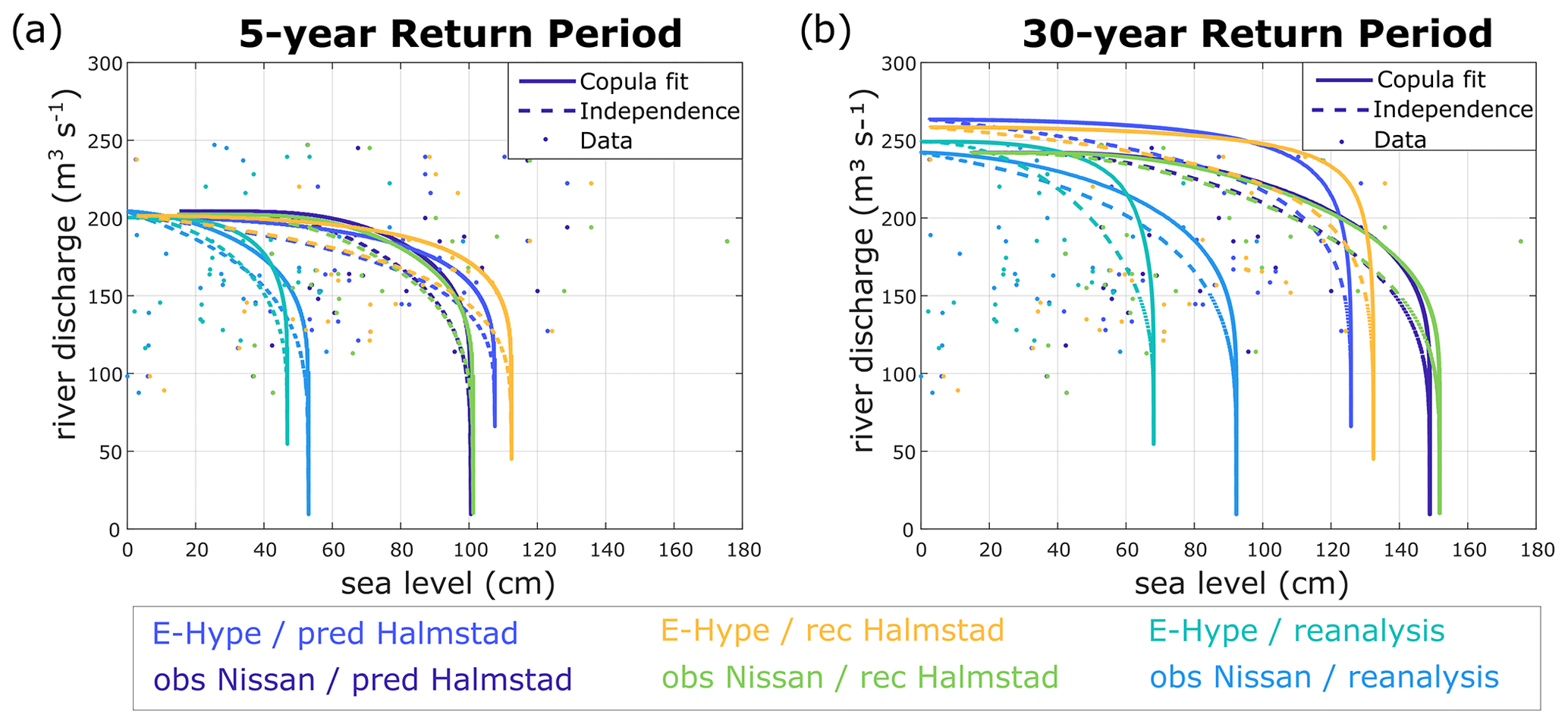
Figure 7 The 5-year (a) and 30-year (b) return period isolines for joint probability (AND scenario) of river discharge (y axis) annual maxima and associated sea level (x axis) maxima (Q_n,s_n) for Halmstad. Full lines implement the compound effect, and dashed lines represent fit, assuming independence between both variables. Dots show observed data. The best copula fit is used to model the dependence of Q_n,s_n calculated for each set visible in coloured text.

Some sets behave similarly, as their corresponding dashed and full lines almost overlap, for instance obs Nissan–pred Halmstad with obs Nissan–rec Halmstad or E-Hype–pred Halmstad with E-Hype–rec Halmstad in both 5- and 30-year RPs (Fig. 7). This similarity emphasizes that river discharge dominates the co-occurrence probabilities of bivariate hazardous events over sea level inputs.

3.3.2 Compound hazard potential on river floods

The most likely scenarios of 5- and 30-year RPs and their associated uncertainties on the different sets are calculated as described in Sect. 2.1. This study focuses on extreme hydrological events associated with oceanographic conditions and, therefore, concentrates on the RLs of river discharge. Figures A2 and A3 display those results for each set in the same way as Fig. 6: Fig. A2 the results of the 5-year RP and Fig. A3 those of the 30-year RP analysis.

Under the 5-year RP, lower RLs are found for all obs sea level sets (Fig. A2), corresponding to the data available and short duration of overlapping periods, with a maximum of 13 years and limited by the extent of sea level observations. Under the 30-year RP, lower RLs are found for the set E-Hype–obs sea level and all S-Hype sets except for S-Hype–obs sea level, which presents the most extreme values (Fig. A3).

For the 5- and 30-year RPs, the three sets associated with the E-Hype model, which show statistical significance, lead to similar and higher values, respectively, than all the other sets. The last set showing statistical significance is associated with the S-Hype model and leads to somewhat different results between the 5-year RP, with slightly lower RLs, and the 30-year RP, with generally higher RLs (Figs. A2 and A3). It stresses that the dependence changes the RP results, as also shown by Santos et al. (2021), who studied compound surge and precipitation events in a case study in the Netherlands.

All most likely scenario values calculated from the copula analysis under both the 5- and 30-year RPs are within the range of the 95th percentile confidence interval of the univariate GEV distribution fit (Figs. A2 and A3).

Uncertainties associated with the copula analysis and following the maximum density approach do not extend too much from the median values and stay within the confidence interval of the univariate GEV distribution (Figs. A2 and A3) for most of the copulas tested. Under this maximum density approach and based on the best copula fits, they differ by about 3–8 m³ s⁻¹ for the 5-year RP and 2–9 m³ s⁻¹ for the 30-year RP. Under those same conditions, the uncertainties from the weighted average approach vary between 65 and 149 m³ s⁻¹ for the 5-year RP and between 37 and 68 m³ s⁻¹ for the 30-year RP. Therefore, uncertainties related to the maximum density approach associated with the most likely scenarios are relatively small, providing reasonable confidence in such scenarios. Conversely, the weighted average approach uncertainties provide a confidence interval on possibly more extreme scenarios, which is relevant when communicating RLs.

Input dataset selection

Depending on the choice of river time series as initial input, the results of the copula analysis under the 5- and 30-year RPs differ substantially around a maximum of 20 and 40 m³ s⁻¹, respectively, with an NDV range of 6 %–10 % and 8.4 %–15 % (Fig. 8). This contrasts with the choice of sea level time series as initial input with a maximum difference of around 6 and 12 m³ s⁻¹, equivalent to 1.5 %–3 % and 2.3 %–4.6 % NDV bounds for the 5- and 30-year RPs, respectively, without considering the three sets associated with obs sea level. Those results are based on the most likely scenarios from each best copula fit and did not consider the sets associated with obs sea level. It emphasizes that the choice of sea level records has a lower influence than the one of river discharge within this study on compound hydrological extreme events on our example study site (Halmstad). The well-recognized issues from the reanalysis dataset support this result as even a large difference in the sea level input dataset does not get reflected in the NDV values when looking at the choice of sea level. Similar findings could be expected for the surrounding area (west coast of Sweden).

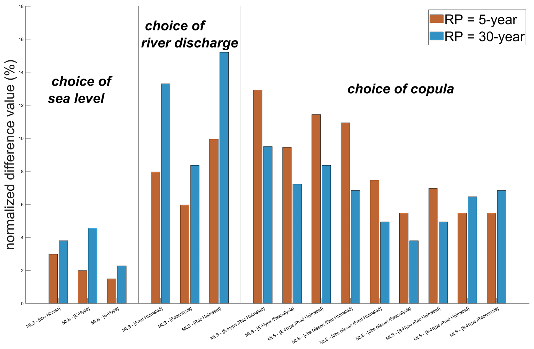
Figure 8 Normalized difference values (%) for evaluating the importance of copula fit and forcing data for both 5- and 30-year return periods, as mentioned in Sect. 3.3.2.

Copula selection

To evaluate the role played by choice of the copula, we calculated the NDV for each set between the maximum and the minimum values returned by the 18 copulas tested without considering the sets with obs sea level data input as it was too short for bivariate analysis. Among all the different sets, the BB1, the Gaussian, and the Clayton copulas are the best ones based on the different statistical criteria (Sect. 2.2). Moreover, when only looking at the sets associated with the same river runoff input, the best copula fit is the same: Clayton for obs Nissan, BB1 for E-Hype except for S-Hype, which has Gaussian as the best fit for S-Hype–rec Halmstad, and Clayton for the two other sets. The tests of using multiple copulas have also been investigated in previous studies. Lucey and Gallien (2022) looked at compound coastal events linking precipitation and/or sea level in a tidal and semiarid area. They noticed that, in their particular area, the Nelsen, BB1, BB5, and Roch–Alegre copulas represented their datasets best, and each of them provided similar results in almost all cases. Bai et al. (2020) introduced a mixed copula, which is a linear combination of Gumbel, Clayton, and Frank copulas, to statistically study coastal winds and waves. They observed that the mixed copula can better describe the dependency structure than the five single copulas tested (Gaussian, t, Gumbel, Clayton, Frank), where the representation of relations between both drivers is complex.

For most of the sets, the “Fischer–Kock” and the “FGM” copulas give the highest RLs, and the “Tawn” and “Joe” copulas give the smallest ones (Figs. A2 and A3). It results in NDVs between 5.5 % and 13 % for the 5-year RP and between 3.8 % and 9.5 % for the 30-year RP. The base case E-Hype–rec Halmstad presents the highest NDVs compared to other sets NDVs, which emphasizes that the choice of copula is relatively more important than in other sets (Fig. 8). Based on our assumption that this is possibly the best set, in terms of data sources, it stresses the idea that the choice of copula becomes more and more critical when input datasets are long enough and statistically significant.

Therefore, the choice of copula has a similar influence to the choice of river discharge records for each of the nine sets tested here, as the obs sea level has not been considered. For both the 5- and 30-year RPs, the choice of sea level is the least impactful. Under the 5-year RP, the choice of copula is overall the most important before the choice of river discharge, but under the 30-year RP, the choice of river discharge predominates. However, this differs when looking at specific sets' copula NDVs (Fig. 8).

4 Limitations

Observed time series datasets have a relatively short length, leading to rather high uncertainties once the GEV analysis is applied. Similarly, model time series datasets have inherent uncertainties, which can be challenging to quantify. Various data sources were assessed for their applicability in bivariate analysis, and direct sea level observations available for only 13 years were a limiting factor. We focus on longer reconstructed time series and other data sources for the principal analysis to explore uncertainties which are linked with available datasets of different lengths and biases. For example, reanalysis-driven storm surge and different modelling approaches such as S-Hype and E-Hype models present some uncertainties due to the modelling nature of such datasets, especially with regards to the extremes, where they are often underestimated. Moreover, assumed stationarity within the datasets can be a limitation while performing the statistical analysis (Kudryavtseva et al., 2021) even though for the neighbour station of Ringhals it has been shown that nonstationary models were not statistically significant (Rydén, 2024). The choice of the sampling datasets based on annual maxima can be a limitation. For instance, in their specific tide-dominated and semiarid area, Lucey and Gallien (2022) stated that annual maximum sampling seems to underestimate water levels at longer RPs. In this study, only the compounding between sea level and river discharge has been studied, but Latif and Simonovic (2023) showed that considering the three drivers storm surge, precipitation, and river discharge to study compound coastal floods can provide a better statistical approach and therefore better estimate joint RPs in their study area located on the west coast of Canada. However, after carrying out a brief sensitivity analysis on defining extreme sea level events as sea level peaks above the 95th or 99th percentile and comparing it with the annual maxima sampling, no noticeable changes were found; a similar conclusion was also drawn by Ward et al. (2018).

A compound analysis is seen as a relatively new approach within this field of study, which also involves some limitations, such as the quantification of uncertainties within a multivariate analysis that differ widely depending on the choice of copula. The uncertainty resulting from the choice of copula can to some extent be constrained by adopting appropriate goodness-of-fit statistics for the selection of the best-fitting copula. In this study, we choose to illustrate this indirectly by presenting results from many different choices of copula, despite having calculated such goodness-of-fit metrics (Sect. 2.2). Furthermore, we showed the normalized difference values for different data sources. As discussed in Sect. 2.3 and Serinaldi (2015), a careful interpretation comparing return levels from different hazard scenarios is, however, always needed. In decision-making adapting a strategy such as ours (to include results from all studied copulas and also different data sources) has some limitations in the sense that too much information can sometimes cause more confusion than help the decision. Often it may be possible to argue against some choices of copulas (e.g. the Gaussian copula when the distributions are skewed), and the strategy of constraining the results to one copula or a set of “best-fitting” copulas using some threshold on the goodness-of-fit metrics may be appropriate. For the purpose of our study and the conclusion drawn, we consider, however, that presenting the results from multiple choices of data and multiple copulas is appropriate.

5 Summary and conclusions

This study assesses the hydrological and oceanographic processes that may lead to compound flood effects in Halmstad. The method is easily transferable to other regions or sites. In the paper, we stress the importance of the choice of data sources and copulas for multivariate analysis. Based on our analysis, we conclude the following:

• A dependency is found between the annual maxima of river discharge and the corresponding sea level. The dependency on annual sea level maxima and associated river discharge was not considered significant at this site.

• All values of the most likely scenarios and their uncertainties resulting from the copula analysis are within the range of the 95th percentile confidence interval of the univariate GEV distribution fit.

• The choice of river time series as initial input influences the results of the copula analysis to a higher degree than the choice of sea level time series as initial input.

• Copula choice has a similar influence on return period statistics to the river discharge input for most of the 12 sets tried.

• According to statistical criteria, the Clayton, BB1, and Gaussian (once) copulas performed the best in this study.

Uncertainties in compound flood hazard quantification are essential to consider. They can come from different sources, such as methodology and data sources. Each type of uncertainty from the individual components due to the length of the time series and the modelling ones is also propagated in multivariate risk estimation. This study highlights the need for careful data source selection, as it may give quite different outputs if only looking at one data source, which inherently is associated with some uncertainties. Therefore, this study stresses the importance of the choice of data sources and of copula.

Appendix A

Table A1 Rank correlation (ρ) and p values of the 12 different sets based on $Q_n/s_n$ in columns “/river” and $q_n/S_n$ in columns “/sea”. The best set of study is displayed in bold; p values above 5 % are highlighted in italic.

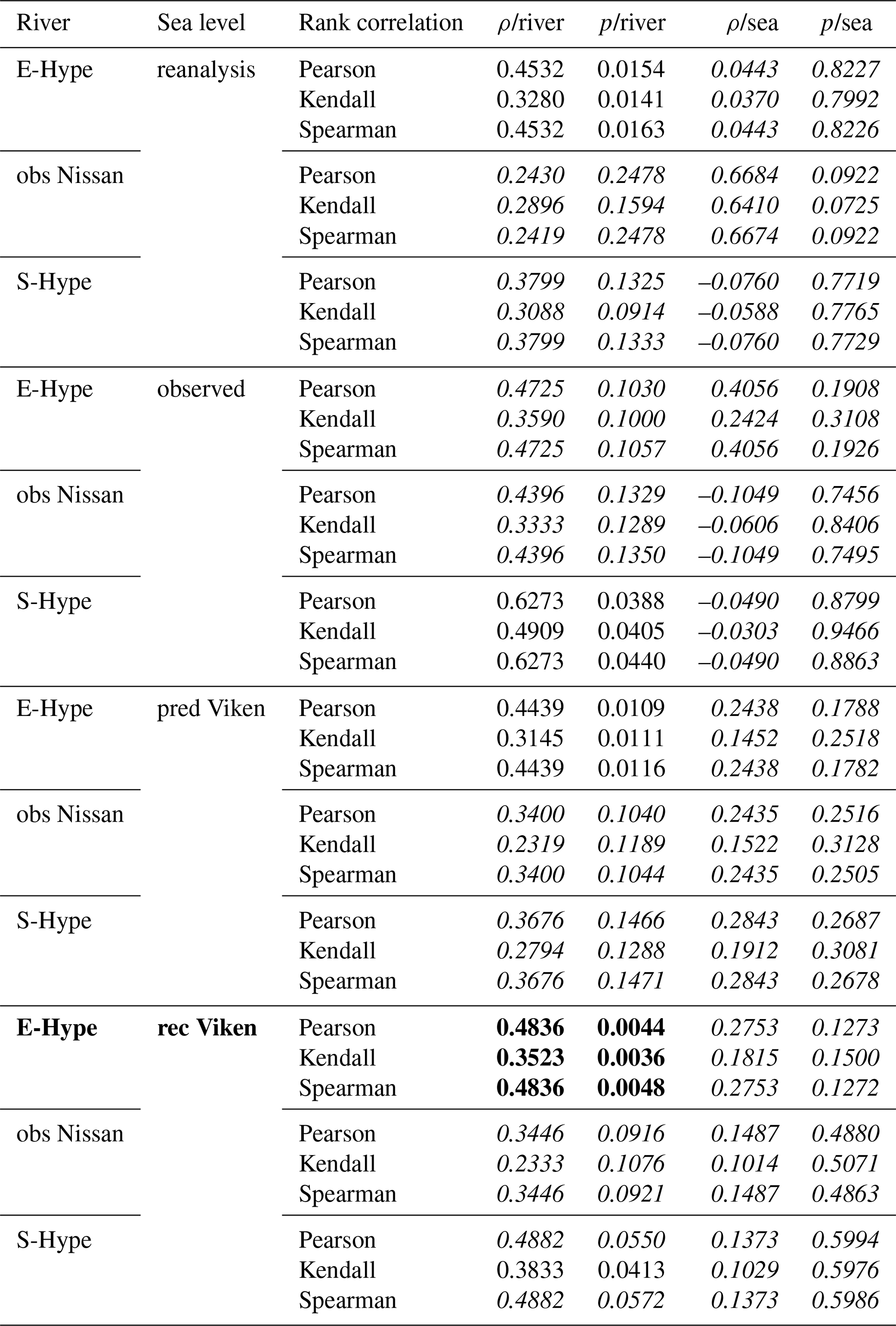
Table A2 Summary report of runs from the copula analysis for the 12 different sets; the best study set is highlighted in bold.

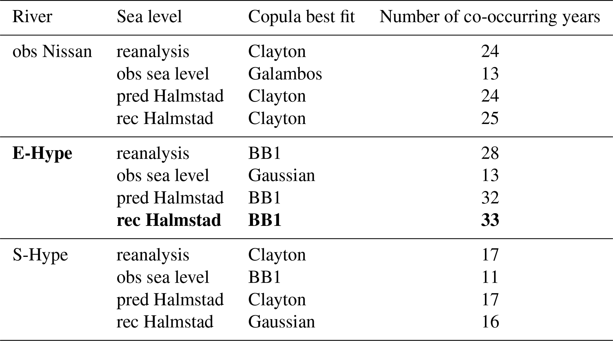
Table A3 Summary report from the river discharge's results and associated uncertainties from the copula analysis for the E-Hype–rec Halmstad set; the results from the univariate method are highlighted in bold. The Gaussian copula has not been considered for the analysis of the most likely scenarios row.

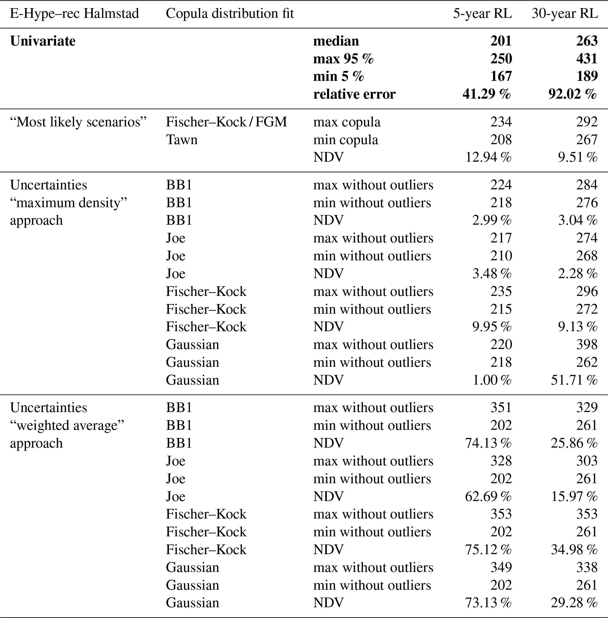
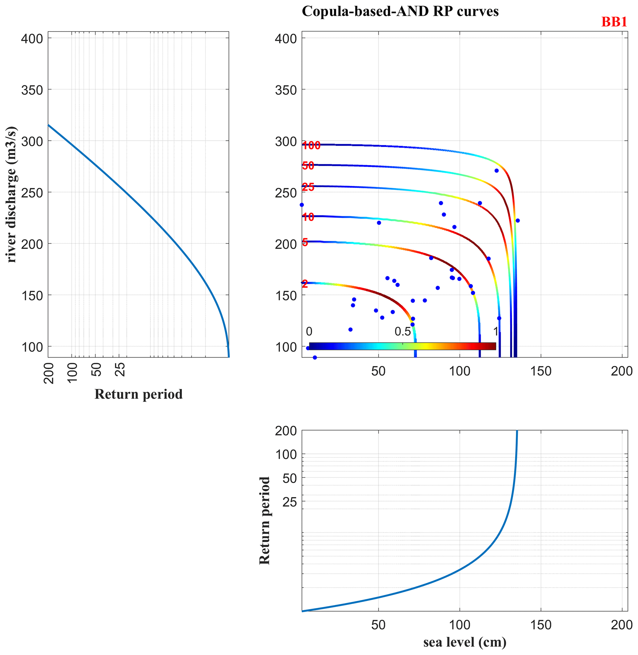
Figure A1 Set E-Hype–rec Halmstad, best copula fit is BB1 displayed with the 2-year, 5-year, 10-year, 25-year, 50-year, and 100-year RPs and associated densities. The left panel and lower panel correspond to marginal RPs curves of each univariate parameter individually, river discharge, and sea level (extracted from MhAST software).

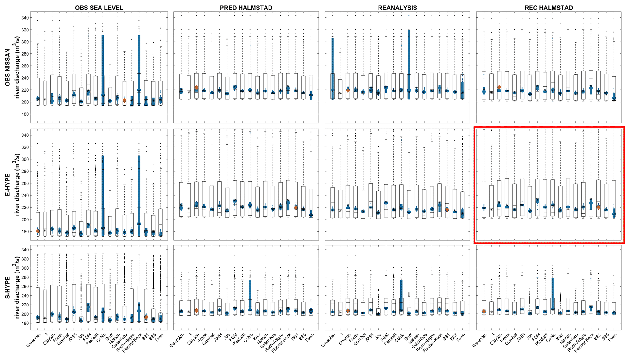
Figure A2 Fluvial component in bivariate events with 5-year RP values from copula fits. Each subplot corresponds to a set of events from an association of river discharge and sea level inputs displayed as a matrix and, in each column, a copula distribution fit where two uncertainty approaches are displayed as error bars. Stars represent the most likely scenarios return values from each copula for each set, and each red diamond is the best-fit copula. The two uncertainty approaches are displayed as boxplots that give a statistical summary. The median and first and third quartiles are represented in each box. Whiskers represent minimum and maximum values, and dots represent outliers. Outlined boxplots correspond to the “weighted average” approach and filled ones to the “maximum density” approach. The set E-Hype–rec Halmstad, used as a base case, is highlighted by the red rectangles.

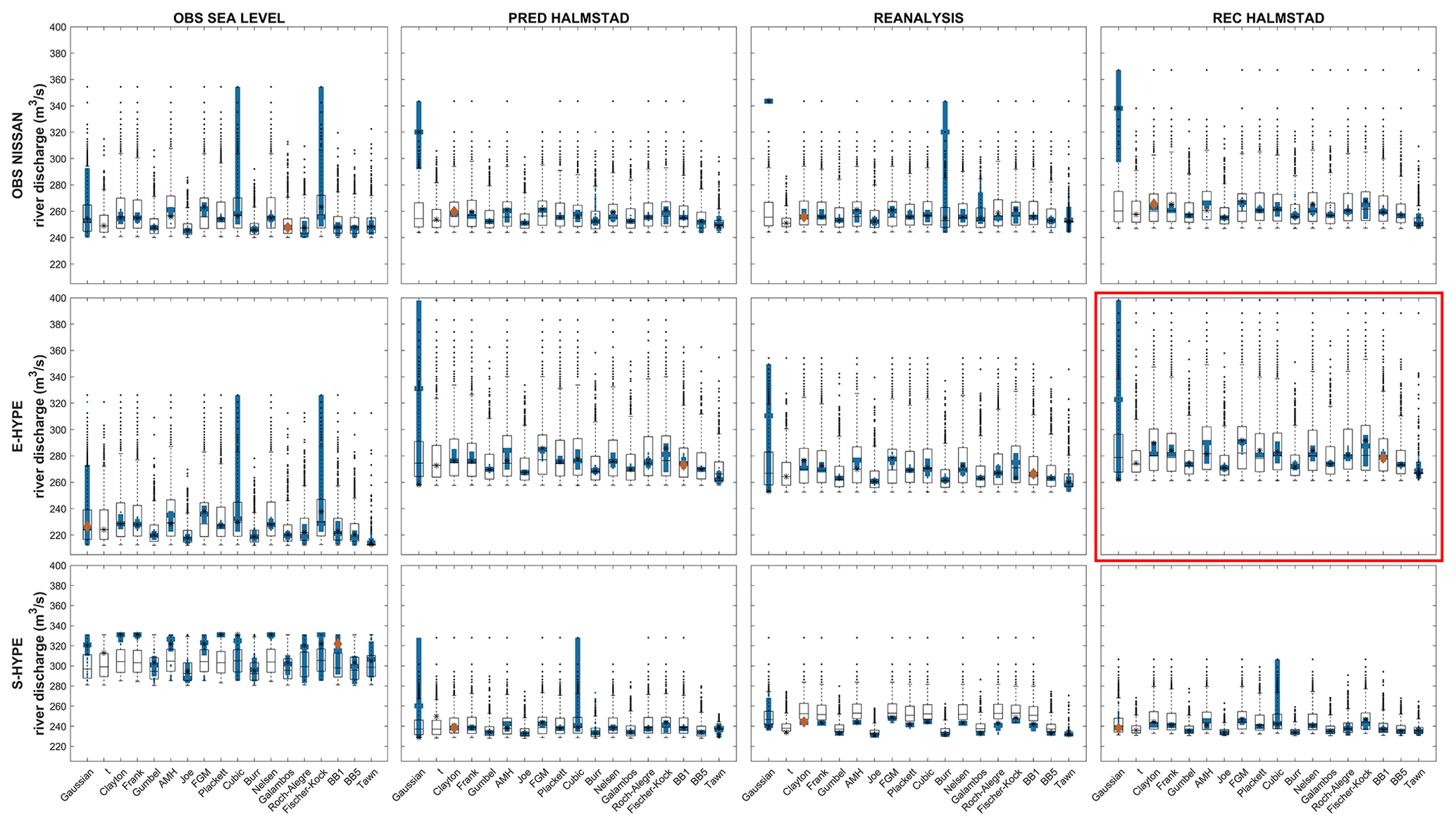
Figure A3 Fluvial component in bivariate events with 30-year RP values from copula fits. Each subplot corresponds to a set of events from an association of river discharge and sea level inputs displayed as a matrix and, in each column, a copula distribution fit where two uncertainty approaches are displayed as error bars. Stars represent the most likely scenarios return values from each copula for each set, and each red diamond is the best-fit copula. The two uncertainty approaches are displayed as boxplots that give a statistical summary. The median and first and third quartiles are represented in each box. Whiskers represent minimum and maximum values, and dots represent outliers. Outlined boxplots correspond to the “weighted average” approach and filled ones to the “maximum density” approach. The set E-Hype–rec Halmstad, used as a base case, is highlighted by the red rectangles.