the Creative Commons Attribution 4.0 License.
the Creative Commons Attribution 4.0 License.
 | 22 Aug 2024
Probabilistic short-range forecasts of high-precipitation events: optimal decision thresholds and predictability limits
François Bouttier
Hugo Marchal
Translation of ensemble predictions into high-precipitation warnings is assessed using user-oriented metrics. Short-range probabilistic forecasts are derived from an operational ensemble prediction system using neighbourhood postprocessing and conversion into categorical predictions by decision threshold optimization. Forecast skill is modelled for two different types of users. We investigate the balance between false alarms and missed events and the implications of the scales at which forecast information is communicated. We propose an ensemble-based deterministic forecasting procedure that can be optimized with respect to spatial scale and a frequency ratio between false alarms and missed events.
Results show that ensemble predictions objectively outperform the corresponding deterministic control forecasts at low precipitation intensities when an optimal probability threshold is used. The optimal threshold depends on the choice of forecast performance metric, and the superiority of the ensemble prediction over the deterministic control is more apparent at higher precipitation intensities. Thresholds estimated from a short forecast archive are robust with respect to forecast range and season and can be extrapolated for extreme values to estimate severe-weather guidance.
Numerical weather forecast value is found to be limited: the highest usable precipitation intensities have return periods of a few years only, with resolution limited to several tens of kilometres. Implied precipitation warnings fall short of common skill requirements for high-impact weather, confirming the importance of human expertise, nowcasting information, and the potential of machine learning approaches.
The verification methodology presented here provides a benchmark for high-precipitation forecasts, based on metrics that are relatively easy to compute and explain to non-experts.
- Article
(8955 KB) - Full-text XML
- BibTeX
- EndNote


Numerical weather prediction increasingly relies on ensemble prediction systems that estimate probabilities of atmospheric events. Ensemble members are computed by numerical integrations of numerical models in order to inform the interpretation of model output in the presence of predictive uncertainties. An important application is the issuance of high-precipitation warnings, which can be useful for protection against flooding and inundation events causing the loss of human life and economic and environmental damage (WMO, 2021).
This work presents a general method for computing high-precipitation forecasts and for measuring their skill. It is tested with a state-of-the-art ensemble numerical prediction system. The dataset used here is relevant for short-range forecasts (for the next few hours) over western Europe. We aim to clarify the conditions under which threshold exceedance for accumulated precipitation can be skilfully predicted as an input to severe-weather warnings. Previous studies have demonstrated that probabilistic forecasts derived from ensembles contain potentially valuable predictive information, but using this information in practical applications is often hampered by challenges in communicating and interpreting probabilities (Joslyn and Savelli, 2010; Fundel et al., 2019; Demuth et al., 2020) This problem is acute for predicting flash floods and inundations because precipitation uncertainties can impact hydrological forecasts, either as drivers of rainfall–runoff models or when they are directly used to estimate flood risks (Cloke and Pappenberger, 2009; Ramos et al., 2010; Hapuarachchi et al., 2011; Zanchetta and Coulibaly, 2020).
Limits to the usefulness of ensemble prediction were explored by Buizza and Leutbecher (2015), who defined the forecast horizon as the range at which the CRPS (continuous ranked probability score) of the ECMWF ensemble system ceases to be statistically better than climatology. In terms of upper-level atmospheric variables, they found that the horizon is several weeks long and depends on the considered horizontal scales, which were on the order of 100–1000 km in their work. Their approach seems difficult to apply to short-range predictions of severe, high-impact weather events that tend to have much smaller scales. Another issue is that the practical significance of skill measures such as the CRPS can be hard to understand for non-expert users.
Here, we focus on high-precipitation events that are conducive to flash floods and on the ability of numerical weather prediction to forecast them with enough anticipation and precision to be useful for issuing severe-weather warnings. Many case studies have demonstrated that current numerical prediction tools have limited skill in predicting high precipitation and flash floods; a common problem is a lack of precision of numerical forecasts of precipitation, as illustrated in articles by Golding et al. (2005); Vié et al. (2012); Davolio et al. (2013); Zhang (2018); Martinaitis et al. (2020); Sayama et al. (2020); Caumont et al. (2021); Furnari et al. (2020); Amengual et al. (2021); and Godet et al. (2023), among others. Precipitation forecast uncertainties are not the only source of errors in flash flood prediction, but they are widely regarded as a major issue that has motivated the development of hydrometeorological ensemble prediction systems. The hope that a detailed representation of precipitation forecast uncertainties will improve estimates of flash flood and inundation risks has been discussed by Collier (2007); Cloke and Pappenberger (2009); Dietrich et al. (2009); Demeritt et al. (2010); Hapuarachchi et al. (2011); Zappa et al. (2011); Addor et al. (2011); Alfieri et al. (2012); and Demargne et al. (2014). Now that high-resolution atmospheric and hydrological ensemble prediction systems are running operationally in several centres, it is interesting to check the relevance of precipitation forecasts in terms of user-specific needs.
Modern regional atmospheric ensemble prediction systems have the appropriate grid resolution and timeliness to simulate high-precipitation events. They use convection-permitting numerical atmospheric models at kilometric resolutions. Several studies have shown that they have skill in predicting localized intense phenomena such as thunderstorms, tornadoes, and high precipitation when compared to lower-resolution model systems (e.g. Stensrud et al., 2013; Clark et al., 2016; Zhang, 2018). Published verification studies of convection-permitting ensembles, however, tend to rely on a few case studies or on precipitation scores at limited intensities.
Here, we aim to quantify the objective value of ensemble-based forecasts of intense precipitation for users interested in categorical yes/no forecasts of future precipitation exceeding predefined intensity thresholds. The originality of this study is that (a) we score short-range precipitation forecasts with the highest-possible intensity given a training dataset of 1 year of ensemble predictions, (b) we focus on performance measures that are most likely to be relevant to forecast end users, and (c) we present an approach that can be applied to generate useful end-user products from ensemble predictions.
The existing literature suggests that these objectives require dealing with three problems: defining scores that are both meaningful to non-experts and appropriate for rare events, designing an effective neighbourhood verification framework to deal with the “double penalty” issue as explained below, and achieving a meaningful balance between event detection and false-alarm rates in the forecast products. Solutions will be presented and discussed in the following.
A key issue is the inherent rarity of high-impact precipitation, which makes it difficult to produce statistical evidence for the value of intense-precipitation forecasts. Verification of probabilistic predictions is tricky for rare events because the low climatological frequency (or base rate) of the events implies that several commonly used scores, such as the area under the relative operating characteristic (ROC) curve or the critical success indicator (CSI), exhibit an excessive sensitivity to hit rates at the expense of false alarms. This problem was recognized as early as Doswell et al. (1990). Attempts to solve this issue (Sharpe et al., 2018; Yussouf and Knopfmeier, 2019) relied on the definition of more appropriate scores, such as the weighted CRPS, the fractions skill score (FSS), and the Symmetric Extremal Dependence Index (SEDI; Ferro and Stephenson, 2011). These scores have attractive theoretical properties such as “being proper”, which make them useful for developers of operational forecast systems because they allow clean comparisons between different systems. Unfortunately they can be difficult to compute and difficult to understand for non-experts, particularly in terms of absolute predictive performance. We argue that, for end users to effectively use ensemble and probabilistic forecasts products, they should have access to clearly understandable performance statistics, as advocated by e.g. Joslyn and Savelli (2010); Ramos et al. (2010); Fundel et al. (2019); and Demuth et al. (2020). We will focus on two scores that are easily interpreted using concepts of detection or false-alarm rates: the equitable threat score (ETS), which is well known in the weather forecasting community (Jolliffe and Stephenson, 2011), and the F2 score, which is standard in the machine learning community (Chinchor, 1992) and has desirable properties with respect to rare events, as explained later.
Another issue is the sensitivity of precipitation scores to the space scales and timescales at which products are used. Ideally, one should focus on scales that are meaningful to the end users. The location and timing errors in extreme precipitation events tend to be similar to if not larger than the size and duration of the events themselves. Thus, grid-scale performance measures of convection-permitting models (at ≈ 1 km scale) will indicate that numerical forecasts have no predictive skill if there is no overlap between forecasts and observed events, a problem called the double penalty effect. To circumvent it, performance measures can be applied to forecasts that have been upscaled by neighbourhood postprocessing in order to assess their skill at resolutions coarser than 1 km. In our study, we will focus on prediction scales on the order of 30 km, which is the typical resolution at which weather warnings are often issued in European countries (Legg and Mylne, 2004). We shall demonstrate that this resolution also makes sense because it is close to the smallest scales at which current numerical precipitation forecasts have significant skill. The design and implications of ensemble neighbourhood postprocessing have been extensively discussed in Ben Bouallègue and Theis (2014) and Schwartz and Sobash (2017). We will use one of their techniques (neighbourhood maximum ensemble postprocessing, or NMEP) in this work because it is relevant to a common objective of high-precipitation warnings: forecasting whether precipitation is likely to exceed a given threshold anywhere within a neighbourhood.
A third issue is the balance between forecast misses and false alarms. Most traditional scores for binary events give similar weights to missed events (also called non-detections) and false alarms (e.g. the ETS, CSI, HSS, or TSS in Jolliffe and Stephenson, 2011). When predicting extreme events, the consequences of an event miss tend to be more serious than a false alarm because they are high-impact events for which the cost of protection can be much lower than the cost of being caught unprepared. Accordingly, warning practice in weather forecasting offices often seeks a ratio of false alarms to missed events that is much higher than 1 (it was on the order of 6 in Météo France around 2020; in Hitchens et al., 2013, warnings of the USA NOAA/NWS Storm Prediction Center were estimated to have a ratio of 3 to 5). Although typically greater than 1, this ratio should not be too high either if one wants to avoid eroding the credibility of future warnings by issuing false alarms too often (Roulston and Smith, 2004).
The economic value score (Zhu et al., 2002) accounts for this balance issue in the verification of probabilistic forecasts, using a simple model of the user cost–loss function. This score is not fully satisfactory for interpretation by non-expert users because it requires them to select a cost–loss ratio. Besides, the economic value score indicates a potential value that can only be realized by optimally thresholding forecast probabilities into yes/no forecasts: this operation must be based on statistical analysis of an archive of past forecasts. In our study we will focus on users that seek forecast information directly suitable for decision-making. The specific aim is to investigate how probabilities of precipitation threshold exceedance can be converted into categorical exceedance forecasts.
We shall demonstrate that optimal deterministic forecasting rules can be precomputed to account for those three criteria (event rarity, scale selection, and balance between detection and false alarms), using a statistical optimization of the ETS or F2 score over past events. The optimization depends on the user preferences regarding the targeted detection to false-alarm ratio. These rules can be used to plot easily interpretable ensemble predictions products such as tailored maps of upscaled probabilities or quantiles, with full knowledge of their performance (bias, detection, and false-alarm rates).
In summary, this paper will present a practical technique for summarizing ensemble predictions of high precipitation in an easily explainable way, taking into account the preferences of typical users. As a by-product, we will document the predictability limits of the prediction ensemble system in terms of the maximum predictable intensity and the finest predictable scale.
The paper will be structured as follows. In Sect. 2, the dataset (model and observations) is described, and Sect. 3 presents the forecast rule optimization technique. Sections 4–6 document the main sensitivities of the optimal rule and forecast performance to the implementation choices. Section 7 presents a few illustrative case studies before the final summary and discussion in Sect. 7.
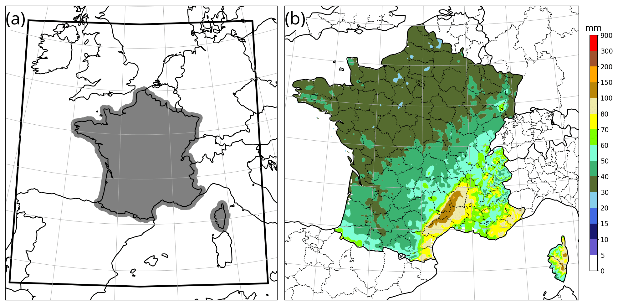
Figure 1(a) AROME computational model domain (black line) and verification area (grey shading), (b) The 6 h climatological precipitation quantile corresponding to a 5-year return period, according to the SHYREG climatology.
2.1 Numerical prediction system
This study is based on an archive of probabilistic forecasts of total precipitation (surface accumulation of rain, snow, and graupel) from the operational Applications of Research to Operations at Mesoscale-Ensemble Prediction System (AROME-EPS) deployed over Europe by Météo-France. Accumulation is considered over 6 h (unless otherwise mentioned) and indexed by the end time of the accumulation interval. The ensemble contains 17 members: an unperturbed control run called deterministic AROME and 16 perturbed members. The numerical prediction model is AROME configured over western Europe (Fig. 1a) with a 1.3 km horizontal resolution and 90 vertical discretization levels. AROME is a convection-permitting atmospheric model with non-hydrostatic dynamics and physical parametrizations of cloud and precipitation microphysics, radiation, sub-grid turbulence, shallow convection, and surface interactions as described in Seity et al. (2011) and Termonia et al. (2018). The deterministic AROME forecasts start from the analysis of a 3D variational data assimilation system (Brousseau et al., 2011). Its large-scale boundary conditions are taken from the global Action de Recherche Petite Echelle Grande Echelle (ARPEGE) prediction system of Météo France.
Perturbed AROME-EPS members start from the deterministic initial state to which perturbations from an ensemble data assimilation system are added. They also use large-scale boundary conditions from the global Prévision d'Ensemble ARPEGE (PEARP) prediction system of Météo France, as described in Descamps et al. (2007) and Termonia et al. (2018). Perturbed surface conditions are documented in Bouttier et al. (2016), and forecast equations are modified by a stochastic perturbation (SPPT) scheme (Bouttier et al., 2012).
The dataset used in this paper is a subset of the operational productions. It covers the period from July 2022 to September 2023, with one 17-member ensemble per day issued from the 21:00 UTC analysis and available for use about 2 h after analysis time. Unless otherwise mentioned, the forecast ranges considered are 9 and 21 h after analysis. They are spaced by 12 h in order to minimize effects from the diurnal cycle. Each accumulated precipitation forecast field is interpolated by a nearest-neighbour algorithm to a regular 0.025° × 0.025° latitude–longitude grid. The available verifying observations (described in the next section) are located well inside the model computational domain.
2.2 Observations and neighbourhood postprocessing
Precipitation forecasts are verified against a truth provided by the 1 km resolution hourly ANTILOPE precipitation analysis (Laurantin, 2013). ANTILOPE merges accumulated precipitation estimated from radar reflectivity observations (Tabary, 2007; Tabary et al., 2013) with rain gauge data. Verification statistics are computed in the area depicted in Fig. 1a, where the ANTILOPE analysis quality is deemed similar to rain gauge measurements because it benefits from good radar coverage and relatively dense in situ reports. The climatology of high precipitation is not homogeneous over the verification area: as shown by the map in Fig. 1b, the heaviest precipitation events tend to occur in the southeastern Mediterranean region. This map was extracted from the SHYREG climatology (Arnaud et al., 2008), which blends an interpolation of rain gauge observations with a statistical model of extreme values.
The ANTILOPE fields are thinned to a 10 km resolution in order to produce pseudo-observations with minimal error correlations between neighbouring reports. It leads to approximately 6800 observation points; i.e. the dataset comprises 60 million model–observation pairs.
Previous studies of precipitation forecast performance have applied bias correction to alleviate systematic errors in model output, for instance using probability matching (e.g. Clark, 2017). Biases in the high-precipitation forecasts have been diagnosed in terms of the relationship between the highest observed and forecast quantiles in Fig. 2, which shows that relative biases are under 20 % up to 35 mm of accumulation. Above this, the biases are larger but difficult to remove because they are linked to increasingly rare events. The extrapolation of statistics from moderate to extreme intensities will be further discussed in Sect. 4.
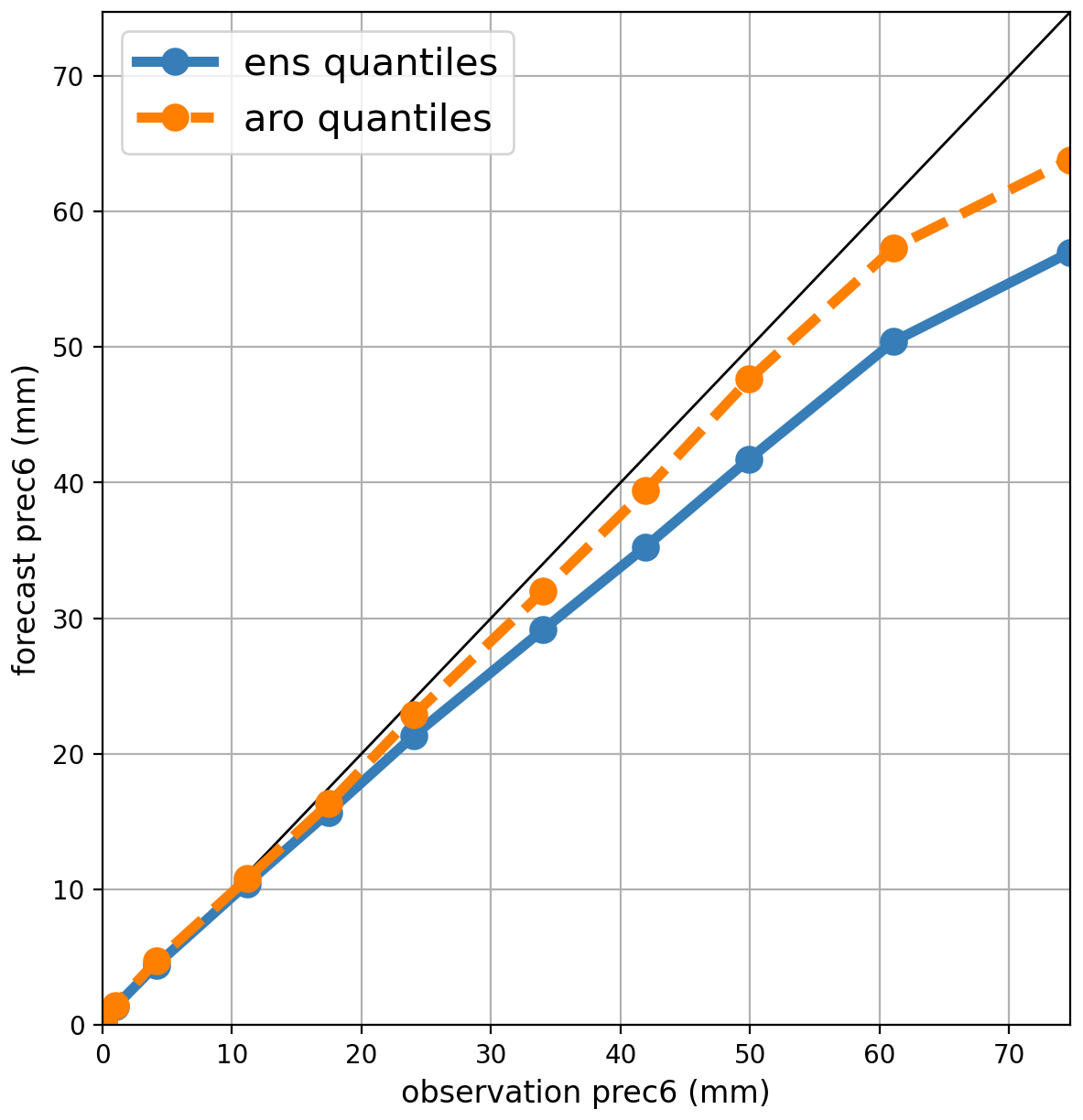
Figure 2Quantile–quantile plot of the AROME ensemble (ens) and AROME control member (aro) precipitation forecast vs. ANTILOPE observations in June 2023.
Probabilistic forecasts will be assessed after filtering at several spatial resolutions, which was shown to have a large impact by Ben Bouallègue and Theis (2014) and Schwartz and Sobash (2017). Severe-weather warnings are usually issued for areas with substantial spatial extent, as in Legg and Mylne (2004). Two spatial aspects of verification will be taken into account in the following score computations.
-
Forecast neighbourhood. Ensemble forecast members are post-processed by a “max-neighbourhood” operator, that is, the forecast at each verification point is replaced by the field maximum in a disc of radius Rf centred on it. Forecast probabilities computed at each point of this post-processed ensemble were called NMAP (neighbouring maximum ensemble probabilities) in Schwartz and Sobash (2017). This operation blurs small-scale detail from the model output while preserving local precipitation maxima. A similar technique was used in Bouttier and Marchal (2020) and shown to be effective at extracting skilful information from ensembles of fields with very-small-scale features.
-
Verification neighbourhood. The NMEP probabilities at each verification point are compared to ANTILOPE observations to which the max-neighbourhood operator is applied with a radius Ro that may differ from Rf. The purpose of observation filtering is to introduce spatial tolerance when comparing forecasts to observations. This procedure was called upscaled verification in Ben Bouallègue and Theis (2014).
As recommended by Schwartz and Sobash (2017), we will set Rf=Ro in most of this paper, except when investigating the potential of relaxing this constraint in Sect. 4.
2.3 Definition of performance scores
The value of 6 h precipitation forecasts will be measured by user-oriented objective scores designed to represent the needs of two hypothetical users:
-
User L (for low) is interested in threshold exceedance of low to moderate precipitation intensities at the highest-possible spatial resolution and wishes to avoid missed events as much as false alarms. We will characterize the corresponding forecast performance using the equitable threat score (ETS) with an arbitrary intensity threshold of 4 mm, which corresponds to fairly common rainfall in the studied area.
-
User H (for high) is interested in the occurrence of more intense and impactful precipitation, can tolerate more false alarms than missed events, and aims to issue high-precipitation warnings at a resolution of 30 km. User H will consider a forecast at any given point to be satisfactory if the predicted precipitation intensity was observed within a 30 km radius. This objective will be modelled by the F2 score using neighbourhoods Rf=Ro = 30 km and an arbitrary intensity threshold of 30 mm, which is reached much more rarely than 4 mm but is frequent enough to produce robust statistics with our dataset.
The ETS and F2 scores are applied as follows: probabilistic forecasts are generated at each verification point by counting the proportion of members that exceed the chosen intensity threshold. Since the number of ensemble members is small, each discrete set of member values will be converted (or dressed; Broecker and Smith, 2008) into continuous probability density functions by convolution with a multiplicative triangular kernel of predefined width. When scoring 17-member ensembles, we will set the kernel width so that its standard deviation is 20 % of the member value. When scoring deterministic forecasts, we will use a standard deviation of 40 %. As reported at the end of Sect. 3, the results presented in this study have little sensitivity to this dressing step; its purpose is to produce smoother score displays than the undressed forecasts.
The aim of this work is to assess the value of deterministic forecast decisions based on ensemble output, a process modelled as a yes forecast of high precipitation when the forecast probability of an event of interest exceeds some probability threshold. Note that the probability threshold (also called the operating threshold in the ROC diagram; Jolliffe and Stephenson, 2011) should not be confused with the precipitation exceedance threshold (in mm) used to define the forecasted event. As noted by Joslyn et al. (2007), Pappenberger et al. (2013), and Demuth et al. (2020), thresholding forecast probabilities is a common decision-making technique when using ensemble forecasts. For the moment, we will treat the probability threshold as a tunable parameter of the forecast procedure. A method to choose its value will be proposed in Sect. 3.
Using the probability threshold, forecast probabilities are converted into deterministic yes/no point forecasts. Their verification against observations leads to the contingency matrix (also called a confusion matrix) that counts forecast successes and failures. For any set of forecast–observation pairs, the counts are computed in terms of the event “precipitation exceeded the intensity threshold” as four categories:
- a.
-
the event was forecast and observed (a hit),
- b.
-
the event was forecast but not observed (a false alarm),
- c.
-
the event was observed but not forecast (a miss), and
- d.
-
the event was neither observed nor forecast (a correct negative).
The confusion matrix can be visualized as follows.
Its coefficients are used to define the scores
The ETS gives similar weights to b and c, whereas F2 gives 4 times more weight to c than to b. The F2 score embodies of user H's tolerance of false alarms, with a target ratio of 4 times more false alarms than missed events. A generalized version of the F2 score could be used for other target ratios. The confusion matrix can be summarized by various other performance metrics such as the following.
- -
-
Forecast frequency bias. ,
- -
-
Hit rate. , also known as the true-positive rate or recall,
- -
-
False discovery rate. , also known as the probability of false alarm or false-alarm ratio,
- -
-
Probability of false detection. , also known as fallout or the false-alarm rate.
We shall avoid using the phrases false-alarm rate and false-alarm ratio given the confusion surrounding these terms, as explained in Barnes et al. (2009).
3.1 Optimization for user L
Ensemble prediction produces forecast probabilities, which leaves it up to the user to convert them into categorical decisions. Here, we will model a binary decision process by thresholding the probabilities, and we propose to define the threshold p, or decision threshold, as the solution popt of an optimization process that maximizes the value of the forecast to the user. For each possible p value, one can associate a set of binary forecasts that leads, through comparison with observations, to a contingency matrix with coefficients (). The ETS and F2 metrics computed from this matrix can then be regarded as functions of p. During rainy events, state-of-the-art numerical weather prediction models normally perform better than the trivial forecasting strategies implied by p=0 (always predict rain) and p=1 (never predict rain). Hence, between 0 and 1, the functions ETS(p) and F2(p) will have a maximum popt, the optimal decision threshold. The respective values ETS(popt) and F2(popt) represent the best value that users can expect to obtain from ensemble forecast output, so they can be regarded as benchmarks of predictive skill. We shall show below that the computation of popt is robust enough to be used as a decision tool for various types of users and events, including high precipitation.
The popt optimization for a such a forecasting process can be summarized as follows:
-
obtain member fields from the ensemble prediction;
-
apply the neighbourhood operator with radius Rf to each field;
-
at each point, build the discrete distribution of predicted values;
-
apply the dressing operator to each distribution;
-
at each verification point, apply the neighbourhood operator with radius Ro to the corresponding observation field;
-
for each possible probability threshold p and at each verification point, compute whether the forecast probability of the event exceeds p and increment the confusion matrix coefficients () according to whether the event was observed and/or predicted; and
-
once the matrix has been computed over the whole learning dataset, set popt as the p value that maximizes ETS(p) or F2(p).
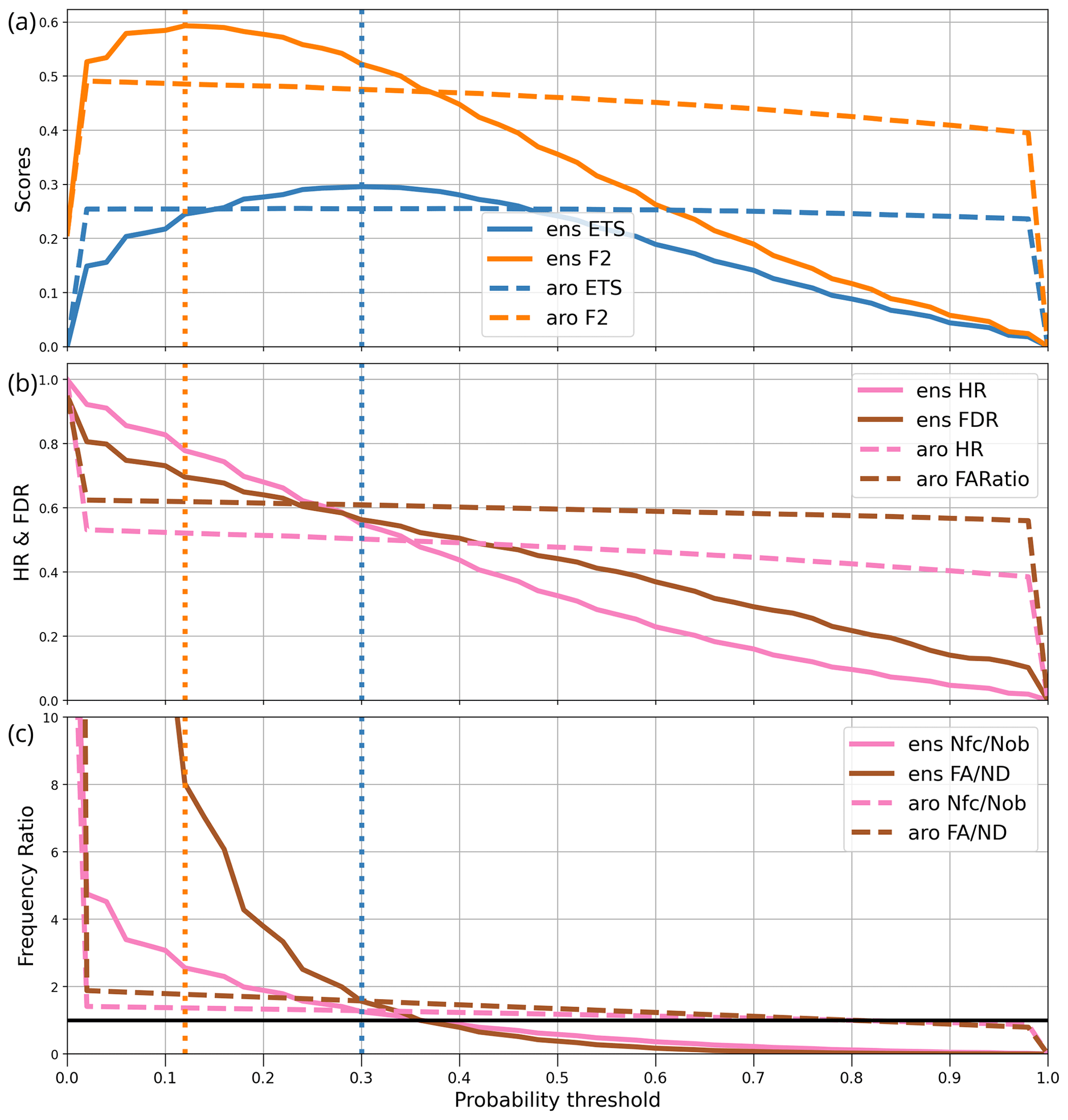
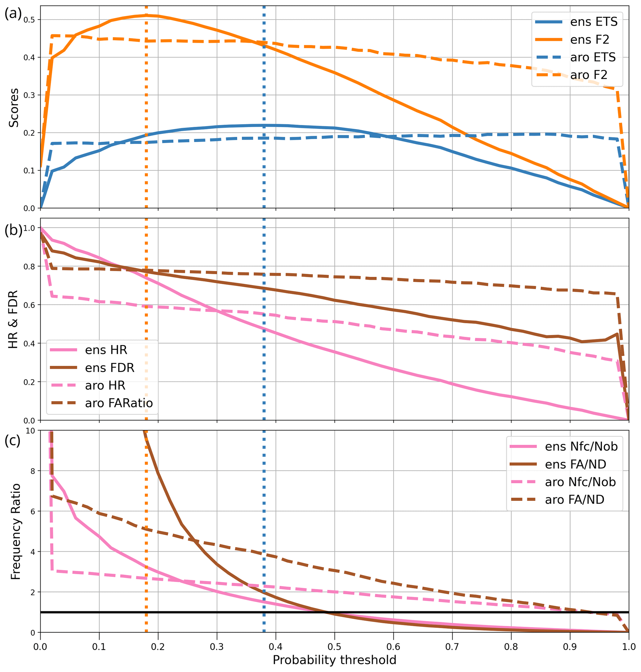
Figure 3Verification statistics of precipitation post-processed over June 2023 for user L as a function of probability threshold. For the AROME-EPS ensemble (ens) and the AROME (aro) deterministic forecast, the curves show (a) the ETS and F2 scores, (b) the hit rate (HR) and false discovery rate (FDR), and (c) the frequency ratios of forecasts to observations (Nfc/Nob) and of false alarms to non detections, i.e. missed events (FA/ND). The vertical dotted lines indicate the optimal decision thresholds for the ETS (orange) and F2 (blue) scores. The horizontal black line in panel (c) indicates the value of 1.
As an example, the computation of popt for user L is illustrated in Fig. 3 over June 2023: the precipitation threshold is set to 4 mm and the neighbourhood radii Rf and Ro to zero. The computation is performed with two numerical prediction systems: the 17-member AROME-EPS ensemble and the deterministic AROME forecast. Both systems are post-processed by the dressing and neighbourhood operators described in Sect. 2. The graphs show various performance diagnostics as a function of the probability threshold p, for all p values between zero and 1 in steps of 0.02.
The top panel of Fig. 3 shows that for AROME-EPS, ETS(p) and F2(p) are broadly concave curves with different popt: popt(F2) is lower than popt(ETS), which reflects the fact that F2 allows more false alarms than ETS, so F2-optimal forecasts of the event will be issued if the forecast probability exceeds 0.12 instead of 0.3 as it is for ETS-optimal forecasts. The popt values are represented in Fig. 3 as vertical lines.
In summary, the best way to warn user L of a risk that precipitation will be above 4 mm is to issue a warning when the forecast probability of this event is above popt(ETS)=0.3. If, as will be shown later, these optimal decision thresholds are not very sensitive to the choice of precipitation threshold, then the forecast information may be summarized by the 0.7 quantile, the optimal quantile because .
It is worth noting that the popt computation need not be very precise: given the rounded shape of the ETS(p) curve, any decision threshold between 0.25 and 0.35 will achieve nearly optimal forecasts. Also, popt should not be interpreted as a calibrated probability because the ensemble used is not exactly reliable: popt is only a tool to construct an optimal decision rule for the (post-processed but uncalibrated) ensemble output. An ensemble calibration step could be incorporated into our precipitation postprocessing procedure (e.g. Ben Bouallègue, 2013; Flowerdew, 2014; Scheuerer, 2014). Calibration techniques that simply remap probability values would not improve ETS(popt) because it already is optimal in terms of end-user scores: our optimization includes an implicit calibration of the ensemble output with respect to the targeted user. More sophisticated calibration techniques could be applied to further increase the value of the ensemble forecast output, in which case our procedure can be applied to the calibrated ensemble instead of the raw members.
The dashed lines in Fig. 3 provide a comparison of the ensemble skill with respect to the deterministic model. The F2(p) and ETS(p) curves for the deterministic AROME model are nearly flat, except for the trivial forecasting strategies p=0 and p=1. They have a slight slope because of the dressing step. The AROME-EPS scores are higher than the AROME scores, which demonstrates that even when the end goal is to issue categorical weather predictions, ensemble prediction can provide better forecasts than a deterministic approach if the users know which decision thresholds to use. At non-optimal thresholds, however, the ensemble scores drop below the deterministic ones. In summary, it is necessary to provide users of ensemble output with supporting information such as popt in order to ensure that their forecasts are better than those implied by deterministic models.
Figure 3b and c provides additional information about the forecast performance. The HR and FDR curves show that improved detection is obtained at the expense of more frequent false alarms. The ETS optimum achieves nearly equal frequencies (55 %) for both kinds of errors, which could be regarded as acceptable for most users of light-precipitation forecasts. Lowering the decision threshold would increase detection faster than the false alarms, which is only an improvement for users that favour detection as modelled by F2. The information conveyed by the HR and FDR curves is similar to an ROC curve (Jolliffe and Stephenson, 2011), with key differences.
-
The probability threshold information is hidden in the ROC curve, unless provided by curve labels. Our graphs show its relationship with performance statistics, allowing the user to understand the implications of basing decisions on a particular threshold.
-
We illustrate the prevalence of false alarms using the FDR statistic instead of the POFD because the latter collapses to very small values for heavy precipitation, since the frequency of correct non-event forecasts (d in the confusion matrix) tends to be very large. This occurs because non-occurrence of high precipitation is trivial to predict in a majority of weather situations that are almost certainly dry. Correct non-event forecasts in these cases imply no practical predictive value. In the ROC diagram, large d values lead to a nearly vertical ROC curve that overemphasizes detection skill at the expense of false alarms. This is undesirable because even when predicting rare events, the frequency of false alarms must be limited to avoid the loss of user confidence in the forecast products (Roulston and Smith, 2004). Using FDR instead of POFD avoids this problem.
Figure 3c shows the forecast bias and the ratio of false alarms to missed events (ratio from the confusion matrix). It indicates that the ETS-optimal decision strategy yields forecasts that over-forecast the event by about 20 %. It also produces more frequent false alarms than missed events, which may seem counter-intuitive because the ETS score equation puts equal weight on both kinds of errors. The explanation is that this strategy produces a larger number of correct forecasts (coefficient a) than the threshold that equalizes b and c. The graphs show, however, that the strategy that produces bias-free forecasts (with p=0.35) is still quite acceptable because its ETS is only slightly lower than ETS(ppopt; by about 5 %).
In summary, we have shown that according to the June 2023 dataset, the optimal forecast strategy for user L is to set the decision threshold to popt(ETS)=0.3, which implies over-forecasting the event (rr6 > 4 mm) by 20 %, with a hit rate and probability of false alarm around 55 %.
3.2 Optimization for user H
The same methodology is now applied to user H, modelled by a precipitation threshold of 30 mm in 6 h with forecast and verification neighbourhood radii Rf=Ro = 30 km. It leads to the plots in Fig. 4. The overall shapes and values of the ETS and F2 score curves are similar to Fig. 3. User H is more tolerant of false alarms, and the optimal decision threshold for AROME-EPS forecasts is popt(F2)=0.18. Error statistics are worse than for user L: the hit rate drops to 0.56, while the probability of a false alarm rises to 0.83. The forecast bias becomes substantial, since the event is now forecast 3 times more often than it is observed. False alarms occur 10 times more often than missed events, which is a consequence of using the F2 score. If one constrains the AROME-EPS-based forecasts to be unbiased instead, by choosing decision threshold p=0.38, the false alarms are reduced at the price of a large hit rate drop, to 0.3. It shows that over-forecasting heavy rain events is necessary to achieve F2-optimal forecast performance.
One could argue from Fig. 4 that the deterministic AROME model seems better than AROME-EPS since for p ≃ 0.35 its hit rate and F2 score are better and its bias is lower. Unfortunately, its probabilities of a false alarm are also much higher, so the answer depends on the relative importance given to each metric. In terms of the F2 score, AROME-EPS is a better forecasting system.
In conclusion, we have shown in this section that the proposed forecast optimization strategy works for two very different user types: the optimum scores are well defined, and they both indicate the superiority of decisions based on the ensemble forecast over the deterministic model. The performance of the optimal decision rules seems reasonable for weak precipitation (user L), but it seems lower for higher intensities despite using neighbourhood methods in the verification (user H). The following sections will now investigate the robustness of these conclusions with respect to space resolution, precipitation intensity, forecast range, season, and accumulation time.
3.3 Sensitivity to the ensemble dressing operator
The impact of dressing on the ensemble postprocessing was checked at the 30 mm intensity threshold with a 30 km neighbourhood and a 30 km verification scale. The dressing kernel width was varied from zero to a large value (50 %). Although the dressing improves the hit rate, its net impact on the scores is very small because most forecast errors are false alarms. The optimal dressing values are between 10 % and 30 %, and they only improve the CSI and F2 scores by 0.3 % and 1 %, respectively, compared to not dressing. Larger dressing widths were found to degrade the scores, which suggests that increasing the ensemble spread too much would be detrimental.
Spatial scale is an important aspect of the use and verification of precipitation forecasts (Ceresetti et al., 2012; Mittermaier, 2014; Ben Bouallègue and Theis, 2014; Buizza and Leutbecher, 2015; Schwartz and Sobash, 2017; Hess et al., 2018). The following sensitivity experiments investigate the impact of changing the neighbourhood operators on our results.
4.1 Sensitivity to the postprocessing neighbourhood radius Rf
The optimization procedure has been rerun as in Sect. 3 with AROME-EPS forecasts, with fixed postprocessing parameters except for Rf, the forecast neighbourhood radius, which is varied between zero and 60 km.
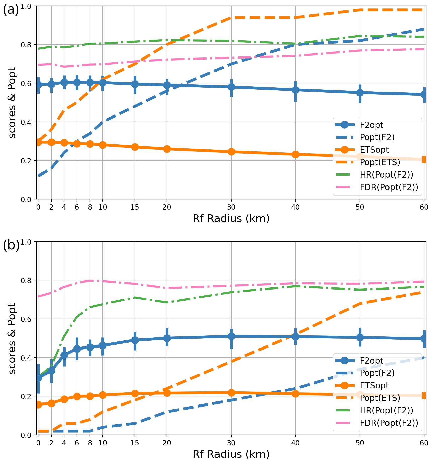
Figure 5Sensitivity of the F2 and ETS scores to the forecast upscaling radius Rf: respective optimum thresholds popt(F2) and popt(ETS), optimum scores F2opt and ETSopt, and error statistics HR and FDR at the F2 optimum. The statistics are shown for (a) user L and (b) user H. Vertical bars indicate 90 % bootstrap confidence intervals for F2.
The results for user L (Fig. 5a) show that applying a neighbourhood to the forecasts only slightly improves the F2 and ETS scores with Rf values of a few kilometres. One may conclude that spatially filtering weak-precipitation forecasts is unnecessary for user L.
The impact of Rf on user H (Fig. 5b) is much larger. Both F2 and ETS increase with Rf until a plateau is reached above 20 km, followed by a slow decrease above 40 km. Two reasons why Rf is more beneficial for user H than for user L can be proposed. One is the conjecture by Schwartz and Sobash (2017) that the scale at which forecasts are upscaled should be consistent with the verification scale, which is the grid scale for user L and 30 km for user H. Another explanation is that 6 h precipitation errors above 30 mm are (in our dataset) mostly caused by thunderstorms with large location uncertainties. Most weak precipitation points are driven by more predictable synoptic fronts. Thus, precipitation location errors seem to affect user H proportionally more than user L.
Two practical conclusions can be drawn. One is that applying a forecast neighbourhood is beneficial when predicting high precipitation, and its radius Rf should be set to values that are not too different from Ro. We have checked (not shown) that this result holds for other precipitation thresholds and for verification radii Ro. The other notable result is that popt is very sensitive to Rf: wider forecast neighbourhoods imply higher probability thresholds because the max-neighbourhood operator widens the areas covered by the highest precipitation, which increases false alarms. As Rf increases, popt increases as well to compensate for this effect. Thus, when using neighbourhood postprocessing, one needs to be careful to adjust popt as a function of the radius.
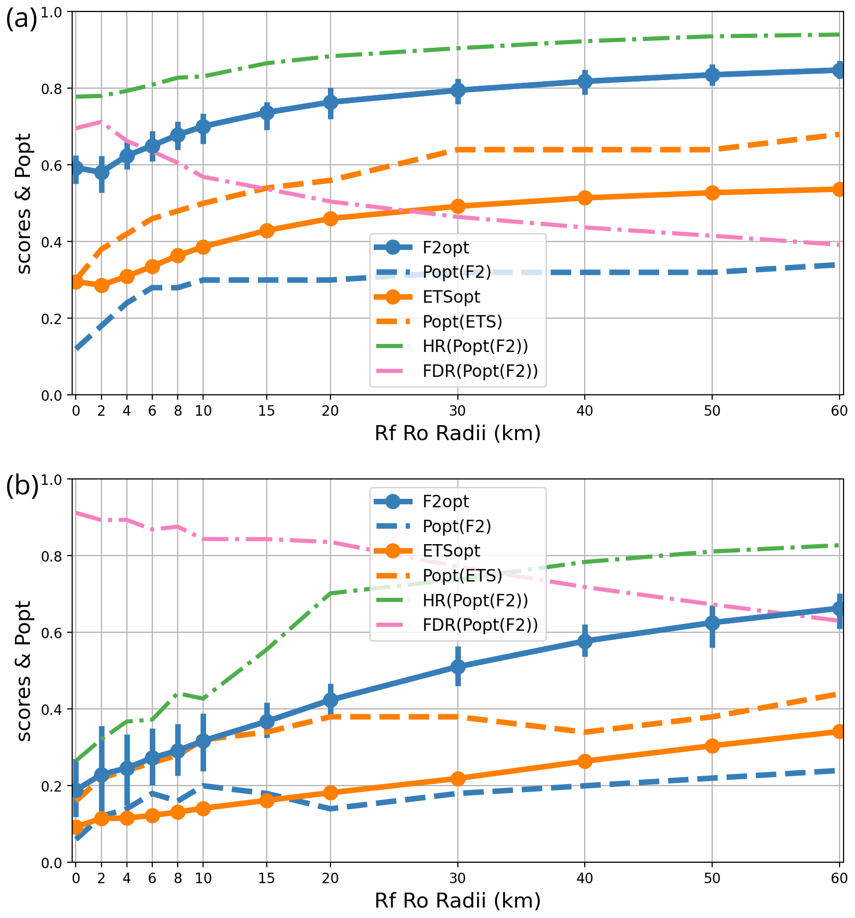
4.2 Sensitivity to the verification radius Ro
The previous study investigated the optimal forecast neighbourhood Rf for users with a fixed verification radius Ro. Here, we check how forecast scores change if the forecasts are verified at different resolutions. In particular, what happens if user H uses forecasts at a higher resolution than Ro = 30 km? To answer, a sensitivity study with respect to Ro is now carried out as in the previous paragraph, except that we keep Rf=Ro, given that this choice of Rf was shown to be optimal in the previous section. We checked that Rf=Ro remains an optimal Rf setting for other choices of Ro, but the corresponding plots are not presented for the sake of conciseness.
The results are shown in Fig. 6 using the 4 and 30 mm precipitation thresholds. In both cases, forecast scores F2 and ETS strongly increase with verification scale, which corresponds to the double-penalty effect mentioned in the introduction. For instance, in terms of the F2 metric, 30 mm forecast accumulation is predicted 3.5 times better at the 80 km scale than at the model grid scale, and both hit rate and false-alarm statistics degrade quickly when changing to finer resolutions. The hit rate drops sharply at scales below 20 km, which can be regarded as the finest resolution at which intense precipitation can be skilfully predicted by the AROME model.
At lower precipitation intensities, the dependency on resolution is similar but weaker: at the 4 mm threshold, the ETS metric is only 1.6 times better at the 80 km scale than at the model grid scale. In other words, precipitation is more predictable at larger scales than at smaller ones, which is consistent with the findings of Buizza and Leutbecher (2015): the predictability of atmospheric variables increases with the horizontal scale considered. This scale dependency is most pronounced for the highest-intensity precipitation events, which can be attributed to their larger location errors.
Two practical conclusions can be drawn. First, if one wants forecasts to meet some minimum accuracy requirements, one should not use model output at too-fine resolutions because the finest details tend to have large forecast errors. Second, because popt has little sensitivity to Ro above 15 km, it can be considered independent from the scale at which forecasts are used once the finest unpredictable details have been filtered out.
In this section, the extrapolation of the previous results to the highest-available precipitation intensities is investigated. The postprocessing and verification radii are kept at Rf=Ro = 30 km, which has been shown to be a satisfactory setting for a wide range of intensities. The 6 h precipitation threshold is varied between 1 and 80 mm. Above ∼ 60 mm, forecast information is valuable because catastrophic consequences begin to occur (with a return period of several years; see Fig. 1b), but the number of independent cases available to compute statistics decreases rapidly. The intent is to assess whether the relatively robust statistics shown in previous sections (popt in particular) can be extrapolated to higher intensities that occur too rarely for direct statistical treatment. As our focus is on heavy precipitation, and it has been shown that forecast accuracy is very low at verification scales below 20 km, we only present results for user H at a verification scale of Ro = 30 km.
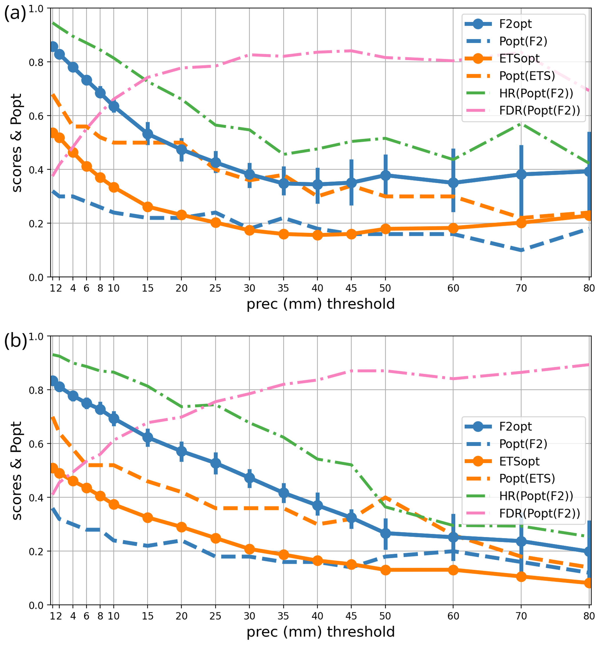
Figure 7As in Fig. 5 but as a function of the precipitation intensity threshold for user H over 2 periods: (a) September to November 2022 and (b) May to July 2023.
Figure 7 shows the precipitation forecast performance as a function of intensity. The statistics have been gathered over two independent 3-month periods, as opposed to 1 month in Sect. 3, in order to improve the sampling of higher-intensity events. Even so, there is substantial sampling uncertainty at 60 mm and above, as illustrated by the 5 %–95 % bootstrap confidence intervals displayed on the F2 curves.
In terms of sample size, one can note that in each period the number of observation points that exceed threshold intensities (20, 40, 60, or 80 mm) is on the order of 30 000, 6000, 1400, or 500 points. Since neighbouring data points are likely to have correlated error statistics, the actual amount of independent data is likely to be at least 1 order of magnitude smaller, such that 80 mm can be regarded as an upper limit on the intensities at which our statistics are likely to be robust.
During both periods, there is a steep degradation of the scores as the intensity threshold increases. Light accumulation is much more predictable than the heavy accumulation events that exhibit more than 80 % of false alarms and less than 50 % detection rates at the highest thresholds. A user that requires better forecast performance than these values may conclude that numerical predictions are not suitable and that forecast decisions should instead be based on other data sources like nowcasts or observations.
Both tested periods have fairly similar statistics, and the score variations are simultaneously caused by detections and false alarms. Interestingly, the autumn scores are nearly constant over 30 mm, but spring scores keep decreasing at all thresholds. A possible explanation is that heavy precipitation in autumn is more likely to be caused by orographically forced convection in the Mediterranean area. These events are driven by slowly evolving, highly coherent weather patterns (Amengual et al., 2021; Davolio et al., 2013; Nuissier et al., 2016; Caumont et al., 2021) with comparatively high predictability. As already implied by Fig. 1b, precipitation characteristics are completely different between the northern part of France and the Mediterranean region, which probably leads to the variations in the performance scores.
The popt statistic strongly depends on intensity, but its variations are smooth: for F2, it is close to 0.3 at low intensities, and it decreases to about 0.15 at 80 mm (depending on the period). Above 30 mm, popt values are nearly constant and vary by less than 5 %, which is inside the tolerance intervals identified in Sect. 3. Thus, it seems that issuing precipitation forecasts using the 0.85 quantile of the ensemble forecast is a nearly optimal strategy for all precipitation above 30 mm if the aim is to maximize the F2 score at a minimum scale of 30 km.
This section investigates the robustness of the previous results with respect to three aspects of the forecasts: forecast range, season, and accumulation length. The diurnal cycle will be studied through the forecast range dependency since all forecasts considered start from the same time of day.
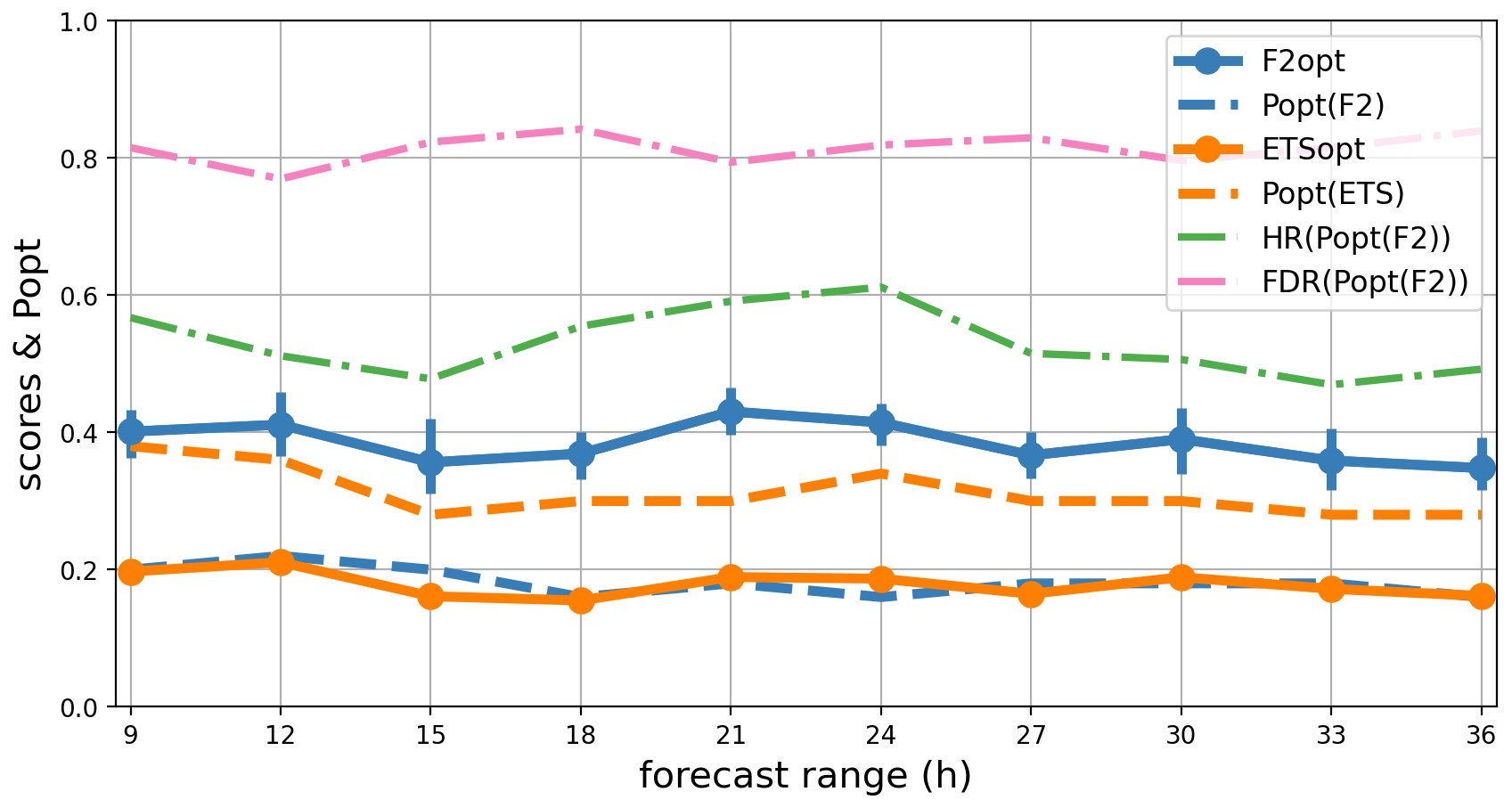
Figure 8As in Fig. 5 but as a function of forecast range and on average over 1 year for user H.
6.1 Sensitivity to forecast range and diurnal cycle
Figure 8 shows the forecast statistics of 6 h accumulation for user H, averaged over 14 months (July 2022 to September 2023), and stratified versus the AROME-EPS forecast range. More forecast ranges have been taken into account in this plot than in previous sections in order to adequately sample the time evolution.
The shortest range considered is 9 h (6 h accumulated precipitation at ranges from 3 to 9 h) because AROME-EPS operational production typically takes a little over 2 h to run in real time, so ranges smaller than 2 h are useless. Second, the first time steps have poor error statistics because of diabatic spin-up effects in the AROME model. Spin-up occurs because of physical inconsistencies in data assimilation and in initial ensemble perturbations (e.g. Bouttier et al., 2016; Brousseau et al., 2011; Auger et al., 2015). Although the longest operational forecast range is 51 h, to save computation time, our study is limited to a range of 36 h. The range interval used for this study (3 to 36 h) is long enough to sample the whole diurnal cycle.
Figure 8 shows that the scores and statistics are nearly independent of range from 9 to 36 h. There is a small decrease of less than 10 % in F2, ETS, hit rate, and popt. A hint of the diurnal cycle is visible. The lower predictability at ranges from 15 to 18 h (12:00 to 15:00 LST, local solar time) is probably due to diurnal development of convection during the warm season. Nevertheless, the diurnal cycle is too small to have practical significance.
Published verifications of ensemble predictions have usually shown that their scores decrease over ranges of several weeks due to chaotic error growth during the forecasts (Buizza and Leutbecher, 2015). During the first forecast day, the relative decrease in the scores tends to be small (Bouttier et al., 2016). Thus, over the ranges studied here, chaotic forecast error growth is hardly visible because it occurs over longer timescales. At short ranges, the quality of the AROME-EPS initial conditions is driven by the application of relatively large initial ensemble perturbations (Bouttier et al., 2016), which lead to a comparatively slower error growth than in nowcasting-oriented forecast systems (Auger et al., 2015), where the emphasis is on the consistency of the initial conditions with the latest observations. Combining nowcasting information with the AROME-EPS model could probably improve the short-range forecasts, as suggested by Nipen et al. (2011).
In conclusion, for practical purposes one can consider the scores and optimal thresholds as being nearly independent from the forecast range and time of day.
6.2 Seasonal dependency
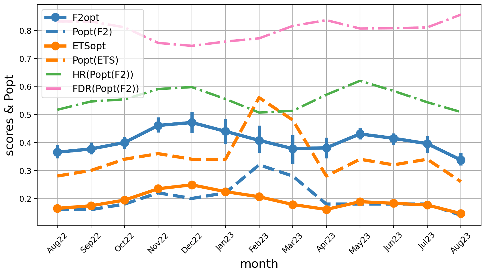
The error statistics are now shown as a function of the forecast starting date over 15 months in Fig. 9; a 3-month running average has been applied. Again, the variations are small, apart from a kink around February and March 2023. It was an exceptionally dry period, so this feature does not seem significant. It suggests that the number of events should be taken into account when defining the time intervals over which aggregated statistics are derived. The general shape of the curves seems driven by the strong natural variability that occurred at the monthly timescale during the period: the weather was dry except for a few rainy spells during August–November 2022, May–June 2023, and Sep 2023. The conclusion is that if there is a seasonal cycle in the scores and in popt, it cannot be clearly identified by this study. A longer dataset covering several years would be needed in order to average out the natural variability that occurs from month to month, to identify the seasonal dependency in the scores and the associated popt thresholds. This seasonal dependency could be very different from region to region.
6.3 Sensitivity to accumulation timescale
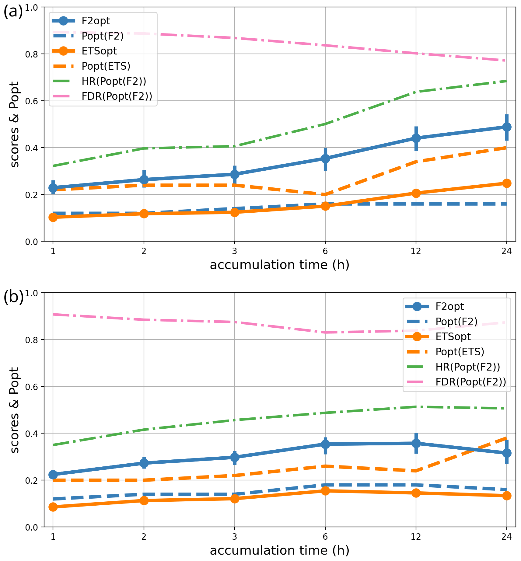
Conceptual models of turbulent flows suggest that smaller-scale features have shorter lifespans and lower predictability than larger-scale ones; this view is supported by atmospheric predictability studies (e.g. Buizza and Leutbecher 2015). Hence, one suspects that the precipitation forecast scores and the associated decision thresholds (popt) depend on the length of the accumulation windows, which act as a low-pass time filter. To check this hypothesis, the same 24 h interval of forecast ranges from 3 to 27 h has been split into six different partitions: 1 × 24 h, 2 × 12 h, 4 × 6 h, 8 × 3 h, 12 × 2 h, and 24 × 1 h. The forecast error statistics have been computed for accumulation over these intervals.
Table 1Precipitation thresholds with a 5-year return period used in Fig. 10.
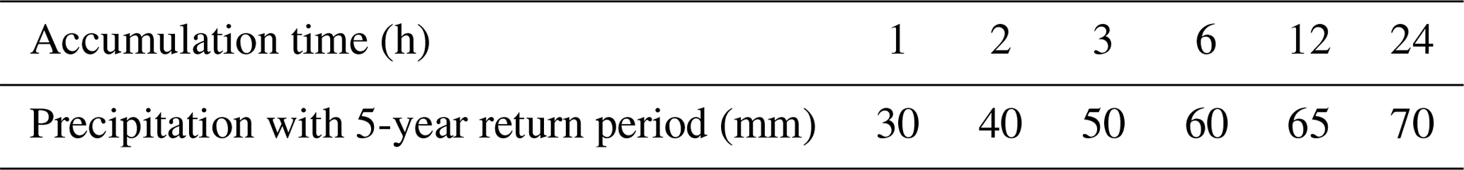
For each accumulation period, the intensity thresholds for computing scores were adjusted in order to represent similar levels of severity, defined as the spatial median of the 5-year return period of precipitation in the SHYREG climatology (Fig. 1b). The thresholds used are shown in Table 1.
The scores and popt statistics have been computed over two independent 3-month periods, chosen for their relative abundance of precipitation: September to November 2022 and May to July 2022. The first one was characterized by a strong synoptic forcing with intense orographically forced precipitation events. The second one had mostly weakly forced thunderstorms.
The dependency of the statistics on accumulation time is shown in Fig. 10. During the September–November 2022 period, longer accumulation is much more predictable than shorter accumulation (the F2 and ETS scores are higher, the hit rate is higher, and the probability of a false alarm is lower). Accordingly, popt is nearly twice as high for a 24 h accumulation as for a 1 h accumulation.
This result is important for hydrological applications because it indicates that flood warnings driven by such an ensemble prediction system should use probability thresholds popt that depend on the timescale that is most relevant to each river system. Our results show that floods that depend on timescales longer than 6 h can have forecast error statistics that are quite different from shorter ones. Heavy-rain warnings for accumulation over 1 to 3 h needs to be triggered at very low probability levels (10 % or less) because the hit rates are quite low, and it will cause a lot of false alarms (as illustrated by the FDR curve). Forecasting of such short-timescale events should probably rely on nowcasting products and/or be used with some time tolerance.
During the May–July 2023 period, the statistics are nearly independent from the timescale and not better than the shortest (i.e. the worst) timescales of the other period. A possible explanation is that this period is dominated by intense but non-stationary rainy systems such as thunderstorms: accumulation over longer periods is produced by multiple short-lived, unpredictable convective systems, unlike the persistent rain from long-lived coherent weather systems.
The conclusion is that longer accumulation is generally more predictable than shorter accumulation and that this information could be used to optimize warning decisions, particularly regarding flood risks. Unfortunately, this effect seems to depend on the period considered, so a more elaborate model of this dependency (possibly with predictors of weather type) should be introduced into the popt computations before this information can be confidently used in practice.
The previous results suggest that automatic precipitation exceedance warnings could be obtained from the optimal ensemble postprocessing parameter values using probability threshold popt. Human forecasters are usually responsible for issuing severe-weather warnings on the basis of their expert knowledge. Hence, they need to understand the meteorological context of the numerically predicted information, which can be visualized from weather maps. Forecasters on duty may not have the time to look at each member, which tends to be a tedious task: there is active research on designing efficient graphical products to present ensemble forecast information (Demuth et al., 2020). Here, we focus on the problem of graphically representing the fact that a high-precipitation warning should be issued because the ensemble forecast probability is larger than popt. Probability exceedance maps are not ideal because they do not show a physical parameter (the probability value), and they are defined with respect to a fixed threshold.
Our results have shown that for high precipitation, popt is a slowly varying function of precipitation intensity, so we propose to summarize the ensemble prediction by maps of (1−popt) quantiles of the post-processed ensemble. These maps show precipitation intensities that have probability popt of occurring. We will call them optimal quantiles for the user for whom popt has been optimized. At each grid point, the optimal quantile is the precipitation value that is most likely to minimize user losses. In our framework, user L should, on average, rely on maps of qL quantiles with with a small neighbourhood (set to Rf= 5 km), which is appropriate for grid point predictions where missed events carry the same costs as false alarms. The optimal quantile for user H is the qH quantile with with a neighbourhood of Rf = 30 km, which is appropriate for severe-weather warnings at this spatial scale, incurring approximately 4 times more false alarms than missed events.
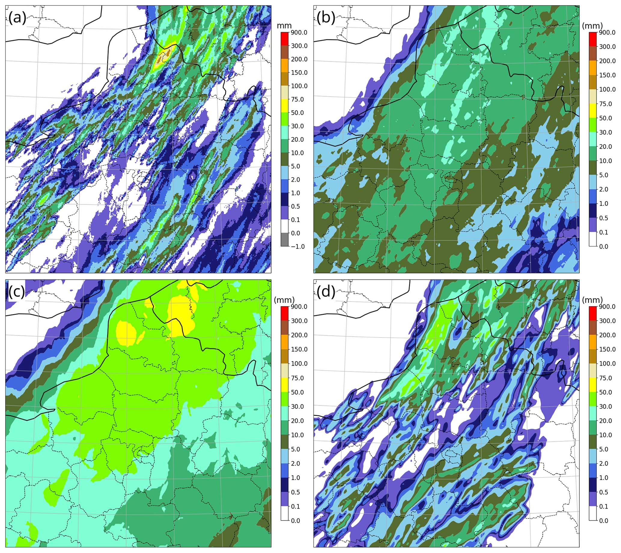
Figure 11Maps of 6 h accumulated precipitation on 20 June 2023 between 12:00 and 18:00 UTC over northern France. (a) Truth provided by the ANTILOPE analysis, (b) qL quantile of the AROME-EPS ensemble 21 h range forecast (0.7-quantile with a 5 km neighbourhood), (c) qH quantile of the same forecast (82 % percentile with a 30 km neighbourhood), and (d) AROME-France deterministic forecast.
The maps are now presented for several test cases. The first one, illustrated in Fig. 11, involved a highly localized flood event at the border between France and Belgium. Observed accumulation exceeding 100 mm was produced by a line of mobile thunderstorms embedded in a synoptically driven cold front. The large-scale features of the front were highly predictable, but the small-scale details were produced by small-scale convection with large uncertainties in location and timing, as reflected in the ensemble spread and in the forecast errors. Although most ensemble members predicted significant precipitation (a 5-year return period was reached by the deterministic AROME forecast), they were all weaker than observed.
The spatial ensemble spread of the predicted thunderstorms was much larger than their size, so that most quantile maps, such as the qL quantile shown in Fig. 11b, did not show precipitation above 30 mm. The qH quantile in Fig. 11c shows much more realistic intensities, as well as a more informative delineation of the areas where severe precipitation is likely to occur. For instance, the qH quantile areas with values above 50 mm correctly framed the observed high-precipitation event (although the peak observed intensity was much higher than predicted), thanks to the combination of the ensemble spread with the neighbourhood postprocessing. Since the qH quantile overestimates precipitation in the central parts of the plotted area, a high-precipitation warning based on qH quantile values above 50 mm would arguably result in many false alarms because of the limited sharpness of the ensemble forecast, but it nevertheless would still contain better information about the areas at risk than the deterministic forecast (Fig. 11d). The latter predicted similar values but much further away (by more than 70 km) from the observed event.
The qL and qH quantile forecasts are quite different from each other, which demonstrates that in the presence of high forecast uncertainties, the optimal forecast can strongly depend on the user for whom the forecast is optimized.
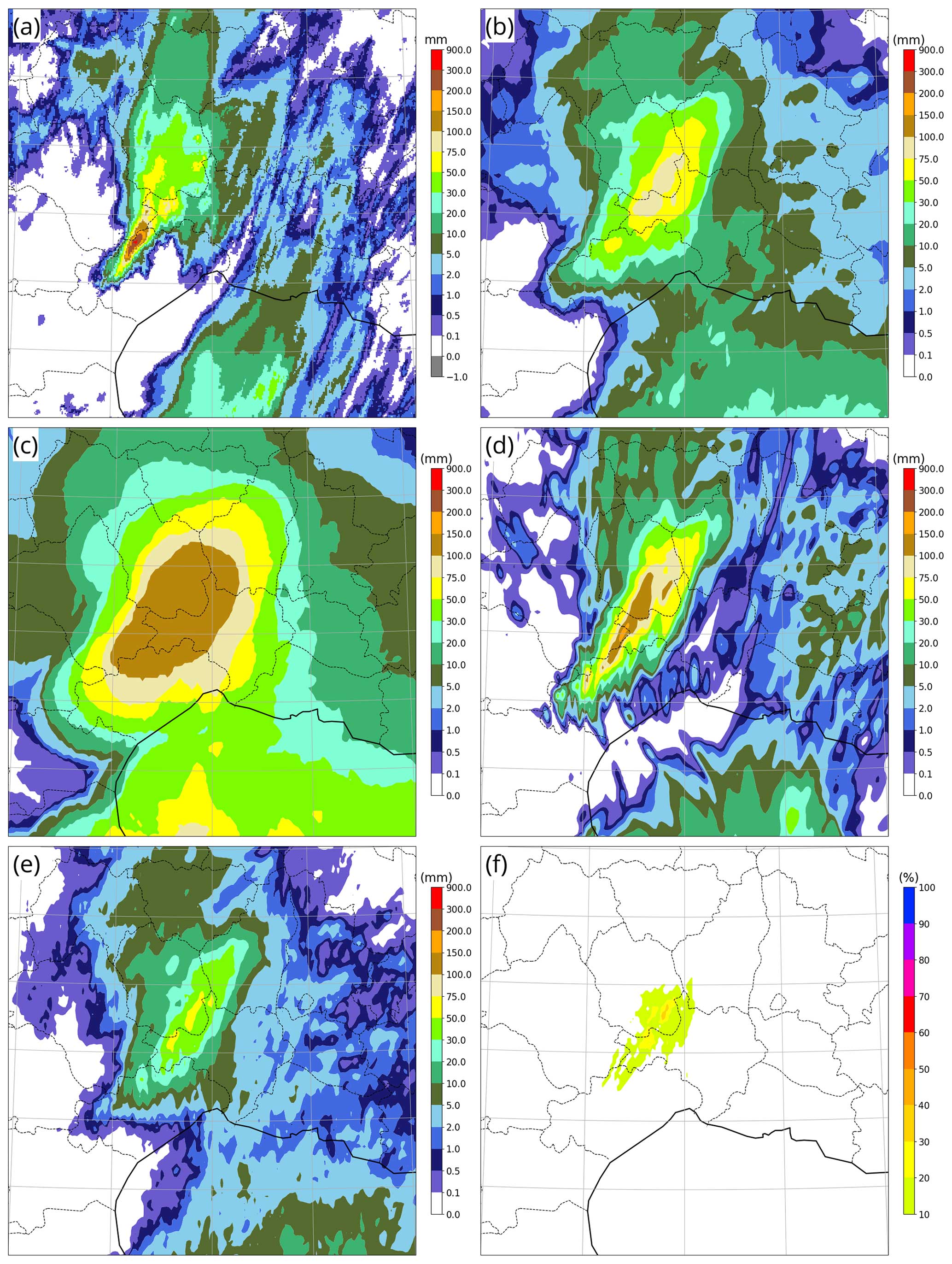
Figure 12As in Fig. 11 but on 16 September 2023 between 00:00 and 06:00 UTC over southeastern France, with two extra panels: (e) median of the AROME-EPS ensemble and (f) AROME-EPS probability that precipitation exceeds 75 mm at each grid point.
The second case, presented in Fig. 12, is typical of flooding events that frequently occur in autumn around the northwestern Mediterranean sea. In such cases, synoptically forced warm and moist low-level onshore winds trigger quasi-stationary convective systems above or near hills. Here, over 300 mm of rain was observed over 6 h in a very localized area (Fig. 12a) in the Cévennes mountains (located where the highest values of Fig. 1b occur). As in the previous case, the qL quantile (Fig. 12b) severely underestimated and misplaced the highest accumulation, while being a rather accurate forecast in weaker-precipitation areas. The qH quantile (Fig. 12d) successfully encompassed the observed high-precipitation event with more accurate values. The deterministic forecast (Fig. 12d) was more precise than the qH quantile in terms of false-alarm avoidance and maximum values, but its peak was located too far north, missing the observed peak by about 20 km. Both qL and qH quantiles are clearly superior to the raw ensemble median (Fig. 12e) and the probability map of exceeding 75 mm (Fig. 12f), both of which failed to convey the risk of damaging precipitation (which occurs beyond 100 mm intensities in this area).
It is not clear whether the best overall forecast was provided by the qH quantile or by the deterministic forecast. The qH quantile detected the whole event at the price of a less-precise framing of the area at risk and of an underestimation of maximum intensities: answering is a matter of preference between detection, false alarms, and peak intensity. The qH quantile produced many false alarms, which may not be acceptable as a warning practice in many meteorological institutes.
The likelihood of high precipitation in this region has a climatological NW–SE gradient (see Fig. 1b), so that the qH quantile forecast could probably be improved (with less blurring) using anisotropic neighbourhoods in this area, to express the fact that location errors are more likely to occur along the SW–NE than along the NW–SE directions.
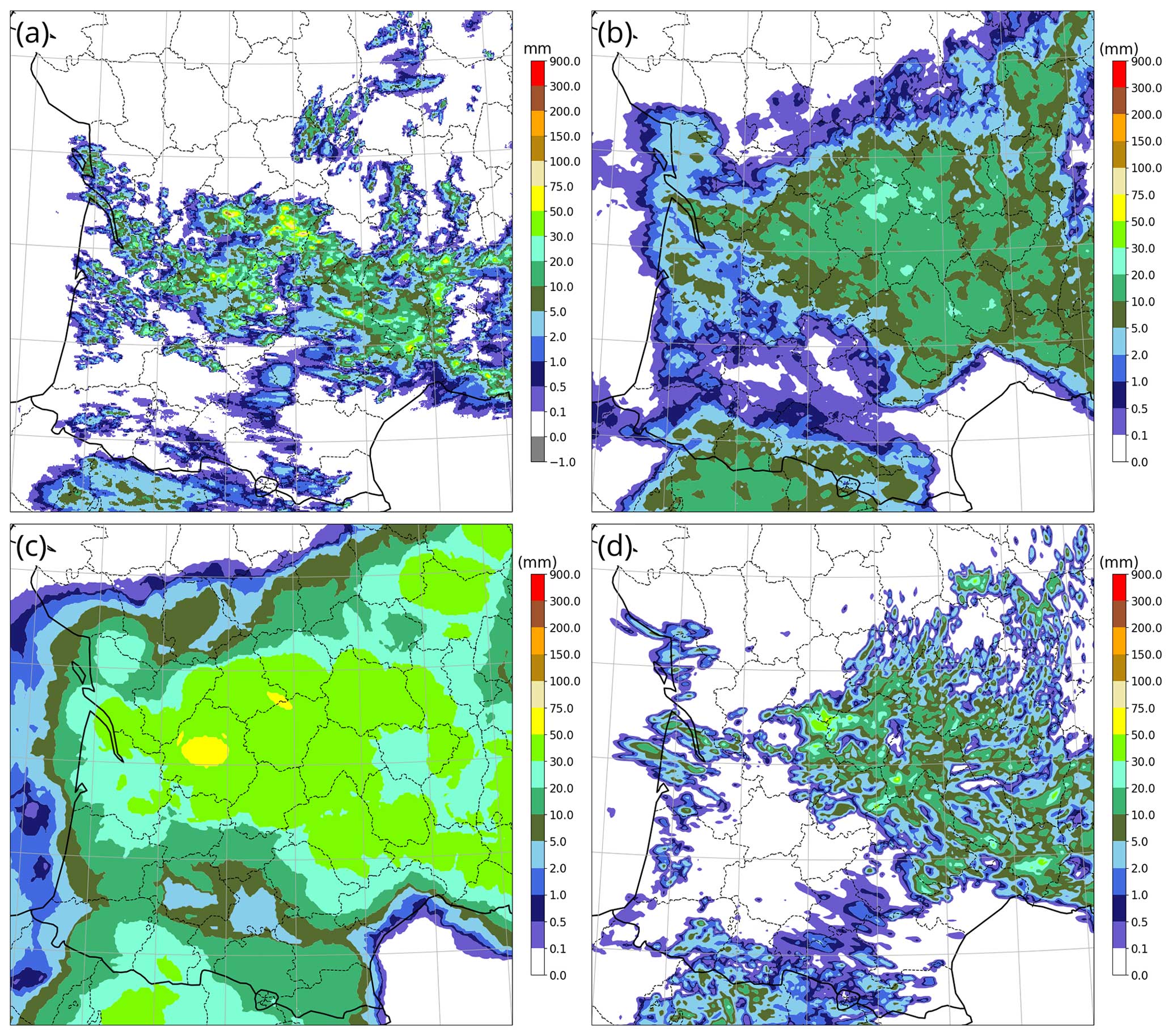
Figure 13As in Fig. 11 but on 22 May 2023 between 12:00 and 18:00 UTC over southwestern France.
The third case, presented in Fig. 13, was an unstructured afternoon thunderstorm case in a convectively unstable air mass. Unlike the previous cases, it was not caused by significant forcing from the synoptic cases or from orography. Many small, quasi-stationary convective cells developed chaotically, some of them leading to considerable accumulation at highly unpredictable locations. The AROME deterministic forecast (Fig. 13d) accurately predicted the precipitation maximum and the overall precipitating region. The texture of the field looked more realistic, with a good prediction of the size of precipitating cells, but their individual locations were generally wrong. There was a general northward shift of up to 100 km. Some large areas that were predicted to be dry actually experienced thunderstorms. The qL quantile (Fig. 13b) correctly smoothed out most random small-scale detail. It was a more satisfactory prediction of rain occurrence than the deterministic forecast, but it severely underpredicted the accumulation from the thunderstorms. Conversely, the qH quantile (Fig. 13c) overpredicted the light-precipitation area, but it correctly delineated the envelope of the high-rain area, with a better indication of the highest-expected accumulation than both AROME and the qL quantile. One can regard the qH and qL quantile maps as being two possible views of the same forecast.
In conclusion regarding the case studies, we have demonstrated that our technique for computing the qL and qH quantiles leads to quite different forecast maps. They both eliminate unpredictable small-scale detail from the member forecasts, as illustrated by the comparison with the deterministic AROME output. Maps of the qL and qH quantiles are very different from each other because they cater to different needs: the qL quantile summarizes information about rain occurrence and light accumulation, whereas the qH quantile suggests a worst-case scenario in terms of extent and amplitude of the heaviest accumulation. The added value of the qL and qH quantile products with respect to the raw deterministic forecast is not always clear: it may not be obvious if the weather situation is highly predictable (e.g. the location of moderate precipitation in Fig. 12) or if all members exhibit the same kind of errors. In the latter situation, similar errors will be found in the post-processed products because our algorithm is not designed to correct for systematic forecast errors.
Visual inspection of other high-precipitation cases has suggested that the qL and qH quantiles do not always convincingly improve over the deterministic forecast but that they do not significantly degrade it either, which suggests that optimal quantiles are a safe way of summarizing ensemble forecasts for users with well-defined objectives.
A data-based ensemble postprocessing method has been presented. It is a generalization of the proposals of Ben Bouallègue and Theis (2014) and Schwartz and Sobash (2017). It takes into account user requirements in terms of target rain intensities and tolerance to false alarms vs. missed events. The aim is to summarize ensemble forecasts for efficient time-critical interpretation and as an input for decision-making, such as high-precipitation warnings.
The method is statistical learning based on forecasts archived over a few months. Its output is a set of optimal decision thresholds expressed as an ensemble probability threshold popt (or, equivalently, an optimal quantile level). The postprocessing combines a probability dressing step, a maximum spatial neighbourhood operator (to represent the effect of location errors), and a probability threshold optimization defined with respect to a user-dependent loss function. The dressing step allows a fair comparison between ensemble and deterministic forecasts. The loss functions model the requirements of two kinds of users based on the ETS and F2 scores. The properties of F2 make it suitable for scoring high-impact weather events with a higher tolerance for false alarms than for event misses.
Using impact experiments, the sensitivity of the popt optimization to several aspects of the postprocessing has been examined to ensure that the procedure is stable and that its sensitivity to the implementation settings is well understood. The value of popt turned out to be sensitive to the choice of loss function, precipitation intensity, and neighbourhood radius but not very sensitive to forecast range, season, and precipitation accumulation time. The popt variation with precipitation intensity is smooth, so it can be extrapolated from the highest intensities allowed by the training sample to the extreme-precipitation forecasts produced by a convection-permitting numerical ensemble. Case studies of high-precipitation events support this extrapolation hypothesis to the extent that for each targeted user, popt-based optimal quantile forecast maps seem to better summarize useful ensemble information than a deterministic control forecast does.
Objective scores of popt-based forecasts are significantly better with an ensemble forecast than a deterministic control forecast. The inclusion of the neighbourhood operator improves forecasts of relatively high precipitation events, but its impact on forecasts of low precipitation is small. The set of forecast ranges considered in our study is too narrow to document the chaotic loss of predictability in medium range (2 to 15 d) forecasts. This loss appears to be negligible from 3 to 36 h.
Three kinds of relative “predictability horizons” for precipitation can be identified: intensity, time resolution, and space resolution. After popt optimization, precipitation forecast skill generally decreases with intensity, with the possible exception of orographically forced events. It increases with accumulation time, although this dependency appears to be situation dependent. It strongly increases with verification scale. These results confirm the physical intuition that larger scales (in space and time) are more predictable than smaller ones. Higher precipitation is less predictable, presumably because it tends to be produced by relatively small-scale weather systems.
The score variations are clearly related to hit rates and probabilities of false alarm, so one can conclude that users expecting forecasts to meet predefined performance requirements should not ask for forecasts on too fine a scale. In particular, high-precipitation-forecast scores drop quickly at scales smaller than 10 to 30 km. Although there is some skill in the prediction of high precipitation, users wishing to base their decisions on confident high-precipitation forecasts (such as emergency services with constrained resources) or forecasters who wish to avoid losing credibility by issuing false alarms too often may conclude that they should not base their forecast decisions on numerical weather prediction and they might prefer to rely on more accurate data sources such as nowcasting.
The postprocessing method proposed here can be regarded as an ensemble calibration, since our popt optimization procedure will compensate for some forecast biases. Standard ensemble calibration methods such as published by Gneiting et al. (2005), Scheuerer (2014) or Flowerdew (2014) have usually been designed to optimize generic aspects of the forecasts. The originality of our work is to directly optimize the postprocessing in terms of user-specific loss functions, which guarantees that they get the best possible information. As our sensitivity and case studies have demonstrated, when forecast uncertainties are significant, probabilistic forecast products strongly depend on the preferences of the users for whom they are designed.
Fundel et al. (2019) and Demuth et al. (2020) pointed out that the variety of user needs is a challenge for communicating forecast uncertainty information. The method outlined in our work proposes to help with this problem by summarizing forecasts using maps of optimal quantiles, which are relatively quick and easy to interpret: they are expressed in physical units and their relationship with the member fields can be intuitively retraced based on popt and the neighbourhood radius. These maps can be generated from limited historical archives. The information they convey is objectively better on average than the corresponding deterministic forecast, and they have the potential to help identify regions where there is a risk of heavy precipitation in various types of weather situations.
Two applications of this work can be envisioned. First, the popt information, in particular as optimal quantile maps, could help human forecasters to quickly access ensemble forecast information in terms of the geographical extent and intensity of high-precipitation events. Second, this information could be included in automated point weather forecast applications to ensure that they convey the risks of high precipitation, even if the forecast accuracy of our algorithm is still probably much lower than what experienced humans can achieve in terms of severe-precipitation warnings.
The proposed technique could be improved in several ways, which is left for future work. For instance, more members could be used, combining multimodel ensembles with lagging. Nowcasting information could be included at the short range. The neighbourhood operator could be made anisotropic and location dependent in order to account for orographic effects. Neighbourhood operators that depend on ensemble spread have been tested by Blake et al. (2018), with encouraging results. More fundamentally, popt could be computed by a regression in a more general statistical model, for instance a convolutional artificial neural network that would include geographical and seasonal dependency and indicators of weather type as predictors, in addition to the precipitation fields used in this study.
The loss function could also be improved to include other measures of forecast quality than the numbers of missed events and false alarms. For instance, it may be helpful to minimize inconsistency between successive forecasts (Demuth et al., 2020), as well as stop the repeated false alarms that can lead to loss of user confidence in the forecasts.
The figures of this article can be regenerated from the data provided on a public repository at https://doi.org/10.5281/zenodo.10420739 (Bouttier and Marchal, 2024), with the exception of Fig. 1b, which uses proprietary data that can be requested from the INRAE institute.
Conceptualization and methodology – FB and HM; investigation, software, interpretation, visualization; and writing – FB. Both authors have read and agreed to the published version of the paper.
The contact author has declared that neither of the authors has any competing interests.
Publisher's note: Copernicus Publications remains neutral with regard to jurisdictional claims made in the text, published maps, institutional affiliations, or any other geographical representation in this paper. While Copernicus Publications makes every effort to include appropriate place names, the final responsibility lies with the authors.
The article was improved by helpful comments from anonymous reviewers.
This work was funded by the French government through Météo France and CNRS.
This paper was edited by Vassiliki Kotroni and reviewed by two anonymous referees.
Addor, N., Jaun, S., Fundel, F., and Zappa, M.: An operational hydrological ensemble prediction system for the city of Zurich (Switzerland): skill, case studies and scenarios, Hydrol. Earth Syst. Sci., 15, 2327–2347, https://doi.org/10.5194/hess-15-2327-2011, 2011. a
Alfieri, L. and Thielen, J.: A European precipitation index for extreme rain-storm and flash flood early warning, Meteorol. Appl., 22, 3–13, https://doi.org/10.1002/met.1328, 2012. a
Amengual, A., Hermoso, A., Carrió, D. S., and Homar, V.: The sequence of heavy precipitation and flash flooding of 12 and 13 September 2019 in eastern Spain. Part II: A hydro-meteorological predictability analysis based on convection-permitting ensemble strategies, J. Hydrometeorol., 22, 2153–2177, https://doi.org/10.1175/jhm-d-20-0181.1, 2021. a, b
Arnaud, P., Lavabre, J., Sol, B., and Desouches, C.: Regionalization of an hourly rainfall generating model over metropolitan France for flood hazard estimation, Hydrolog. Sci. J., 53:1, 34–47, https://doi.org/10.1623/hysj.53.1.34, 2008. a
Auger, L., Dupont, O., Hagelin, S., Brousseau, P., and Brovelli, P.: AROME-NWC: A new nowcasting tool based on an operational mesoscale forecasting system, Q. J. Roy. Meteor. Soc., 141, 1603–1611, https://doi.org/10.1002/qj.2463, 2015. a, b
Barnes, L. R., Schultz, D. M., Gruntfest, E. C., Hayden, M. H., and Benight, C. C.: Corrigendum: false alarm rate or false alarm ratio?, Weather Forecast., 24, 1452–1454, https://doi.org/10.1175/2009WAF2222300.1, 2009.
Ben Bouallègue, Z.: Calibrated short-range ensemble precipitation forecasts using extended logistic regression with interaction terms, Weather Forecast., 28, 515–524, https://doi.org/10.1175/WAF-D-12-00062.1, 2013. a
Ben Bouallègue, Z. and Theis, S.: Spatial techniques applied to precipitation ensemble forecasts: from verification results to probabilistic products, Meteorol. Appl., 21, 922–929, https://doi.org/10.1002/met.1435, 2014. a, b, c, d, e
Blake, B., Cartley, J., Alcott, T., Jankov, I., Pyle, M., Perfater, S., and Albright, B.: An adaptive approach for the calculation of ensemble gridpoint probabilities, Weather Forecast., 33, 1063–1080, https://doi.org/10.1175/WAF-D-18-0035.1, 2018.
Bouttier, F. and Marchal, H.: Probabilistic thunderstorm forecasting by blending multiple ensembles, Tellus A, 72, 1696142, https://doi.org/10.1080/16000870.2019.1696142, 2020. a
Bouttier, F. and Marchal, H.: Dataset and plot generation script for article “Probabilistic short-range forecasts of high precipitation events: optimal decision thresholds and predictability limits”, Zenodo [code] https://doi.org/10.5281/zenodo.10420739, 2024. a
Bouttier, F., Vié, B., Nuissier, O., and Raynaud, L.: Impact of stochastic physics in a convection-permitting ensemble, Mon. Weather Rev., 140, 3706–3721, https://doi.org/10.1175/MWR-D-12-00031.1, 2012. a
Bouttier F., Raynaud, L., Nuissier, O., and Ménétrier, B.: Sensitivity of the AROME ensemble to initial and surface perturbations during HyMeX, Q. J. Roy. Meteor. Soc., 142, 390–403, https://doi.org/10.1002/qj.2622, 2016. a, b, c, d
Broecker, J. and Smith, L.: From ensemble forecasts to predictive distribution functions, Tellus A, 60, 663–678, https://doi.org/10.1111/j.1600-0870.2008.00333.x, 2008. a
Brousseau, P., Berre, L., Bouttier, F., and Desroziers, G.: Background-error covariances for a convective scale data-assimilation system: Arome-France 3D-Var, Q. J. Roy. Meteor. Soc., 137, 409–422, https://doi.org/10.1002/qj.750, 2011. a, b
Buizza, R. and Leutbecher, M.: The forecast skill horizon, Q. J. Roy. Meteor. Soc., 141, 3366–3382, https://doi.org/10.1002/qj.2619, 2015. a, b, c, d
Caumont, O., Mandement, M., Bouttier, F., Eeckman, J., Lebeaupin Brossier, C., Lovat, A., Nuissier, O., and Laurantin, O.: The heavy precipitation event of 14–15 October 2018 in the Aude catchment: a meteorological study based on operational numerical weather prediction systems and standard and personal observations, Nat. Hazards Earth Syst. Sci., 21, 1135–1157, https://doi.org/10.5194/nhess-21-1135-2021, 2021. a, b
Ceresetti, D., Anquetin, S., Molinié, G., Leblois, E., Creutin, J.: Multiscale evaluation of extreme rainfall event predictions using severity diagrams, Weather Forecast., 27, 174–188, https://doi.org/10.1175/WAF-D-11-00003.1, 2012. a
Chinchor, N.: MUC-4 evaluation metrics, in: Proceedings of the Fourth Message Understanding Conference, McLean, Virginia, 16–18 June, https://aclanthology.org/M92-1002.pdf (last access: 27 May 2024), 22–29, 1992. a
Clark, A. J.: Generation of ensemble mean precipitation forecasts from convection-allowing ensembles, Weather Forecast., 32, 1569–1583, https://doi.org/10.1175/WAF-D-16-0199.1, 2017. a
Clark, P., Roberts, N., Lean, H., Ballard, S. P., and Charlton-Perez, C.: Convection-permitting models: a step-change in rainfall forecasting, Meteorol. Appl., 23, 165–181, https://doi.org/10.1002/met.1538, 2016. a
Cloke, H. L. and Pappenberger, F.: Ensemble flood forecasting: a review, J. Hydrometeorol., 375, 613–626, https://doi.org/10.1016/j.jhydrol.2009.06.005, 2009. a, b
Collier, C. G.: Flash flood forecasting: What are the limits of predictability?, Q. J. Roy. Meteor. Soc., 133, 3–23, https://doi.org/10.1002/qj.29, 2007. a
Davolio, S., Miglietta, M. M., Diomede, T., Marsigli, C., and Montani, A.: A flood episode in northern Italy: multi-model and single-model mesoscale meteorological ensembles for hydrological predictions, Hydrol. Earth Syst. Sci., 17, 2107–2120, https://doi.org/10.5194/hess-17-2107-2013, 2013. a, b
Demargne, J., Wu, L., Regonda, S. K., Brown, J. D., Lee, H., He, M., Seo, D. J., Hartman, R., Herr, H. D., Fresch, M., Schaake, J., and Zhu, Y.: The science of NOAA's operational hydrologic ensemble forecast service, B. Am. Meteorol. Soc., 95, 79–98, https://doi.org/10.1175/BAMS-D-12-00081.1, 2014. a
Demeritt, D., Nobert, S., Cloke, H., and Pappenberger, F.: Challenges in communicating and using ensembles in operational flood forecasting, Meteorol. Appl., 17, 209–222, https://doi.org/10.1002/met.194, 2010. a
Demuth, J., Morss, R., Jankov, I., Alcott, T., Alexander, C., Nietfeld, D., Jensen, T., Novak, D., and Benjamin, S.: recommendations for developing useful and usable convection-allowing model ensemble information for NWS forecasters, Weather Forecast., 35, 1381–1406, https://doi.org/10.1175/WAF-D-19-0108.1, 2020. a, b, c, d, e, f
Descamps, L., Labadie, C., Joly, A., Bazile, E., Arbogast, P., and Cébron, P.: PEARP, the Météo-France short-range ensemble prediction system. Q. J. Roy. Meteor. Soc., 141, 1671–1685, https://doi.org/10.1002/qj.2469, 2015. a
Dietrich, J., Schumann, A. H., Redetzky, M., Walther, J., Denhard, M., Wang, Y., Pfützner, B., and Büttner, U.: Assessing uncertainties in flood forecasts for decision making: prototype of an operational flood management system integrating ensemble predictions, Nat. Hazards Earth Syst. Sci., 9, 1529–1540, https://doi.org/10.5194/nhess-9-1529-2009, 2009. a
Doswell, C. A., Davies-Jones, R., and Keller, D. L.: On summary measures of skill in rare event forecasting based on contingency tables, Weather Forecast., 5, 576–585, https://doi.org/10.1175/1520-0434(1990)005<0576:OSMOSI>2.0.CO;2, 1990. a
Ferro, C. A. T. and Stephenson, D. B.: Extremal dependence indices: improved verification measures for deterministic forecasts of rare binary events, Weather Forecast., 26, 699–713, https://doi.org/10.1175/WAF-D-10-05030.1, 2011. a
Flowerdew, J.: Calibrating ensemble reliability whilst preserving spatial structure, Tellus A, 66, 22662, https://doi.org/10.3402/tellusa.v66.22662, 2014. a, b
Fundel, V. J., Fleischhut, N., Herzog, S. M., Göber, M., and Hagedorn, R.: Promoting the use of probabilistic weather forecasts through a dialogue between scientists, developers and end-users. Q. J. Roy. Meteor. Soc., 145, 210–231, https://doi.org/10.1002/qj.3482, 2019. a, b, c
Furnari, L., Mendicino, G., and Senatore, A.: Hydrometeorological ensemble forecast of a highly localized convective event in the Mediterranean, Water, 12, 1545, https://doi.org/10.3390/w12061545, 2020. a
Gneiting, T., Raftery, A., Westveld, A., and Goldman, T.: Calibrated probabilistic forecasting using ensemble model output statistics and minimum CRPS estimation, Mon. Weather Rev., 133, 1098–1118, https://doi.org/10.1175/MWR2904.1, 2005. a
Godet, J., Payrastre, O., Javelle, P., and Bouttier, F.: Assessing the ability of a new seamless short-range ensemble rainfall product to anticipate flash floods in the French Mediterranean area, Nat. Hazards Earth Syst. Sci., 23, 3355–3377, https://doi.org/10.5194/nhess-23-3355-2023, 2023. a
Golding, B., Clark, P., and May, B.: The Boscastle flood: meteorological analysis of the conditions leading to flooding on 16 August 2004, Weather, 60, 230–235, https://doi.org/10.1256/wea.71.05, 2005. a
Hapuarachchi, H. A. P., Wang, Q. J., and Pagano, T. C.: A review of advances in flash flood forecasting, Hydrol. Process., 25, 2771–2784, https://doi.org/10.1002/hyp.8040, 2011. a, b
Hess R., Kriesche B., Schaumann P., Reichert B. K., and Schmidt, V.: Area precipitation probabilities derived from point forecasts for operational weather and warning service applications, Q. J. Roy. Meteor. Soc., 144, 2392–2403, https://doi.org/10.1002/qj.3306, 2018. a
Hitchens, N. M., Brooks, H. E., and Kay, M. P.: Objective limits on forecasting skill of rare events, Weather Forecast., 28, 525–534, https://doi.org/10.1175/WAF-D-12-00113.1, 2013. a
Jolliffe, I. T. and Stephenson, D. B.: Forecast verification: a practitioner's guide in atmospheric science, in: 2nd Edn. John Wiley and Sons, https://doi.org/10.1002/9781119960003, 2011. a, b, c, d
Joslyn, S. and Savelli, S.: Communicating forecast uncertainty: public perception of weather forecast uncertainty, Meteorol. Appl., 17, 180–195, https://doi.org/10.1002/met.190, 2010. a, b
Joslyn, S., Pak, K., Jones, D., Pyles, J., and Hunt, E.: The effect of probabilistic information on threshold forecasts, Weather Forecast., 22, 804–812, https://doi.org/10.1175/WAF1020.1, 2007. a
Laurantin, O.: ANTILOPE: hourly rainfall analysis over France merging radar and rain gauges data, in: Proceedings of the 11th International Precipitation Conference, KNMI, Netherlands, p. 51, ISBN 9789461737106, https://edepot.wur.nl/292329 (last access: 13 August 2024), 2013. a
Legg, T. P. and Mylne, K. R.: Early warnings of severe weather from ensemble forecast information, Weather Forecast., 19, 891–906, https://doi.org/10.1175/1520-0434(2004)019<0891:EWOSWF>2.0.CO;2, 2004. a, b
Martinaitis, S. M., Albright, B., Gourley, J., Perfater, S., Meyer, T., Flamig, Z. L., Clark, R. A., Vergara, H., and Klein, M.: The 23 June 2016 West Virginia flash flood event as observed through two hydrometeorology testbed experiments, Weather Forecast., 35, 2099–2126, https://doi.org/10.1175/WAF-D-20-0016.1, 2020. a
Mittermaier, M.: A strategy for verifying near-convection-resolving model forecasts at observing sites, Weather Forecast., 29, 185–204, https://doi.org/10.1175/WAF-D-12-00075.1, 2014. a
Nipen, T. N., West, G., and Stull, R. B.: Updating short-term probabilistic weather forecasts of continuous variables using recent observations, Weather Forecast., 26, 564–571, https://doi.org/10.1175/WAF-D-11-00022.1, 2011. a
Nuissier, O., Marsigli, C., Vincendon, B., Hally, A., Bouttier, F., Montani, A., and Paccagnella, T.: Evaluation of two convection-permitting ensemble systems in the HyMeX Special Observation Period (SOP1) framework, Q. J. Roy. Meteor. Soc., 142, 404–418, https://doi.org/10.1002/qj.2859, 2016. a
Pappenberger, F., Stephens, E., Thielen, J., Salamon, P., Demeritt, D., van Andel, S. J., Wetterhall, F., and Alfieri, L.: Visualizing probabilistic flood forecast information: expert preferences and perceptions of best practice in uncertainty communication, Hydrol. Process., 27, 132–146, https://doi.org/10.1002/hyp.9253, 2013. a
Ramos, M.-H., Mathevet, T., Thielen, J. and Pappenberger, F.: Communicating uncertainty in hydro-meteorological forecasts: mission impossible?, Meteorol. Appl., 17, 223–235, https://doi.org/10.1002/met.202, 2010. a, b
Roulston, M. S. and Smith, L. A.: The boy who cried wolf revisited: the impact of false alarm intolerance on cost-loss scenarios, Weather Forecast., 19, 391–397, https://doi.org/10.1175/1520-0434(2004)019<0391:TBWCWR>2.0.CO;2, 2004. a, b
Sayama, T., Yamada, M., Sugawara, Y., and Yamazaki, D.: Ensemble flash flood predictions using a high-resolution nationwide distributed rainfall-runoff model: case study of the heavy rain event of July 2018 and Typhoon Hagibis in 2019, Prog. Earth Planet. Sci., 7, 75, https://doi.org/10.1186/s40645-020-00391-7, 2020. a
Scheuerer, M.: Probabilistic quantitative precipitation forecasting using ensemble model output statistics, Q. J. Roy. Meteor. Soc., 140, 1086–1096, https://doi.org/10.1002/qj.2183, 2014. a, b
Schwartz, C. S. and Sobash, R. A.: Generating probabilistic forecasts from convection-allowing ensembles using neighborhood approaches: a review and recommendations, Mon. Weather Rev., 145, 3397–3418, https://doi.org/10.1175/MWR-D-16-0400.1, 2017. a, b, c, d, e, f
Seity, Y., Brousseau, P., Malardel, S., Hello, G., Bénard, P., Bouttier, F., Lac, C., and Masson, V.: The AROME-France convective scale operational model, Mon. Weather Rev., 139, 976–991, https://doi.org/10.1175/2010MWR3425.1, 2011. a
Sharpe, M. A., Bysouth, C. E., and Stretton, R. L.: How well do Met Office post-processed site-specific probabilistic forecasts predict relative-extreme events?, Meteorol. Appl., 25, 23–32, https://doi.org/10.1002/met.1665, 2018. a
Stensrud, D. J., Wicker, L. J., Xue, M., Dawson, D. T., Yussouf, N., Wheatley, D. M., Thompson, T. E., Snook, N. A., Smith, T. M., Schenkman, A. D., Potvin, C. K., Mansell, E. R., Lei, T., Kuhlman, K. M., Jung, Y., Jones, T. A., Gao, J., Coniglio, M. C., Brooks, H. E., and Brewster, K. A.: Progress and challenges with warn-on-forecast, Atmos. Res., 123, 2–16, https://doi.org/10.1016/j.atmosres.2012.04.004, 2013. a
Tabary, P.: The new French operational radar rainfall product. Part I: methodology, Weather Forecast., 22, 393–408, https://doi.org/10.1175/WAF1004.1, 2007. a
Tabary, P., Augros, C., Champeaux, J.-L., Chèze, J.-L., Faure, D., Idziorek, D., Lorandel, R., Urban, B., and Vogt, V.: Le réseau et les produits radars de Météo-France, La Météorologie, 8, 15–27, https://doi.org/10.4267/2042/52050, 2013. a
Termonia, P., Fischer, C., Bazile, E., Bouyssel, F., Brožková, R., Bénard, P., Bochenek, B., Degrauwe, D., Derková, M., El Khatib, R., Hamdi, R., Mašek, J., Pottier, P., Pristov, N., Seity, Y., Smolíková, P., Španiel, O., Tudor, M., Wang, Y., Wittmann, C., and Joly, A.: The ALADIN System and its canonical model configurations AROME CY41T1 and ALARO CY40T1, Geosci. Model Dev., 11, 257–281, https://doi.org/10.5194/gmd-11-257-2018, 2018. a, b
Vié, B., Molinié, G., Nuissier, O., Vincendon, B., Ducrocq, V., Bouttier, F., and Richard, E.: Hydro-meteorological evaluation of a convection-permitting ensemble prediction system for Mediterranean heavy precipitating events, Nat. Hazards Earth Syst. Sci., 12, 2631–2645, https://doi.org/10.5194/nhess-12-2631-2012, 2012. a
WMO: WMO atlas of mortality and economic losses from weather, climate and water extremes (1970–2019), WMO report no. 1267, World Meteorological Organization, ISBN 978-92-63-11267-5, https://library.wmo.int/idurl/4/57564 (last access: 19 August 2024), 2021. a
Yussouf, N. and Knopfmeier, K. H.: Application of warn-on-forecast System for flash-flood producing heavy convective rainfall events, Q. J. Roy. Meteor. Soc., 145, 2385–2403, https://doi.org/10.1002/qj.3568, 2019. a
Zanchetta, A. D. L. and Coulibaly, P.: Recent advances in real-time pluvial flash flood forecasting, Water, 12, 570, https://doi.org/10.3390/w12020570, 2020. a
Zappa, M., Jaun, S., Germann, U., Walser, A., and Fundel, F.: Superposition of three sources of uncertainties in operational flood forecasting chains, Atmos. Res., 100, 246–262, https://doi.org/10.1016/j.atmosres.2010.12.005, 2011. a
Zhang, X.: Application of a convection-permitting ensemble prediction system to quantitative precipitation forecasts over southern China: preliminary results during SCMREX, Q. J. Roy. Meteor. Soc., 144, 2842–2862, https://doi.org/10.1002/qj.3411, 2018. a, b
Zhu, Y., Toth, Z., Wobus, R., Richardson, D., and Mylne, K.: The economic value of ensemble-based weather forecasts, B. Am. Meteorol. Soc., 83, 73–83, https://doi.org/10.1175/1520-0477(2002)083<0073:tevoeb>2.3.co;2, 2002. a
- Abstract
- Introduction
- Data and methods
- Optimization of the decision thresholds
- Sensitivity to the spatial neighbourhood operators
- Sensitivity to precipitation intensity
- Sensitivity to the time dimension
- Case studies
- Conclusions
- Code and data availability
- Author contributions
- Competing interests
- Disclaimer
- Acknowledgements
- Financial support
- Review statement
- References