the Creative Commons Attribution 4.0 License.
the Creative Commons Attribution 4.0 License.
 | 11 Jun 2024
Brief communication: SWM – stochastic weather model for precipitation-related hazard assessments using ERA5-Land data
Melody Gwyneth Whitehead
Mark Stephen Bebbington
Long-term multi-hazard and risk assessments are produced by combining many hazard-model simulations, each using a slightly different set of inputs to cover the uncertainty space. While most input parameters for these models are relatively well constrained, atmospheric parameters remain problematic unless working on very short timescales (hours to days). Precipitation is a key trigger for many natural hazards including floods, landslides, and lahars. This work presents a stochastic weather model that takes openly available ERA5-Land data and produces long-term, spatially varying precipitation data that mimic the statistical dimensions of real data. This allows precipitation to be robustly included in hazard-model simulations. A working example is provided using 1981–2020 ERA5-Land data for the Rangitāiki–Tarawera catchment, Te Moana-a-Toi / Bay of Plenty, New Zealand.
- Article
(3908 KB) - Full-text XML
-
Supplement
(4523 KB) - BibTeX
- EndNote


Natural hazard and risk assessments are probabilistic by necessity. They must incorporate the intrinsic variability in natural systems and the large number of unknown (but often data-constrained) input parameters. To produce such assessments, many model simulations are run by sampling from a distribution for these parameters. The outputs are then combined (often overlaid in a spatial context) to calculate hazard likelihoods across an area and/or to produce risk maps, key for communicating hazards (Thompson et al., 2015; Hyman et al., 2019). The spatial extent of such hazards is key to such assessments, as is a robust approach to simulation design. Precipitation is causally linked to many natural hazards including floods, landslides, and lahars (Gill and Malamud, 2016). While several stochastic weather models exist in the published literature, they either require detailed local rainfall information – which is rare over long timescales (Zhao et al., 2019; Muñoz-Sabater et al., 2021) – or are run for a single spatial reference point – which is insufficient for many hazard models (e.g. floods – Arnaud et al., 2002; landslides – Gao et al., 2017). The model provided here uses openly available ERA5-Land data (Muñoz-Sabater, 2019) and produces realistic (i.e. statistically similar to real data) precipitation patterns to improve the sampling strategy of atmospheric properties and support robust hazard assessments. This brief correspondence first presents algorithm construction and then an example application using the Rangitāiki–Tarawera catchment, Te Moana-a-Toi / Bay of Plenty, New Zealand. All code is in R (R Core Team, 2021) and freely available.
The stochastic weather model (SWM) comprises three steps: data conversion, block construction, and stochastic weather generation. Due to the relative simplicity of the model, by exploiting some coding efficiencies in the R package dplyr (Wickham et al., 2023), 10 years of hourly data can be generated at points on a 10-by-10 grid on a standard desktop computer in under 5 s. Before running SWM, data must be downloaded from ERA5-Land data in NetCDF format. In ERA5-Land, the variable is total precipitation (tp) in metres and is the total amount of water accumulated over a particular time period, resetting every 24 h (Muñoz Sabater, 2019). The spatial resolution is 0.1°, and data are available from January 1950 at https://cds.climate.copernicus.eu/cdsapp#!/dataset/reanalysis-era5-land (last access: 5 June 2024).
SWM first pulls time- and location-stamped precipitation data from the ERA5-Land data and converts values from accumulated to hourly rainfall before combining all data into a single 3-D spatio-temporal array for analysis (Fig. 1a). A single point is selected at random from the locations used in the download of the original ERA5-Land data (Fig. 1b). The precipitation data at this point are used to split the single array into periods of precipitation (wet) and no precipitation (dry) based on a user-defined rainfall tolerance (below which an hour is considered dry). The user must then define three start conditions: (1) the month and day from which stochastic data are to begin (noting that weather data are seasonal), (2) the length of time data are required for, and (3) how many sets of data are required, for example, 20 datasets for 10 years of data starting from 30 April. SWM builds an empty array, the spatial extent of which is based on the ERA5-Land NetCDF files and with the user-defined temporal extent. A starting block of wet or dry is randomly selected (from that of the starting month) and inserted into the empty array, the timestamp is updated (starting time + block length), and a check is made to see whether this timestamp exceeds the required data size; if the answer is yes, the algorithm stops (stochastic data already generated), and if not, the type of block is switched (wet to dry or dry to wet). Then the loop begins again (Fig. 1c). The final output from SWM is a set of NetCDF files identical in form to those of the ERA5-Land data except that precipitation is hourly, rather than cumulative.
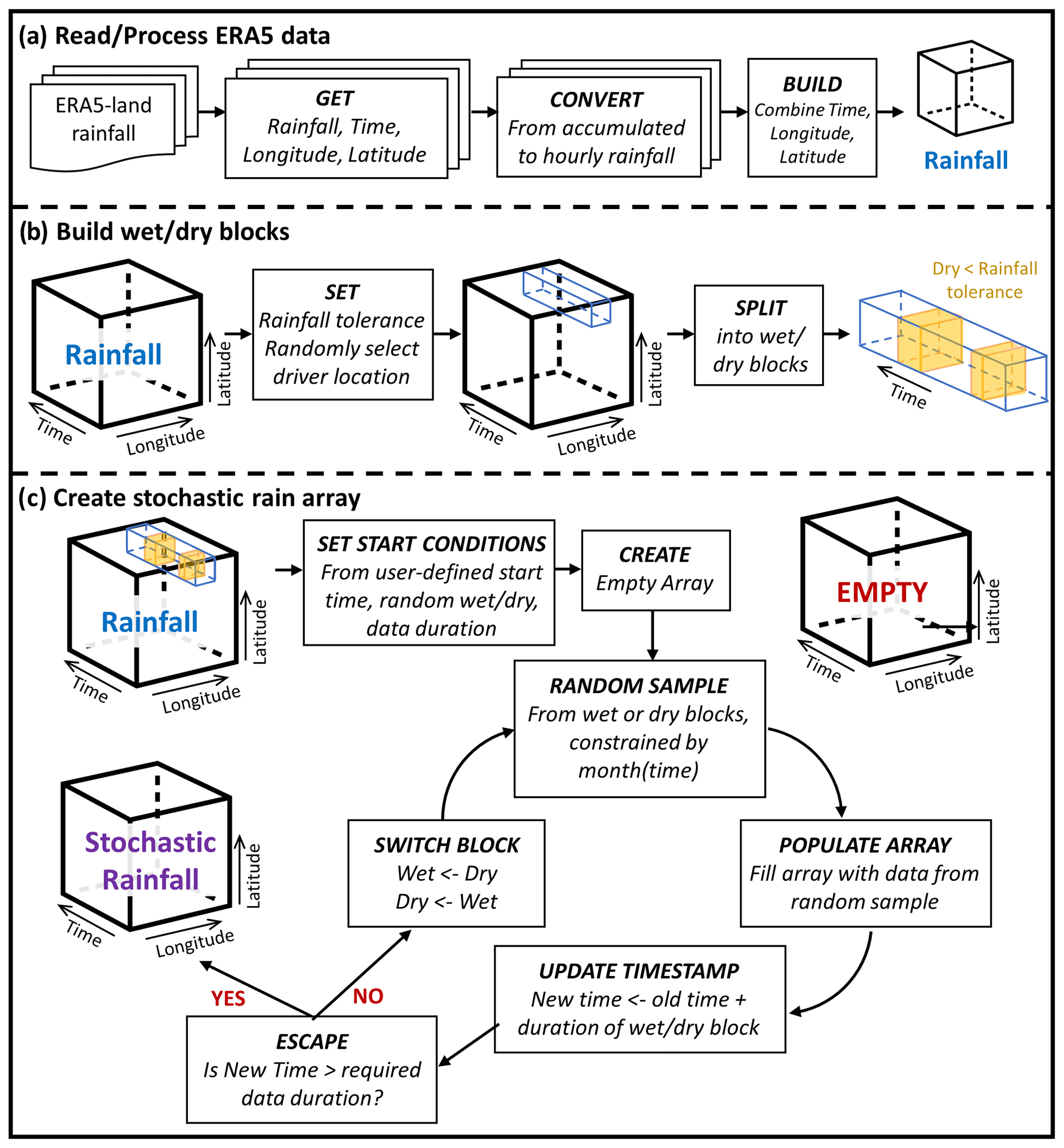
Figure 1SWM algorithm flow diagram: (a) read and process ERA5-Land data, (b) build wet and dry blocks, and (c) create stochastic array.
The Rangitāiki–Tarawera catchment is an area susceptible to many natural hazards including volcanic eruptions, flooding, and extreme weather events (ex-tropical cyclones). Hourly rainfall data across an 11 × 14 grid (Fig. 2) of longitude {176, 176.1, …, 177.0° E} and latitude {37.8, 37.9, …, 39.1° S} for 40 years (1981–2020) are downloaded from ERA5-Land. The ERA5-Land data are then prepared for the Rangitāiki–Tarawera catchment through SWM by converting these individual NetCDF files into an 11 (longitude steps of 0.1° E) by 14 (latitude steps of 0.1° S) by ∼ 350 400 (time steps in hours) array of hourly data (24 h × 365 d × 40 years). The Rangitāiki–Tarawera array is then split into wet/dry time-stamped blocks. ERA5-Land precipitation data at this catchment were commonly of very small (∼ 10−18 m) but non-zero values (common for ERA5-Land data; Muñoz-Sabater et al., 2021). The New Zealand climate report for the region (Chappell, 2013) provides average monthly rain and wet days at Kawerau (a town central to the catchment) of 112 per year (∼ 31 %), where wet days are defined as more than 1 mm d−1. A rainfall tolerance level of zero would result in ∼ 54 % of data being classified as wet, whereas using the climate report criterion (less than 1 mm rainfall in 24 h = 4.12 × 10⁻⁵ m h−1) resulted in ∼ 29 % of data defined as wet. For this exemplar, the latter quantity was used. Stochastic precipitation data for the Rangitāiki–Tarawera catchment were then built using SWM with a starting date of 1 January to obtain 999 sets of 40 years' worth of hourly stochastic rainfall data across the region as 999 NetCDF files. The number of runs (999) was chosen here to provide 95th-percentile bounds for the statistical analyses (Sect. 4), but in practice it can be set to any value, e.g. to match the number of downstream hazard simulations planned. This approach is common practice to assess statistical significance with non-parametric bootstrap methods (DiCiccio and Efron, 1996; Ramachandran and Tsokos, 2021).
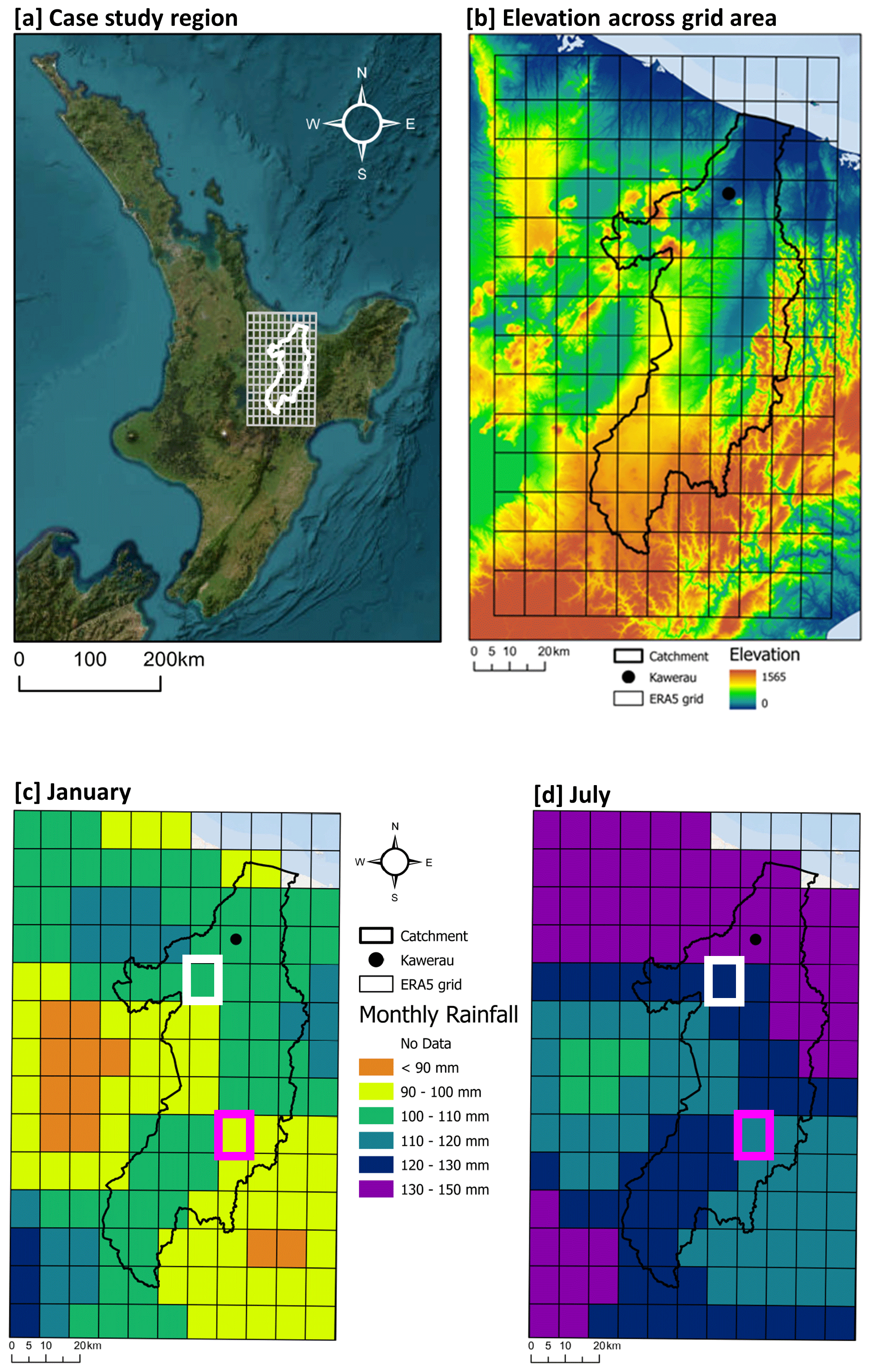
Figure 2ERA5-Land data across the case study area: (a) case study area, Te Ika-a-Māui / North Island, New Zealand, basemap from Earthstar Geographics (https://www.terracolor.net/, last access: 5 June 2024); (b) elevation of case study area with ERA5-Land grid, catchment of interest, and Kawerau township; (c) mean monthly total rainfall for January (ERA5-Land data: 1981 to 2020); (d) mean monthly total rainfall for July (ERA5-Land data: 1981 to 2020). Comparison locations in Fig. 3 are shown as white (Realisation 1) and pink (Realisation 2) boxes in (c) and (d).
Four sets of statistical analyses were undertaken to ensure that SWM-simulated data are stochastically similar to ERA5-Land data. For this, the 999 sets of 40 years of simulated data across the 11 × 14 grid are used, code for these analyses being in a GitHub repository and all outputs for the exemplar in the Supplement. The locations at which tests are performed were selected randomly, and the whole process was run through twice to check realisation sensitivity. The latter exercise was to check whether any patterns observed in the first 999 sets of simulated data were repeated in the second set. These are referred to as Realisation 1 and Realisation 2 in the results, with each realisation containing 999 sets of simulated data. The analyses were as follows.
-
Monthly means and variance.
Student's t test was used to compare the monthly mean rainfall between real and simulated data, and the Shapiro–Wilk test was used to test normality in order to select the appropriate equal variance test: Bartlett if data were normally distributed or Levene if not (Fox and Weisberg, 2019).
-
Significance of month and source for rainfall prediction.
Tukey's honest significant difference (HSD) (e.g. Miller, 1981) was used to determine whether source (real or simulated) is a significant factor in the prediction of total monthly rainfall.
-
Distributions of monthly rainfall totals.
A non-parametric bootstrap method was applied whereby empirical cumulative distribution functions (eCDFs) for each simulated dataset representing the 95th-percentile envelope (from 999 runs) are overlaid by the real dataset to determine if the latter is within the resulting envelope.
-
Temporal trends on daily and monthly timescales.
Autocorrelations are calculated for both the real and the simulated data to compare any significant lags (Venables and Ripley, 2002). Calculations require a continuous variable in discrete time, so they are run on cumulative daily and cumulative monthly rainfall timescales.
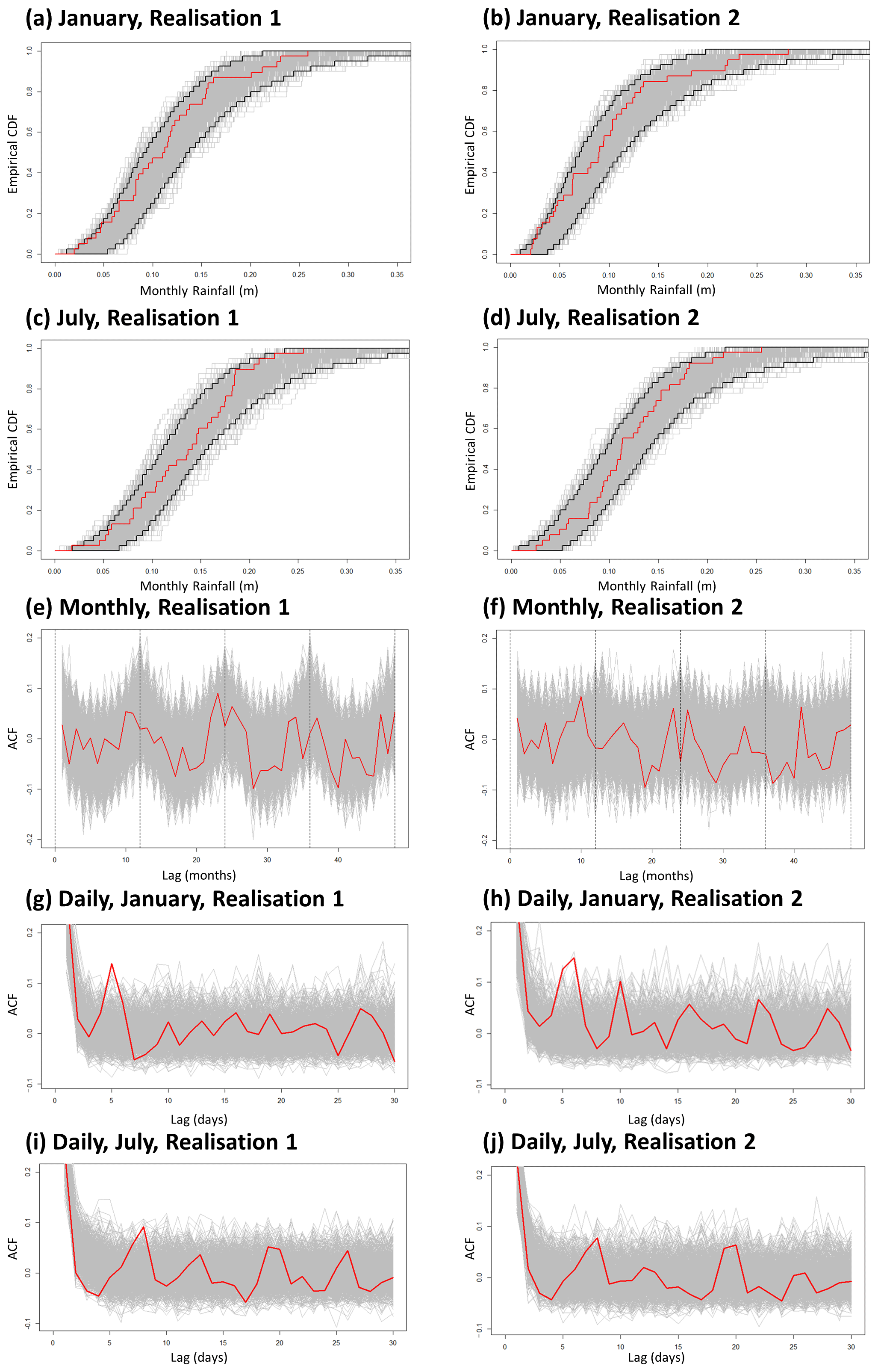
Figure 3Statistical analysis results. Simulated data are shown as grey lines, and real data are shown as red lines. (a) Realisation 1: January empirical cumulative distribution functions of rainfall totals (m); (b) Realisation 2: January empirical cumulative distribution functions of rainfall totals (m); (c) Realisation 1: July empirical cumulative distribution functions of rainfall totals (m); (d) Realisation 2: July empirical cumulative distribution functions of rainfall totals (m); (e) Realisation 1: monthly cumulative rainfall autocorrelations; (f) Realisation 2: monthly cumulative rainfall autocorrelations; (g) Realisation 1: January daily cumulative rainfall autocorrelations; (h) Realisation 2: January daily cumulative rainfall autocorrelations; (i) Realisation 1: July daily cumulative rainfall autocorrelations; (j) Realisation 2: July daily cumulative rainfall autocorrelations. The 95th-percentile bounds for (a) to (d) are represented by the black lines and are built from the 999 runs of simulated data (grey lines). Results are shown for a single randomly selected grid point; here results are shown at locations identified in Fig. 2.
Overall, while SWM passed all statistical tests for both realisations, some departure was noted in several combinations, the specifics of which are detailed below (see Supplement for a complete set of results).
-
Monthly means and variance.
Real data failed the Shapiro–Wilk test of normality (p=0.001), and realisations failed (p<0.05) for 41 % (Realisation 1) and 52 % (Realisation 2) of the 999 simulations respectively. Thus, the Levene test for equal variance was always used.
Realisation 1. Only 105 of 11 988 (12 × 40) tests showed a statistically significant difference (p<0.05) in monthly means compared to the real data, the expected number under the null hypothesis of no difference being 599 (11 988 × 0.05). A total of 679 pairs of real–simulated months (5.7 %) failed the test of equal variance (p<0.05), of which 410 were in May.
Realisation 2. Only 76 of 11 988 (12 × 40) tests showed a statistically significant difference in monthly means (p<0.05). A total of 445 pairs (3.8 %) failed the test of equal variance (p<0.05), of which 189 were in June and 63 in February.
-
Significance of month and source for rainfall prediction.
Two linear models were built with rainfall as the response variable and both month and source (real or simulated) as predictor variables. One was built with an interaction term (m1) and one without (m2). Both models for both realisations passed Tukey's HSD test, rejecting source as a statistically significant predictor (Realisation 1: p=0.987; Realisation 2: p=0.989).
-
Distribution of monthly rainfall totals.
Realisations 1 and 2. Envelopes were built for each realisation and for each month from eCDFs of the simulated data; these were then overlaid by the real data, which consistently fell within this 95th-percentile envelope (examples in Fig. 3a–d).
-
Temporal trends on daily and monthly timescales.
Realisations 1 and 2. Autocorrelations for cumulative daily rainfall for both real and simulated data over longer time lags (> 30 d) showed minimal trends through time. However, because we cannot reject a conclusion of similar trends between the two, results remain inconclusive. Looking within monthly data only and over shorter time lags (< 30 d), there are potential departures of the real data more positively correlated than the simulated data for January at a lag of 5 d (Fig. 3g–h) and for July at a lag of 8 d (Fig. 3i–j). Autocorrelations at the monthly scale show seasonal trends in both real and simulated data (Fig. 3e–f) with strong positive correlations at the yearly level (every 12 months) and negative correlations at the 6-monthly level (e.g. rainfall in January is negatively correlated with rainfall in July). A potential horizontal offset is noted between real and simulated data. The differences between real and simulated data here are attributed to multi-day rain or dry events. For example, in the simulated data, a large wet block representing a tropical cyclone in the original data occurring entirely in December can feasibly start on 31 December in the simulated data and thus will run over into January. January and July results are provided here as they represent not only the most extreme weather months for the region (in terms of both drought and heavy rainfall) but also the most extreme departures from the simulated data. The remainder of the months do not show any notable differences in lags between simulated and real data for either realisation (see the Supplement for the complete result set).
The method and code provided through this brief communication can be used to rapidly generate multiple sets of realistic, long-term, hourly precipitation data over a spatial region. While the outputs may not have the nuances that come with more complex models (e.g. Burton et al., 2008; Papalexiou, 2022), the efficient open-source code, written in an open-source language and based on open-source data, facilitates an easy-to-plug-in input for hazard simulations to support long-term, time and spatially varying, probabilistic risk assessments, uncertainty quantification, and multi-hazard models.
Code is written in R (open-source software) and is freely available at https://doi.org/10.5281/zenodo.11479909 (Whitehead, 2024).
All data were obtained from the Copernicus Climate Change Service (C3S) Climate Data Store (CDS), available here: https://doi.org/10.24381/cds.e2161bac (Muñoz Sabater, 2019). They are published under a Creative Commons Attribution 4.0 International (CC BY 4.0) licence.
The supplement related to this article is available online at: https://doi.org/10.5194/nhess-24-1929-2024-supplement.
Both authors conceptualised the model, MGW built the model, and statistical tests were guided by MSB and coded by MGW.
The contact author has declared that neither of the authors has any competing interests.
Publisher’s note: Copernicus Publications remains neutral with regard to jurisdictional claims made in the text, published maps, institutional affiliations, or any other geographical representation in this paper. While Copernicus Publications makes every effort to include appropriate place names, the final responsibility lies with the authors.
The two anonymous referees greatly improved this paper and especially breadth of tests detailed in the Supplement through their recommendations.
This research has been supported by the Resilience to Nature's Challenges Multi-hazard Risk model programme, New Zealand (grant no. GNS-RNC043).
This paper was edited by Dan Li and reviewed by two anonymous referees.
Arnaud, P., Bouvier, C., Cisneros, L., and Dominguez, R.: Influence of rainfall spatial variability on flood prediction, J. Hydrol., 260, 216–230, https://doi.org/10.1016/S0022-1694(01)00611-4, 2002.
Burton, A., Kilsby, C., Fowler, H., Cowpertwait, P., and O'Connell, P.: RainSim: A spatial–temporal stochastic rainfall modelling system, Environ. Modell. Softw., 23, 1356–1369, https://doi.org/10.1016/j.envsoft.2008.04.003, 2008.
Chappell, P. R.: The climate and weather of Bay of Plenty, 3rd edn., NIWA Science and Technology Series, Number 62, https://niwa.co.nz/static/BOP ClimateWEB.pdf (last access: 23 August 2023), 2013.
DiCiccio, T. and Efron, B.: Bootstrap Confidence Intervals, Stat. Sci., 11, 189–212, https://www.jstor.org/stable/2246110 (last access: 5 June 2024), 1996.
Fox, J. and Weisberg, S.: An R Companion to Applied Regression, 3rd edn., Sage Publications, Thousand Oaks CA, USA, 576 pp., https://socialsciences.mcmaster.ca/jfox/Books/Companion/ (last access: 5 June 2024), 2019.
Gao, L., Zhang, L., and Lu, M.: Characterizing the spatial variations and correlations of large rainstorms for landslide study, Hydrol. Earth Syst. Sci., 21, 4573–4589, https://doi.org/10.5194/hess-21-4573-2017, 2017.
Gill, J. C. and Malamud, B. D.: Hazard interactions and interaction networks (cascades) within multi-hazard methodologies, Earth Syst. Dynam., 7, 659–679, https://doi.org/10.5194/esd-7-659-2016, 2016.
Hyman, D. M., Bevilacqua, A., and Bursik, M. I.: Statistical theory of probabilistic hazard maps: a probability distribution for the hazard boundary location, Nat. Hazards Earth Syst. Sci., 19, 1347–1363, https://doi.org/10.5194/nhess-19-1347-2019, 2019.
Miller, R. G.: Normal Univariate Techniques, in: Simultaneous Statistical Inference, Springer Series in Statistics, Springer, New York, NY, 37–108, https://doi.org/10.1007/978-1-4613-8122-8_2, 1981.
Muñoz Sabater, J.: ERA5-Land hourly data from 1950 to present, Copernicus Climate Change Service (C3S) Climate Data Store (CDS) [data set], https://doi.org/10.24381/cds.e2161bac, 2019.
Muñoz-Sabater, J., Dutra, E., Agustí-Panareda, A., Albergel, C., Arduini, G., Balsamo, G., Boussetta, S., Choulga, M., Harrigan, S., Hersbach, H., Martens, B., Miralles, D. G., Piles, M., Rodríguez-Fernández, N. J., Zsoter, E., Buontempo, C., and Thépaut, J.-N.: ERA5-Land: a state-of-the-art global reanalysis dataset for land applications, Earth Syst. Sci. Data, 13, 4349–4383, https://doi.org/10.5194/essd-13-4349-2021, 2021.
Papalexiou, S.: Rainfall generation revisited: Introducing CoSMoS-2s and advancing copula-based intermittent time series modeling, Water Resour. Res., 58, 1–3, https://doi.org/10.1029/2021WR031641, 2022.
R Core Team: R: A language and environment for statistical computing, R Foundation for Statistical Computing, Vienna, Austria, R-project [code], https://www.R-project.org/ (last access: 5 June 2024), 2021.
Ramachandran, K. and Tsokos, C.: Mathematical Statistics with Applications in R, 3rd edn., Academic Press, Elsevier, https://doi.org/10.1016/B978-0-12-817815-7.01001-0, 2021.
Thompson, M. A., Lindsay, J. M., and Gaillard, J. C.: The influence of probabilistic volcanic hazard map properties on hazard communication, J. Appl. Volc., 4, 1–24, https://doi.org/10.1186/s13617-015-0023-0, 2015.
Venables, W. N. and Ripley, B. D.: Modern Applied Statistics with S, 4th edn., Springer Series in Statistics and Computing, Springer-Verlag, New York, NY, 498 pp., https://doi.org/10.1007/978-0-387-21706-2, 2002.
Whitehead, M.: MelWhitehead/SWM: SWM – Stochastic Weather Model in R, Zenodo [code], https://doi.org/10.5281/zenodo.11479909, 2024.
Wickham, H., François, R., Henry, L., Müller, K., and Vaughan, D.: dplyr: A Grammar of Data Manipulation, https://github.com/tidyverse/dplyr (last access: 5 June 2024), 2023.
Zhao, Y., Nearing, M. A., and Guertin, D. P.: A daily spatially explicit stochastic rainfall generator for a semi-arid climate, J. Hydrol., 574, 181–192, https://doi.org/10.1016/j.jhydrol.2019.04.006, 2019.
- Abstract
- Introduction
- Algorithm construction
- Example application: Rangitāiki–Tarawera catchment, Te Moana-a-Toi / Bay of Plenty, New Zealand
- Evaluation method
- Results
- Conclusions
- Code availability
- Data availability
- Author contributions
- Competing interests
- Disclaimer
- Acknowledgements
- Financial support
- Review statement
- References
- Supplement