the Creative Commons Attribution 4.0 License.
the Creative Commons Attribution 4.0 License.
 | 23 May 2024
Modelling seismic ground motion and its uncertainty in different tectonic contexts: challenges and application to the 2020 European Seismic Hazard Model (ESHM20)
Graeme Weatherill
Sreeram Reddy Kotha
Laurentiu Danciu
Susana Vilanova
Fabrice Cotton
Current practice in strong ground motion modelling for probabilistic seismic hazard analysis (PSHA) requires the identification and calibration of empirical models appropriate to the tectonic regimes within the region of application, along with quantification of both their aleatory and epistemic uncertainties. For the development of the 2020 European Seismic Hazard Model (ESHM20) a novel approach for ground motion characterisation was adopted based on the concept of a regionalised scaled-backbone model, wherein a single appropriate ground motion model (GMM) is identified for use in PSHA, to which adjustments or scaling factors are then applied to account for epistemic uncertainty in the underlying seismological properties of the region of interest. While the theory and development of the regionalised scaled-backbone GMM concept have been discussed in earlier publications, implementation in the final ESHM20 required further refinements to the shallow-seismicity GMM in three regions, which were undertaken considering new data and insights gained from the feedback provided by experts in several regions of Europe: France, Portugal and Iceland. Exploration of the geophysical characteristics of these regions and analysis of additional ground motion records prompted recalibrations of the GMM logic tree and/or modifications to the proposed regionalisation. These modifications illustrate how the ESHM20 GMM logic tree can still be refined and adapted to different regions based on new ground motion data and/or expert judgement, without diverging from the proposed regionalised scaled-backbone GMM framework.
In addition to the regions of crustal seismicity, the scaled-backbone approach needed to be adapted to earthquakes occurring in Europe's subduction zones and to the Vrancea deep seismogenic source region. Using a novel fuzzy methodology to classify earthquakes according to different seismic regimes within the subduction system, we compare ground motion records from non-crustal earthquakes to existing subduction GMMs and identify a suitable-backbone GMM for application to subduction and deep seismic sources in Europe. The observed ground motion records from moderate- and small-magnitude earthquakes allow us to calibrate the anelastic attenuation of the backbone GMM specifically for the eastern Mediterranean region. Epistemic uncertainty is then calibrated based on the global variability in source and attenuation characteristics of subduction GMMs.
With the ESHM20 now completed, we reflect on the lessons learned from implementing this new approach in regional-scale PSHA and highlight where we hope to see new developments and improvements to the characterisation of ground motion in future generations of the European Seismic Hazard Model.
- Article
(21863 KB) - Full-text XML
- BibTeX
- EndNote


In modern practice, PSHA formally incorporates both the aleatory variability inherent within the seismogenic source model and ground motion model, as well as the epistemic uncertainty associated with the choice and/or parameterisation of these respective models. The result is a suite of seismic hazard curves, each quantifying the probability of exceeding a given level of ground motion at a site (developed by integrating over all the probability distributions represented by the aleatory uncertainty) and collectively describing the distribution of probabilities of exceedance for each given level of ground motion that reflects our current knowledge of the earthquake system for the region in question. Probabilistic seismic hazard curves yield a wide array of products that are useful for many stakeholders, including hazard maps of ground motions with fixed probabilities of exceedance that can form inputs to zonations adopted within seismic design codes, as well as uniform hazard spectra that describe an acceleration spectrum with constant probability of exceedance across a range of periods. The probabilistic seismic hazard models can also be combined with data describing the number and geographical distribution of buildings across a region, their typology and economic value, or the number of occupants within buildings in a given time of day (exposure), alongside probability distributions describing the likelihood of these buildings exceeding given degrees of damage (fragility) and economic or human loss (vulnerability) when subject to given levels of shaking. This latter process forms probabilistic seismic risk analysis, which yields products such as the expected average annual economic loss or fatalities (AAL) in a location or region, as well as loss curves that describe the probability of exceeding given levels of loss within a specified time period.
Probabilistic seismic hazard and risk models can now be found for every country in the world (Pagani et al., 2020; Silva et al., 2020), and within the last 2 to 3 decades several regions have developed successive generations of earthquake hazard and risk models, each building upon lessons learned, new developments and new data gathered since the last model. Europe is one such region, boasting a varied suite of national-scale earthquake hazard and risk models within its constituent countries, as well as a state of the art, open and transparent pan-European analysis in the form of the 2013 European Seismic Hazard Model (ESHM13) (Woessner et al., 2015). Following the publication of ESHM13, insights from subsequent national-scale analysis, alongside expansion of earthquake data across Europe, prompted the development of a new seismic hazard model and, for the first time, an open and reproducible seismic risk model for Europe. These are the 2020 European Seismic Hazard Model (Danciu et el., 2021) and the 2020 European Seismic Risk Model (Crowley et al., 2021), which we will refer to as ESHM20 and ESRM20 respectively.
The characterisation of expected ground motion and its aleatory variability was one of the critical areas for update and revision in the ESHM20 and ESRM20. Both specified their own needs from the ground motion models (GMMs). The ESHM20 aimed to characterise seismic hazard on reference rock (Eurocode 8 soil class A, VS30 800 m s−1) across Europe, while ESRM20 also needed to consider local site amplification effects to characterise the levels of shaking to which the buildings in the exposure models may be subject. Additionally, both the ESHM20 and ESRM20 aimed to quantify the epistemic uncertainty in hazard and losses, making this a crucial focal point for the GMM development.
In setting out to undertake this update to the European GMMs we had several overarching objectives. Firstly, we wanted to capitalise on the expanded data set of ground motions for Europe made available via the Engineering Strong Motion database (Luzi et al., 2020) and corresponding harmonised flatfile (Lanzano et al., 2019). From these data we aimed to refine the regionalisation of ground motion from its larger-scale divisions by tectonic region class (e.g., active shallow seismicity, stable cratons, subduction zones and non-subduction deep seismicity) to identify and integrate changes in ground motion over local scales and to allow the epistemic uncertainty to reflect the degree of information available from region to region. Finally, we aimed to take into account feedback and insights into ground motion modelling and its uncertainty that emerged from national-scale PSHA models since ESHM13. The outcomes of several years' work were a set of GMMs and their corresponding epistemic uncertainties developed for application to PSHA in Europe, which represented a paradigmatic change from previous approaches by building upon the concept of a regionalised scaled-backbone logic tree. This approach was then adapted to different tectonic environments across Europe, reflecting different degrees of knowledge or volumes of data. These included active regions of shallow seismicity; stable cratonic regions of low seismicity; subduction zones in the Hellenic, Cypriot and Calabrian arcs; and the complex, yet hazardous, Vrancea deep seismogenic zone.
The work to develop the ground motion model logic tree for ESHM20 and ESRM20, as well as all its constituent components, has been so extensive that it is disseminated across several connected publications. The core (backbone) ground motion model for application to shallow seismicity in Europe was developed by Kotha et al. (2020) and subsequently updated following feedback and further analysis into large-magnitude scaling of ground motion by Kotha et al. (2022). The adaptation of this model into the regionalised scaled-backbone GMM logic tree framework is described in Weatherill et al. (2020), while the approach taken to apply it to the special case cratonic region of northeastern Europe is explained in Weatherill and Cotton (2020). With the ESRM20 requirement of characterising ground motion on the soil surface across all regions of building exposure in Europe, a novel approach was needed to represent the local-scale site amplification in the seismic risk calculations and to propagate the increased uncertainties from the regional-scale approach into the probabilistic assessments of loss. This is explained in detail by Weatherill et al. (2023), and the way the site model is calibrated to represent the most suitable input for the given exposure model is described by Dabbeek et al. (2021). In addition, a brief overview of the whole model can be found in the technical reports released with the ESHM20 (Danciu et al., 2021) and ESRM20 (Crowley et al., 2021).
Despite multiple publications on this topic, not every part of the ESHM20 GMM logic tree is fully described in the scientific literature. Two areas require further attention, and the aim of the current paper is to present these with a complete discussion of the rationale and analysis that underpinned their development. The first of these two areas is the discussion of the special case regions. Following completion and implementation of the logic tree in the first iteration on PSHA for Europe, we received feedback from scientists across different areas of Europe who highlighted where refinements could be made, mostly based on additional or new data not used in the compilation of the Engineering Strong Motion (ESM) database. These include France, Portugal and Iceland, where we undertook further analysis that prompted us to adjust the current models to reflect the insights gained from these additional data. The second of the two areas is the GMM for subduction and deep seismicity. Here the scaled-backbone GMM was developed using a different approach from that presented in Weatherill et al. (2020) and Weatherill and Cotton (2020), which brought its own challenges in trying to transform insights from available data and from developments in subduction ground motion modelling. The current paper is divided into four main sections. In Sect. 2, we present an overview of the regionalised scaled-backbone logic tree for shallow seismicity (both stable non-craton and stable craton), including its rationale, development and insights from the initial hazard applications. In Sect. 3 we will focus on the special cases, explaining what prompted further consideration and how we used insights from other models and data to adapt the GMM logic tree in the final ESHM20 and ESRM20. Section 4 presents a comprehensive overview of the subduction scaled-backbone logic tree, covering the classification of subduction ground motions from the ESM data set, the identification and calibration of the scaled-backbone model, and the subsequent adjustments that were needed to improve the application of the models in the PSHA calculations. Finally, we finish the paper in Sect. 5 with a discussion reflecting upon the development of the GMM logic tree, its advantages and limitations, the adaptability of the framework to future models of seismic hazards, and the insights gained from the work that will begin to form the areas of research focus for the next generation(s) of European seismic hazard and risk models. All of the ground motion models described in this publication are available in the OpenQuake software for seismic hazard and risk calculation (http://github.com/gem/oq-engine, last access: May 2024; Pagani et al., 2014) and can be explored by the eGSIM interactive web service for GMMs (https://egsim.gfz-potsdam.de/home, last access: May 2024); however, to facilitate their adoption in other applications we have also provided open-source implementations of the GMMs in the Python language in a stand-alone software repository (https://gitlab.seismo.ethz.ch/efehr/eshm20_gmms, last access: May 2024).
2.1 Background and motivation
The path toward updating the GMM logic tree for ESHM20 began in several preliminary studies that were undertaken early in the SERA project (circa 2017–2018). Shortly following the completion of the ESHM13 a new generation of ground motion models emerged, including those from the NGA West 2 project (Abrahamson et al., 2014; Boore et al., 2014; Campbell and Bozorgnia, 2014; Chiou and Youngs, 2014) and the European RESORCE project (Akkar et al., 2014a, b; Bindi et al., 2014; Derras et al., 2014) alongside new GMMs that update those that had been selected in ESHM13 (e.g., Pezeshk et al., 2011; Cauzzi et al., 2015; Abrahamson et al., 2016; Zhao et al., 2016a, b, c). In light of this, and with a focus on constraining broadband seismic hazards in Europe, Weatherill and Danciu (2018) undertook an interim update to the GMM selection for Europe, updating existing GMMs where possible and adding in new models to better capture epistemic uncertainty for parts of the logic tree where available models had been previously limited. Their results suggested a trend toward lower hazard across much of Europe particularly at short periods (with some notable exceptions such as Romania) and demonstrated that the new generations of models were capable of defining seismic hazard over a much more extended range of spectral periods.
After the completion of this study the new Engineering Strong Motion (ESM) database and corresponding flatfile were published (Lanzano et al., 2019; Bindi et al. 2019), which allowed us to apply the GMM log-likelihood scoring to the new generation of models using a vastly expanded set of ground motion records (Weatherill et al., 2018). This revealed that when evaluated at a European scale the newer models provided improved fits to data compared to those selected by ESHM13. However, the volume of observations available within ESM was such that country-to-country differences in the model-to-data fits could be observed within areas that had been previously classified uniformly as active shallow-crustal-seismicity regions. Such differences had been observed in recent GMM studies for Europe including Kale et al. (2015), Kotha et al. (2016) and Kuehn and Scherbaum (2016). While ESHM13 had broadly mapped Europe into seven tectonic categories (active shallow crust, stable shallow crust, shield, subduction interface, subduction in-slab, non-subduction deep and volcanic), further geographical variation in ground motion scaling within these domains was evident.
While analysis of the ESM records raised important questions about regionalisation of ground motion, changes in perspectives in the characterisation of epistemic uncertainty in ground motion models within the seismic hazard community prompted us to reconsider the general approach we had been adopting in the logic tree. Ground motion model epistemic uncertainty has been a key topic in the development of PSHA over several decades, and a substantial change in approach became more widespread in site-specific hazard analysis after ESHM13. Taken as a starting point, the study of Delavaud et al. (2012) presented a more formalised approach to the common practice of identifying and selecting multiple ground motion models from the scientific literature and implementing them in a logic tree framework with their corresponding weights (a multi-model or weights-on-models approach). The formalisation emerged from a dual process of pre-selection and expert judgement weighting of models, combined with data-driven testing using likelihood analysis (e.g., Scherbaum et al., 2009) to refine the model selection and define the weights. The process outlined by Delavaud et al. (2012) has been adopted and refined in other national PSHA models that followed the development of ESHM13 (e.g., Lanzano et al., 2020). Since then, however, the limitations of the multi-model approach for GMM logic tree development have been widely discussed in the PSHA community (e.g., Bommer, 2012; Atkinson et al., 2014; Bommer et al., 2015). Among them are the potential lack of available models in regions where data are limited (and thus uncertainty should be highest), inconsistencies in selection and/or definition of explanatory variables, and significant overlap in data used to fit the models resulting in convergence of multiple models toward the same values in the centre of the data set rather than capturing the body and range. More recent PSHA applications have instead proposed the adoption of the backbone approach, one in which a suitable model or set of suitable models is selected (the backbone(s)) and to which additional adjustments and their respective weights are applied to represent our epistemic uncertainty in source, attenuation and site characteristics for our target region in question and mapped into the logic tree, hence becoming a scaled-backbone ground motion logic tree.
The scaled-backbone logic tree changes our approach to epistemic uncertainty characterisation by moving the question away from one of identifying which models and how many would be needed to represent the centre, body and range of technically defensible interpretations of the data to one of how do we select a suitable model and define adjustments to it in order to capture our uncertainty in the seismological properties of a region that influence ground motion. Bommer and Stafford (2020) present clearly how to address the selection of the backbone model, while definition, calibration and weighting of adjustment factors have been discussed in detail by Goulet et al. (2017) and Douglas (2018), among others. We should also note that the multi-model and scaled-backbone approaches do not necessarily need to be dichotomous, and there are many examples in recent PSHA studies that have selected multiple models as a basis for capturing region-to-region variability or epistemic uncertainty in functional form before applying additional scaling factors to the set of selected models to represent uncertainty in the seismological properties of the target region (e.g., Bommer et al., 2015; Grünthal et al., 2018; Bradley et al., 2023).
An early conceptual proposal for a backbone GMM logic tree that could be applied to PSHA in Europe was outlined by Douglas (2018). Though we adapt this concept for each of the different backbone GMM logic trees we built, the general principle expressed in this formulation remains. In his illustrative example, Douglas (2018) starts by using the GMM of Kotha et al. (2016) as the backbone model. This GMM is selected here because it is a regionalised GMM that calibrates different anelastic attenuation coefficients for Italy, Türkiye, and other regions, and this region-to-region variability is mapped into three equally weighted branches. Next Douglas (2018) looks at the distribution of ground motion residuals for different regions, focusing on magnitudes and distances in the well-constrained part of the data set used for the original model ( and ). The differences in residual distributions constrain an adjustment factor analogous to region-to-region variability in the source parameter (usually attributed to stress drop) and are then mapped into a second branch set containing three branches. Finally, the statistical uncertainty of the model (σstatistical) is constrained from the confidence limits of the regression based on a finite data set (Al Atik and Youngs, 2014). This distribution is Gaussian and is mapped into three branches corresponding to the 5th, 50th and 95th percentile of the distribution.
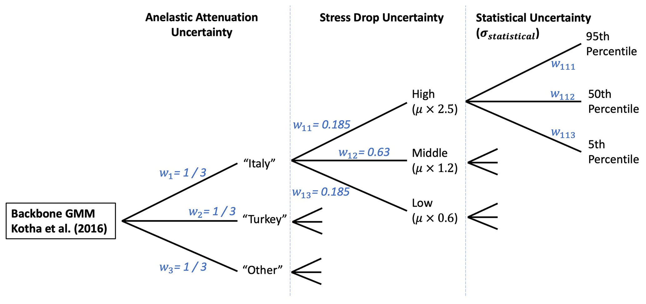
Figure 1Conceptual framework for a scaled-backbone GMM logic tree proposed by Douglas (2018).
The proposed backbone model, illustrated in Fig. 1, contains 27 branches and is primarily using region-to-region variability implied in the data to define a maximum uncertainty, which would apply in regions where few data are available. However, this same framework can be adjusted to data-rich regions, where the observed strong motions allow for calibration of the anelastic attenuation and stress drop uncertainty distributions to centre on the trends implied from local data and with the resulting width of the uncertainty distribution reducing accordingly. Using this concept, we arrive at a regionalised scaled-backbone GMM logic tree – one in which a best suited model is selected for application – but the region-to-region variability informs the scaling and weights of the logic tree branches. The rest of this section will focus on how this framework was applied in practice to shallow seismicity in active and non-cratonic stable regions as well as to cratonic stable regions. We will also outline some of the lessons learned in constructing the model and applying it in practice.
2.2 Development of the GMM logic tree for shallow crustal seismicity (non-craton)
The ESM database and associated flatfile (Lanzano et al., 2019) provides more than 20 000 strong-motion observations from across Europe, with Italy, Türkiye, Switzerland, Greece and Romania especially well represented. For the selection of the backbone GMM we opted to derive a new model for Europe that capitalises on these data, which was published in Kotha et al. (2020). Shallow seismicity is defined for the current purpose according to the criteria adopted by Kotha et al. (2020) – namely that the event has a depth less than 39 km, located in regions for which the Moho depth is between 14 and 49 km. A further criterion is added to exclude shallow earthquakes associated with the subduction system, which were classified using the fuzzy classification system described in Sect. 4 of this paper. In their earlier work, Kotha et al. (2016) had identified regional variations in ground motion model scaling for Europe and with the vastly expanded data set provided by the ESM. The basic functional form of the model by Kotha et al. (2020) is described by
where Y is the intensity measure of interest (e.g., PGA, PGV and/or Sa (T)), Mw is the moment magnitude of the earthquake, RJB is the Joyner–Boore distance and h is the hypocentral depth. The magnitude scaling term fM(Mw) is described by
Mh represents the hinge magnitude for upper magnitude scaling, which was originally fixed to Mw 6.2 in Kotha et al. (2020) but later revised to Mw 5.7 in Kotha et al. (2022), which will be discussed in due course.
The distance scaling is described by both its geometric spreading (fR,g) and apparent anelastic attenuation (fR,a) components:
where hD(h) is the effective depth, which takes the values of 4, 8 and 12 km for hypocentral depths h in the ranges h≤10 km, km and h > 20 km respectively. e1, b1−b3 and c1−c3 are period-dependent coefficients, while Mref and Rref are period-independent reference magnitude and distance, fixed to Mw 4.5 and RJB= 30 km respectively. The remaining terms in the model are period-dependent random effects determined by mixed-effects regression, with δL2Ll representing the region-specific source parameter, the region-corrected between-event residual, δS2SS the site-to-site residual, δc3,r the region-specific apparent anelastic attenuation parameter (residual attenuation), and the δW0 the event- and site-corrected residual. Each of these residual terms is normally distributed such that , , , and . Three of these terms (, δS2Ss and δW0) are dependent on the event e and site s, while δL2Ll and δc3,r are region dependent. For these region-dependent properties, rather than divide the data set by country we adopted two prior regionalisations that are based on tectonics and geology. The first is the TECTO zonation, used in the construction of the ESHM20 seismogenic source model, and the second is a geology-based regionalisation proposed by Basili et al. (2021) as part of the Probabilistic earthquake-induced Tsunami Hazard Assessment for the coastlines of the Northeast Atlantic and the Mediterranean (TSUMAPS-NEAM). In undertaking the regressions, the δL2Ll is dependent on the TECTO zone in which the earthquake source occurs, while δc3,r depends on the zone from the Basili et al. (2021) regionalisation in which the recording station is situated. The variation in these two terms across their respective regions is shown for a spectral period of T= 0.1 s in Fig. 2.
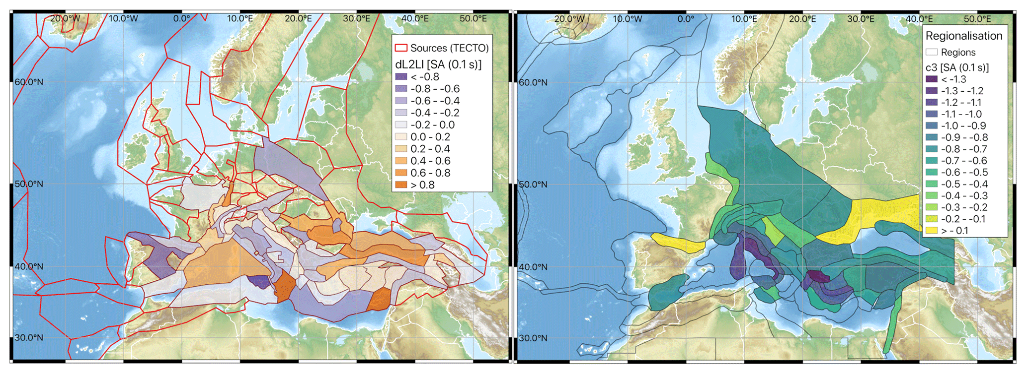
Figure 2Regional variation in δL2Ll (left) and (right) for Sa (0.1 s) using the TECTO and Basili et al. (2021) regionalisations respectively (Figures reproduced from Weatherill et al., 2020).
2.2.1 Regionalising the scaled-backbone GMM logic tree
The random effects δL2Ll and δc3,r allow us to describe the region-to-region variation in source parameter scaling (a measure of how much more or less energetic earthquakes may be in each region) and residual attenuation (a measure of the extent to which ground motion decays more or less rapidly in a region). While each effect may change the ground motion prediction in a locality, their standard deviations τL2L and τc3 are quantitative estimations of the total region-to-region variability implied by the underlying data set. This can be mapped directly into the scaled-backbone framework proposed by Douglas (2018), in which the first two branch sets describe the uncertainty in attenuation and in the stress drop respectively. Scaling factors and weights emerge naturally from the fact that the epistemic uncertainty is being described by Gaussian distributions, which we approximate with NBR discrete branches using the Gaussian quadrature approach of Miller and Rice (1983).
Using N(0,τL2L) and N(0,τc3) to describe epistemic uncertainty in the median ground motion requires an important assumption, which is that the seismological properties of the target region are represented within the data set used to calibrate the distributions. Specifically in this case, do we believe that among the regions for which we have calculated δL2Ll and δc3,r using the ESM data set some may be consistent with the seismological properties of regions for which we do not have data? With few or no available records in a target region, this may need to be inferred from other information, which we will consider in further detail for the case of the craton region. Where we do believe that the seismological properties of the host region are consistent with or representative of those of the target region, but cannot calibrate region-specific distributions of δL2Ll and δc3,r, we apply the full distributions of N(0,τL2L) and N(0,τc3) respectively. We refer to this as the “default” scaled-backbone model, and we apply it predominantly in non-cratonic regions of low-to-moderate seismicity and/or regions of higher seismicity where data are limited or absent from ESM.
The default scaled-backbone model reflects the maximum region-to-region variability inferred from our data, but for regions that are well sampled by the ESM data set and for which we have reasonably well-calibrated δL2Ll and δc3, we can integrate this information into the logic tree. This allows us to tune the GMM logic tree to the seismological properties inferred by the data in the region, and in doing so reducing the epistemic uncertainty with respect to that of the default backbone. In effect, we are seeking to constrain and for all R (where R includes one or more regions of the underlying regionalisations) for which we have data, assuming that both and . This process cannot necessarily be undertaken blindly, however, and in deciding how to allow the data to refine the model we took into consideration several factors: the degree of confidence we may have in the calibrated random effects (i.e., how many observations were available in each region), potential sources of bias in the observations that may be used to constrain a random effect, and the consistency of observations with both our fundamental understanding of the earthquake process in a region and/or previous studies and observations in those same regions. For δL2Ll, the tectonic locality-to-locality (l) variability, a limiting factor is that in many tectonic localities either there are still very few earthquakes from which this can be constrained reliably or the earthquakes that are present come from a single seismic sequence and may thus be representative of the temporally dependent properties of that sequence rather than of the region as a whole. After interpreting results such as those shown in Fig. 2 and exploring for dependencies of δL2Ll on factors such as style of faulting, a decision was taken not to attempt to regionalise δL2Ll on the basis of the data available but rather to assign N(0,τL2L) to all of the non-craton crustal seismicity regions. This may be a conservative assumption in certain regions contributing many earthquakes to the ESM database, such as central Italy, but it reflects our current degree of confidence. Naturally, we hope that with the addition of further earthquakes to the database it will be possible to refine this term to a greater extent in future models.
For the residual-attenuation term, δc3,r being based on the number of stations available in a region and indicative more of the local path and site properties, we had a greater degree of confidence in the regional trends that were emerging. The trends toward fast attenuation in central and southern Italy and in central Greece, as well as toward slower anelastic attenuation in northern and central Europe, are consistent with previous studies (e.g., Kotha et al., 2016; Kuehn and Scherbaum, 2016) and with other known geophysical properties such as the influence of volcanism, geological age and Moho depth. However, while the broad scale trends are well supported, we were cautious to suggest calibrating the logic tree to each of the 45 out of 105 regions in the Basili et al. (2021) regionalisation for which δc3,r was determined. This not only risked over-fitting the attenuation term of the logic tree, but in many cases the confidence intervals on δc3,r were especially large. Instead, when looking at the trends in δc3,r with a period, we could identify groups of regions that shared similar properties. We therefore applied hierarchical clustering to the vectors of δc3,r(T) for periods in the range 0.01 to 8 s, and from this we identified five clusters (hereafter caller cluster regions) that captured well the main regional trends. Within each cluster we used Bayesian fitting to retrieve , where is the mean and τc3,cl the standard deviation of the attenuation terms δc3,r for all regions contained within each cluster. Bayesian estimation minimises the possibility of over-fitting in the clusters to which few regions belong, ensuring that in these cases τc3,cl tends towards τc3. Together with the default scaled-backbone GMM logic tree, the five cluster-region-specific adjustments to the scaled-backbone model form the regionalised scaled-backbone logic tree and, as for the tectonic-location uncertainty distribution, can be approximated into NBR discrete branches according to Miller and Rice (1983). The distribution of expected ground motions from the logic tree is shown in Fig. 3 in terms of its attenuation with distance and variation with period.
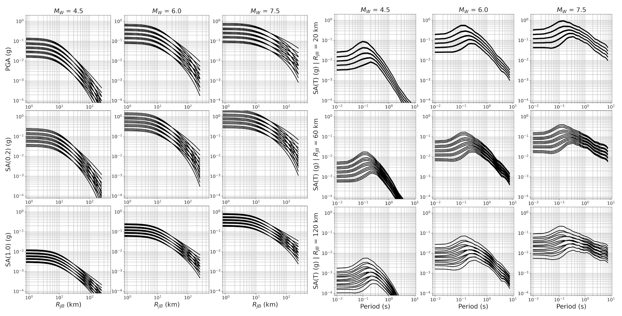
Figure 3Expected ground motion from all 15 branches of the default backbone GMM logic tree for shallow seismicity shown in terms of attenuation with distance (left image) and scaling with spectral period (right image). Columns refer to Mw 4.5, 6.0 and 7.5 respectively, while rows refer to intensity measures PGA, Sa (0.2 s) and Sa (1.0 s) for attenuation, or to distances of RJB 20, 60 or 120 km for Sa (T).
The third branch set of the scaled-backbone logic tree formulation proposed by Douglas (2018) refers to statistical uncertainty, or within-model uncertainty, σstatistical. This reflects the uncertainty resulting directly from the regression of the model on the data set, which is calculated here for each scenario () using the method of Al Atik and Youngs (2014). σstatistical is a measure of the degree of confidence in the model and should be smaller in the range of the scenarios well constrained by the data and larger toward the extremes where fewer records are available to constrain the regression, such as large magnitudes and short distances. This term was calculated for the Kotha et al. (2020) GMM and was initially added to the logic tree, but after further consideration it was recognised that the statistical uncertainty is, to a large extent, contained within the region-to-region variability modelled in the other branch sets. Adding on additional branches for σstatistical would likely be double counting epistemic uncertainty for scenarios well constrained by the data, in which region-to-region variability is dominant. Comparing σstatistical against τc3 and τL2L, we found that the latter exceed the former across all scenarios except for those of large magnitudes and short distances. We therefore selected a compromise solution in which the tectonic-locality branches are represented by rather than τL2L. This ensured that where the model is well constrained, this term represents the region-to-region variability, while for poorly constrained scenarios it is the statistical uncertainty that dominates.
The complete logic tree representing the regionalised scaled-backbone GMM for application to non-cratonic shallow seismicity is shown in Fig. 4. In contrast to the formulation of Douglas (2018) the model now contains two branch sets, one describing the combined tectonic-locality variability and statistical uncertainty (N), which is not regionalised, and the second set representing residual-attenuation variability which is regionalised into a default region, N(c3,τc3), and five clusters each represented by their own cluster-region-specific distribution, . The spatial extents of the zones where either the default or a specific cluster-region distribution applies are also shown in Fig. 5. Further insights were gained when applying this model, which will be discussed in due course.
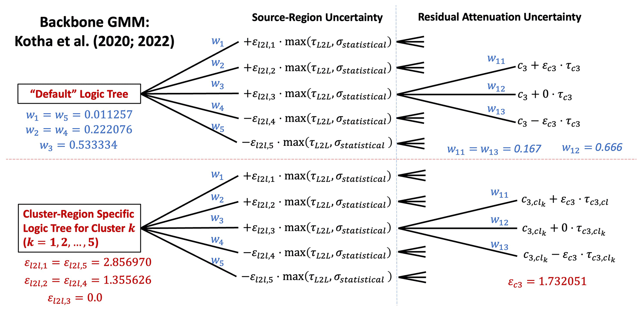
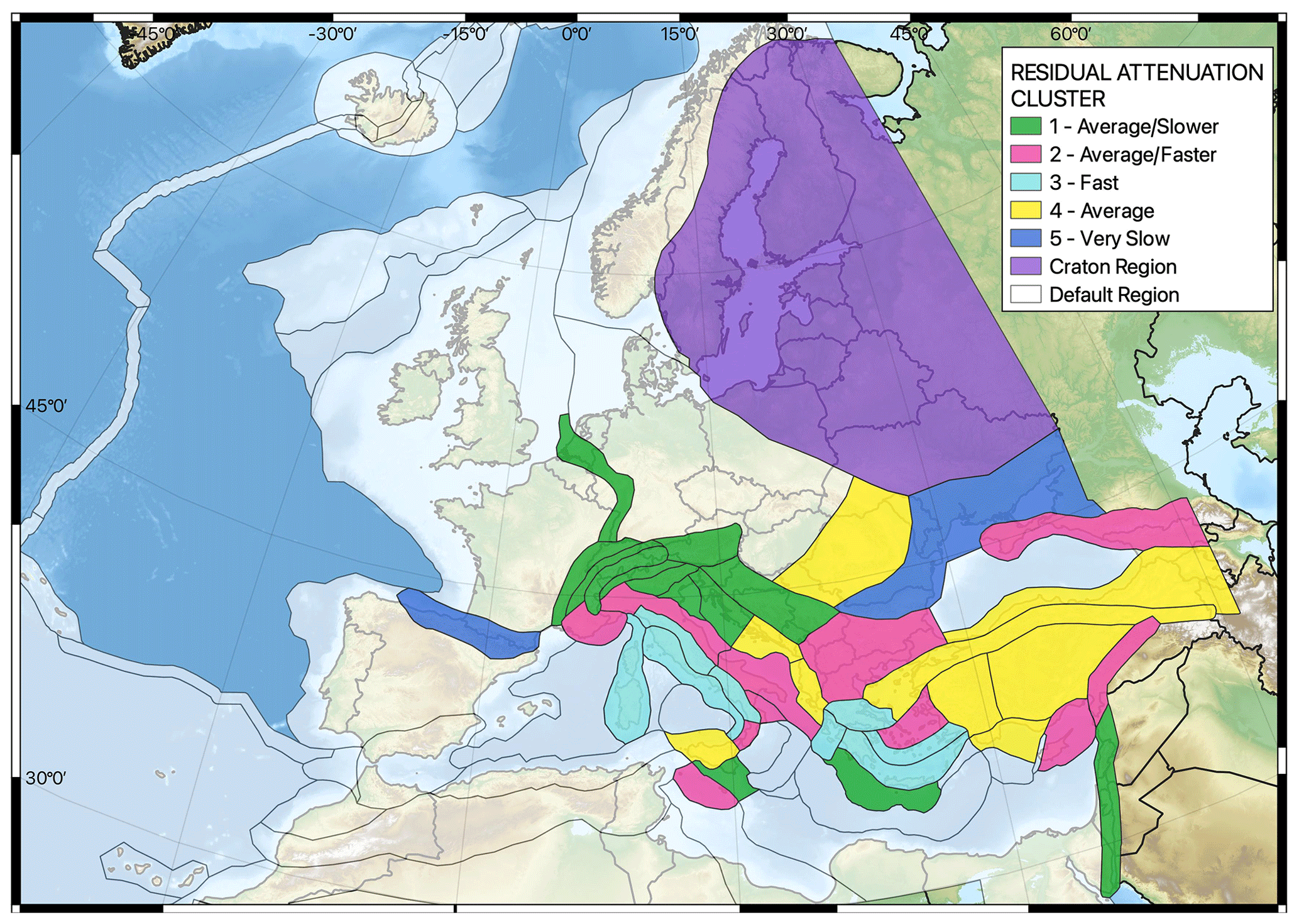
Figure 5Regionalisation and distribution of cluster regions adopted for the original proposal of the ESHM20 GMM logic tree for shallow seismicity (adapted from Weatherill et al., 2020).
2.3 GMM logic tree for seismicity in the cratonic region
Arguably one of the most critical assumptions that was made in defining and applying the shallow-crustal-seismicity scaled-backbone GMM logic tree was that the tectonic-locality and residual-attenuation region adjustment required for the target falls within the distributions described by N(0,τL2L) and N(0,τc3). Since these distributions are calibrated on ground motions recorded in predominantly southern and eastern Europe, can we know whether they can be applied throughout Europe even where recorded motions are limited or absent? To address this question Weatherill and Cotton (2020) consulted several different regional-scale data sets of geophysical properties that are likely to have an impact on source scaling and attenuation in order to identify clear and consistent regional-scale differences in crustal characteristics. These included a 1 s attenuation quality factor (QLG) (Mitchell et al. 2008), mantle shear wave velocity anomaly at 175 km depth (e.g., Mooney et al., 2012), heat flow (Lucazeau, 2019), Moho depth (Grad et al., 2009) and bedrock geology (Asch, 2005). All the data presented a clear and consistent contrast between northeastern Europe (i.e., the Baltic Sea and surrounding countries) and the rest of Europe. This delineates unambiguously the stable cratonic region of Europe, which is characterised by an older, colder and thicker continental crust than the rest of Europe. The transition occurs across the Trans-European Suture Zone (TESZ) that broadly extends from Denmark to the north coast of the Black Sea. The extent of the craton region is shown in Fig. 5.
The cratonic shield of Europe is well known to geologists and seismologists and has been treated separately in terms of ground motion attenuation in many previous generations of seismic hazard models, including the ESHM13. Extending comparisons of these same geophysical data sets globally, however, we could see clearly that the continental crust of the central and eastern United States (CEUS) and Canada is a closer analogue to that of the Baltic Shield than even the more tectonically stable regions of western Europe. This analogy is critical as it allows us to adopt developments from the recent Next Generation Attenuation models of the eastern US (NGA East, Goulet et al., 2017) to help construct a scaled-backbone GMM logic tree for application to the cratonic region of Europe. The use of the NGA East GMMs for this purpose should not necessarily be seen as a significant divergence from the regionalised backbone GMM strategy, but rather that we are utilising the distribution of predicted ground motions from the NGA East models as a proxy for regional data that is otherwise absent or limited to very small magnitudes in the case of Fülöp et al. (2020).
The NGA East project covered many different aspects of ground motion modelling in the CEUS, and several of these developments have been adopted directly or indirectly for the craton GMM logic tree here. The starting point is the suite of 20 GMMs developed for the very hard bedrock site conditions (VS=3000 m s−1) in the eastern United States by several teams. Each team used different methods for developing the model and making different assumptions about the source and path properties of the crust. Also added to this was an earlier model of Pezeshk et al. (2011), which was compatible with the approaches and assumptions of the NGA East models. For each magnitude (Mw) and source-rupture-to-site distance (RRUP) the distribution of expected ground motion from the 21 models forms a parametric measure of the model-to-model variability. This could be used directly as a non-parametric GMM, in which the epistemic uncertainty is scenario-dependent and could be mapped into a logic tree by , where εμ is the number of standard deviation above or below the median and is discretised using the same approach of Miller and Rice (1983) that we have seen for other distributions. As the aim is to use the NGA East data to regionalise the backbone model, Weatherill and Cotton (2020) instead fit a parametric GMM to the distribution of expected ground motion values, based on the functional form of Kotha et al. (2020) but with minor adjustments to accommodate the use of RRUP rather than RJB as the distance metric:
The functional forms of fM, fR,g and fR,a are the same as those described in Eqs. (2)–(4); however, with RRUP as the distance metric, hD is fixed to 5 km and Rref to 1 km. As with Kotha et al. (2020), robust regression is used to downweigh the influence of outliers on the coefficients of the model. The standard deviation σμ describes the total model-to-model variability in expected ground motion, which we can then map into NBR logic tree branches using Miller and Rice (1983). The aleatory uncertainty of the model is taken directly from the proposed aleatory uncertainty model for NGA East GMMs by Al Atik (2015), wherein their global heteroskedastic between- and single-station within-event uncertainty model is selected. More details are provided in Weatherill and Cotton (2020)
The parametric GMM in the form presented in Eq. (5) describes only the median ground motion on very hard rock (VS 3000 m s−1) but not the reference rock condition required for ESHM20. For this it was necessary to incorporate the linear and nonlinear amplification models of Stewart et al. (2020) and Hashash et al. (2020), which were developed for application in the CEUS as part of the NGA East project. The complete site amplification model comprises three components: F760(T), a period-dependent factor to amplify the ground motion from the very hard rock (VS 3000 m s−1) to the US reference rock condition (VS30 760 m s−1); flin(VS30,T), a linear amplification term (Stewart et al., 2020); and , the nonlinear amplification term dependent on PGA for the very hard bedrock (Hashash et al., 2020). Here a crucial difference emerges between the new model and that adopted for this region in ESHM13, which also required a very hard rock to reference rock adaption (Van Houtte et al., 2011). In calibrating F760 using VS profiles from the CEUS, Stewart et al. (2020) identify that the typical profile for rock sites in the CEUS contains a strong impedance contrast, usually associated with a thin layer of glacial till and/or chemically weathered bedrock overlaying a very strong, high-velocity bedrock. Such conditions emerge in regions of tectonic stability, older geology and extensive glaciation, all of which are common to both eastern North America and to northeastern Europe. The strong impedance contrast produces a peak of amplification at shorter periods (T≈0.1 s). This is contrasted against VS profiles in the western US, which are typically more gradational in nature and result in deamplification at high frequencies. When applied to the parametric craton model in Eq. (5), the amplification from very hard rock to reference rock predicted by Stewart et al. (2020) takes on a different shape at short periods to that derived by Van Houtte et al. (2011) for the ESHM13, which itself was based on gradational VS profiles more typical of the western US. Stewart et al. (2020) calibrate an epistemic uncertainty on this site amplification factor S, σμ,S, while the 5 %–95 % confidence interval of σμ,S still does not predict the deamplification modelled by Van Houtte et al. (2011), it does incorporate a wide range of amplification values and is therefore also mapped into the GMM logic tree as a second branch set.
The parametric craton GMM and its epistemic uncertainties σμ and σμ,S are translated into the framework for the scaled-backbone logic tree. The seismic hazard from the resulting logic tree was compared against that proposed for the CEUS by Goulet et al. (2017, 2021), which used a more complex approach to characterise epistemic uncertainty, yielding a suite of non-parametric GMMs whose epistemic uncertainty σμ is scenario-dependent. The two different logic trees produced very similar distributions of seismic hazards for the target case considered, with the median, mean, and 84th percentile hazard virtually identical and only the lower quantiles (5th and 16th percentiles) diverging such that the parametric craton GMM logic tree was lower than its CEUS equivalent.
In forming the final logic tree for application to the cratonic region of Europe, we return to our first question of whether we can assume that ground motions in this region are significantly different from those among the range predicted for the shallow-crustal-seismicity GMM. In the absence of sufficient data, we did not believe that we could make this decision with absolute certainty and instead incorporate an additional set of branches from the original shallow-crustal-seismicity GMMs to account for the possibility that the regions are not significantly different. We therefore took four branches of the original default shallow-crustal-seismicity GMM logic tree (Kotha et al., 2020, 2022), keeping those describing only the high and average tectonic-locality uncertainty and slow and average attenuation. Two-third weights are assigned to the higher and the slower branches and one-third to the average branches. Both hypotheses can be accommodated in the logic tree, but the final question is in what proportion they should be weighted. The final decision was to assign 0.8 weight to the parametric craton GMM and 0.2 to the selected branches of the default shallow-crustal-seismicity GMM logic tree, which is shown in the complete logic tree in Fig. 6. This decision was based on a log-likelihood analysis of all branches against a set of low-magnitude earthquake records from Finland compiled by Fülöp et al. (2020) and adopting the suggested weighting scheme based on its outputs proposed by Scherbaum et al. (2009).
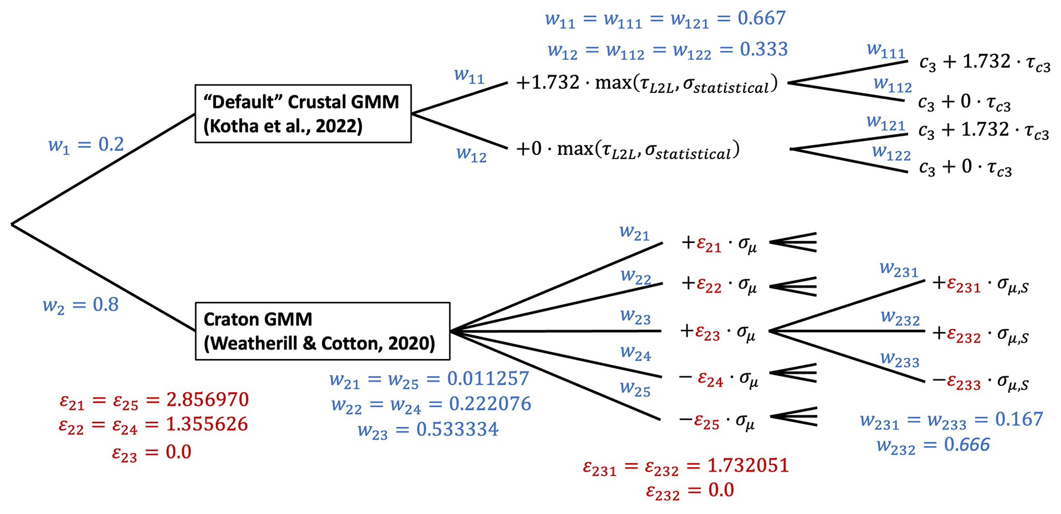
Figure 6Final ESHM20 GMM logic tree for application to the stable cratonic region of northeastern Europe.
Assessment of the final hazard results from the complete logic tree showed that the addition of the four branches from the default shallow-crustal-seismicity GMM reduces the seismic hazard at periods T < 0.3 s compared to using the CEUS logic tree, which is expected. However, both the CEUS logic tree and the proposed logic tree predict a significantly greater short-period hazard than that of the ESHM13, which is a result of the different amplification functions. For longer periods (T > 0.5) all three logic trees converge toward similar mean ground motions. The distribution of expected ground motions from the craton GMM logic tree is shown in Fig. 7 with respect to their attenuation with distance and their variation with spectral period.
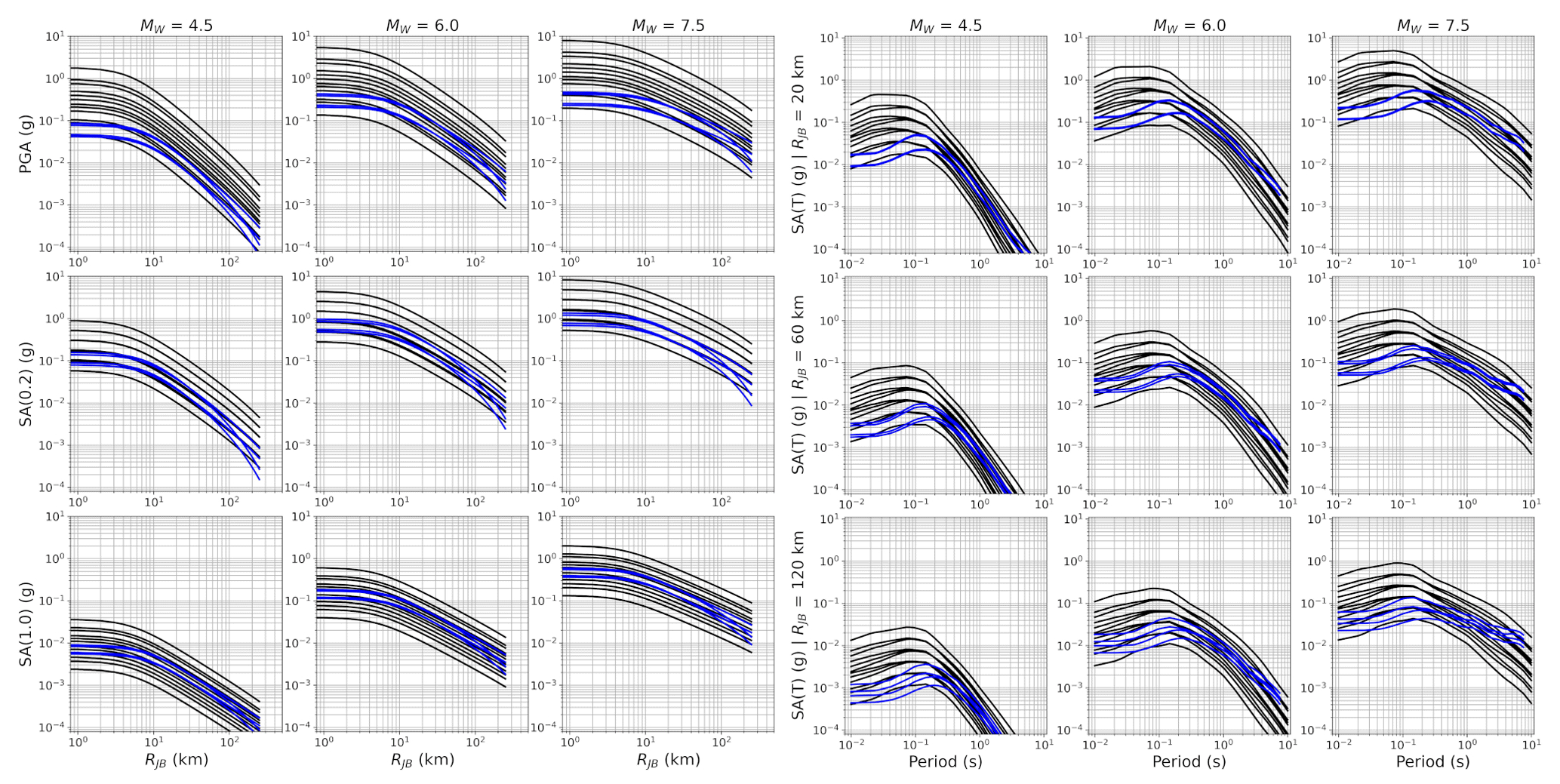
Figure 7As Fig. 3 but for the craton scaled-backbone GMM logic tree. Expected ground motions corresponding to the parametric craton model (Eq. 5) are shown in black, while the selected branches of the default shallow-seismicity model are in blue.
2.4 Site amplification and aleatory variability
Two important topics in the development and application of the GMM logic tree are the characterisation of the site amplification scaling in the models and the aleatory variability. The two are closely connected but have been addressed in parts across different publications. The form of the Kotha et al. (2020) GMM given in Eq. (1) does not contain an explicit site amplification term but contains instead the site-to-site residual (δS2SS). This is determined for more than 1829 stations across Europe, yet fewer than a third of these sites are associated with a measured VS30 in the original flatfile of Lanzano et al. (2019). Other site information, such as basin depth (and its various measures) or horizontal-to-vertical spectral ratio peak frequencies, was not compiled in ESM and is available from VS profiles for some sites in Switzerland, Italy and Türkiye. We therefore have many observations of site-to-site variability with respect to the median ground motion predicted by Eq. (1) but significantly fewer direct measures of predictor variables of site amplification. Additionally, the expansion of the number of recording stations integrated into the ESM database with respect to previous generations of ground motion records means that the data now contain records from a broader variety of geological and geotechnical conditions than before.
To include a site amplification scaling term into their model, Kotha et al. (2020) adopt two alternative functions: one is dependent on measured VS30, which is fit to the subset of 419 sites for which this parameter is available, and the other is dependent on scalar 30′′ slope at the site, which is available for all 1829 stations using Shuttle Radar Topography Mission digital elevation data. Both models adopt a quadratic site-scaling function:
where xpred is the predictor variable (i.e. VS30 (m s−1) or slope (m m−1)); xref a period-independent reference condition (VS30=800 m s−1 or slope = 0.1 m m−1); g0, g1 and g2 are period-dependent coefficients; and is the corrected site-to-site variability, which is shown to be smaller for the measured VS30 case. By limiting the data set to only those stations with measured VS30 and applying robust regression analysis, Kotha et al. (2020) return a lower compared to that of Kotha et al. (2016).
In the development of the ESRM20, Weatherill et al. (2023) addressed the issue of calibrating the site amplification for the context of the seismic risk calculations, with the requirement that ground motion must account for site response across all of Europe at a 30′′ scale. Starting with an updated topography/bathymetry model, a new pan-European map of VS30 inferred from slope was created using the approach of Wald and Allen (2007), which is complemented by a harmonised geology database for Europe compiled by BRGM. Using the regression outputs from Kotha et al. (2020) and selecting around 1100 stations for which δS2SS was constrained by three or more records, Weatherill et al. (2023) defined two different amplification models, one based on VS30 but whose coefficients and variability are dependent on whether the VS30 is measured or inferred from the slope proxy and the other using slope as the main predictor but introducing a geological-era classification as a random effect and thus making the implied amplification (but not its variability) dependent on both slope and geological era. In contrast to Kotha et al. (2020), Weatherill et al. (2023) adopt a two-segment piecewise linear function such that
where xpred is either measured or inferred VS30 or topographic slope, xref is now period-dependent, and xc describes a period-independent cut-off value above which fS is constant (fixed to VS30 1100 m s−1 when xpred=VS30 and slope 0.1 m m−1 when xpred= slope). In the VS30 case, the coefficients g1 and xref and the resulting site-to-site variance are dependent on whether the predictor is measured or inferred, with greater in the latter case. For the slope and geology case, g1 and xref are dependent on the geological era to which the site belongs, while is period-dependent but independent of geology and is found to be virtually identical to the inferred VS30 case.
Of the two formulations of the site amplification, it is that of Weatherill et al. (2023) that is adopted for ESHM20, although which of the predictors is used depends on the context of the application. For ESHM20 the requirement was to produce seismic hazard on a reference rock condition of VS30 800 m s−1 (Eurocode 8, Class A), which may be utilised as input into the Eurocode 8 design code itself. For design code application, amplification factors are specified explicitly in the code, and these are calibrated to allow for a margin of conservatism with respect to the amplification depending on whether the site class is defined from direct measurement or otherwise inferred. We specify that in this case VS30 must refer to a measured site condition in order to avoid double counting uncertainty that is already built into the amplification factors. For other applications in which the VS30 is either known directly or accurately inferred from detailed microzonation, the measured VS30 should be used. Otherwise, where VS30 is required but inferred from a larger-scale proxy such as topography and geology, the inferred VS30 form of the model should be used to ensure that uncertainty resulting from the use of the proxy is propagated into the hazard/risk calculations via the higher . For regional-scale risk in Europe in ESRM20, we adopted the form of the model based on slope and geology as we wanted to ensure that the amplification used in the risk model reflected the local geological condition, with higher amplification on deeper, younger Pleistocene and Holocene sediments and lower amplification on older consolidated rock. As was similar regardless of whether inferred VS30 is used as the predictor or slope and geology, it is ensured that uncertainty in amplification was being propagated via the GMM. Finally, the GMM and amplification model have been implemented in OpenQuake such that a partially non-ergodic total aleatory variability can adopted (i.e., and ϕS2S=0) where a site-specific site amplification model is available. Further explanation on all the above application contexts is given in Weatherill et al. (2021, 2023) and the underlying data sets accessed via the European Site Response Model Datasets Viewer (https://maps.eu-risk.eucentre.it/, last access: May 2024).
While site amplification and the role of site-to-site variability ϕS2S is a key component of aleatory uncertainty, further adjustments to the aleatory variability model of Kotha et al (2020) were made. Initially, the Kotha et al. (2020) GMM adopted a homoscedastic model of region-corrected between-event variability (τ0) and site-corrected within-event variability (ϕ0). Despite the transition of some variability from aleatory to epistemic uncertainty by moving τL2L and τc3 into the logic tree and the adoption of robust mixed-effects regression to downweigh outlier observations in fitting the fixed effects, the remaining variability was still large compared to previous models. However, this variability is controlled by the small-magnitude events, which prompted further exploration into the question of heteroskedasticity in the between-event and within-event variability. From this, Weatherill et al. (2020) proposed adopting a magnitude-dependent heteroskedastic aleatory uncertainty model for τ0 and ϕ0. The former was adopted directly from an analysis of global ground motion records by Al Atik (2015), while the latter also adopted form Al Atik (2015) but recalibrated to fit observed ϕ0 at smaller magnitudes. Subsequently, Kotha et al. (2022) subjected their model to a more formal statistical analysis for heteroskedasticity using the Breusch and Pagan (1979) test, which also confirmed the presence of apparent heteroskedasticity in the between- and within-event residuals. Their proposed model is similar in structure and extent to that already adopted by Weatherill et al. (2020); however, both could be applicable. The between-event residuals were also scrutinised for distance-dependent heteroskedasticity and the site residuals for VS30-dependent heteroskedasticity, but no compelling trends were apparent in these cases. The final aleatory uncertainty model therefore retains only the heteroskedastic τ0(Mw,T) and ϕ0(Mw,T) presented in Weatherill et al. (2020). A case could be made for further exploration of the epistemic uncertainty into the aleatory σT term; however, given the already considerable size of the GMM logic tree, this was not pursued in ESHM20.
2.5 Subsequent development and considerations for implementation
While the previous sections have outlined the overall framework behind the regionalised scaled-backbone GMM logic trees for both non-craton and cratonic seismicity, there were several feedbacks and lessons learned from application of the model to seismic hazard in Europe. These feedbacks were incorporated into the final ESHM20 and ESRM20 calculations, so we summarise the most significant ones here.
2.5.1 Adaptations to the backbone GMM (Kotha et al., 2022)
The backbone GMM as it is described in Kotha et al. (2020) applies a hinge magnitude, Mh, to capture the break in magnitude scaling from quadratic (for Mw < Mh) to linear (for Mw ≥ Mh) at magnitudes greater than Mh= 6.2. This number was originally based on non-parametric analysis of the magnitude scaling implied by the ESM data set; however, data from larger earthquakes were limited to a relatively small number of large events from Italy and Türkiye. At the same time, when compared to its predecessor European database of strong motions, the ESM contains more than 10 000 new records from earthquakes with magnitudes M ≤ 4.5, for which very few direct moment magnitudes (Mw) are present. Although Kotha et al. (2020) used a harmonised moment magnitude from the updated European-Mediterranean Earthquake Catalogue (EMEC) (Grünthal and Wahlström, 2012; updated in Danciu et al., 2021), these magnitudes are equivalent proxy magnitudes converted from their originally recorded scales. When fitting the GMM, these factors, and potentially others, resulted in a positive b2 coefficient in their model for short periods, which in turn produced a flattening of the magnitude scaling at low magnitudes, a kink in the magnitude scaling at magnitudes Mw≈Mh and a more strongly negative trend in the ground motions for Mw>Mh (the result of a negative b3 term in Eq. 2). These effects contributed to a more significant weakening of ground motions for larger magnitudes at short distances (apparent oversaturation), along with a higher σstatistical, compared to other GMMs.
Following the publication of the Kotha et al. (2020) GMM and based on further exploration and comparison of the models using the NEar-Source Strong-motion data set NESS (Pacor et al., 2018; Sgobba et al., 2021), it was found that the negative scaling of b3 yielded a moderate bias in between-event residuals for large-magnitude earthquakes. Revision of the period-independent Mh from Mw 6.2 to Mw 5.7 was shown to reduce this bias and, in doing so, also reduce σstatistical for larger-magnitude events. The analysis and motivations for revising Mh, along with a more detailed comparison of the models against the NESS data set, can be seen in Kotha et al. (2022). Given the relatively small proportion of the data set affected by the change Mh, the influence on the random-effect residual terms that form the basis for the regionalised scaled-backbone logic tree (described previously, and in Weatherill et al., 2020) was found to be negligible. The final ESHM20 model adopts the modifications to the median ground motion model from Kotha et al. (2022) rather than the original model of Kotha et al. (2020).
2.5.2 Logic tree implementation and computation
The GMM logic trees for shallow seismicity that have been presented in this section were among the first products of ESHM20 to be completed. While the description of the logic trees provided in Weatherill et al. (2020) and Weatherill and Cotton (2020) remains largely accurate in terms of construction, some minor modifications were made after the first iteration of the complete seismic hazard model. Firstly, while Weatherill et al. (2020) had proposed using three branches each of the tectonic-locality uncertainty and the attenuation region uncertainty, it was found that the tectonic-locality uncertainty was the dominant epistemic uncertainty for most regions, with residual-attenuation region uncertainty only manifesting in the distributions in cases where hazard is dominated by active sources at more than 100 km away from a site. This tended to result in clustering of the hazard values into three areas around each of the three tectonic-locality branches, which would then produce 84th and 95th percentile hazards that were virtually identical. Given the importance of the tectonic-locality uncertainty, we choose to discretise it into five branches using the approximation of Miller and Rice (1983) rather than the originally proposed three branches. For the attenuation region, the three-branch approximation was retained as this had a relatively minor influence on the seismic hazard. This same strategy is applied to the craton logic tree case, where σμ is discretised into five branches and σμ,S is retained as three branches. Discrete representations using higher numbers of branches were considered, which, though desirable from the point of view of accuracy in representing the epistemic uncertainty, incurred too great a computational cost.
The second adaptation of the logic tree is an implementation detail that redefines how the residual-attenuation adjustment is treated compared to its original intention. Weatherill et al. (2020) explain the problem of permuting logic tree branches when we have regionalisation in the model, with the challenges being that if we define the region as an attribute of the location in which the earthquake is found and the logic tree considers each branch of each region independently, then we would need total end branches to describe exhaustively the combination of permutations of logic tree branches. This has been the standard approach for many regional hazard models including ESHM13. Originally, Kotha et al. (2020) define δc3 for 42 zones, which had we described a separate logic tree for each region would have resulted in 43 branch sets (including the default). Thus, with the original proposal of 9 branches per branch set we would reach 943 end branches. Applying the hierarchical clustering reduced this to a more manageable 96=531 441 branches, although we would need to apply the same to the craton, subduction interface, subduction in-slab and non-subduction deep regions, which would yield 910=3486 784 401 branches. In reality, no single location is affected by earthquakes originating in seismogenic sources from all regions, and the number varies from simply 9 branches (much of northwestern Europe) to 97=4 782 969 branches (Albania and western Greece). Although in the calculations the logic tree would not evaluate all branches but sample instead several tens of thousands, simply defining the set of branches from which to sample was causing computational challenges, that were not justified given that the attenuation uncertainty was not dominant.
To resolve the problem of excessive branches, we changed strategy and implemented the regionalisation as a property of the target site rather than of the source. Here, all sources are assigned to a single tectonic region type (shallow default) in the files, and the residual-attenuation adjustments will be applied depending on the region (from the Basili et al., 2021, regionalisation) in which the site is found. This redefinition is relevant for two reasons – the first is that this is more consistent with how δc3 was defined in the regression (recall it was a property of the region in which the station was located) and the second is that this allows us to apply the adjustments over all regions simultaneously. This last point means that we reduce the non-cratonic shallow-crustal-seismicity GMM logic tree from 531 331 branches to just 9 branches, which allowed us to then increase the number of tectonic-locality distribution branches from three to five in order to better capture differences in the outer quantiles. We still need to apply the regionalisation to the other regions considered (i.e., craton, subduction interface, subduction in-slab and non-subduction deep seismicity) but the total GMM logic tree now contains end branches – many orders of magnitude fewer than before. This is inevitably still large, but now it becomes feasible to calculate and is significantly further reduced in areas of Europe where subduction or deep earthquakes are not relevant for hazard. There is, however, a theoretical cost to this decision, which is that the same residual-attenuation adjustments (e.g., , ) are applied over all sites at the same time. This introduces an artificial correlation, and there could exist the possibility for sudden changes in hazards across the boundaries of some regions. However, given that the residual attenuation is not the dominant uncertainty, for areas where many residual-attenuation regions may be influencing seismic hazard, the seismicity is usually high and thus the controlling earthquakes are nearer to the source. After inspection of the results, we were satisfied that the benefits of the change outweighed the potential costs.
Although the general framework for the GMM logic tree has been laid out in the previous section and in the preceding publications, in certain regions there have been additional adaptations to this that were implemented in response to feedback from local scientists and engineers. In each of these cases the adaptations have been based on analysis of additional data that were not contained within the ESM database used by Kotha et al. (2020, 2022) to define the backbone GMM.
3.1 Slow-attenuation regions in western Europe
The residual-attenuation term δc3 was determined for 42 out of 110 zones, mostly located in Italy, Switzerland, Greece, Türkiye, and the Balkans. Two zones in particular stand out from the others as featuring particularly slow anelastic attenuation, both of which are well constrained by the data in the zones: (1) the Pyrenees and northern Spain and (2) eastern Romania and southern Ukraine. The exact cause of this slow attenuation is not clear from the ESM data set, and while consultation of the additional geophysical data sets used to define the cratonic region of Europe raised some possibilities, a consistent explanation was not forthcoming. For the eastern Romania and southern Ukraine case, this slow-attenuation region may represent the transition point between the faster attenuation observed to the south and west and the very slow attenuation in the cratonic region across the TESZ to the north and east. This same explanation does not apply to the Pyrenees, however, and the transition from slightly slower than average attenuation in the Alps to particularly slow attenuation in the Pyrenees occurs over a relatively short distance. The spatial pattern of attenuation in France therefore may have particularly interesting implications for seismic hazard across much of western Europe.
Running concurrent to the development of the ESHM20 was the Research and Development Program on Seismic Ground Motion Assessment (SIGMA 2) project, which undertook further investigation of seismic ground motion in France using the Réseau Sismologique et Géodésique Français (Résif) ground motion data set (Traversa et al., 2020). The Résif database contains more than 6500 records from 468 earthquakes recorded at 379 stations within metropolitan France. The magnitude distribution of these earthquakes is between 2.0 and is generally skewed toward a lower range of magnitudes than that of the ESM data set. Kotha and Traversa (2024) extends the analysis presented in Kotha et al. (2020) to include the Résif data, providing both δL2Ll and δc3 for regions in France that were not well constrained by the ESM data (Fig. 8). The new analysis using the Résif data set broadly confirmed the trends implied from the ESM data for δc3, with attenuation significantly slower in the Pyrenees than in southeastern France.
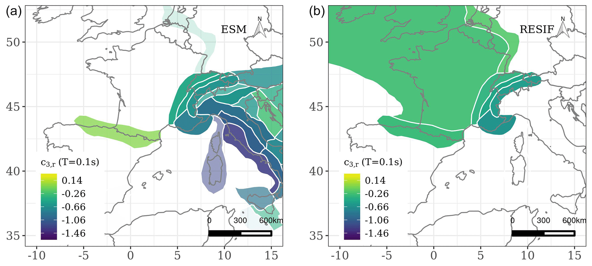
Figure 8Distributions of δc3,R for T≈0.1 s calibrated according to the ESM database (a) and the Résif database (b). Figure adapted from Kotha (2020).
Although the Résif database contains more data in central and northern France, including new stations closer to the Rhine Graben, one limiting factor is that in the assumed regionalisation of apparent anelastic attenuation via δc3,r, all of central and northern France, Belgium and the United Kingdom are grouped into a single zone. The analysis of Kotha and Traversa (2024) therefore only confirms that attenuation in much of this region is slower and potentially comparable to that found in the Pyrenees zone in the original ESM data, but it does not resolve further geographical variation. Further insights into the spatial variation in France were possible due to the tomographic study of Mayor et al. (2018), which mapped variation in absorption Qc across France. These data highlighted areas of slow attenuation corresponding to the Armorican Massif (northwestern France), the Massif Central (central and southern France) and the Ardennes Massif, all areas of predominantly Paleozoic basement contemporaneous with that of the Pyrenees.
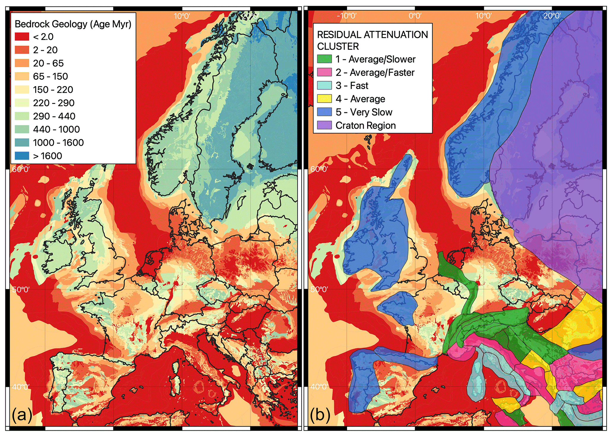
Figure 9Bedrock geology across Europe from the 1:5 000 000 International Geological Map of Europe (Asch, 2005) coloured according to age (a) and updated regionalisation depicting the final spatial extent of the slow-attenuation cluster (b).
Assembling the multiple lines of evidence from the analyses of Kotha (2020) and Mayor et al. (2018) and consulting the 1:5 000 000 International Geological Map of Europe (Asch, 2005) (Fig. 9, left), we delineate an additional set of regions across western Europe that we believe may be represented by the slow-attenuation region (cluster 5) that was previously applied to the Pyrenees. This regionalisation is shown in Fig. 9 (right). Beginning in southern Portugal (which will be discussed in due course), the slow-attenuation region follows the line of predominantly Paleozoic (pre-Variscan) geological units north through Portugal and northern Iberia into the Pyrenees. The Aquitaine Basin interrupts this region, but it is then resumed with the Armorican Massif and continues through the northern and western British Isles. Finally, we also add into this regionalisation Scandinavia west of the Caledonian orogeny that indicates the western limit of the cratonic Baltic Shield. Although there is also evidence that could suggest including the Massif Central into this delineation, we take the decision to keep it in the default shallow-seismicity region and not necessarily within the slow-attenuation zones. This is to allow for a smoother transition in attenuation across southern France rather than abutting the very slow attenuation zone against the faster zones in southeastern France and the Alps. Further exploration of the spatial variation in attenuation using a higher-resolution (or more refined) set of zones may help in refining the regionalisation of attenuation across France and Iberia in the future (Kotha and Traversa, 2024).
3.2 Offshore Atlantic sources (Portugal)
A particularly critical area for seismic hazard in Europe is southern Portugal, where large earthquakes have occurred close to the Strait of Gibraltar several times throughout recorded history, including the destructive 1755 Lisbon earthquake (Mw 8.5±0.3, Rovida et al., 2022) and damaging 1969 Portugal earthquake (Mw 7.8). Observations of ground shaking from these offshore events are usually measured at stations more than 100 km from the earthquake source, but previous analysis of these records and those of other onshore Portuguese earthquakes has suggested that the region may be better modelled using GMMs from stable continental (cratonic) regions than those from active regions (Vilanova et al. 2012). This is in part due to the slow attenuation of such events along their travel path through the predominantly stable continental crust. However, applying such GMMs to onshore earthquake sources in southern Portugal is more challenging, because while analysis by Vilanova et al. (2012) of spatial patterns of intensity slightly favoured stable cratonic GMMs over inter-plate GMMs for use, there is high uncertainty. When executed in a scenario of seismic risk calculation for a Mw 5.7 earthquake close to Lisbon on the Tagus Valley fault, however, use of stable continental GMMs resulted in a factor-of-2 increase in losses with respect to those scenario calculations using active shallow-crustal-seismicity GMMs (Silva, 2016). This suggests that the impact of the stable craton GMMs can be particularly large in this region.
Unfortunately, too few records from Portugal were included in the ESM to allow constraint of δL2ll and δc3,r in this region in the development of Kotha et al. (2020), but given the importance of this region for seismic hazard and risk in southern Portugal, further analysis was warranted. We returned to the earlier RESORCE database of strong ground motions (Akkar et al., 2014b), where more Portuguese strong-motion records were available, and identified 42 records from which we attempt to make comparisons against (1) the default shallow-crustal-seismicity logic tree, (2) the shallow-crustal-seismicity logic tree for the very slow attenuation cluster, and (3) the GMM logic tree for the parametric craton model (Weatherill and Cotton, 2020). Figure 10 shows the magnitude–distance–VS30 composition of the data set (where VS30 is largely assigned from topographic proxy), indicating that all but one record is recorded at a distance greater than 100 km.
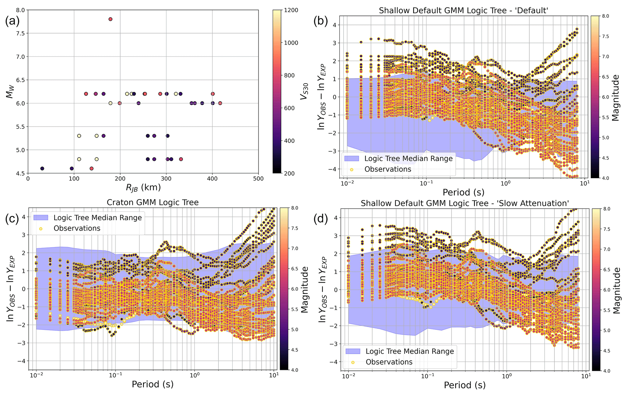
Figure 10Magnitude and distance distribution of Portuguese records from RESORCE used for the analysis (a) and comparison of the distribution with the period of residuals of observed ground motions with respect to the backbone GMM for the default shallow GMM logic tree (b), the craton GMM logic tree (c) and the slow-attenuation cluster GMM logic tree (d). The shaded regions describe the range of expected ground motions from the logic tree across all the considered scenarios, centred such that 0 describes the unadjusted backbone GMM for each logic tree. Points corresponding to ln (YOBS)−ln (Yexp) are colour scales according to the earthquake magnitude.
To make the comparisons we compare the distributions of observed ground motion against the ranges of median ground motions implied by the different logic trees, also shown in Fig. 10. A clear period-dependent trend is available in the comparisons with observations toward the upper end of the range of the median ground motions expected from the default shallow-crustal-seismicity logic tree at short periods, but then trending strongly toward lower-than-expected values at longer periods. As discussed in Vilanova et al. (2012), for many of the accelerometer records the signal does not exceed the required signal-to-noise ratio for periods longer than ≈ 0.9 s, so long-period trends should be interpreted with caution here. The comparisons do show, however, that when switching to the very slow attenuation form of the model the centres of the distributions of observations at short periods do move closer to the centre of the distribution predicted by the model, but the trend remains positive, indicating some systematic underestimation. Comparing against the craton GMM logic tree we then see a tendency toward slightly negative residuals across the whole spectrum, indicating a systematic overestimation of higher-frequency motion with this logic tree. Interestingly, the residuals seem to suggest higher-than-predicted ground motions at smaller magnitudes (Mw≤5) than at larger magnitudes, which could imply differences in stress drop scaling, biases from the conversion from local or body wave magnitude to Mw, or simply biases in the record selection due to weaker records from these earthquakes producing insufficiently high signal-to-noise ratios to retrieve spectra.
This limited, yet somewhat insightful, analysis reflects the trends seen by Vilanova et al. (2012), which shows that ground motions from these offshore earthquakes are better described by models with slower attenuation than that normally predicted by GMMs for active shallow regions. We reiterate, however, that these comparisons show the distributions of the median ground motions, and very likely most, if not all, of the records would fall comfortably within the range of motions when including the standard deviations. A potential case for switching entirely to the cratonic GMM logic tree in this region could be made, but it is not fully clear either and may risk systematic overestimation of ground motions for larger magnitudes at short distances, which would be the scenarios likely to control hazard for return periods of engineering interest. We therefore opt for a compromise solution by adopting the very slow attenuation regionalisation of the non-cratonic seismicity logic tree rather than the parametric craton model. For local- and national-scale PSHA in Portugal it may be recommendable to consider both sets of logic tree branches in a larger GMM logic tree, which might be a fairer reflection of the degree of epistemic uncertainty. Computational challenges in implementation prevent us from exploring this possibility entirely in the ESHM20, however, so we place onshore Portugal into the same very slow attenuation cluster that is applied for much of western Iberia, France and the British Isles described previously.
3.3 Iceland
The third special case region that was adapted after the preliminary calculations of seismic hazards is that of Iceland. Similar to Portugal, this was a region for which existing strong-motion records had not been included or made available to ESM and were therefore not regionalised in the development of Kotha et al. (2020, 2022). With its rapid tectonic deformation and extensive volcanism, Iceland itself is arguably an outlier for ground motions compared to the other active seismicity regions in Europe. A strong-motion network has been in operation since 1984 (Sigbjörnsson et al., 2009), and observations from moderate-to-large-magnitude events have suggested that the region is associated with shallower seismicity and faster attenuation than other active regions (Ornthammarath et al., 2011; Kowsari et al., 2019, 2020). This was acknowledged, to a certain extent, in the original formulation of the regionalised backbone GMM logic tree by Weatherill et al. (2020), who identified a predominance of ground motion records with partially volcanic travel paths (or paths through regions of higher heat flow) as a common factor behind the low δc3,r values in the regions assigned to the fast-attenuation cluster. It was originally proposed to apply the fast-attenuation δc3,r adjustments to onshore source zones in Iceland too, even though Icelandic data were not present in ESM. Feedback from local experts in the region, along with recently published GMMs for Iceland (Kowsari et al., 2019, 2020, 2023), prompted us to revisit the GMM logic tree here.
While the Icelandic strong-motion data were not available to ESM, records had been made available in the earlier RESORCE database (Akkar et al., 2014b). The distribution of records with respect to magnitude, distance and geographic location is shown in Fig. 11. Choosing to limit the data to well-recorded earthquakes with constrained Mw, the data used in the current analysis contain 120 records from 18 events with magnitudes in the range 4.5 6.5, and distances in the range . As seen in the geographical distribution, the data come predominantly from two regions: the South Iceland Seismic Zone (SISZ) and the Tjörnes Fracture Zone (TFZ) in northern Iceland. Only 11 of the 120 recordings used come from the TFZ, so we limit our analysis only to those from the SISZ.
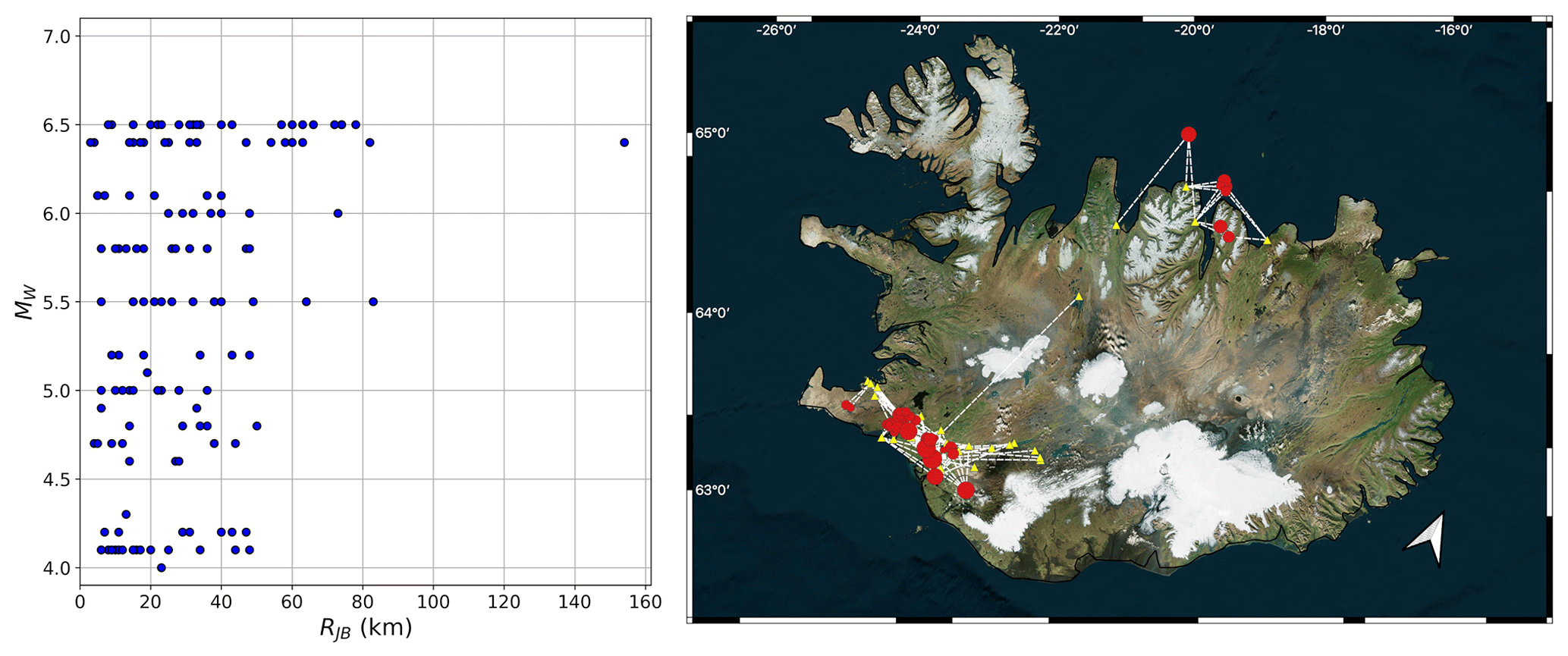
Figure 11Distribution of Icelandic ground motion records found in the RESORCE database and used in the current comparison. Magnitude–distance distribution (left) and geographic distribution (right). Figure adapted from Danciu et al. (2021).
As differences in the record processing and metadata compilation were present, we did not wish to attempt to retrieve δc3 and δL2Ll by rerunning the Kotha et al. (2020) regression to avoid these regional differences in the data contaminating the fixed effects. Instead, we undertook an a posteriori analysis to retrieve the normalised between-event and within-event residuals with respect to the backbone GMM and its proposed adjustments, using the estimators of δBe(T) and δWes(T) described in Stafford et al. (2008). This also allowed us to compute the residual with respect to other GMMs proposed for application to Iceland by Kowsari et al. (2019). The normalised within-event residuals were inspected for trends with distance with respect to different branches of the GMM logic tree representing different adjustments to the model. Although we have few records for distances greater than 80 km, where we would expect the δc3,r to play a greater role, we find that the distance trend indicated attenuation that was faster than the average condition from Kotha et al. (2020) at short periods but that application of the cluster 3 (fast attenuation) calibration was adequate to correct for this trend. The observed variability of the within-event residuals was lower (≈ 80 % of the full within-event variability implied by the ESHM20 GMMs), but this is likely a reflection of the limited data set and predominance of travel paths across the same single region.
For δBe(T) a stronger trend could be seen in the residuals with the spectral period, with short-period motion giving predominantly negative δBe(T) and gradually transitioning toward positive δBe(T) for longer periods with T≥1 s. Comparisons against the different adjustments to the Kotha et al. (2020) model revealed that for short periods the low stress adjustment provided the least biased prediction of normalised residuals ( for , passing to the average model close to T= 1 s ( for ) and the high stress model for T≥2 s ( for . The distribution of δBe(T) is shown in Fig. 12. Given that the data set contained records from only 18 events, dependence of these trends with respect to magnitude could not be confirmed and was not immediately apparent. This analysis suggests that there is evidence for systematic differences in the ground motions in the SISZ with respect to the Kotha et al. (2020) model (and its adjustments) but that this is strongly period dependent and not well represented by the current δL2Ll branch logic tree. There could be several causes behind this, including systematic site effects or depth dependence being captured by δBe, and we cannot neglect the possibility of bias in the magnitude estimation propagating into the between-event residual. Further investigation of these questions should be the focus of future research; however, with the information we have at present, we opted to create a local δL2Ll to be applied in Iceland.
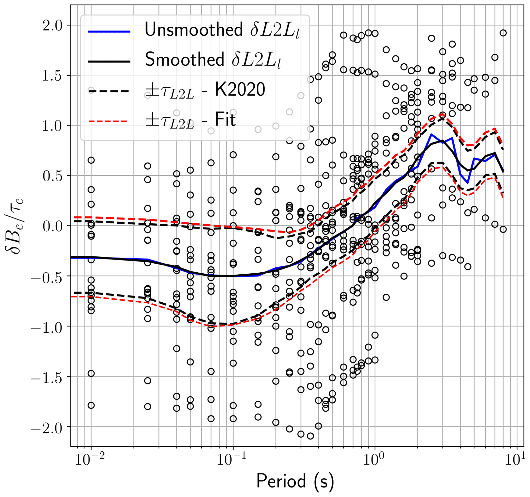
Figure 12Distribution of between-event residuals with period for the Iceland ground motion data, with fit models of δL2Ll(T) and its variability τL2L.
To calibrate the regional adjustment, we take the observed trends in δBe with residual and use Bayesian fitting of the Gaussian model via a Markov chain Monte Carlo approach (Salvatier et al., 2016) as had been applied to retrieve the cluster-specific δc3,cl distributions for the residual attenuation. A prior distribution of N(0,τL2L(T)) is used for the mean δL2Ll and for the standard deviation. The posterior mean δL2Ll and its standard deviation are shown for each period in Fig. 12, and the values are smoothed to reduce excessive period-to-period variability at longer periods. From the data available the mean δL2Ll is updated clearly to reflect the period-dependent trend, while the τL2L does not update the prior significantly, potentially because too few events represented in the data set exist.
To construct the region-specific logic tree for Iceland, we map the posterior distribution of δL2Ll into the corresponding branch set (), while for the residual-attenuation branches we adopt the cluster-region-specific δc3,cl for cluster 3 (fast attenuation). Although the adjustment factors are calibrated based exclusively on data from the SISZ, they are applied to all onshore sources in Iceland, as well as to the offshore source zones representing the mid-Atlantic ridge to the south and to the north of the island. All other offshore sources were assigned the default shallow backbone GMM logic tree. This adjustment has the effect of reducing short-period hazard with respect to using the original GMM logic tree increasing hazard at long periods. For the implementation of the model in ESHM20 we note that this adjustment would technically make Iceland a new tectonic region, requiring its own GMM logic tree that would multiply the total number of logic tree branches by a factor of 15. We take advantage of geography, however, to treat Iceland separately from the calculations for the rest of Europe for the purposes of the ESHM20 calculations, which we do by running it as a stand-alone model in a separate calculation. This reduces the calculation to only the 225 GMM logic tree branches (15 from the Iceland-adjusted GMM logic tree applied to onshore and mid-Atlantic ridge sources, 15 from the original shallow-crustal-seismicity GMM applied to the stable offshore sources), allowing for faster and more convenient computation.
The three cases discussed in this section (France, Portugal and Iceland) illustrate how it was possible to take decisions and make modifications to the logic tree on the basis of other ground motion data not contained within the original ESM data set used to fit the shallow backbone GMM and its regionalisation. This shows that the approach can be flexible and that the backbone GMM can accommodate further regional adjustments when there is a sufficient basis to do so. Further discussion around the issue of adaptability of the regionalised GMM logic tree approach can be found in the concluding Sect. 5.
While much of the efforts toward developing the regionalised backbone GMM concept have focused on shallow seismicity, for several regions of Europe the earthquakes that control the hazard come from deeper seismicity or from subduction zones. This includes the Hellenic, Cypriot and Calabrian arcs as well as the Gibraltar Arc (added now in ESHM20 as a deep subduction source) and the Vrancea deep seismic zone. As the ESM flatfile contains thousands of records from Greece, Türkiye and southern Italy, inevitably a proportion of the waveforms are from subduction zone or non-subduction deep seismicity sources. It is well established that the source and path characteristics of strong ground motions originating from subduction earthquakes differ significantly from those of earthquakes in the shallow crust (e.g., Youngs et al., 1997; Atkinson and Boore, 2003, Hassani and Atkinson, 2021), and previous seismic hazard models in Europe have assigned subduction GMMs to such sources. The ESHM13, for instance, adopted a multi-model GMM logic tree comprising the subduction GMMs of Youngs et al. (1997), Atkinson and Boore (2003), Zhao et al. (2006) and Lin and Lee (2008), which were selected and weighted based on both expert judgement and log-likelihood analysis using a limited set of 65 recordings from only in-slab earthquakes (Delavaud et al., 2012). Similarly, Pavel et al. (2016) adopted global subduction in-slab GMMs for application to the Vrancea seismic zone (Youngs et al., 1997; Atkinson and Boore, 2003; Abrahamson et al., 2016) alongside a local GMM calibrated specifically to records from large Vrancea earthquakes (Vacareanu et al., 2015). Because of the differences in source, path and site characteristics, we cannot treat subduction and deep source seismicity as a special case adaptation of the shallow GMM logic tree, and instead it requires its own development approach that leverages on the existing data and subduction GMMs from around the globe.
In this section we present the construction of a backbone GMM logic tree for application to the subduction and deep seismicity regions of Europe. As will be shown in due course, the objectives of the backbone GMM logic tree in capturing epistemic uncertainty in GMM stress parameter and attenuation are shared with those of the regionalised backbone GMM adopted for non-cratonic shallow seismicity. However, while ESM contained a large volume of data from shallow seismicity to fit and calibrate the backbone GMM, the number of records from deeper earthquakes is far smaller and covers a more limited range of magnitudes compared to those needed for the hazard model. As such, we cannot develop a new GMM for subduction and deep seismicity but define the regionalised backbone by first identifying a suitable candidate GMM based on a combination of judgement and fit to observed data, before then using the observations to calibrate the attenuation characteristics of the GMM to better match the local attenuation properties inferred from that same data set. Finally, we consider region-to-region variability in source stress parameter and anelastic attenuation components of subduction GMMs globally as a basis for defining and weighting the adjustment factors to the model.
4.1 Classifying records from subduction and deep seismicity earthquakes
Our first challenge in the development of the subduction backbone GMM for application in Europe is to identify those records from subduction and/or non-subduction deep seismicity. In its original form described by Lanzano et al. (2019), the ESM did not have a tectonic region classifier in the records, nor was a focal mechanism available for small-to-moderate-magnitude earthquakes. Several different approaches toward subduction event classification have been attempted in the development of existing ground motion models (e.g., Atkinson and Boore, 2003; Zhao et al., 2006; Abrahamson et al., 2016, 2018), many of which rely on a combination of depth, focal mechanism and proximity to the modelled subducting slab geometry using Slab 1.0 or 2.0 (Hayes et al., 2018). In the Vrancea deep seismicity region, a relatively clear separation can be seen between the distribution of hypocentral depths associated with the deep seismogenic source (60 ≤hD (km) ≤ 180) and those associated with crustal seismicity (hD≤ 30 km). The relatively small number of earthquakes from the Vrancea region in the ESM, combined with their clear localisation to the Vrancea deep source, made it possible to identify and extract records from deep seismicity in Vrancea manually. For the subduction regions in the eastern Mediterranean, however, a different approach was needed.
In comparison to many subduction zones around the globe, the Hellenic, Calabrian and Cypriot arcs display a modest rate of seismicity, with very few large interface and/or in-slab events since the establishment of strong-motion recording networks in the region. As such, most of the observed ground motion data come from small to moderate seismicity in the eastern Mediterranean region, for which 3D rupture models are unavailable, focal mechanisms are limited, and potentially significant uncertainties are present in location and depth (albeit the error estimates are not always reported). This combination of factors prompted us to develop a subduction region classification approach that allows for an often-unquantified uncertainty in many attributes of the seismicity and of the subduction geometry itself. We therefore developed a fuzzy rule-based classifier that expands on previous fuzzy regionalisation concepts presented by Chen et al. (2018).
The core of the classifier is the idealised conceptualisation of the subduction system, which is illustrated in Fig. 13. Within this system we identify six classes of seismicity: shallow crust, subduction interface, subduction in-slab, upper-mantle wedge and outer rise, and non-subduction deep seismicity. While the distinction between interface, in-slab and shallow crust should be unambiguous in this system, our uncertainties on slab geometry, earthquake location within the subduction system and their respective focal mechanisms mean that our classification cannot be crisp, i.e. unambiguous and unique. The boundaries from slab to mantle wedge to crust or from slab to outer rise also contain a degree of ambiguity. With this ambiguity present and uncertainties on locations that are inconsistently reported and therefore not often numerically quantified, we use fuzzy inference because it allows us to translate expert-driven judgements or degrees of belief into a quantitative and reproducible system for classification.
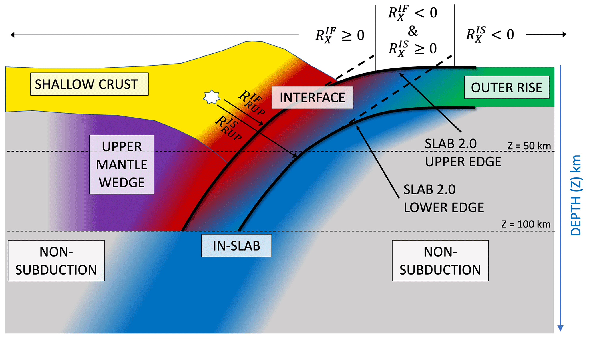
Figure 13Conceptualisation of the subduction zone system for the fuzzy classifier, with regions and distance metrics , , and (as described in body text) illustrated and the earthquake hypocentre shown with a star.
The fuzzy rule-based classifier begins by encoding quantitative values of multiple input data into fuzzy classifications via a set of antecedent rules that define membership of the data to descriptive categories, e.g., whether an earthquake is DEEP or SHALLOW, NEAR to an interface or FAR from it, among others. The antecedent rules are combined with a set of consequent rules that define quantitative function to map the outcome (i.e., the tectonic class) to a degree of membership (i.e., LOW, MEDIUM, HIGH). The antecedent and consequent rules are input together into a control system where multiple antecedent rules can be joined using logical statements/rules and mapped to corresponding consequents, e.g. “If DEPTH is DEEP and REVERSE [Faulting] is LOW then IN-SLAB is HIGH”. When defined by the set of rules and fed with the necessary input parameters, the control system returns for each observation a degree of membership to each tectonic class between 0 (unambiguously not belonging to this tectonic class) and 1 (unambiguously belonging to this tectonic class). While the degrees of membership may themselves be fuzzy, we still require a final tectonic classification for each earthquake in the ESM; i.e. the final output must be defuzzified in order to assign a single outcome or class. This final tectonic classification is made according to the criteria (i) that the tectonic class to which the event is assigned should be that with the highest degree of membership among all considered classes, (ii) that this same degree of membership for the event in this class is ≥ 0.6 and (iii) that the degree of membership to the next highest membership class is < 0.4.
From the ESM flatfile, the earthquake parameters available are the magnitude (as reported by the original source agency), location and depth estimate for nearly every event. Focal mechanisms were not included for the events initially (only a qualitative style of faulting where available); however, corresponding focal mechanisms for events were retrieved from national and regional databases. This provided focal mechanisms for nearly all earthquakes with magnitude Mw > 4.8; however, for many smaller earthquakes no moment tensor was available. For the slab geometry, we had available slab upper-surface definitions from Slab 2.0 (Hayes et al., 2018) for the Hellenic/Cypriot and Calabrian arcs. The ESM lacked any records from deep seismicity in the Gibraltar Arc, so this region is not considered any further. A lower slab surface is defined by projecting the upper surface downward in the slab normal direction assuming a given slab thickness. We adopted a fixed thickness of 50 km, which we inferred from the distribution of seismicity.
Two control systems were constructed: one for the case in which the earthquake has a focal mechanism (or rake from style of faulting) and one in which it does not. For both cases the input parameters required are the hypocentral depth, the average of the distance between earthquake source and the upper slab surface (), the distance between the earthquake source and the lower slab surface () , the difference between these two distances , and finally the along-surface distance between the epicentre location and up-dip projection (with respect to dip at a given depth contour) of the upper interface and lower interface respectively ( and ). Where focal mechanism or assigned style of faulting is present, the rake is input into the fuzzy classifier. These parameters are illustrated with respect to the subduction model in Fig. 13 and the corresponding antecedent rules in Fig. 14. Events located more than 500 km from the Slab 2.0 subduction surface were automatically classified as non-subduction and not run through the classifier. For events in the Ionian Sea, western Greece and Puglia (also known as Apulia), the classifier was run twice, once with respect to the Hellenic subduction and once with respect to the Calabrian subduction, and the tectonic classification is made on the basis of the highest membership from either of the two subductions. We could not identify any highly ambiguous cases in which the tectonic classification changed significantly depending on the subduction zone to which the classifier is applied.
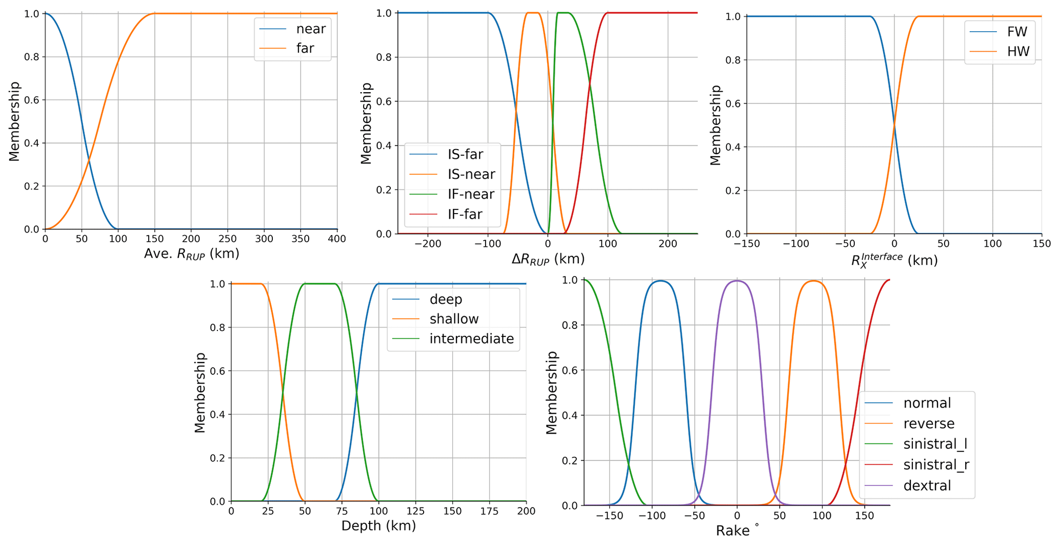
The fuzzy classification system was in fact originally applied to the ESM database prior to the development of the Kotha et al. (2020) backbone GMM for shallow-crustal-seismicity earthquakes to remove the subduction and deep seismicity from that set of records. Application of the classifier to 2179 earthquakes in the ESM database yielded 209 interface earthquakes, 133 in-slab, 12 outer rise events and 5 upper-mantle earthquakes. The remainder are classified as non-subduction, which were then restricted to just the set of shallow earthquakes by Kotha et al. (2020) using the criteria mentioned previously. Once classified, other selection filters were applied to the data to exclude events of small magnitude (Mw < 4.0), events for which no homogenous magnitude could be defined from the EMEC catalogue, and other events for which only single records exist or all records are found at distances greater than 300 km. The final set of non-shallow ground motions comprises 684 records from 164 subduction interface events, 704 records from subduction in-slab events and 938 records from 64 Vrancea deep source events. The magnitude and distance distributions of these three subsets of records are shown in Fig. 15.
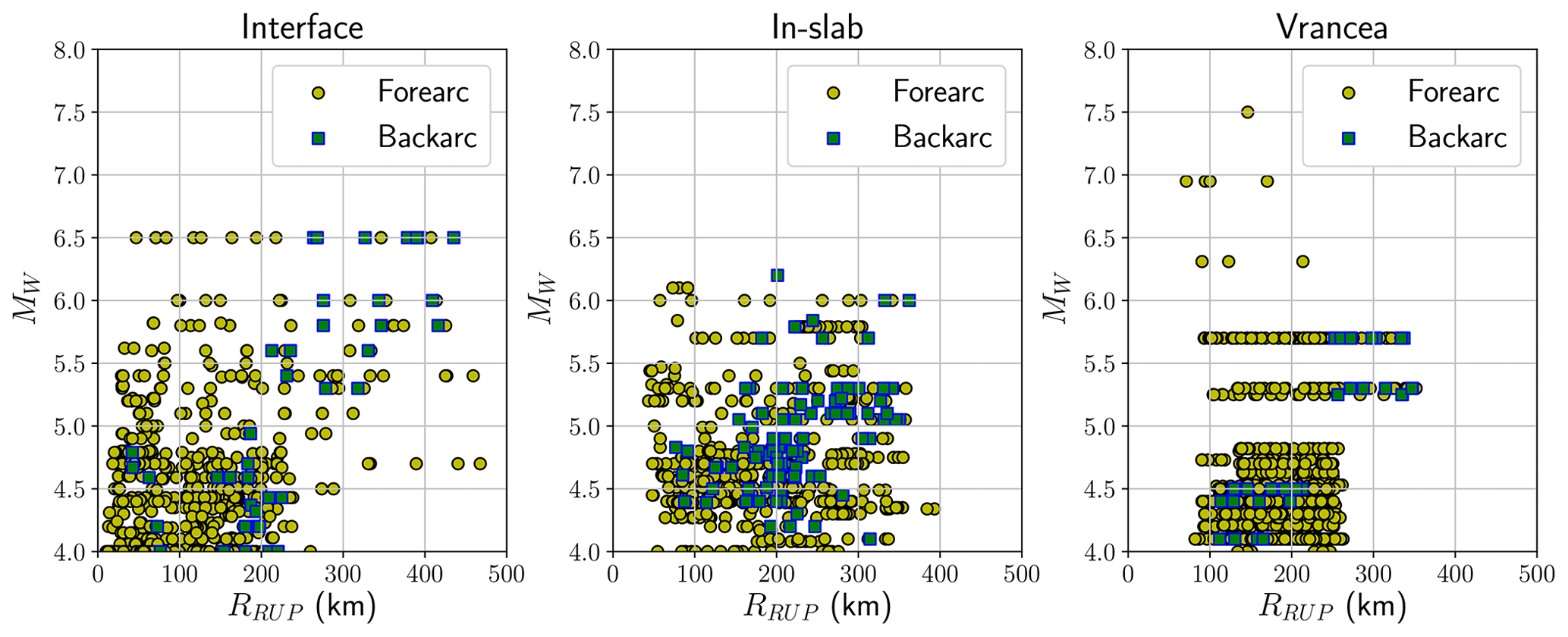
Figure 15Magnitude and distance distributions of the selected records classified according to interface, as in-slab and for the Vrancea deep seismic zone.
The fuzzy classification presented here is a flexible and reproducible approach toward tectonic classification based on limited information. Inevitably as an automatic procedure it is possible for misclassifications to occur or for the classifications to change if some of the underlying data sets change, such as the subduction geometry. There is also subjectivity in the calibration of the antecedent and consequent rules, as well as in the control system itself, and different judgements and rule sets could be made. However, the fuzziness of the system may limit the impact that differences in the shapes of the functions or the logical rules have on the resulting defuzzified classifications, resulting in changes in the classification only in the most ambiguous cases. For example, the interface/in-slab classification will inevitably create a region of ambiguity in the slab if the fuzzy control system depends only on the location of the event. This region of ambiguity would be sensitive to the settings of the antecedent rules. However, if a focal mechanism is available such that an event can be classified confidently as reverse, then the resulting membership shifts more strongly toward interface in this otherwise ambiguous region. For the application to the ESM database here, the number of events considered is relatively small, allowing for the assignments of each earthquake to be verified by inspection. Although it is beyond the scope of this current publication, a comparison of the performance of this fuzzy classification system for subduction earthquakes against labelled classifications found in other subduction ground motion databases such as NGA Subduction would be welcome. Direct comparison may be challenging, however, due to the adoption of different numbers and types of tectonic classes, as well as different models of subduction geometry (not all of which are publicly available). As an indicator of its general versatility, however, the same classifier system was applied successfully for the classification of subduction earthquakes in Papua New Guinea as part of the development of a recent national probabilistic seismic hazard map (Ghasemi et al., 2020).
4.2 Identifying the best suited GMM for use as a backbone GMM
The distribution of records with respect to magnitude and distance shown in Fig. 15 clearly illustrates the possible limitations of attempting to fit a new GMM to the subduction or Vrancea earthquakes. The vast majority of the records fall within the 4.0 5.5 range, with only a couple of well-recorded events above Mw 6.0. The scaling with respect to the magnitudes of significance for hazard from subduction earthquakes (typically Mw≥ 6.5) is virtually unconstrained. Vacareanu et al. (2015) addressed this issue by supplementing their data set with ground motions from well-recorded deep earthquakes in other regions of the globe. This may be a valid approach; however, for ESHM20 we preferred to leverage existing ground motion models that would comply with the quality selection criteria proposed by Bommer et al. (2010) that are constrained by global subduction data, before then attempting a recalibration of the attenuation coefficient of the model based on the Hellenic and Calabrian data. Here, the distance range covered by travel paths from the small-to-moderate-magnitude earthquake ground motions is sufficient to provide some valid inference on ground motion. Although the interface and in-slab record sets contain records from three different subduction zones (Hellenic, Cypriot and Calabrian), further subdivision by zone was not attempted as this would yield too few records from the Calabrian and Cypriot arcs from which to make any inference on attenuation.
The selection of the backbone model is based on a two-step process that first selects a set of candidate models based on quality criteria and then applies likelihood scoring to compare the candidate models against the observed data. We note that the development of the subduction model for ESHM20 was undertaken prior to publication of GMMs from the NGA Subduction project NGA-SUB (Hassani and Atkinson, 2021; Parker et al., 2022; Kuehn et al. 2020; Abrahamson and Gulerce, 2022; Si et al., 2022). The publication of the NGA-SUB models would have inevitably increased the available suite of candidate models for application to the eastern Mediterranean, and we expect this to be an important development step in the next-generation PSHA for Europe. At the time of development, strict application of the Bommer et al. (2010) selection criteria yielded four potential candidate models: Abrahamson et al. (2016) (also known as BC Hydro (2016)), Zhao et al. (2016a, b), Montalva et al. (2017) and Abrahamson et al. (2018). Of these, Montalva et al. (2017) can be considered a regional calibration of the Abrahamson et al. (2016) model using Chilean strong-motion data, while Abrahamson et al. (2018) might be considered more as an intermediate update to the original BC Hydro model using the NGA-SUB database (Bozorgnia and Stewart, 2020), with the more complete update eventually being Abrahamson and Gulerce (2022). We may therefore choose to refer to these as the BC Hydro family of models (Abrahamson et al., 2016; Montalva et al., 2017; Abrahamson et al., 2018). Both Abrahamson et al. (2016) and Abrahamson et al. (2018) propose additional scaling factors to the median ground motions to account for epistemic uncertainty. These are also considered in the comparisons as the high and low branches for the increased and decreased median ground motions respectively.
In the comparisons shown in Fig. 16 we also include the ESHM13 subduction GMM selection (Youngs et al., 1997; Atkinson and Boore, 2003; Zhao et al., 2006; Lin and Lee, 2008) as well as the local GMMs of Vacareanu et al. (2015) and Skarlatoudis et al. (2013) for subduction in-slab events. Although the latter two models are calibrated principally to local data from our regions of interest, they would not be selected for use in ESHM20 owing to their limited period range, limited magnitude range (in the case of Skarlatoudis et al., 2013) and use of site amplification term based on soil class. They are included here, however, to act as models of comparison in the selection process.
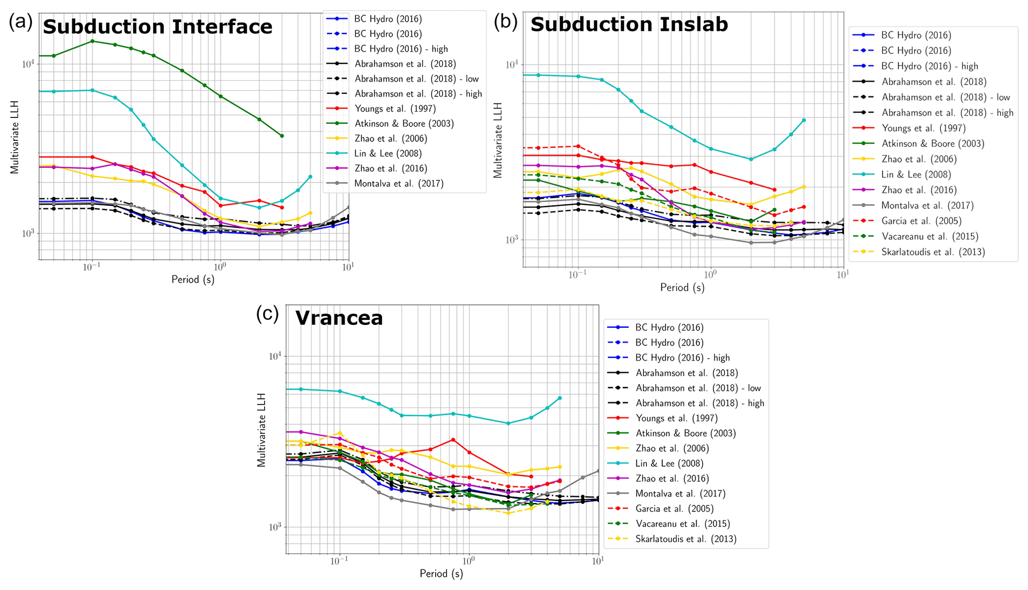
Figure 16Variation in multivariate log-likelihood (ℓℓ) with period for each GMM considered for the subduction interface (a), subduction in-slab (b) and Vrancea (c) regions.
For the likelihood scoring against observed data, we used the multivariate log-likelihood metric of Mak et al. (2017):
where N is the total number of records, p and q are vectors containing the natural logarithms of predicted and observed ground motions respectively, and V is the covariance matrix determined from the between- and within-event standard deviations. Lower log-likelihood scores indicate a closer fit between the model and data, and scoring was undertaken firstly on a period basis. The variation in period for each of the candidate models is shown in Fig. 16 for each of the three data sets: subduction interface, subduction in-slab and Vrancea. Analysis was also undertaken using the earlier log-likelihood scoring method of Scherbaum et al. (2009), but as the ground motion records are relatively well balanced across the events in the data, the trends were found to be nearly identical to those determined using from Mak et al. (2017), so only the latter are shown here for brevity.
Figure 16 demonstrates that in all three cases each one of the candidate models has a lower likelihood score across the full period range than any of the ESHM13 model selection. At longer periods, Zhao et al. (2016a, b) may give a slightly improved fit when compared to the Zhao et al. (2006) predecessor, but the differences are small and a slight deterioration is seen at short periods. For the subduction interface earthquakes all of the BC Hydro family are comparable, with Abrahamson et al. (2018) improving slightly on Abrahamson et al. (2016) at intermediate periods and Montalva et al. (2017) slightly poorer in the same range. Differences are nearly negligible, however. The lower adjusted branches appear to give a lower score than the higher adjusted branches or unadjusted branches, which may imply a regional tendency toward lower stress drop than the global models. However, this latter observation should be interpreted with caution given the magnitude range considered in the data, the high proportion of Mw values converted from local magnitude ML and body wave magnitude mb in this region and range, and the possibility of systematic differences in path and site effects. For the subduction in-slab events the trends are similar, with the noteworthy exception that Montalva et al. (2017) appears to give a significantly lower score in the 0.5 to 4 s period range than the other models in the BC Hydro family. The locally fit Skarlatoudis et al. (2013) model performs comparably to the BC Hydro models for in-slab earthquakes, which is not surprising given the large overlap in the original fitting data set and the test data set. That there is no improvement in fit for using the locally calibrated model compared to the global model strengthens the case for adopting the global models here. For Vrancea, the Vacareanu et al. (2015) is shown to give slightly lower values than the BC Hydro models at very short periods (T < 0.2 s), but the results are comparable for the rest of the spectrum. Once again, Montalva et al. (2017) surprises with lower values across much of the period range, even more so than Vacareanu et al. (2015).
From the likelihood scoring of the GMMs it is evident that any of the BC Hydro family could be considered as a possible backbone model. Montalva et al. (2017) produced less than the original BC Hydro for the in-slab and Vrancea cases, which is interesting, but as it is a regional calibration of Abrahamson et al. (2016) it is not necessarily a good basis as a backbone model as further adjustments will be undertaken here. A case could also be made for adopting Abrahamson et al. (2018) as the backbone; however, not only does this model lack a forearc/backarc scaling term, it also does not provide a significant improvement in fit with respect to the Abrahamson et al. (2016) model, with the possible exception of short-period in-slab events. The absence of a forearc/backarc scaling term is problematic as differences in backarc attenuation do seem to be present in the model of data residual values and in previous studies of attenuation in both the Carpathian region (Vacareanu et al., 2015) and the Hellenic Arc (Skarlatoudis et al., 2013). We therefore opt to adopt the original Abrahamson et al. (2016) BC Hydro model as the backbone GMM for use in the subduction and deep seismicity logic trees.
4.3 Calibration of the model and definition of the backbone logic tree
The ground motion observations for subduction and deep seismicity earthquakes shown in Fig. 15 indicate that while the magnitude range of the data may be limited, particularly with respect to larger magnitudes, the distance range is well covered. Inspection of the site information at these same stations revealed that most stations in the data set lacked a measured VS30, and as magnitudes are small very few if any records would likely show soil nonlinearity. Given these limitations, in contrast to Montalva et al. (2017), we do not attempt a full regression of the BC Hydro model on the new data but instead choose only to recalibrate the anelastic attenuation term of the model:
and fSITE(PGA1100,VS30) are the magnitude scaling, geometric spreading, anelastic attenuation and site amplification term for an earthquake of magnitude Mw recorded at a site of distance R km from the source on a site condition VS30 (m s−1). θ4ΔC1 is a term applied to large magnitude to account for epistemic uncertainty in the magnitude scaling, while θ1 is the regional stress coefficient. Note that for interface earthquakes the nearest distance to the rupture plane RRUP is used, while for in-slab earthquakes the hypocentral distance is preferred (RHYPO). fFABA(R) is the forearc/backarc scaling term, which is discussed in more detail in the following section. For in-slab earthquakes an additional source depth scaling term fdepth(Zh) is included, where Zh is the hypocentral depth in kilometres, and additional coefficients are added to both the stress term θ10FE and to the geometric spreading term to reflect differences for in-slab earthquakes (indicated when FE=1, otherwise FE=0). An additional epistemic uncertainty scaling factor Δμ=0.2 is suggested by the authors
As we are aiming to calibrate only the anelastic attenuation part of the model, our interest is in only fa(R) and where . To calibrate the coefficients for these terms we retrieve between- and within-event residuals (δB and δW) for the observations with respect to the model in which fa(R)=0. The trends in δW are inspected with each period, and a linear model is fit such that the slope θ6 is calculated and constrained to be ≤ 0.0. The variation in fitted θ6 with spectral period is shown in Fig. 17 for the interface ground motions (black) and in-slab ground motions (red). The attenuation terms from the two data sets show divergent behaviour at short periods, with slower attenuation for in-slab earthquakes than interface earthquakes, gradually converging at T≥1.0 s. As a point of comparison, we also show the anelastic attenuation coefficients from several other regions of the globe, as presented by Abrahamson et al. (2018) in their exploration of regional variability of anelastic attenuation implied by the NGA-SUB data set. We also include the terms from Vacareanu et al. (2015) and from Montalva et al. (2017). These regional differences are similarly divergent, with certain regions aligning more closely with the slower attenuation in-slab data set (e.g., Central America, Taiwan, Romania forearc) and others with the faster attenuating interface data set (e.g., New Zealand, South America, Cascadia, Japan).
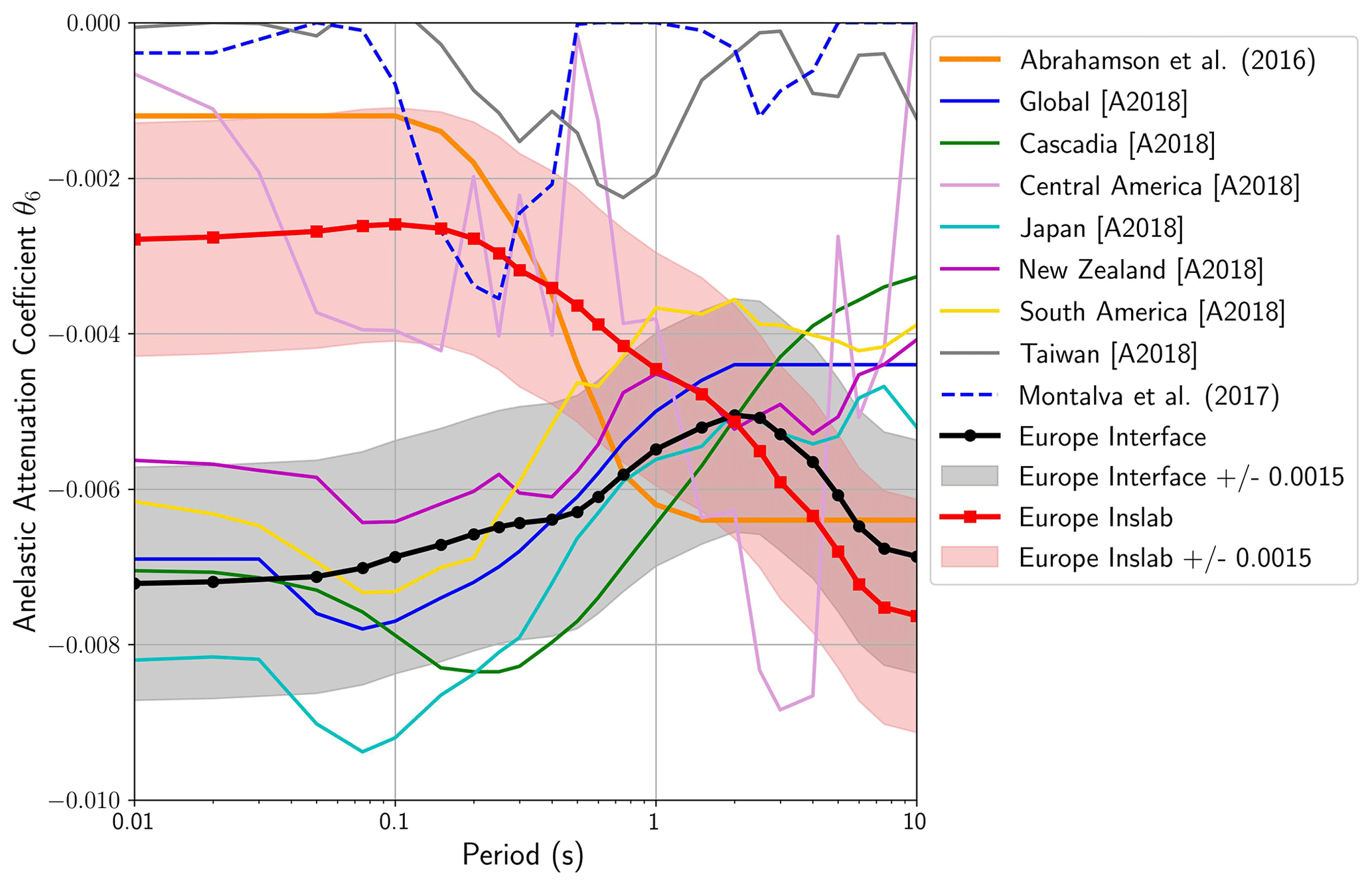
Figure 17Variation in the anelastic attenuation coefficient θ6 with period for the observed European subduction interface (solid black line) and in-slab (solid red line) earthquake data, with the proposed epistemic uncertainty of ±0.0015 shown in grey and pink shaded regions respectively. Anelastic attenuation coefficients from different regions across the globe calibrated by Abrahamson et al. (2018) are shown (with labels [A2018]) along with that of Montalva et al. (2017).
While the calibrated attenuation coefficients θ6 are set for the interface and the in-slab earthquakes, Fig. 17 demonstrates that there exists clear region-to-region variability. In order to construct the backbone GMM logic tree, we need to account for epistemic uncertainty in the anelastic attenuation and calibrate specific adjustment factors to represent this. The region-to-region variability in the anelastic attenuation term explored by Abrahamson et al. (2018) (A2018 in Fig. 17), while not exactly comparable to our backbone model, does provide insights that can help us define scaling factors. In this case we find that adjustments to the θ6 term of ±0.0015 are adequate to envelope region-to-region variability for the two trends in the residuals. We therefore define three branches for the anelastic attenuation model: θ6−0.0015 (fast), θ6+0 (central) and θ6+0.0015 (slow). Although there is no specific distribution represented by these terms, we nevertheless opt to treat them consistently with the attenuation terms in the shallow-crustal-seismicity models and assign them weights representing the three-point Gaussian approximation of Miller and Rice (1983), namely 0.167, 0.666 and 0.167 respectively.
The results for the Vrancea data set are not shown here, as the anelastic attenuation term appeared to show weakly positive θ6 trends, which are then constrained to θ6=0 in the regressions. Given this unusual behaviour it may not be entirely surprising that it was the Montalva et al. (2017) GMM that produced a significantly lower model than the Abrahamson et al. (2016) model for Vrancea, as it has the weakest anelastic attenuation term among the subduction GMMs compared in Fig. 16. Analysis by Manea et al. (2022) of a more extensive set of ground motion records from Romania, which was undertaken after the construction of the ESHM20 GMMs, confirmed the appearance of the very slow attenuation at short periods, particularly for sites in the forearc region (to the east and south of the Carpathian mountain belt). This region is evidently complex and further analysis is needed to refine and calibrate the ground motion models, particularly considering the study by Manea et al. (2022). Though there is a case for adopting or assigning heavier weights to slower attenuation branches, we were unsure whether the data available to us were sufficiently compelling to do so. Instead, we adopt the in-slab backbone GMM and its calibrated attenuation adjustments but assign slightly higher weights to the upper and lower branches than the middle branch. Finally, the three branches (fast, central and slow) are assigned weights of 0.2, 0.6 and 0.2 respectively.
While attenuation and its uncertainty are clearly important for non-crustal seismicity, stress parameter uncertainty and large-magnitude scaling have also been identified as critical areas of epistemic uncertainty in subduction and deep earthquake GMMs (Abrahamson et al., 2016, 2018; Gregor et al., 2022). In the original BC Hydro model, Abrahamson et al. (2016) proposed a set of adjustments to be applied at large magnitudes in order to account for uncertainty in the break point of magnitude scaling in the GMM given the limited number of very large earthquakes in the data set – an issue that was explored in more depth in the NGA-SUB project (e.g., Campbell, 2020; Kuehn et al., 2020; Abrahamson and Gulerce, 2022). Without records from large-magnitude earthquakes (and only very few from moderate-magnitude earthquakes), our observations do not give us a basis for recalibrating these adjustments; however, as they apply principally to very large Mw≥8 earthquakes, such factors will have a negligible impact on the PSHA results for the probabilities of interest in ESHM20, owing to the low annual rate of occurrence for these events. More relevant is the epistemic uncertainty in the stress term and the statistical uncertainty in the models. Abrahamson et al. (2018) explored this in more detail and proposed a median ground motion adjustment factor ε⋅σμ, which is fixed to ±0.3 for interface events and is period-dependent for in-slab events changing from ±0.5 at short periods to ±0.3 at longer periods. The factors are defined such that region-to-region variability in the stress term is enveloped by , where ε in this case is assumed to be 1.65. To apply the factors in our logic tree, we retrieve σμ from the factors given (taking ε=1.65) and then map this into our logic tree branch set assuming N(0,σμ). As this epistemic uncertainty is determined solely from the stress term of the model (θ1) it is independent of magnitude and distance scaling. We can therefore apply it alongside the attenuation adjustment factors without the risk of double-counting epistemic uncertainty.
Our final set of GMM logic trees for application to subduction interface, subduction in-slab and Vrancea deep seismicity is shown in Fig. 18, alongside the distribution of ground motions with distance and period for interface and in-slab earthquakes in Figs. 19 and 20 respectively. Each region requires a different logic tree, the subduction interface and subduction in-slab models applying different backbone GMMs and θ6 values, while for Vrancea we apply the in-slab GMM but with higher weights on the outer attenuation branches. In the final application the distribution of σμ is mapped to five branches using the approach of Miller and Rice (1983), but the attenuation epistemic uncertainty is kept to just the three (fast, centre and slow) branches with their aforementioned weights.
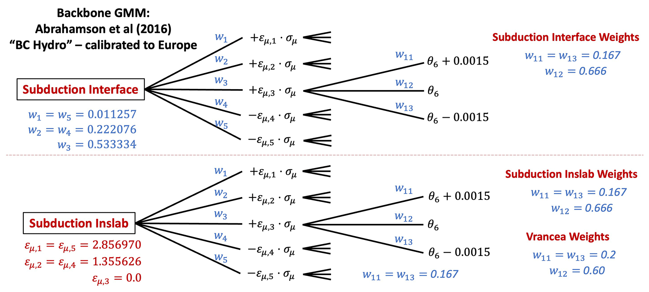
Figure 18Final ESHM20 scaled-backbone GMM logic tree for subduction interface, subduction in-slab regions and the Vrancea deep seismic zone.
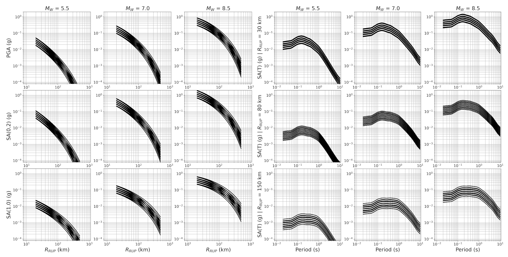
Figure 19As Figs. 3 and 7 for the subduction interface scaled-backbone GMM logic tree. Magnitudes considered at Mw 5.5, 7.0 and 8.5 (columns) and distances RRUP= 30, 80 and 150 km respectively. Sites are assumed to be forearc with VS30 800 m s−1.
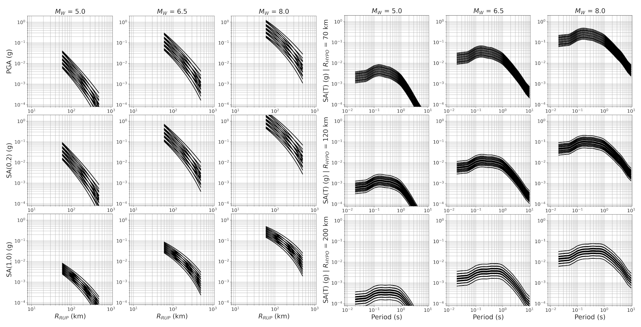
Figure 20As Fig. 19 but for the subduction in-slab and Vrancea deep zone scaled-backbone GMM logic tree. Magnitudes considered at Mw 5.0, 6.5 and 8.0 (columns) and distances RHYPO= 70, 120 and 200 km respectively. Sites are assumed to be forearc with VS30 800 m s−1.
The development of the backbone GMM for subduction and deep seismicity ground motions has principally focused on characterising epistemic= uncertainty in the median ground motion for the reference rock condition of VS30 800 m s−1. Both the aleatory variability and the site response have an influence on the seismic hazard and on the risk calculations for ESRM20. In both cases we lack the data to attempt to recalibrate the existing terms in the models, so for the ESHM20 calculations the aleatory variability term in the subduction GMM is executed unadjusted, while for the site response component of the ESRM20 we use the model with the topographically inferred VS30 rather than attempt to recalibrate the site amplification as a function of slope and geology (Weatherill et al., 2023). The possibility to run a partially non-ergodic form of the model is supported in the OpenQuake implementation. In the original BC Hydro model, a period-independent total ergodic aleatory variability of σT=0.74 is given; however, applications of the GMM to the site-specific PSHA project in the United States suggested that a period-independent single-station σSS of 0.60 could be used. From this we infer a site-to-site variability of ϕS2S=0.43, which can be removed from σT if the user chooses to do so for site-specific analysis.
4.4 Forearc/backarc scaling
4.4.1 Identification and calibration of forearc/backarc scaling
One of the most significant changes in subduction ground motion modelling that separates the earlier subduction GMMs such as those used in ESHM13 from the current state of the art is the introduction of terms to account for differences in attenuation between travel paths that are predominantly forearc and those that are predominantly backarc. This is evident in Eqs. (9) and (10) by the forearc/backarc scaling term fFABA, which was introduced by Abrahamson et al. (2016) for subduction ground motions such that
where FEVENT=1 for in-slab events and 0 for interface, and FFABA=1 if the site is located in the subduction backarc and 0 otherwise.
More extensive regional analysis in the later NGA-SUB GMMs showed that these forearc/backarc scaling differences were not present in all subduction regions (Parker et al., 2022; Kuehn et al. 2020; Abrahamson and Gulerce, 2022); however, in some regions the national strong-motion networks lacked sufficient stations in the backarc regions to identify differences. Variations in attenuation depending on the source to station azimuth have also been well observed in earthquakes originating in the Vrancea deep seismic zone (e.g., Ivan et al., 1998; Sokolov et al., 2008), and recent GMMs in this region have introduced forearc/backarc adjustments (Vacareanu et al., 2015) or even defined along-arc adjustments (Manea et al., 2022). In the development of the subduction and deep seismicity GMMs for ESHM20 the issue of forearc/backarc scaling must be addressed, but several steps are needed in the process: (1) define the forearc/backarc regions and classification of records, (2) determine whether differences in ground motion attenuation are present, (3) determine whether adjustments to the existing scaling terms are necessary and could be achieved with the available data.
For our analysis we have defined the boundary between forearc and backarc based on the subduction geometry (inferred from Slab 2.0) and relative position of the volcanic front. These boundaries are shown in Fig. 21 as volcanic fronts. For the Hellenic Arc the initial boundary is placed in the southern Aegean Sea beginning with the volcanic southern Cyclades islands, before then extending westward to Methana (southern Greece) and eastward through the Dodecanese islands to come onshore close to the Datça Peninsula in southern Türkiye. This line joins the main southern Aegean volcanic chain, which we then continue to extend northwestward through southern Greece into Albania and eastward through southern Türkiye running in line with the subduction geometry. A similar approach is taken in the Calabrian Arc, and while the volcanism present in the southern Tyrrhenian Sea is different in nature to that of a purely subduction-driven volcanic front, for the purposes of attenuation it is used as a reference point. Here the volcanic front passes through the Aeolian Islands and follows the azimuth of the Calabrian subduction westward to cross northern Sicily and northeastward to come onshore in southern Campania. Though the volcanic fronts are delineated by judgement, they are also contrasted against maps of heat flow such that regions of higher heat flow are predominantly found in the backarc regions. For Vrancea we retained a previous delineation used by Weatherill and Danciu (2018), which itself followed that of Vacareanu et al. (2015), who delineated the boundary closely following the watershed of the Carpathian mountain belt. This places Hungary and northwestern Romania in the backarc region, while most of the Danube basin, Bulgaria, eastern Romania and Moldova are found in the forearc.
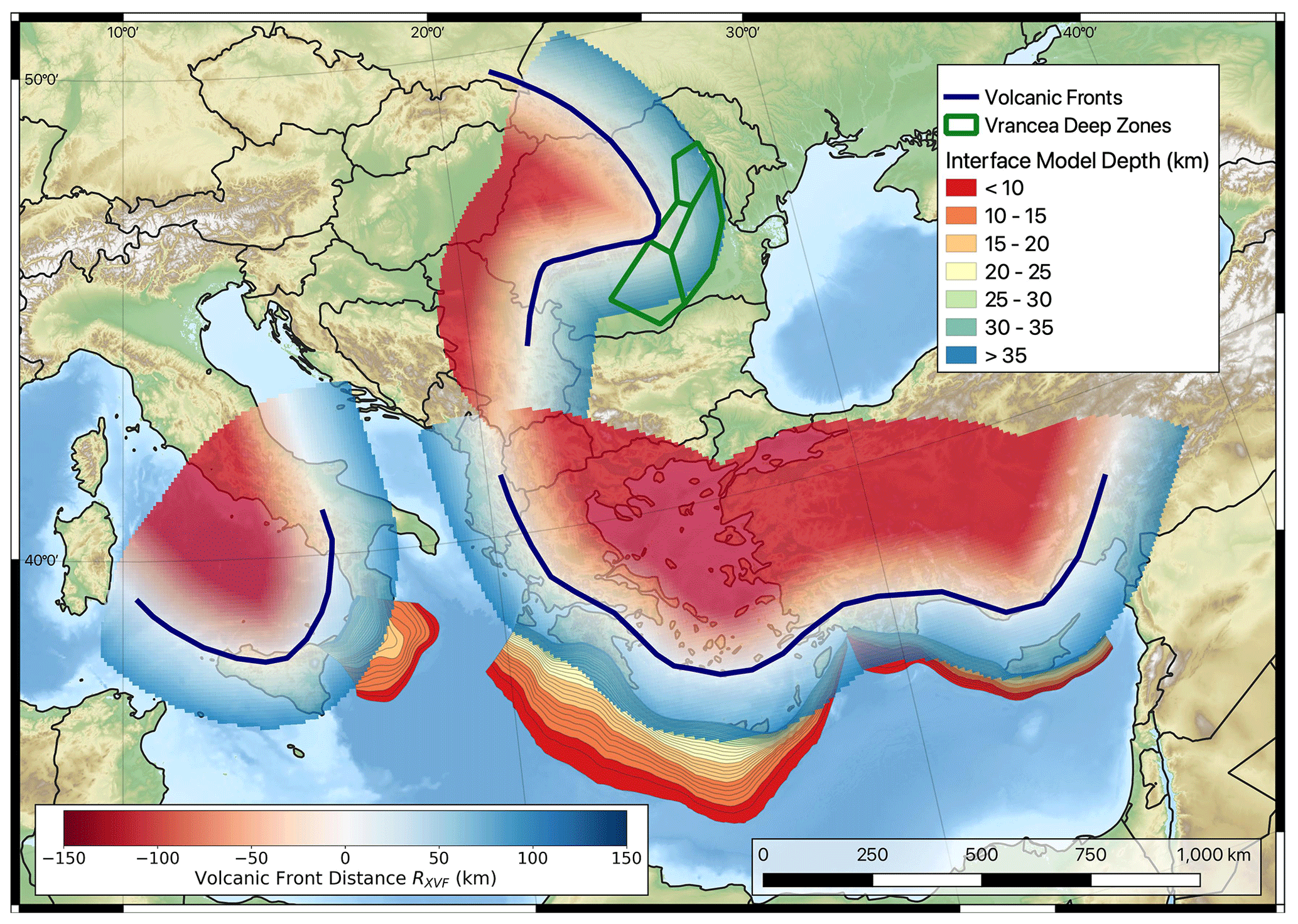
Figure 21Definition of the subduction interfaces, the volcanic fronts (dark blue lines), and Vrancea deep source zones (green), along with variation in RXVF used for ESHM20. Backarc regions are shown in red and forearc regions in blue. Figure adapted from Danciu et al. (2021).
With the boundaries delineated, the records in our ground motion databases are classified either as forearc or backarc, as shown in Fig. 21. As our data come predominantly from small- to moderate-magnitude events, the proportion of usable strong-motion records in the backarc regions is generally low, particularly for interface events. To determine if differences in attenuation between forearc and backarc records are present, we retrieve the within-event residual with respect to the Abrahamson et al. (2018) GMM, which itself does not include fFABA. For sites with RRUP≥120 km, we compare the mean and standard deviations of δW for the forearc residuals with those for the backarc residuals and apply a two-sided Kolmogorov–Smirnov test to indicate the significance of the hypothesis that both are drawn from the same distribution. This is applied to each of the three data sets and for each period. We found that for interface earthquakes the null hypothesis that the backarc residuals are drawn from the same distribution as the forearc residuals cannot be rejected at probability level p= 0.05. For the in-slab and Vrancea databases, the distributions are significantly different (p≪0.05) for spectral periods less than 0.75 s, indicating clear evidence of a difference in attenuation scaling between forearc and backarc sites. The period range of forearc/backarc scaling influence aligns well with the period range for which fFABA in the Abrahamson et al. (2016) is significant. Undertaking the same analysis of δW using our backbone GMM, which included fFABA but with anelastic attenuation calibrated as described previously, we find that the differences in the two residual distributions are greatly reduced. The data clearly demonstrate that a backarc scaling is present. However, while further calibration of fFABA to the European data might have been desirable, the volume of data from records with predominantly backarc travel paths was insufficient to clearly separate the differences in general anelastic attenuation from those of the backarc scaling. We therefore retained fFABA unadjusted from Abrahamson et al. (2016) and calibrated only θ6 accordingly. This does not discard the possibility that if fFABA does not fully capture the differences in backarc scaling in our data, then some of this bias may propagate into the calibrated anelastic attenuation term.
4.4.2 Implementing forearc/backarc scaling in regional PSHA
Of the subduction GMMs considered so far that have included fFABA, this term has been modelled as a property of the site and hence applied when the site is in the backarc with respect to the subduction zone and not applied when in the forearc. Yet the phenomenon it is modelling is related to the material through which the wave has travelled and not the site itself. This binary classification, while practical, can be problematic. Other GMMs have adopted more path-dependent properties to capture similar variation in attenuation that capture these effects via terms such as path distance through the backarc or through volcanic zones (e.g., Skarlatoudis et al., 2013; Zhao et al., 2016b, c; Campbell et al., 2022). For regional-scale PSHA such as the ESHM20, the binary switch from forearc site to backarc site across the volcanic front results in sudden cliff edge changes in seismic hazard (Weatherill and Danciu, 2018).
Replacement of FFABA with a path-through-backarc distance term in the GMM may be preferable from a pure physical perspective, but such a term requires that the PSHA software trace the path between the source and site to measure the proportion through the backarc. The path tracing is not a trivial calculation when considering tens of thousands of sources and thousands of sites, as we are in the ESHM20, and would incur substantial computational cost. This option was not available to us in the current version of the OpenQuake-engine software. Instead, we attempt to achieve a smoother transition between forearc and backarc attenuation regime by turning FFABA into a continuous function that varies over source-to-site distance. To do this we define for each site the distance to the line of the nearest volcanic front RXVF, which takes a positive value on the forearc side and negative on the backarc. This is a static property of each site, but it varies as a continuous value as one moves across the volcanic front (shown in Fig. 21). We then relate RXVF to FFABA via a taper function that is applied over a distance range. The total number of backarc records are limited and the proportion of those that fall close to the volcanic front even more so. We cannot therefore test the influence of the tapering function against data, but rather we compared different tapering functional forms by inspection of the attenuation trends in the resulting GMMs. The preferred option is a so-called “S function”:
where a and b are fixed values that define the distance range over which the taper is applied. We set these to −100 and 100 km respectively, meaning that the transition from full forearc to full backarc attenuation regime occurs over a 200 km distance centred on the volcanic front. In the OpenQuake implementation of the GMM, the choice of taper function and the controlling values is available to the user, meaning that others could add alternative models as epistemic uncertainties, although we choose not to consider epistemic uncertainty on this function in the ESHM20. In the final model RXVF is calculated for all sites within 500 km of the subduction interface (in the case of the Hellenic, Cypriot and Calabrian arcs) or within 500 km of the surface projection of the Vrancea deep seismogenic sources (also Fig. 21). This covers the maximum integration distance used for the subduction GMMs in the PSHA calculation. For the Gibraltar subduction we do not consider any sites to be backarc. For the Mediterranean subduction zones the distances for sites in the Ionian Sea are consistent with one another, but a small incoherence is visible near the northern border of North Macedonia, which would be classified as forearc with respect to the Vrancea zone but as backarc with respect to the Hellenic Arc. This is undesirable, but this incoherence occurs at distances of more than 400 km from either deep source, in a region where shallow-crustal-seismicity dominates the hazard. The impact of this incoherence on the seismic hazard was found to be completely negligible.
4.5 The next generation of subduction and deep seismicity GMMs for Europe
At several points throughout this section is has been noted that the efforts to develop the backbone GMM logic tree for non-crustal earthquakes preceded the publication of the NGA Subduction GMMs. Much like their NGA West and NGA East counterparts, the NGA Subduction GMMs are transformative in how they approach problems of regionalisation; uncertainty (epistemic and aleatory); and source, path and site scaling for subduction earthquake hazard. The implications of this for hazard in Europe need to be understood, and a more extensive analysis of the models and their comparison to ground motions in the eastern Mediterranean and Romania would be an important starting point for subduction GMMs in Europe. No ground motions from Europe were included in the NGA Subduction database (Bozorgnia and Stewart, 2020), yet the volume of records from non-crustal seismicity in Europe is growing (Manea et al., 2022; Luzi et al., 2020) and the site characterisation of recording stations improving. While we are unlikely to witness many large subduction or deep seismicity earthquakes in Europe within the following few years, there remains scope to use this growing body of data to attempt to calibrate certain parameters of the NGA Subduction GMMs for application to the Hellenic Arc and to explore the issue of regionalisation in more detail. Likewise, as discussed in the following section, non-ergodic GMMs are likely to play a significantly greater role in the next-generation ESHM than was possible for ESHM20. The implementation issue of path tracing inside the PSHA calculation software will inevitably need to be addressed in the PSHA software, and if supported in future versions of OpenQuake then this opens up the possibility to move beyond the forearc/backarc scaling undertaken here and into more flexible and physically sound characterisation of travel path differences.
The development of the ESHM20 and the growth of data sets such as ESM provided us an opportunity to rethink how to approach the question of ground motion characterisation and its epistemic uncertainty in PSHA. While the concept of the backbone GMM logic tree has gradually developed in the specific PSHA during the last decade, there were few precedents for its application at a large regional scale, particularly one that encompasses a diversity of different tectonic domains. Throughout the process it has been tempting to push the modelling concepts even further, to capture as much of the nuance as we are able and to explore uncertainties wherever possible. At the same time, however, the practicality of implementation and execution is a key issue, and we have inevitably had to adapt ideas to the computational framework that we had available to us and to allow the calculations to run in a reasonable time without the need for excessive computational resources. In this concluding section of the paper, we will take the opportunity to reflect on what has been successful in this approach, what were the limitations and, finally, in what directions we would expect to see the next generation of GMMs for PSHA in Europe developing.
5.1 A new framework for ground motion modelling and integration of data
Notwithstanding whether every decision made here in constructing the GMM logic tree is the right one, the development of the regionalised scaled-backbone GMM logic represents a change of framework for how data should inform the modelling process. We are no longer aiming to find the best models from those available in the literature, but rather we begin in our process with the best fitting model (be it derived directly from the data or simply best suited to the data and/or context) and aim to translate our knowledge of the seismological properties of a region into a distribution of expected ground motions centred on our best fitting model. This allows us to ensure that the branches in the logic tree fulfil the mutually exclusive and collectively exhaustive criterion for epistemic uncertainty characterisation (Bommer and Scherbaum, 2008). By introducing the regionalisation concept, we allow the centre of this distribution to change according to the trends reflected in our underlying data and the variance to decrease in places where a high volume of data may give us greater confidence in the trends we are seeing. Conversely the variance increases where we have little or no data, which is also a fundamental requirement of epistemic uncertainty characterisation. This change in framework means that the model can be continually (or at least frequently) adapted as new ground motion observations are fed in, and this can directly influence the hazard models for a region as the centre of the logic tree may change in accordance with the observations and the variance is reduced. The framework adopted here could have already been more adaptable to work in this fashion, and in many cases, we imposed constraints ourselves to smooth out local-scale variability that may be over-fitting to the limited data and to retain the practicality of implementation at the European scale given the tools and resources available. Such constraints may be gradually relaxed if one wished to apply this same framework at a local scale and capture more of the local seismological characteristics.
The exact manner in which one may wish to adapt the framework to local data can in itself be flexible. The original distributions of δc3 and δL2Ll emerge from the random effects regression, and as we are using open data it is entirely possible for the regression to be rerun as new data emerge. This also lends itself perfectly to a Bayesian updating framework similar to that proposed by Stafford (2019), in which the current model, its random effects and their uncertainties form prior distributions that can be updated with new data, potentially in an operational framework. This has already been attempted for France using the Résif data set (Kotha and Traversa, 2024). These processes would, of course, result in small but potentially noticeable changes to the fixed effects in the GMM, which may or may not be desirable depending on the application. However, while updating of the model in the formal sense may be useful for successive generations of European-scale applications, through the data-informed decisions and/or adaptations of the model that we introduced for the special case regions we also showed how it was possible to modify the distribution of ground motions within the same framework without needing recalculation of the GMM. This is, above everything else, the intent of the model for future applications. We may be able to adapt the model, calibrate it to local data and incorporate new facets non-necessarily constrained by data, without necessarily requiring a new approach. This can help ensure more stability in the seismic hazard in regions where few new data have been assimilated (or few earthquakes occurred) from one generation to the next, while at the same time ensuring that inferences about the underlying seismological properties that may be gained from subsequent seismic observations can inform the calibration of the GMM logic tree in regions where these new observations are available.
As a small note, although we have embraced the scaled-backbone GMM logic tree concept fully in the implementation for ESHM20, this same framework could easily accommodate a hybrid multi-model and scaled-backbone approach too. This would entail selecting multiple backbone models for use in a region that may reflect different underlying modelling choices or physical constraints (i.e., model-to-model variability) while at the same time applying scaling factors to account for within-model uncertainty. The recent 2022 National Seismic Hazard Model for New Zealand successfully adopted such an approach (Bradley et al., 2023). The obvious cost would be the increase in the number of logic tree branches, but if this were acceptable to the modeller then this could be implemented in application and still be consistent with the current framework.
5.2 Limitations
The framework for the regionalised scaled-backbone GMM logic tree might itself represent a sustainable pathway for continual refinement in future models; however, the exact characteristics of the GMM logic tree adopted for ESHM20 will inevitably contain decisions or features that may be improved and/or reconsidered in the future. Some of these arise from practical limitations of the tools and/or data, while others may reflect the need for further research efforts. One of the largest changes between the current GMM logic tree and that of ESHM13 is that for the tectonically stable non-cratonic regions of northern and western Europe we no longer incorporate GMMs from the stable cratonic regions. Instead of building a logic tree that selects one or more CEUS GMMs and assigns them a minority weight, we assumed that where we lacked the data the distribution of tectonic-locality uncertainty and residual-attenuation uncertainty implied by the full region-to-region variability in the ESM data set was sufficiently representative. We still retain branches for high stress drop and slow attenuation, but they receive a lower weighting than the CEUS GMMs did for the ESHM13 logic tree and are also balanced by branches for lower stress drop and faster attenuation. This is more aligned with recent PSHA models in France (Drouet et al., 2020), Germany (Grünthal et al., 2018) and other lower-seismicity regions (e.g., Mosca et al., 2022), where the logic trees have shifted more toward representation by active shallow-crustal-seismicity GMMs, albeit in some cases with adjustments to capture the possibility of higher stress drop. The exclusion of the CEUS models from the logic tree has a notable impact on the seismic hazard both in ESHM20 and in the national models, significantly reducing the mean and median seismic hazard. The assumption of representativeness in region-to-region variability is a somewhat strong one, and the adaptations made for western Europe by applying the slow-attenuation cluster region over a large area reflect a change of view of the modellers regarding the assumption. The confirmation of a difference in the regional attenuation for parts of western Europe did result from new data (Kotha, 2020); however, the decision to connect such differences to geological age meant that we extended this to other regions by virtue of this predictor rather than based on data. Effectively, we changed our original assumptions. We believe this approach to be rational and consistent with science, but we did not extend it across the entirety of the tectonically stable non-cratonic region of Europe. We cannot say whether this was right or wrong, and we would look to new data from weak-motion records to perhaps give us further insights here.
In opening up the question of representativeness of the modelled region-to-region variability, we should also not overlook that in deriving the model in the first place there are several other assumptions or important factors that can influence the outcome. The first assumption is, of course, the regionalisation itself, which is based on an interpretation of geology and tectonics that may not itself reflect variations in the seismological properties that most affect ground motion scaling and attenuation. Other regionalisations could also be considered and may yield different, though not necessarily incompatible, results. The adoption of separate regionalisations for δL2Ll and δc3, while initially founded on a reasonable premise that factors controlling the two terms may be different, resulted in limitations later in the process when reducing the number of regions. With hindsight, adopting a common regionalisation for both may have more easily accommodated the possibility of applying clustering over both distributions, making it possible to identify common regions of lower/higher stress parameter and slower/faster attenuation. The question of regionalisation could be revisited in future if one does not adopt directly full-scale non-ergodic models based on regular grids.
Another factor that may have potential influence on regionalisation, and one that requires further investigation and refinement, is variability in the definition of the magnitude. The ESM flatfile did not contain a harmonised Mw for all the events, and therefore the magnitudes used in the regression were assigned from the harmonised European-Mediterranean Earthquake Catalogue, which had been shown to reduce the between-event variability compared to the use of the heterogeneous magnitudes in the original ESM flatfile (Bindi et al., 2019). For many earthquakes with M < 5.0, moment magnitudes were either taken directly from different local moment tensor databases (sometimes without adjustment) or were converted from other magnitude scales by locally or regionally calibrated conversion equations (Grünthal and Wahlström, 2012). As EMEC is itself compiled on a region-by-region basis, it is possible for region-to-region variability in the magnitude definition to propagate into the tectonic-locality variability of the regression, particularly for regions where the seismicity used to calibrate δL2Ll is low magnitude. This is, regrettably, unavoidable but demonstrates the need for closer integration between the catalogue compilation process and the ground motion model development to identify where regional biases in magnitude estimation may be manifest in the regional variability of the GMM. This too is another reason why we did not attempt to fully regionalise δL2Ll for ESHM20, but future models will likely attempt to do so and should be aware of this potential bias.
The next major limitation is one that was already highlighted by Kotha et al. (2022) and that relates to the large-magnitude and near-fault scaling. While the ESM data set boasts a significant increase in the number of ground motion records compared to its predecessor, this increase has come mostly from small events. For Mw≥6.0 generally it is the 2012 Emilia-Romagna sequence and the 2016 central Italy earthquake sequence that contribute the largest volume of records from large-magnitude shallow-crustal-seismicity events. For larger earthquakes with Mw≥ 7.0, the database is dominated by a few well-recorded large Turkish earthquakes (e.g., Izmit, 1999; Duzce, 1999; Van, 2011). These are not necessarily rich in near-source records, and it required careful scrutiny of the Kotha et al. (2020) model and comparison against the subsequent NESS data sets to identify the apparent oversaturation issue that was addressed by reducing the breakpoint in magnitude scaling Mh from Mw 6.2 to Mw 5.7 in the Kotha et al. (2022). The ESHM20 backbone model (along with most other European models) has not introduced near-fault scaling terms to predict features such as hanging-wall amplification or directivity, which were calibrated largely from inferences using ground motion simulations (in addition to some seismological theory e.g., Abrahamson et al., 2014; Chiou and Youngs, 2014). This does not mean that such factors are not predicted per se, but rather that they form part of the aleatory uncertainty of the model. Further refinement of the large-magnitude scaling calibration of the model, as well as the potential introduction of terms to better capture near-source phenomena, would require expansion of the analysis to incorporate records from large-magnitude earthquakes in other regions of the globe (such as NESS), physics-based ground motion simulations or, most likely, both. These will be discussed among the longer-term developments in due course, but they will inevitably form critical areas of research in the coming generations of seismic hazard models.
5.3 Developments for the future
The European Seismic Hazard Model (ESHM) has a relevant role in steering the evolution of seismic hazards across Europe. While its overriding aims will be to produce a pan-European view of seismic hazards to be used by stakeholders from various sectors, its development can help to focus where and how research in engineering and seismology can be integrated into seismic hazard assessment. We can broadly categorise developments for the future as near-term/local or long term. The former refers to specific improvements or issues that could be explored and integrated within the current frameworks and tools and may be of relevance for new national PSHA models or interim updates to the ESHM in a time frame of months to years. The latter reflect the larger-scale trends in ground motion modelling that we see evolving in both research and application across the globe, which may not be immediately integrated into current practice but should reflect the directions that it may move in over the timescale of years to decades.
5.3.1 Refinements and near-term improvements
Many of the short-term refinements and improvements follow from the limitations highlighted earlier in this section and throughout this paper. These include the following.
Integration of recent ground motion data and revision of the backbone models. This development would integrate recent ground motion data assimilated into ESM after the compilation of the flatfile by Lanzano et al. (2019), potentially including other ground motion records from around Europe that would comply with the quality criteria set by ESM. It would require updating the fixed and random effects, which could be undertaken in a Bayesian framework (e.g., Stafford, 2019). Revisions to the regionalisation, or even support for different regionalisations, could be integrated if necessary, particularly where data are unevenly distributed across a single region. Depending on the geographical scale of the application and the computational resources available, it may be possible to apply the regionalisations of the δL2Ll and/or δc3 directly rather than grouping them into clusters.
NGA Subduction and integration of new data for Vrancea. Shortly following the completion of ESHM20, the NGA Subduction GMMs were published (e.g., Parker et al., 2022; Kuehn et al., 2020; Abrahamson and Gulerce, 2022, Si et al., 2022), which expanded the potential suite of subduction GMMs from which to develop a backbone model. Of particular interest is the focus on regionalisation within these models, which have allowed for a better understanding of region-to-region variability of source, path and site scaling in ground motion from subduction GMMs. Clearer guidance on the intra-model epistemic uncertainty is also available for some of these models, which may help guide the construction of backbone GMMs from them. Recalibration of the attenuation and stress parameter for application in Europe could be possible using the available data, improving on the approach outlined in this paper. A particular area of high uncertainty relates to the breakpoint in large-magnitude scaling and the range of possible values that could be applied to the Hellenic, Cypriot and Calabrian arcs. These were considered by Campbell (2020) and could be explored further in the future. For Vrancea, new data used by Manea et al. (2022) may help to further adjust the source parameter and attenuation terms, particularly with a focus on capturing the apparent slow attenuation of high-frequency motion in this unique tectonic environment.
Address issues in large-magnitude, near-source scaling. Europe has witnessed several large earthquakes following the compilation of the previous ESM flatfile, including the two major earthquakes in eastern Türkiye on 6 February 2023 that produced hundreds of ground motion records from the largest European earthquakes in several decades, including many within 30 km of the fault ruptures. Although these events may help add more records to the upper magnitude range of the GMMs, they would still not necessarily provide enough information to constrain the large-magnitude scaling of the model and its uncertainty. No European GMM has, to the authors' knowledge, implemented terms into the GMM to account for near-fault effects such as hanging-wall amplification or directivity, despite other models doing so (e.g., Chiou and Youngs, 2014). Kotha et al. (2022) looked into more detail at how their model compares against ground motions from the NESS 2.0 data set (Sgobba et al., 2021) and found that even with the adjustments their model still underpredicted ground motions from these near-fault records. They note, however, that many of the near-fault records are taken from different countries and may include regional effects not represented by the ESM data. Likewise, by virtue of its selection criteria the NESS data set contains a large proportion of pulse-like records and would be unlikely to represent a directivity centred data set (i.e., one in which the mid-point of the data represents a directivity neutral condition). In that sense, the Kotha et al. (2022) model may be amenable to superposition of hanging-wall and directivity amplification models without the need for extensive recalibration. A recently updated version of the NESS 2.0 data set that is reprocessed using an upgraded scheme that can recover fling step and long-period motion (NESS-eBASCO, Schiappapietra et al., 2021) may provide insights that can help calibrate models for such near-fault and long-period phenomena in future European GMMs. Research is ongoing to explore the possibilities here, and further adaptations of the model for near-source scaling could be beneficial.
Soil nonlinearity and basin amplification. Although the target of the ESHM20 was to characterise ground motion on VS30 800 m s−1 reference rock, the question of site characterisation in the GMM is still important. As discussed in further detail in Weatherill et al. (2023), these issues were explored in the development of the site amplification model for ESRM20 but could not be constrained based on the data available. Attempts to integrate existing models of non-linear site amplification (e.g., Seyhan and Stewart, 2014) resulted in an excessive degree of nonlinearity that was at odds with observations in the ESM data set, even when constraining the linear amplification from stations whose δS2SS values were determined exclusively on low-amplitude ground motions. Unfortunately, constraint of these two phenomena in European GMMs is hindered by limitations of metadata, with a minority of stations reporting a measured VS30 and only a few with full VS profiles that extend to bedrock. Improvement of the metadata would therefore be an important step toward constraining models, and there may be a strong need to incorporate amplifications from simulations into this process before the European models can be brought into line with current global standards for modelling these features.
Epistemic uncertainty on σT. At several points in the process decisions were taken regarding the epistemic uncertainty on the total aleatory variability of the models, and this was not explored in great detail nor was it added to the logic tree owing to the already considerable number of branches being used for the GMM. For both the shallow-crustal-seismicity non-cratonic and cratonic GMMs we are adopting part, or all, of the heteroskedastic variance model proposed by Al Atik (2015), yet this model does allow for characterisation of epistemic uncertainty, and this is accessible within the OpenQuake implementations. Similarly, Kotha et al. (2022) proposed their own heteroskedastic τ model based on the ESM, and this could potentially be considered as an alternative alongside that of Al Atik (2015) that was adopted in the EHSM20. Modellers interested in adopting any or all the ESHM20 GMMs for site-specific PSHA would be well advised to look at this in further detail.
5.3.2 The longer-term perspective
The field of ground motion modelling in seismic hazard analysis has evolved rapidly in the last decade, and much of this is driven by two influencing factors: (1) the significant increase in the volume of seismological data in many regions of the world and (2) wider availability of ground simulation software and access to high-performance computing resources. While we will not speculate on all the possible ways in which future GMMs may evolve, we will highlight briefly the two key areas, driven by the influencing factors, which will likely become the focus of longer-term GMM development in Europe.
Fully non-ergodic ground motion models. The regionalisation of source and residual-attenuation terms undertaken by Kotha et al. (2020) is in many respects a first important step in the direction of developing GMM logic trees with repeatable source, path and site effects. Fully non-ergodic models with spatially varying coefficients have started to emerge for well-recorded regions, including California (Landwehr et al., 2016; Lavrentiadis et al., 2023a), France (Sung et al., 2023) and Italy (Caramenti et al., 2022; Lanzano et al., 2021; Kuehn, 2023). These are developed following a different approach to that of Kotha et al. (2020), with several adopting Gaussian process regression (e.g., Landwehr et al., 2016; Lavrentiadis et al., 2023a, b) and others using geographically weighted regression (Caramenti et al., 2022). For seismic hazard purposes, the crucial differences are that the fully non-ergodic models not only require no prior assumption of regionalisation (they define coefficients across a regularly spaced grid), but they also account for path-to-path variability. This latter point presents some challenges for implementation, as the path-to-path terms are usually implemented as summations of the coefficients for each grid cell between the source and site, weighted by the relative path length through the cell (see Lavrentiadis et al., 2023a, for details). This requires the PSHA code to trace source-to-site paths in the GMM calculation, which can add significant computational demand when running at a large regional scale. Fully non-ergodic models yield significant reductions in ground motion variability at a site, but their impact on seismic hazard and risk at a regional scale is yet to be fully tested. Likewise, they have so far been derived for mostly well-recorded regions, with the notable exception of Sung et al. (2023), but application at a continental scale will also cover regions with few to no sources, paths, and sites represented in the data set, so a seamless transition and control of the epistemic and aleatory variability from regions of high to low record density are important considerations. Fully non-ergodic models can, however, benefit from integration of ground motion data from weak-motion velocity sensors, which may facilitate their application at a European scale.
Integration of physics-based ground motion simulations. Although we are seeing a massive growth in available ground motion data in Europe, these are heavily skewed toward small earthquakes. Ground motion records at short distances from large earthquake ruptures will remain a sparser part of the data set for many years to come. It is inevitable therefore that physics-based simulations will be needed to fill this gap, and these developments are already underway in several regions of the world. A full treatise of the evolution of this field is far beyond the scope of this paper, although it is well summarised in Baker et al. (2021), but the question of integration of physics-based simulations into GMMs and eventually potentially superseding empirical GMMs is a challenging one. Several simulation codes are openly available for application to different regions, such as the Southern California Earthquake Center's Broadband Platform (SCEC-BBP) (Maechling et al., 2015) or the Spectral Elements in Elastodynamics with Discontinuous Galerkin (SPEED) software (http://speed.mox.polimi.it/bb-speedset/, last access: May 2024). These can facilitate wider usage of physics-based simulations, and many efforts have been undertaken to validate such simulation against recordings from large earthquakes in Europe and worldwide (e.g., Goulet et al., 2015; Paolucci et al., 2021). Though such codes have proven that they can reproduce observed waveforms from well-recorded earthquakes, a greater suite of simulations covering a large range of earthquake scenarios and assumptions of source, path and site effects is necessary to verify that simulations can adequately capture the true non-ergodic ground motion variability at a site (e.g., Razafindrakoto et al., 2021; Lee et al., 2022). In Europe, the critical challenge for the development of GMMs informed by physics-based simulations will be to expand the studies to a wider range of scenarios that span the diversity of tectonic conditions in the region. Tools and computing infrastructures to attempt this are in development, but construction of high-resolution tomographic models for use in ground motion simulation in Europe is still not sufficiently widespread or accessible. For this evolution to take place, the large volume of seismic data being recorded in Europe should be used to improve and standardise tomographic models. In addition, improved standardisation, archiving and dissemination of simulated waveforms and associated metadata would be critical in order for such information to become widely exploited in ground motion modelling.
A final point to emphasise in closing this explanation of the ESHM20 and ESRM20 GMM logic tree has been the important role played by the European seismology and engineering communities that have facilitated the analysis presented here. The scientific approaches that we have been able to take and those that we will undertake in the future have benefitted and will benefit from more than a decade and a half of investment in initiatives such as the Observatories and Research Facilities for European Seismology (ORFEUS), which coordinates the acquisition and dissemination of ground motion data via services such as the European Integrated Data Archive (EIDA) and the Engineering Strong Motion (ESM) database. Likewise, the development of open-source hazard and risk calculation tools such as OpenQuake have helped to create a common framework through which a growing body of researchers and stakeholder can develop and execute probabilistic earthquake hazard and risk tools. Having such data and tools available at the beginning of the model development, as we did in this case, allows us to explore and test out new ideas and understand their implications on estimates of shaking or loss. The revisions and updates to the model presented here emerged from an iterative process of implementation and user community feedback that allowed us to adapt our initial ideas to incorporate local knowledge. In future generations of European earthquake hazard and risk models, the now established community of modellers and stakeholders represented within the European Facility for Earthquake Hazard and Risk (EFEHR) will become a critical part of the process through which the next generation of ground motion models will develop.
Open-source Python implementations of the ground motions models and their adaptations presented here can be found in the online repository https://gitlab.seismo.ethz.ch/efehr/eshm20_gmms (Weatherill, 2021), while the files to configure and run the seismic hazard and risk calculations using the models can be found in the EFEHR GitLab repository: https://gitlab.seismo.ethz.ch/efehr (last access: May 2024).
Ground motion data were taken primarily from the Engineering Strong Motion data flatfile (Lanzano et al., 2019), which is available for download from https://doi.org/10.13127/esm/flatfile.1.0 (Lazano et al., 2018). Ground motion data from the RESORCE database can be retrieved from https://www.resorce-portal.eu/ (RESORCE, 2024).
All five authors (GW, SRK, LD, SV and FC) contributed to the conceptualisation and development and implementation of the methodologies presented in the paper. Formal analysis was undertaken by GW and SRK, with additional validation and investigation by LD and SV. The paper was written by GW with review and editing from all co-authors. FC supervised the activities
The contact author has declared that none of the authors has any competing interests.
Publisher’s note: Copernicus Publications remains neutral with regard to jurisdictional claims made in the text, published maps, institutional affiliations, or any other geographical representation in this paper. While Copernicus Publications makes every effort to include appropriate place names, the final responsibility lies with the authors.
This article is part of the special issue “Harmonized seismic hazard and risk assessment for Europe”. It is not associated with a conference.
The work presented in this paper was undertaken as part of the development of the 2020 European Seismic Hazard Model (ESHM20) and 2020 European Seismic Risk Model. It benefitted from continued interaction and feedback from the scientists in the core development teams of the ESHM20 (Céline Beauval, Pierre-Yves Bard, Roberto Basili, Andrea Rovida, Karin Sesetyan, Shyam Nandan, Celso Reyes, Stefan Wiemer, Domenico Giardini) and the ESRM20 (Helen Crowley, Jamal Dabbeek, Venetia Despotaki, Daniela Rodrigues, Vitor Silva, Luis Martins, Xavier Romão, Nuno Pereira). Their efforts and expertise in compiling the model has been invaluable. In addition to the core teams, we have received valuable feedback on the models from the wider community of engineering seismologists and scientists, among which we wish to specifically thank John Douglas, Milad Kowsari, Benedikt Halldorsson, Elena Manea, Ilaria Mosca, Roberto Paolucci, Olga Ktenidou and Paola Traversa. The data set used for much of the analysis is the Engineering Strong Motion (ESM) database, for which we appreciate the ongoing efforts of Giovanni Lanzano and Lucia Luzi, as well as their colleagues at the Istituto Nazionale di Geofisica e Vulcanologia (INGV) Milan. The OpenQuake software for PSHA calculation is developed and supported by the GEM Foundation, and we wish to thank Marco Pagani, Michele Simionato and Robin Gee for their assistance and feedback in the implementation of the models for ESHM20 and ESRM20. Finally, the paper has benefitted from reviews by Laura Peruzza and one anonymous reviewer, whose thorough and constructive feedback has helped to improve the quality of the paper. Data analysis and visualisation presented here have been undertaken using exclusively open-source software, including the R language (thanks to the R Core Team) and Python and its scientific data stack (NumPy, SciPy, Pandas, Matplotlib, h5py and GeoPandas). Maps and further geospatial analysis were developed using QGIS (http://www.qgis.org, last access: May 2024). The work was supported by the Seismology and Earthquake Engineering Research Infrastructure Alliance for Europe (SERA), funded under Horizon 2020 grant agreement no. 730900; the Real-time Earthquake Risk Reduction for a Resilient Europe (RiSE) project, funded under Horizon 2020 grant agreement no. 821115; and the Seismic Ground Motion Assessment (SIGMA-2) project.
This research has been funded under EU Horizon 2020 grant agreements no. 730900 (SERA) and no. 821115 (RiSE) and the SIGMA 2 project (funded by a consortium of private companies).
The article processing charges for this open-access publication were covered by the Helmholtz Centre Potsdam – GFZ German Research Centre for Geosciences.
This paper was edited by Paolo Tarolli and reviewed by Laura Peruzza and one anonymous referee.
Abrahamson, N., Gregor, N., and Addo, K.: BC Hydro Ground Motion Prediction Equations for Subduction Earthquakes, Earthq. Spectra, 32, 23–44, https://doi.org/10.1193/051712EQS188MR, 2016.
Abrahamson, N., Kuehn, N., Gulerce, Z., Gregor, N., Bozorgnia, Y., Parker, G., Stewart, J., Chiou, B., Idriss, L. M., Campbell, K., and Youngs, R. R.: Update of the BCHydro Subduction Ground-Motion Model Using the NGA-Subduction Dataset, Pacific Earthquake Engineering Research Center, University of California, Berkeley, CA, https://doi.org/10.55461/OYCD7434, 2018.
Abrahamson, N. A. and Gulerce, Z.: Summary of the Abrahamson and Gulerce NGA-SUB ground-motion model for subduction earthquakes, Earthq. Spectra, 38, 2638–2681, https://doi.org/10.1177/87552930221114374, 2022.
Abrahamson, N. A., Silva, W. J., and Kamai, R.: Summary of the ASK14 Ground Motion Relation for Active Crustal Regions, Earthq. Spectra, 30, 1025–1055, https://doi.org/10.1193/070913EQS198M, 2014.
Akkar, S., Sandıkkaya, M. A., and Bommer, J. J.: Empirical ground-motion models for point- and extended-source crustal earthquake scenarios in Europe and the Middle East, B. Earthq. Eng., 12, 359–387, https://doi.org/10.1007/s10518-013-9461-4, 2014a.
Akkar, S., Sandikkaya, M. A., Senyert, M., Azari Sisi, A., Ay, B. Ö., Traversa, P., Douglas, J., Cotton, F., Luzi, L., Hernandez, B., and Godey, S.: Reference database for seismic ground-motion in Europe (RESORCE), B. Earthq. Eng., 12, 311–339, https://doi.org/10.1007/s10518-013-9506-8, 2014b.
Al Atik, L.: NGA-East: Ground-Motion Standard Deviation Models for Central and Eastern North America, Pacific Earthquake Engineering Research Center, Berkeley, https://peer.berkeley.edu/sites/default/files/webpeer-2015-07-linda_al_atik.pdf (last access: June 2020), 2015.
Al Atik, L. and Youngs, R. R.: Epistemic Uncertainty for NGA-West2 Models, Earthq. Spectra, 30, 1301–1318, https://doi.org/10.1193/062813EQS173M, 2014.
Asch, K.: The 1:5 Million International Geological Map of Eurioe and Adjacent Areas (Digital Dataset), Bundesanstalt für Geowissenschaften und Rohstoffe (BGR), https://www.bgr.bund.de/EN/Themen/Sammlungen-Grundlagen/GG_geol_Info/Karten/Europa/IGME5000/IGME_Project/IGME_Projectinfo.html;jsessionid=77F5C1F7313160F6F8293D75155F2C62.internet012?nn=1556480 (last access: June 2020), 2005.
Atkinson, G. M. and Boore, D. M.: Empirical Ground-Motion Relations for Subduction-Zone Earthquakes and Their Application to Cascadia and Other Regions, B. Seismol. Soc. Am., 93, 1703–1729, https://doi.org/10.1785/0120020156, 2003.
Atkinson, G. M., Bommer, J. J., and Abrahamson, N. A.: Alternative Approaches to Modeling Epistemic Uncertainty in Ground Motions in Probabilistic Seismic-Hazard Analysis, Seismol. Res. Lett., 85, 1141–1144, https://doi.org/10.1785/0220140120, 2014.
Baker, J. W., Bradley, B. A., and Stafford, P. J.: Seismic Hazard and Risk Analysis, Cambridge University Press, ISBN 9781108348157, https://doi.org/10.1017/9781108425056, 2021.
Basili, R., Brizuela, B., Herrero, A., Iqbal, S., Lorito, S., Maesano, F. E., Murphy, S., Perfetti, P., Romano, F., Scala, A., Selva, J., Taroni, M., Tiberti, M. M., Thio, H. K., Tonini, R., Volpe, M., Glimsdal, S., Harbitz, C. B., Løvholt, F., Baptista, M. A., Carrilho, F., Matias, L. M., Omira, R., Babeyko, A., Hoechner, A. Gürbüz, M., Pekcan, O., Yalçıner, A., Canals, M., Lastras, G., Agalos, A., Papadopoulos, G., Triantafyllou, I., Benchekroun, S., Agrebi Jaouadi, H., Ben Abdallah, S., Bouallegue, A., Hamdi, H., Oueslati, F., Amato, A., Armigliato, A., Behrens, J., Davies., G, Di Bucci, D., Dolce, M., Geist, E., Gonzalez Vida, J. M., González, M., Macías Sánchez, J., Meletti, C., Ozer Sozdinler, C., Pagani, M., Parsons, T., Polet, J., Power, W., Sørensen, M., and Zaytsev, A.: The Making of the NEAM Tsunami Hazard Model 2018 (NEAMTHM18), Front. Earth Sci., 8, 616594, https://doi.org/10.3389/feart.2020.616594, 2021.
Bindi, D., Massa, M., Luzi, L., Ameri, G., Pacor, F., Puglia, R., and Augliera, P.: Pan-European ground-motion prediction equations for the average horizontal component of PGA, PGV, and 5 %-damped PSA at spectral periods up to 3.0 s using the RESORCE dataset, B. Earthq. Eng., 12, 391–430, https://doi.org/10.1007/s10518-013-9525-5, 2014.
Bindi, D., Kotha, S. R., Weatherill, G., Lanzano, G., Luzi, L., and Cotton, F.: The pan-European engineering strong motion (ESM) flatfile: consistency check via residual analysis, B. Earthq. Eng., 17, 583–602, https://doi.org/10.1007/s10518-018-0466-x, 2019.
Bommer, J. J.: Challenges of Building Logic Trees for Probabilistic Seismic Hazard Analysis, Earthq. Spectra, 28, 1723–1735, https://doi.org/10.1193/1.4000079, 2012.
Bommer, J. J. and Scherbaum, F.: The Use and Misuse of Logic Trees in Probabilistic Seismic Hazard Analysis, Earthq. Spectra, 24, 997–1009, https://doi.org/10.1193/1.2977755, 2008.
Bommer, J. J. and Stafford, P. J.: Selecting Ground-Motion Models for Site-Specific PSHA: Adaptability versus Applicability, B. Seismol. Soc. Am., 110, 2801–2815, https://doi.org/10.1785/0120200171, 2020.
Bommer, J. J., Douglas, J., Scherbaum, F., Cotton, F., Bungum, H., and Fäh, D.: On the Selection of Ground-Motion Prediction Equations for Seismic Hazard Analysis, Seismol. Res. Lett., 81, 783–793, https://doi.org/10.1785/gssrl.81.5.783, 2010.
Bommer, J. J., Coppersmith, K. J., Coppersmith, R. T., Hanson, K. L., Mangongolo, A., Neveling, J., Rathje, E. M., Rodriguez-Marek A. M., Scherbaum, F., Shelembe, R., Stafford, P. J., and Strasser, F. O.: A SSHAC Level 3 Probabilistic Seismic Hazard Analysis for a New-Build Nuclear Site in South Africa, Earthq. Spectra, 31, 661–698, https://doi.org/10.1193/060913EQS145M, 2015.
Boore, D. M., Stewart, J. P., Seyhan, E., and Atkinson, G. M.: NGA-West2 Equations for Predicting PGA, PGV, and 5 % Damped PSA for Shallow Crustal Earthquakes, Earthq. Spectra, 30, 1057–1085, https://doi.org/10.1193/070113EQS184M, 2014.
Bozorgnia, Y. and Stewart, J. P.: Data resources for NGA-Subduction Project, Pacific Earthquake Engineering Research Center, University of California, Berkeley, CA, Berkeley, https://doi.org/10.55461/RDWC6463, 2020.
Bradley, B. A., Bora, S., Lee, R. L., Manea, E. F., Gerstenberger, M. C., Stafford, P. J., Atkinson, G. M., Weatherill, G., Hutchinson, J., de la Torre, C. A., Hulsey, A. M., and Kaiser, A. E.: The Ground‐Motion Characterization Model for the 2022 New Zealand National Seismic Hazard Model, Bull. Seismol. Soc. Am., 114, 329–349, https://doi.org/10.1785/0120230170, 2023.
Breusch, T. S. and Pagan, A. R.: A Simple Test for Heteroscedasticity and Random Coefficient Variation, Econometrica, 47, 1287–1294, https://doi.org/10.2307/1911963, 1979.
Campbell, K. W.: Proposed methodology for estimating the magnitude at which subduction megathrust ground motions and source dimensions exhibit a break in magnitude scaling: Example for 79 global subduction zones, Earthq. Spectra, 36, 1271–1297, https://doi.org/10.1177/8755293019899957, 2020.
Campbell, K. W. and Bozorgnia, Y.: NGA-West2 Ground Motion Model for the Average Horizontal Components of PGA, PGV, and 5 % Damped Linear Acceleration Response Spectra, Earthq. Spectra, 30, 1087–1115, https://doi.org/10.1193/062913EQS175M, 2014.
Campbell, K. W., Bozorgnia, Y., Kuehn, N., and Gregor, N.: An evaluation of partially nonergodic PGA ground-motion models for Japanese megathrust earthquakes, Earthq. Spectra, 38, 2611–2637, https://doi.org/10.1177/87552930221104840, 2022.
Caramenti, L., Menafoglio, A., Sgobba, S., and Lanzano, G.: Multi-source geographically weighted regression for regionalized ground-motion models, Spatial Stat., 47, 100610, https://doi.org/10.1016/j.spasta.2022.100610, 2022.
Cauzzi, C., Faccioli, E., Vanini, M., and Bianchini, A.: Updated predictive equations for broadband (0.01–10 s) horizontal response spectra and peak ground motions, based on a global dataset of digital acceleration records, B. Earthq. Eng., 13, 1587–1612, https://doi.org/10.1007/s10518-014-9685-y, 2015.
Chen, Y.-S., Weatherill, G., Pagani, M., and Cotton, F.: A transparent and data-driven global tectonic regionalization model for seismic hazard assessment, Geophys. J. Int., 213, 1263–1280, https://doi.org/10.1093/gji/ggy005, 2018.
Chiou, B. S.-J. and Youngs, R. R.: Update of the Chiou and Youngs NGA Model for the Average Horizontal Component of Peak Ground Motion and Response Spectra, Earthq. Spectra, 30, 1117–1153, https://doi.org/10.1193/072813EQS219M, 2014.
Crowley, H., Dabbeek, J., Despotaki, V., Rodrigues, D., Martins, L., Silva, V., Romão, X., Pereira, N., Weatherill, G., and Danciu, L.: European Seismic Risk Model (ESRM20), https://doi.org/10.7414/EUC-EFEHR-TR002-ESRM20, 2021.
Dabbeek, J., Crowley, H., Silva, V., Weatherill, G., Paul, N., and Nievas, C. I.: Impact of exposure spatial resolution on seismic loss estimates in regional portfolios, B. Earthq. Eng., 19, 5819–5841, https://doi.org/10.1007/s10518-021-01194-x, 2021.
Danciu, L., Nandan, S., Reyes, C., Basili, R., Weatherill, G., Beauval, C., Rovida, A., Vilanova, S., Sesetyan, K., Bard, P. Y., Cotton, F., Wiemer, S., and Giardini, D.: The 2020 update of the European Seismic Hazard Models – ESHM20: Model Overview, https://doi.org/10.12686/a15, 2021.
Delavaud, E., Cotton, F., Akkar, S., and Scherbaum, F.: Toward a ground-motion logic tree for probabilistic seismic hazard assessment in Europe, J. Seismol., 16, 451–473, https://doi.org/10.1007/s10950-012-9281-z, 2012.
Derras, B., Bard, P. Y., and Cotton, F.: Towards fully data driven ground-motion prediction models for Europe, B. Earthq. Eng., 12, 495–516, https://doi.org/10.1007/s10518-013-9481-0, 2014.
Douglas, J.: Capturing Geographically-Varying Uncertainty in Earthquake Ground Motion Models or What We Think We Know May Change, in: Recent Advances in Earthquake Engineering in Europe, vol. 46, edited by: Pitilakis, K., Springer International Publishing, Cham, 153–181, https://doi.org/10.1007/978-3-319-75741-4_6, 2018.
Drouet, S., Ameri, G., Le Dortz, K., Secanell, R., and Senfaute, G.: A probabilistic seismic hazard map for the metropolitan France, B. Earthq. Eng., 18, 1865–1898, https://doi.org/10.1007/s10518-020-00790-7, 2020.
Fülöp, L., Jussila, V., Aapasuo, R., Vuorinen, T., and Mäntyniemi, P.: A Ground-Motion Prediction Equation for Fennoscandian Nuclear Installations, B. Seismol. Soc. Am., 110, 1211–1230, https://doi.org/10.1785/0120190230, 2020.
García, D., Singh, S. K., Herráiz, M., Ordaz, M., and Pacheco, F.: Inslab earthquakes of Central Mexico: Peak ground‐motion parameters and response spectra, Bull. Seismol. Soc. Am., 95, 2272–2282, 2005.
Ghasemi, H., Cummins, P., Weatherill, G., McKee, C., Hazelwood, M., and Allen, T.: Seismotectonic model and probabilistic seismic hazard assessment for Papua New Guinea, B. Earthq. Eng., 18, 6571–6605, https://doi.org/10.1007/s10518-020-00966-1, 2020.
Goulet, C. A., Abrahamson, N. A., Somerville, P. G., and Wooddell, K. E.: The SCEC Broadband Platform Exercise: Methodology for Code Validation in the Context of Seismic Hazard Analysis, Seismol. Res. Lett., 86, 17–26, https://doi.org/10.1785/0220140104, 2015.
Goulet, C. A., Bozorgnia, Y., Kuehn, N., Al Atik, L., Youngs, R. R., Graves, R. W., and Atkinson, G. M.: NGA-East Ground-Motion Models for the U.S. Geological Survey National Seismic Hazard Maps, Pacific Earthquake Engineering Research Center, University of California, Berkeley, https://doi.org/10.55461/QOZJ4825, 2017.
Goulet, C. A., Bozorgnia, Y., Kuehn, N., Al Atik, L., Youngs, R. R., Graves, R. W., and Atkinson, G. M.: NGA-East Ground-Motion Characterization model part I: Summary of products and model development, Earthq. Spectra, 37, 1231–1282, https://doi.org/10.1177/87552930211018723, 2021.
Grad, M., Tiira, T., and The ESC Working Group: The Moho depth map of the European plate, Geophys. J. Int., 176, 279–292, 2009.
Gregor, N., Addo, K., Abrahamson, N. A., Al Atik, L., Atkinson, G. M., Boore, D., M., Bozorgnia, Y., Campbell, K. W., Chiou, B. S.-J., Gülerce, Z., Hassani, B., Kishida, T., Kuehn, N., Mazzoni, S., Midorikawa, S., Parker, G. A., Si, H., Stewart, J. P., and Youngs, R. R.: Comparisons of the NGA-Subduction ground motion models, Earthq. Spectra, 38, 2580–2610, https://doi.org/10.1177/87552930221112688, 2022.
Grünthal, G. and Wahlström, R.: The European-Mediterranean Earthquake Catalogue (EMEC) for the last millennium, J. Seismol., 16, 535–570, https://doi.org/10.1007/s10950-012-9302-y, 2012.
Grünthal, G., Stromeyer, D., Bosse, C., Cotton, F., and Bindi, D.: The probabilistic seismic hazard assessment of Germany – version 2016, considering the range of epistemic uncertainties and aleatory variability, B. Earthq. Eng., 16, 4339–4395, https://doi.org/10.1007/s10518-018-0315-y, 2018.
Hashash, Y. M. A., Ilhan, O., Harmon, J. A., Parker, G. A., Stewart, J. P., Rathje, E. M., Campbell, K. W., and Silva, W. J.: Nonlinear site amplification model for ergodic seismic hazard analysis in Central and Eastern North America, Earthq. Spectra, 36, 69–86, https://doi.org/10.1177/8755293019878193, 2020.
Hassani, B. and Atkinson, G. M.: Equivalent Point-Source Ground-Motion Model for Subduction Earthquakes in Japan, B. Seismol. Soc. Am., 111, 951–974, https://doi.org/10.1785/0120200257, 2021.
Hayes, G. P., Moore, G. L., Portner, D. E., Hearne, M., Flamme, H., Furtney, M., and Smoczyk, G. M.: Slab2, a comprehensive subduction zone geometry model, Science, 362, 58–61, https://doi.org/10.1126/science.aat4723, 2018.
Ivan, I. A., Enescu, B. D., and Pantea, A.: Input for seismic hazard assessment using Vrancea source region, Rom. J. Phys., 43, 619–636, 1998.
Kale, Ö., Akkar, S., Ansari, A., and Hamzehloo, H.: A Ground-Motion Predictive Model for Iran and Turkey for Horizontal PGA, PGV, and 5 % Damped Response Spectrum: Investigation of Possible Regional Effects, B. Seismol. Soc. Am., 105, 963–980, https://doi.org/10.1785/0120140134, 2015.
Kotha, S. R.: From a Regionalized Ground-Motion Model for Europe and Middle-East to Site-specific Seismic Hazard Assessments in Low-to-Moderate Seismicity Regions, SIGMA 2 Deliverable, SIGMA2-2019-D3-029/1, https://www.sigma-2.net/medias/files/sigma2-2019-d3-029-1-deliverable-3.2.2-approved-public--1.pdf (last access: May 2024), 2020.
Kotha, S. R. and Traversa, P.: A Bayesian update of Kotha et al. (2020) ground-motion model using Résif dataset, Bull. Earthquake. Eng., 22, 2267–2293, https://doi.org/10.1007/s10518-023-01853-1, 2024.
Kotha, S. R., Bindi, D., and Cotton, F.: Partially non-ergodic region specific GMPE for Europe and Middle-East, B. Earthq. Eng., 14, 1245–1263, https://doi.org/10.1007/s10518-016-9875-x, 2016.
Kotha, S. R., Weatherill, G., Bindi, D., and Cotton, F.: A regionally-adaptable ground-motion model for shallow crustal earthquakes in Europe, B. Earthq. Eng., 18, 4091–4125, https://doi.org/10.1007/s10518-020-00869-1, 2020.
Kotha, S. R., Weatherill, G., Bindi, D., and Cotton, F.: Near-source magnitude scaling of spectral accelerations: analysis and update of Kotha et al. (2020) model, B. Earthq. Eng., 20, 1343–1370, https://doi.org/10.1007/s10518-021-01308-5, 2022.
Kowsari, M., Halldorsson, B., Hrafnkelsson, B., Snæbjörnsson, J. Þ., and Jónsson, S.: Calibration of ground motion models to Icelandic peak ground acceleration data using Bayesian Markov Chain Monte Carlo simulation, B. Earthq. Eng., 17, 2841–2870, https://doi.org/10.1007/s10518-019-00569-5, 2019.
Kowsari, M., Sonnemann, T., Halldorsson, B., Hrafnkelsson, B., Snæbjörnsson, J. Þ., and Jónsson, S.: Bayesian inference of empirical ground motion models to pseudo-spectral accelerations of south Iceland seismic zone earthquakes based on informative priors, Soil Dyn. Earthq. Eng., 132, 106075, https://doi.org/10.1016/j.soildyn.2020.106075, 2020.
Kowsari, M., Ghasemi, S., Bayat, F., and Halldorsson, B.: A backbone seismic ground motion model for strike-slip earthquakes in Southwest Iceland and its implications for near- and far-field PSHA, B. Earthq. Eng., 21, 715–738, https://doi.org/10.1007/s10518-022-01556-z, 2023.
Kuehn, N.: A comparison of nonergodic ground-motion models based on geographically weighted regression and the integrated nested laplace approximation, B. Earthq. Eng., 21, 27–52, https://doi.org/10.1007/s10518-022-01443-7, 2023.
Kuehn, N., Bozorgnia, Y., Campbell, K., and Gregor, N.: Partially Non-Ergodic Ground-Motion Model for Subduction Regions using the NGA Subduction Database, Pacific Earthquake Engineering Research Center, University of California, Berkeley, CA, https://doi.org/10.55461/NZZW1930, 2020.
Kuehn, N. M. and Scherbaum, F.: A partially non-ergodic ground-motion prediction equation for Europe and the Middle East, B. Earthq. Eng., 14, 2629–2642, https://doi.org/10.1007/s10518-016-9911-x, 2016.
Landwehr, N., Kuehn, N. M., Scheffer, T., and Abrahamson, N.: A Nonergodic Ground-Motion Model for California with Spatially Varying Coefficients, B. Seismol. Soc. Am., 106, 2574–2583, https://doi.org/10.1785/0120160118, 2016.
Lanzano, G., Luzi, L., Russo, E., Felicetta, C., D'Amico, M. C., Sgobba, S., and Pacor, F.: Engineering Strong Motion Database (ESM) flatfile [Data set], INGV – Istituto Nazionale di Geofisica e Vulcanologia [data set], https://doi.org/10.13127/esm/flatfile.1.0, 2018.
Lanzano, G., Sgobba, S., Luzi, L., Puglia, R., Pacor, F., Felicetta, C., D'Amico, M., Cotton, F., and Bindi, D.: The pan-European Engineering Strong Motion (ESM) flatfile: compilation criteria and data statistics, B. Earthq. Eng., 17, 561–582, https://doi.org/10.1007/s10518-018-0480-z, 2019.
Lanzano, G., Luzi, L., D'Amico, V., Pacor, F., Meletti, C., Marzocchi, W., Rotondi, R., and Varini, E.: Ground motion models for the new seismic hazard model of Italy (MPS19): selection for active shallow crustal regions and subduction zones, B. Earthq. Eng., 18, 3487–3516, https://doi.org/10.1007/s10518-020-00850-y, 2020.
Lanzano, G., Sgobba, S., Caramenti, L., and Menafoglio, A.: Ground-Motion Model for Crustal Events in Italy by Applying the Multisource Geographically Weighted Regression (MS-GWR) Method, B. Seismol. Soc. Am., 111, 3297–3313, https://doi.org/10.1785/0120210044, 2021.
Lavrentiadis, G., Abrahamson, N. A., and Kuehn, N. M.: A non-ergodic effective amplitude ground-motion model for California, B. Earthq. Eng., 21, 5233–5264, https://doi.org/10.1007/s10518-021-01206-w, 2023a.
Lavrentiadis, G., Abrahamson, N. A., Kuehn, N. M., Bozorgnia, Y., Goulet, C. A., Babic, A., Macedo, J., Dolsek, M., Gregor, N., Kottke, A. R., Lacour, M., Liu, C., Meng, X., Phung, V.-B., Sung, C.-H., and Walling, M.: Overview and introduction to development of non-ergodic ground motion models, Bull. Earthq. Eng., 21, 5121–5150, https://doi.org/10.1007/s10518-022-01485-x, 2023b.
Lee, R. L., Bradley, B. A., Stafford, P. J., Graves, R. W., and Rodriguez-Marek, A.: Hybrid broadband ground-motion simulation validation of small magnitude active shallow crustal earthquakes in New Zealand, Earthq. Spectra, 38, 2548–2579, https://doi.org/10.1177/87552930221109297, 2022.
Lin, P.-S. and Lee, C.-T.: Ground-Motion Attenuation Relationships for Subduction-Zone Earthquakes in Northeastern Taiwan, B. Seismol. Soc. Am., 98, 220–240, https://doi.org/10.1785/0120060002, 2008.
Lucazeau, F.: Analysis and Mapping of an Updated Terrestrial Heat Flow Data Set, Geochem. Geophy. Geosy., 20, 4001–4024, https://doi.org/10.1029/2019GC008389, 2019.
Luzi, L., Lanzano, G., Felicetta, C., D'Amico, M. C., Russo, E., Sgobba, S., Pacor, F., and ORFEUS Working Group: Engineering Strong Motion Database (ESM) (Version 2.0), https://doi.org/10.13127/ESM.2, 2020.
Maechling, P. J., Silva, F., Callaghan, S., and Jordan, T. H.: SCEC Broadband Platform: System Architecture and Software Implementation, Seismol. Res. Lett., 86, 27–38, https://doi.org/10.1785/0220140125, 2015.
Mak, S., Clements, R. A., and Schorlemmer, D.: Empirical Evaluation of Hierarchical Ground-Motion Models: Score Uncertainty and Model Weighting, B. Seismol. Soc. Am., 107, 949–965, https://doi.org/10.1785/0120160232, 2017.
Manea, E. F., Cioflan, C. O., and Danciu, L.: Ground-motion models for Vrancea intermediate-depth earthquakes, Earthq. Spectra, 38, 407–431, https://doi.org/10.1177/87552930211032985, 2022.
Mayor, J., Traversa, P., Calvet, M., and Margerin, L.: Tomography of crustal seismic attenuation in Metropolitan France: implications for seismicity analysis, B. Earthq. Eng., 16, 2195–2210, https://doi.org/10.1007/s10518-017-0124-8, 2018.
Miller, A. C. and Rice, T. R.: Discrete Approximations of Probability Distributions, Manage. Sci., 29, 352–362, 1983.
Mitchell, B. J., Cong, L., and Ekström, G.: A continent-wide map of 1-Hz Lg coda Q variation across Eurasia and its relation for lithospheric evolution, J. Geophys. Res., 113, B04303, https://doi.org/10.1029/2007JB005065, 2008.
Montalva, G. A., Bastías, N., and Rodriguez-Marek, A.: Ground-Motion Prediction Equation for the Chilean Subduction Zone, B. Seismol. Soc. Am., 107, 901–911, https://doi.org/10.1785/0120160221, 2017.
Mooney, W. D., Ritsema, J., and Hwang, Y. K.: Crustal seismicity and the earthquake catalog maximum moment magnitude M_cmax in stable continental regions (SCRs): Correlation with the seismic velocity of the lithosphere, Earth Planet. Sc. Lett., 357–358, 78–83, 2012.
Mosca, I., Sargeant, S., Baptie, B., Musson, R. M. W., and Pharaoh, T. C.: The 2020 national seismic hazard model for the United Kingdom, B. Earthq. Eng., 20, 633–675, https://doi.org/10.1007/s10518-021-01281-z, 2022.
Ornthammarath, T., Douglas, J., Sigbjörnsson, R., and Lai, C. G.: Assessment of ground motion variability and its effects on seismic hazard analysis: a case study for iceland, B. Earthq. Eng., 9, 931–953, https://doi.org/10.1007/s10518-011-9251-9, 2011.
Pacor, F., Felicetta, C., Lanzano, G., Sgobba, S., Puglia, R., D'Amico, M., Russo, E., Baltzopoulos, G., and Iervolino, I.: NESS1: A Worldwide Collection of Strong-Motion Data to Investigate Near-Source Effects, Seismol. Res. Lett., 89, 2299–2313, https://doi.org/10.1785/0220180149, 2018.
Pagani, M., Monelli, D., Weatherill, G., Danciu, L., Crowley, H., Silva, V., Henshaw, P., Butler, L., Nastasi, M., Panzeri, L., Simionato, M., and Vigano, D.: OpenQuake Engine: An Open Hazard (and Risk) Software for the Global Earthquake Model, Seismol. Res. Lett., 85, 692–702, https://doi.org/10.1785/0220130087, 2014.
Pagani, M., Garcia-Pelaez, J., Gee, R., Johnson, K., Poggi, V., Silva, V., Simionato, M., Styron, R., Viganò, D., Danciu, L., Monelli, D., and Weatherill, G.: The 2018 version of the Global Earthquake Model: Hazard component, Earthq. Spectra, 36, 226–251, https://doi.org/10.1177/8755293020931866, 2020.
Paolucci, R., Mazzieri, I., Smerzini, C., and Stupazzini, M.: Physics-Based Earthquake Ground Shaking Scenarios in Large Urban Areas, in: Perspectives on European Earthquake Engineering and Seismology, vol. 34, edited by: Ansal, A., Springer International Publishing, Cham, 331–359, https://doi.org/10.1007/978-3-319-07118-3_10, 2014.
Paolucci, R., Smerzini, C., and Vanini, M.: BB‐SPEEDset: A Validated Dataset of Broadband Near‐Source Earthquake Ground Motions from 3D Physics‐Based Numerical Simulations, Bull. Seismol. Soc. Am., 111, 2527–2545, https://doi.org/10.1785/0120210089, 2021.
Parker, G. A., Stewart, J. P., Boore, D. M., Atkinson, G. M., and Hassani, B.: NGA-subduction global ground motion models with regional adjustment factors, Earthq. Spectra, 38, 456–493, https://doi.org/10.1177/87552930211034889, 2022.
Pavel, F., Vacareanu, R., Douglas, J., Radulian, M., Cioflan, C., and Barbat, A.: An Updated Probabilistic Seismic Hazard Assessment for Romania and Comparison with the Approach and Outcomes of the SHARE Project, Pure Appl. Geophys., 173, 1881–1905, https://doi.org/10.1007/s00024-015-1223-6, 2016.
Pezeshk, S., Zandieh, A., and Tavakoli, B.: Hybrid Empirical Ground-Motion Prediction Equations for Eastern North America Using NGA Models and Updated Seismological Parameters, B. Seismol. Soc. Am., 101, 1859–1870, https://doi.org/10.1785/0120100144, 2011.
Razafindrakoto, H. N. T., Cotton, F., Bindi, D., Pilz, M., Graves, R. W., and Bora, S.: Regional Calibration of Hybrid Ground-Motion Simulations in Moderate Seismicity Areas: Application to the Upper Rhine Graben, B. Seismol. Soc. Am., 111, 1422–1444, https://doi.org/10.1785/0120200287, 2021.
RESORCE: RESORCE, reference database for seismic ground-motion prediction in Europe, https://www.resorce-portal.eu/ (last access: May 2024), 2024.
Rovida, A., Antonucci, A., and Locati, M.: The European Preinstrumental Earthquake Catalogue EPICA, the 1000–1899 catalogue for the European Seismic Hazard Model 2020, Earth Syst. Sci. Data, 14, 5213–5231, https://doi.org/10.5194/essd-14-5213-2022, 2022.
Salvatier, J., Wiecki, T. V., and Fonnesbeck, C.: Probabilistic programming in Python using PyMC3, PeerJ Computer Science, 2, e55, https://doi.org/10.7717/peerj-cs.55, 2016.
Scherbaum, F., Delavaud, E., and Riggelsen, C.: Model Selection in Seismic Hazard Analysis: An Information-Theoretic Perspective, B. Seismol. Soc. Am., 99, 3234–3247, https://doi.org/10.1785/0120080347, 2009.
Schiappapietra, E., Felicetta, C., and D'Amico, M.: Fling-Step Recovering from Near-Source Waveforms Database, Geosciences, 11, 67, https://doi.org/10.3390/geosciences11020067, 2021.
Seyhan, E. and Stewart, J. P.: Semi-Empirical Nonlinear Site Amplification from NGA-West2 Data and Simulations, Earthq. Spectra, 30, 1241–1256, https://doi.org/10.1193/063013EQS181M, 2014.
Sgobba, S., Felicetta, C., Lanzano, G., Ramadan, F., D'Amico, M., and Pacor, F.: NESS2.0: An Updated Version of the Worldwide Dataset for Calibrating and Adjusting Ground-Motion Models in Near Source, B. Seismol. Soc. Am., 111, 2358–2378, https://doi.org/10.1785/0120210080, 2021.
Si, H., Midorikawa, S., and Kishida, T.: Development of NGA-Sub ground-motion prediction equation of 5%-damped pseudo-spectral acceleration based on database of subduction earthquakes in Japan, Earthq. Spectra, 38, 2682–2706, https://doi.org/10.1177/87552930221090326, 2022.
Sigbjörnsson, R., Snæbjörnsson, J. Th., Higgins, S. M., Halldórsson, B., and Ólafsson, S.: A note on the Mw 6.3 earthquake in Iceland on 29 May 2008 at 15:45 UTC, B. Earthq. Eng., 7, 113–126, https://doi.org/10.1007/s10518-008-9087-0, 2009.
Silva, V.: Critical Issues in Earthquake Scenario Loss Modeling, J. Earthq. Eng., 20, 1322–1341, https://doi.org/10.1080/13632469.2016.1138172, 2016.
Silva, V., Amo-Oduro, D., Calderon, A., Costa, C., Dabbeek, J., Despotaki, V., Martins, L., Pagani, M., Rao, A., Simionato, M., Viganò, D., Yepes-Estrada, C., Acevedo, A., Crowley, H., Horspool, N., Jaiswal, K., Journeay, M., and Pittore, M.: Development of a global seismic risk model, Earthq. Spectra, 36, 372–394, https://doi.org/10.1177/8755293019899953, 2020.
Skarlatoudis, A. A., Papazachos, C. B., Margaris, B. N., Ventouzi, C., Kalogeras, I., and the EGELADOS Group: Ground-Motion Prediction Equations of Intermediate-Depth Earthquakes in the Hellenic Arc, Southern Aegean Subduction Area, B. Seismol. Soc. Am., 103, 1952–1968, https://doi.org/10.1785/0120120265, 2013.
Sokolov, V., Bonjer, K.-P., Wenzel, F., Grecu, B., and Radulian, M.: Ground-motion prediction equations for the intermediate depth Vrancea (Romania) earthquakes, B. Earthq. Eng., 6, 367–388, https://doi.org/10.1007/s10518-008-9065-6, 2008.
Stafford, P. J.: Continuous integration of data into ground-motion models using Bayesian updating, J. Seismol., 23, 39–57, https://doi.org/10.1007/s10950-018-9792-3, 2019.
Stafford, P. J., Strasser, F. O., and Bommer, J. J.: An evaluation of the applicability of the NGA models to ground-motion prediction in the Euro-Mediterranean region, B. Earthq. Eng., 6, 149–177, https://doi.org/10.1007/s10518-007-9053-2, 2008.
Stewart, J. P., Parker, G. A., Atkinson, G. M., Boore, D. M., Hashash, Y. M. A., and Silva, W. J.: Ergodic site amplification model for central and eastern North America, Earthq. Spectra, 36, 42–68, https://doi.org/10.1177/8755293019878185, 2020.
Sung, C.-H., Abrahamson, N. A., Kuehn, N. M., Traversa, P., and Zentner, I.: A non-ergodic ground-motion model of Fourier amplitude spectra for France, B. Earthq. Eng., 21, 5293–5317, https://doi.org/10.1007/s10518-022-01403-1, 2023.
Traversa, P., Maufroy, E., Hollender, F., Perron, V., Bremaud, V., Shible, H., Drouet, S., Guéguen, P., Langlais, M., Wolyniec, D., Péquegnat, C., and Douste-Bacque, I.: RESIF RAP and RLBP Dataset of Earthquake Ground Motion in Mainland France, Seismol. Res. Lett., 91, 2409–2424, https://doi.org/10.1785/0220190367, 2020.
Vacareanu, R., Radulian, M., Iancovici, M., Pavel, F., and Neagu, C.: Fore-Arc and Back-Arc Ground Motion Prediction Model for Vrancea Intermediate Depth Seismic Source, J. Earthq. Eng., 19, 535–562, https://doi.org/10.1080/13632469.2014.990653, 2015.
Van Houtte, C., Drouet, S., and Cotton, F.: Analysis of the Origins of (Kappa) to Compute Hard Rock to Rock Adjustment Factors for GMPEs, B. Seismol. Soc. Am., 101, 2926–2941, https://doi.org/10.1785/0120100345, 2011.
Vilanova, S. P., Fonseca, J. F. B. D., and Oliveira, C. S.: Ground-Motion Models for Seismic-Hazard Assessment in Western Iberia: Constraints from Instrumental Data and Intensity Observations, B. Seismol. Soc. Am., 102, 169–184, https://doi.org/10.1785/0120110097, 2012.
Wald, D. J., and Allen, T. I.: Topographic Slope as a Proxy for Seismic Site Conditions and Amplification. B. Seismol. Soc. Am., 97, 1379–1395, https://doi.org/10.1785/0120060267, 2007.
Weatherill, G.: eshm20_gmms, GitLab [code], https://gitlab.seismo.ethz.ch/efehr/eshm20_gmms (last access: May 2024), 2024.
Weatherill, G. and Cotton, F.: A ground motion logic tree for seismic hazard analysis in the stable cratonic region of Europe: regionalisation, model selection and development of a scaled backbone approach, B. Earthq. Eng., 18, 6119–6148, https://doi.org/10.1007/s10518-020-00940-x, 2020.
Weatherill, G., Bindi, D., Cotton, F., Danciu, L., and Luzi, L.: Building a New Ground Motion Logic Tree for Europe: Needs, Challenges and New Opportunities from European Seismological Data, in: Proceedings of the 16th European Conference on Earthquake Engineering, 18–21 June 2018, Thessaloniki, 2018.
Weatherill, G., Kotha, S. R., and Cotton, F.: A regionally-adaptable “scaled backbone” ground motion logic tree for shallow seismicity in Europe: application to the 2020 European seismic hazard model, B. Earthq. Eng., 18, 5087–5117, https://doi.org/10.1007/s10518-020-00899-9, 2020.
Weatherill, G. A., Crowley, H., Roullé, A., Tourlière, B., Lemoine, A., Gracianne Hidalgo, C., Kotha, S. R., Cotton, F., and Dabbeek, J.: European Site Response Model Datasets Viewer (v1.0), https://maps.eu-risk.eucentre.it/map/european-site-response-model-datasets/#4/53.96/4.57 (last access: May 2024), 2021.
Weatherill, G., Crowley, H., Roullé, A., Tourlière, B., Lemoine, A., Gracianne, C., Kotha, S.-R., and Cotton, F.: Modelling site response at regional scale for the 2020 European Seismic Risk Model (ESRM20), B. Earthq. Eng., 21, 665–714, https://doi.org/10.1007/s10518-022-01526-5, 2023.
Weatherill, G. A. and Danciu, L.: Regional variation of spectral parameters for seismic design from broadband probabilistic seismic hazard analysis, Earthquake Engineering and Structural Dynamics, 47, 2447–2467, https://doi.org/10.1002/eqe.3092, 2018.
Woessner, J., Danciu, L., Giardini, D., Crowley, H., Cotton, F., Grünthal, G., Valensise, G., Arvidsson, R., Basili, R., Demicioglu, M. B., Hiemer, S., Meletti, C., Musson, R. W., Rovida, A. N., Sesetyan, K., Stucchi, M., and the SHARE Consortium: The 2013 European Seismic Hazard Model: key components and results, B. Earthq. Eng., 13, 3553–3596, https://doi.org/10.1007/s10518-015-9795-1, 2015.
Youngs, R. R., Chiou, B. S.-J., Silva, W. J., and Humphrey, J. R.: Strong Ground Motion Attenuation Relationships for Subduction Zone Earthquakes, Seismol. Res. Lett., 68, 58–73, 1997.
Zhao, J. X.: Attenuation Relations of Strong Ground Motion in Japan Using Site Classification Based on Predominant Period, B. Seismol. Soc. Am., 96, 898–913, https://doi.org/10.1785/0120050122, 2006.
Zhao, J. X., Zhou, S., Zhou, J., Zhao, C., Zhang, H., Zhang, Y., Gao, P., Lan, X., Rhoades, D., Fukushima, Y., Somerville, P. G., and Irikura, K.: Ground-Motion Prediction Equations for Shallow Crustal and Upper-Mantle Earthquakes in Japan Using Site Class and Simple Geometric Attenuation Functions, B. Seismol. Soc. Am., 106, 1552–1569, https://doi.org/10.1785/0120150063, 2016a.
Zhao, J. X., Liang, X., Jiang, F., Xing, H., Zhu, M., Hou, R., Zhang, Y., Lan, X., Rhoades, D. A., Irikura, K., Fukushima, Y., and Somerville, P. G.: Ground-Motion Prediction Equations for Subduction Interface Earthquakes in Japan Using Site Class and Simple Geometric Attenuation Functions, B. Seismol. Soc. Am., 106, 1518–1534, https://doi.org/10.1785/0120150034, 2016b.
Zhao, J. X., Jiang, F., Shi, P., Xing, H., Huang, H., Hou, R., Zhang, Y., Yu, P., Lan, X., Rhoades, D. A., Somerville, P., Irikura, K., and Fukushima, Y.: Ground-Motion Prediction Equations for Subduction Slab Earthquakes in Japan Using Site Class and Simple Geometric Attenuation Functions, B. Seismol. Soc. Am., 106, 1535–1551, https://doi.org/10.1785/0120150056, 2016c.
- Abstract
- Introduction
- The regionalised scaled-backbone ground motion model for shallow crustal seismicity
- Insights from implementation and special cases for application
- Adapting a ground motion model for subduction and deep seismicity earthquakes
- Lessons learned from ESHM20 and looking to the future for ground motion modelling in Europe
- Code availability
- Data availability
- Author contributions
- Competing interests
- Disclaimer
- Special issue statement
- Acknowledgements
- Financial support
- Review statement
- References