Application of the teaching–learning-based optimization algorithm to an analytical model of thunderstorm outflows to analyze the variability of the downburst kinematic and geometric parameters

Downbursts winds, characterized by strong, localized downdrafts and subsequent horizontal straight-line winds, present a significant risk to civil structures. The transient nature and limited spatial extent present measurement challenges, necessitating analytical models for an accurate understanding and predicting their action on structures. This study analyzes the Sânnicolau Mare downburst event in Romania, on 25 June 2021, using a bi-dimensional analytical model coupled with the teaching–learning-based optimization (TLBO) algorithm. The intent is to understand the distinct solutions generated by the optimization algorithm and assess their physical validity. Supporting this examination are a damage survey and wind speed data recorded during the downburst event. Employed techniques include agglomerative hierarchical K-means clustering (AHK-MC) and principal component analysis (PCA) to categorize and interpret the solutions. Three main clusters emerge, each displaying different storm characteristics. Comparing the simulated maximum velocity with hail damage trajectories indicates that the optimal solution offers the best overlap, affirming its effectiveness in reconstructing downburst wind fields. However, these findings are specific to the Sânnicolau Mare event, underlining the need for a similar examination of multiple downburst events for broader validity.

1 Introduction

The wind climatology of Europe and several mid-latitude countries is primarily dominated by the presence of extra-tropical cyclones and thunderstorms. The understanding of the formation and evolution of extra-tropical cyclones dates back to the 1920s (Bjerknes and Solberg, 1922). The atmospheric boundary layer (ABL) winds generated during such systems are well recognized, and their influence on structures has been extensively studied and coded since the 1960s (Davenport, 1961). These established models continue to be employed in contemporary engineering practice (Solari, 2019).

Thunderstorm winds known as a “downburst” consist of a strong and localized downdraft of air generated within a convective cell. These downdrafts after reaching the ground begin to spread horizontally, resulting in the formation of the downburst gust front, also known as the downburst outflow. The presence of strong turbulent wind within the downburst outflow poses a significant risk to civil structures. Given their high frequency of occurrence, downburst events are among the most severe meteorological phenomena in mid-latitudes. Downbursts, often generated by isolated thunderstorms, typically exhibit scales of less than a few kilometers in extent, distinguishing them from the larger scale of thunderstorms themselves. Additionally, they can originate from more complex convective systems such as squall lines and bow echoes; in this case the spatial length scale which can potentially be affected by downbursts or downburst clusters is on the order of hundreds of kilometers (Fujita, 1978; Hjelmfelt, 2007). The size of the downburst outflow area of strong winds exhibits variability, leading to the classification of this phenomenon as either a microburst or macroburst. A microburst is characterized by a strong outflow size that is less than 4 km, whereas a macroburst corresponds to an outflow size of intense wind greater than 4 km (Fujita, 1985).

For over 4 decades, intense downburst winds and their impact on the built environment have been key research topics in the field of wind engineering (Letchford et al., 2002). These winds, resulting from nonstationary behaviors in mesoscale thunderstorms, create a distinct horizontal wind profile. This profile, marked by a nose shape with the peak wind speed near the ground level, sharply contrasts with the typical wind profiles in the ABL and significantly endangers structures, particularly those of low and medium height.

From a statistical point of view, wind velocities, characterized by a mean return period greater than 10 or 20 years, are often due to these phenomena (Solari, 2014). The lack of a unified model for downburst outflows and their actions on structures, similar to Davenport's (1961) model for extra-tropical cyclones, is primarily due to significant uncertainties arising from the inherent complexity of downburst winds. Indeed, the transient nature and limited spatial extent of downbursts present challenges in their measurements and restrict the availability of an adequate number of test cases.

The early analytical models for downburst wind velocities stemmed from Glauert's (1956) impinging wall jet model and Ivan's (1986) ring vortex model. Glauert focused on radial jets, while Ivan developed an axisymmetric downburst model validated by the Joint Airport Weather Studies project (Fujita, 1985; McCarthy et al., 1982), incorporating a primary and mirror vortex above the ground. Oseguera and Bowles (1988) developed the first three-dimensional downburst model, later refined by Vicroy (1991, 1992). This model, simpler yet comparable in effectiveness to Ivan's (1986) ring vortex model, was based on axisymmetric flow equations and empirical data from the TASS model (Proctor, 1987a, b) and Project NIMROD (Fujita, 1978, 1985). Holmes and Oliver (2000) revised the impinging jet model, simplifying the expression for radial mean wind velocity and integrating it with the downburst's translational speed. However, their model did not clearly distinguish between the low-level environmental flow in the ABL and the thunderstorm cell's motion. Abd-Elaal et al. (2013) used a parametric-CFD (computational fluid dynamics) model coupled with an optimization algorithm to determine that downburst characteristics are significantly influenced by factors such as the touchdown location and the downdraft's speed and direction. An essential aspect already highlighted with regard to the Holmes and Oliver model (2000) and then repeated in other subsequent papers (Chay et al., 2006; Abd-Elaal et al., 2013; Le and Caracoglia, 2017) is the lack of a clear distinction between the translational movement of the thunderstorm cell and the boundary layer wind in which the thunderstorm outflow is immersed at the ground. Hjelmfelt's (1988) study through radar measurements highlighted this problem's importance by examining two downbursts. The first case depicted a nearly stationary downburst in strong low-level environmental winds, while the second described a fast-moving downburst in a setting with little or no ABL flow. This lack of distinction in models hinders their ability to accurately describe such diverse real-world cases.

Based on these foundational insights provided by Hjelmfelt (1988), the authors of this paper introduced in 2020 a novel bi-dimensional analytical model to simulate the horizontal mean wind velocity at a specific height from a moving downburst (Xhelaj et al., 2020). This model conceptualizes the combined wind velocity at any given point during a downburst as the vector sum of three distinct components: the radial impinging jet velocity characteristic of a stationary downburst; the translational velocity of the storm cell; and the ambient low-level ABL wind velocity, which encompasses the downburst winds near the surface. The model relies on 11 parameters, which are determined using a global metaheuristic optimization algorithm outlined in Xhelaj and Burlando (2022). This optimization process combines the analytical model with the teaching–learning-based optimization (TLBO) algorithm. TLBO operates with a population of solutions and employs iterative teaching and learning to find the best solution within the population (Rao et al., 2011). Due to the stochastic nature of TLBO, when integrated with the analytical model, the procedure can yield different optimal solutions each time it is executed. This variability arises from the initial random population of solutions and the intermediate transformations carried out by the algorithm to converge towards the best solution.

This study aims to examine the characteristics of the optimal solutions obtained through multiple runs of the optimization procedure, which integrates the Xhelaj et al. (2020) model with the TLBO algorithm. It seeks to investigate the variability of the best solutions when applying the optimization algorithm to reconstruct the wind field during an intense downburst event. The main objective is to assess the extent to which the solutions differ from each other and from the solution with the lowest objective-function value. Additionally, the study explores whether these alternative solutions can be considered physically valid, particularly when additional data describing the downburst event are incorporated.

The selected downburst event occurred in the western Timiș region of Romania on 25 June 2021 and was produced during the passage of an intense mesoscale convective system in the form of a bow echo over the town of Sânnicolau Mare. This event was recorded by a bi-axial anemometer and temperature sensor, both placed on a telecommunication tower 50 m a.g.l. (above ground level). The telecommunication tower lies approximately 1 km south of Sânnicolau Mare. The downburst that occurred in Sânnicolau Mare was of a significant magnitude, resulting in extensive hail damage of the facades of numerous buildings within the city. In response to this event, a comprehensive damage survey was conducted through a collaborative partnership between the University of Genoa (Italy) and the Technical University of Civil Engineering of Bucharest (UTCB). The survey (Calotescu et al., 2022; Calotescu et al., 2024) pinpoints the GPS position of the buildings within the city that were predominantly impacted by the downburst. Moreover, a comprehensive map illustrating the hail damage of the building facades was generated. The map provides important information regarding the wind velocity experienced at an urban scale, which has been used to validate the reconstruction/simulation of the downburst by the optimization procedure.

The analysis of the different optimal solutions (i.e., the dataset) generated by the optimization algorithm was conducted through multivariate data analysis (MDA). This involved the joint application of cluster analysis and principal component analysis to effectively examine and interpret the dataset. Cluster analysis (CA) is a data-mining technique that groups similar solutions together, aiming to identify patterns in the data. It is commonly used in fields like meteorology and climatology to identify clusters of weather phenomena or geographical regions with similar weather patterns (Burlando et al., 2008; Burlando, 2009). Principal component analysis (PCA) is a mathematical technique used to decrease the dimensionality of a dataset, while minimizing the loss of information within the data. This analysis is commonly used in meteorology and climatology to decrease the number of variables required for representing weather patterns or climate trends and to identify regions with similar weather patterns (Amato et al., 2020; Jiang et al., 2020). Principal component analysis is utilized in this context to enhance the interpretation of the different optimal solutions.

The present work is structured into six sections. Following the Introduction, Sect. 2 provides a description of the monitoring system that acquired the full-scale measurement employed in this research. Section 3 provides a brief meteorological description of the downburst event in Sânnicolau Mare (Romania). Section 4 describes the dataset employed for performing cluster analysis and principal component analysis as well as the implementation of these analyses. Section 5 presents an in-depth account of the main results derived from CA and PCA. Concluding the paper, Section 6 offers a summary of the principal findings derived from this research.

2 Monitoring system and data acquisition

The complete set of measurements employed in this research was obtained through a monitoring system installed in Romania. Relevant information about this monitoring network can be accessed in the publications by Calotescu et al. (2021) and Calotescu and Repetto (2022). The monitoring network received funding from the THUNDERR project (Solari et al., 2020), which was conducted by the Giovanni Solari – Wind Engineering and Structural Dynamics Research Group (GS-Windyn) at the Department of Civil, Chemical and Environmental Engineering (DICCA) of the University of Genoa. GS-Windyn, with a keen interest in monitoring poles and towers exposed to thunderstorm actions worldwide, secured funding for the acquisition of a full-scale structural monitoring network. This monitoring system was deployed on top of a 50 m lattice tower. The primary focus of this project revolves around three key objectives: first, the detection of thunderstorms; second, the analysis of wind parameters associated with these phenomena; and, third, the experimental assessment of the structural response of telecommunication lattice towers to the forces generated by both synoptic and thunderstorm winds. The monitoring tower, designated TM_424, is property of SC Telekom Romania SRL and is located in Timiș County, western Romania, approximately 1 km south of Sânnicolau Mare (Fig. 1). The site is an open field; the terrain is flat, and there is low grass vegetation.

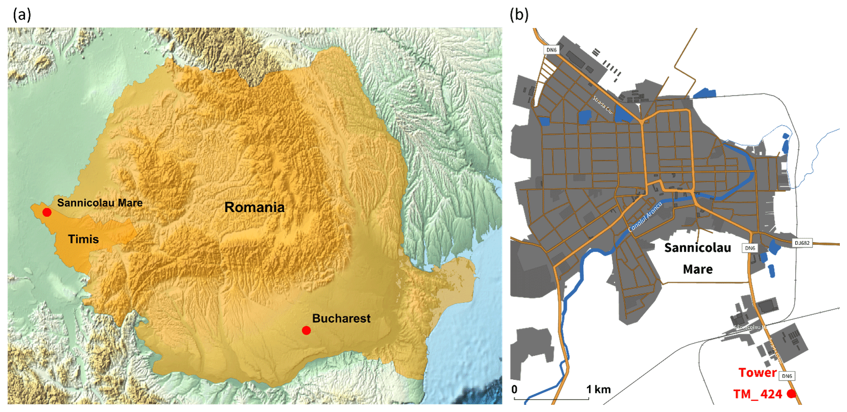
Figure 1 (a) Location of telecommunication tower TM_424, situated 1 km south of Sânnicolau Mare in Timiș County, Romania. (b) Expanded view of the town of Sânnicolau Mare with telecommunication tower TM_424 represented by the red dot on the map. Maps generated using Mathematica (Wolfram Research, Inc., version 13.3, 2023, https://www.wolfram.com/mathematica (last access: 27 November 2023).

Figure 2 shows the dimension of the tower. Among the various networks for the monitoring systems, the tower is equipped with a Gill WindObserver 70 ultrasonic anemometer at the top (Fig. 2). The anemometer has a data acquisition rate of 4 Hz and can measure the wind speed up to 70 m s⁻¹. In addition to the anemometer sensor, the tower is equipped with a temperature sensor installed near the location of the anemometer. The working temperature range for this sensor is between −55 and 70 °C.

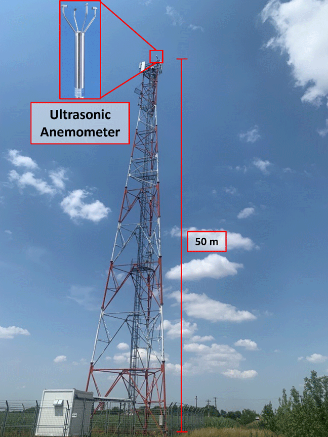
Figure 2 Telecommunication tower TM_424 and sensor position at the top of the tower. On the horizon, approximately 1 km from the tower, lies the small city of Sânnicolau Mare.

3 The Sânnicolau Mare (Romania) downburst event of 25 June 2021

In this section, a brief overview of the meteorological aspects pertaining to the downburst event in Sânnicolau Mare on 25 June 2021 is provided. In the late afternoon of 25 June 2021, a severe downburst event affected the far-western region of Romania. The downburst event took place in Timiș County (Fig. 1a) between 18:00 and 19:00 UTC and struck the little town of Sânnicolau Mare (Fig. 1b). At 17:30 UTC, a strong mesoscale convective system moving toward the east was approaching the town of Sânnicolau Mare. Figure 3a, acquired from EUMETSAT, captures an image of a deep convective cell at 18:30 UTC. This weather phenomenon exhibits cloud tops ascending over 12 km above mean sea level, signifying the mature stage of the convection cycle. This mature storm cell was observed to have directly impacted the town under study. Figure 3b presents composite radar reflectivity data, indicating that this meteorological phenomenon can be classified as a mesoscale convective system known as a bow echo. Radar reflectivity values at or above 60 dBZ, as seen in this event, are typically indicative of severe weather conditions. Such conditions are often associated with the production of hailstones, with an average diameter of approximately 2.5 cm.

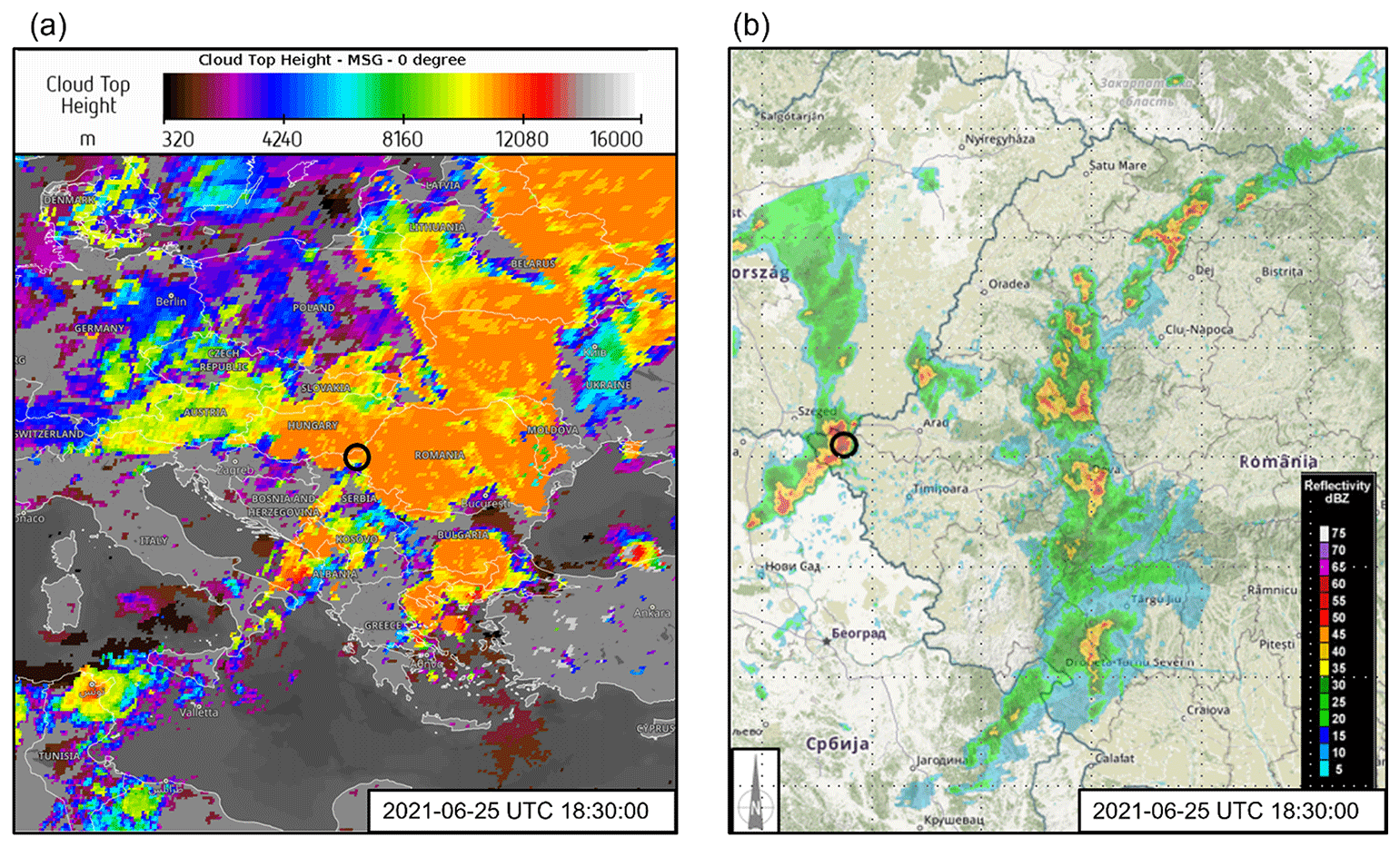
Figure 3 (a) Distribution of cloud top heights derived from Meteosat Second Generation (MSG) valid for 25 June 2021 at 18:30 UTC. Data and map obtained from © EUMETSAT 2022 (https://view.eumetsat.int, last access: 27 November 2023). (b) Composite radar reflectivity (dBZ) for 25 June 2021 at 18:30 UTC. The geographical locations of Sânnicolau Mare and the apex of the bow echo are indicated by the black circle. Data and map obtained from © 2018 Administraţia Naţională de Meteorologie (https://www.meteoromania.ro, last access: 27 November 2023).

The existence of a robust convective motion, indicative of the typical kinematic structure of a bow echo, is distinctly portrayed through the distribution of intensive lightning activity, as displayed in Fig. 4a. As the figure illustrates, an approximate total of 10 455 lightning strikes were recorded by the Blitzortung.org network across eastern Europe between 16:30 and 18:30 UTC. A significant concentration of these strikes correlates with the bow echo structure near the western edge of Timiș County, Romania. The color gradient in Fig. 4a, ranging between red, orange, yellow, and white, serves as a temporal marker, with white indicating the most recent strikes and red denoting older ones. This color coding effectively illustrates the temporal and spatial evolution of the lightning activity during the severe weather event, providing insight into the progression of the storm system. Bow echoes are a prevalent form of severe convective organization. These mesoscale convective systems can generate straight-line surface winds that lead to extensive damage associated with downbursts. On occasion, they may also give rise to tornadoes. Interestingly, the observed bow echo seems to display a stratiform parallel structure, a rarer variety of squall lines (Parker and Johnson, 2004; Markowski and Richardson, 2010).

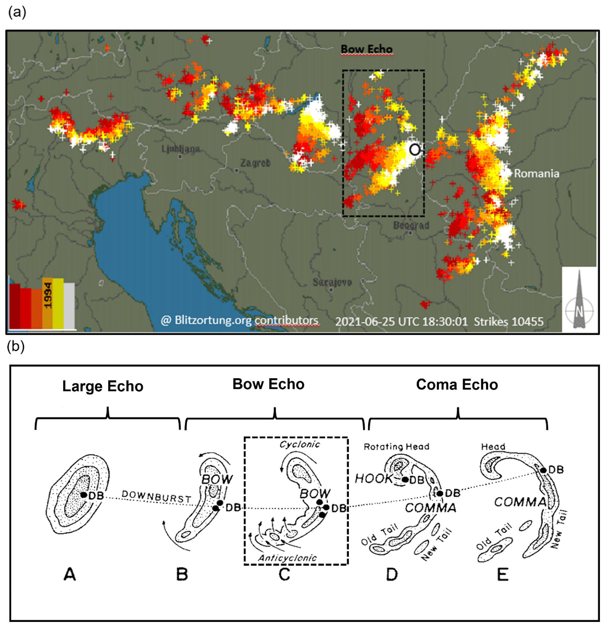
Figure 4 (a) Lightning strikes recorded between 16:30 and 18:30 UTC on 25 June 2021, sourced from the Blitzortung.org network archive for lightning and thunderstorms (https://www.blitzortung.org, last access: 6 October 2023). The black circle marks the geographic location of Sânnicolau Mare, situated near the apex of the observed bow echo. (b) Typical radar echo morphology commonly observed in bow echoes, characterized by the generation of strong downbursts at the bow apex, denoted as DB. Adapted from Fujita (1978).

Figure 4b illustrates the characteristic kinematic structure of a bow echo as outlined by Fujita (1978). Typically, the system originates as a singular, prominent convective cell, either isolated or embedded within a broader squall line system (Phase A). As the surface winds strengthen, the parent cell undergoes transformation, evolving into a line segment of cells with a bow-shaped configuration (Phase B). At maximum intensity, the bow's center might develop a spearhead echo (Phase C), characterized by the occurrence of the most severe downburst winds at the apex of the spearhead. During the decay phase, the wind system frequently evolves into a comma-shaped echo (Phase E) (Weisman, 2001). Comparing Figs. 3b, 4a, and 4b shows that the bow echo positioned above Sânnicolau Mare at 18:30 UTC is in its most intense stage (Phase C), as evidenced by the formation of the characteristic spearhead echo shape. The intense downburst event generated at the apex of the bow echo was recorded by the anemometer and temperature sensor situated 50 m above the ground on TM_424. The time histories of the moving-average wind speed and direction (averaged over 30 s) (Solari et al., 2015; Burlando et al., 2017) for the recorded 1 h duration of the downburst event are given in Fig. 5a and b, respectively. At approximately 18:30 UTC the anemometer recorded an instantaneous maximum velocity (sampled at 4 Hz) of $\widehat{V}=$ 40.8 m s⁻¹, while the maximum moving-average wind velocity was V_max=35.8 m s⁻¹. This notable high velocity clearly shows evidence of the occurrence of an intense downburst. The time interval spanning from 18:20 to 18:45 UTC represents the primary indicator of the downburst's occurrence in proximity to the telecommunication tower. This period is characterized by a sudden surge in wind speed, commonly referred to as the intensification stage, followed by a subsequent decrease in velocity after 18:30 UTC. Throughout the initial phase of intensification, the wind direction exhibited a clockwise rotation, ranging from 235° and extending to approximately 360°. Additionally, Fig. 5a also includes 1 h time series of the recorded temperature data. The temperature sensor is positioned at the same location of the anemometer. Before the passage of the downburst, the environmental temperature was on average 27 °C, while at approximately 18:20 UTC the temperature dropped very sharply, reaching the minimum value of 14.5 °C at approximately 18:30 UTC. After the sharp drop the temperature started to rise and eventually returned to its pre-storm level (not shown).

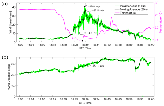
Figure 5 Telecommunication tower monitoring network measurements from 18:00 to 19:00 UTC on 25 June 2021: (a) time history of the instantaneous wind speed (green), moving-average mean wind speed (black), and temperature record (magenta) and (b) instantaneous (green) and moving-average mean wind direction (black).

The downburst in Sânnicolau Mare was also marked by a substantial hail occurrence. The interaction between the high-velocity winds and hail, potentially influencing the trajectory and impact of the hailstones, contributed to extensive damage, especially to the facades of numerous buildings. To comprehensively assess this damage, a collaborative survey was conducted by the University of Genoa (Italy) and the Technical University of Civil Engineering of Bucharest (UTCB) (Calotescu et al., 2022, 2024). The survey identified the affected buildings and produced a comprehensive map illustrating the hail damage. Figure 6 shows a schematic representation of the distribution of hail damage per area (600 × 600 m²) and the location of the buildings that suffer hail damage in the town of Sânnicolau Mare. Correlating specific damage like hail impacts with near-surface wind velocities involves inherent uncertainties, which are extensively explored in the study by Calotescu et al. (2024).

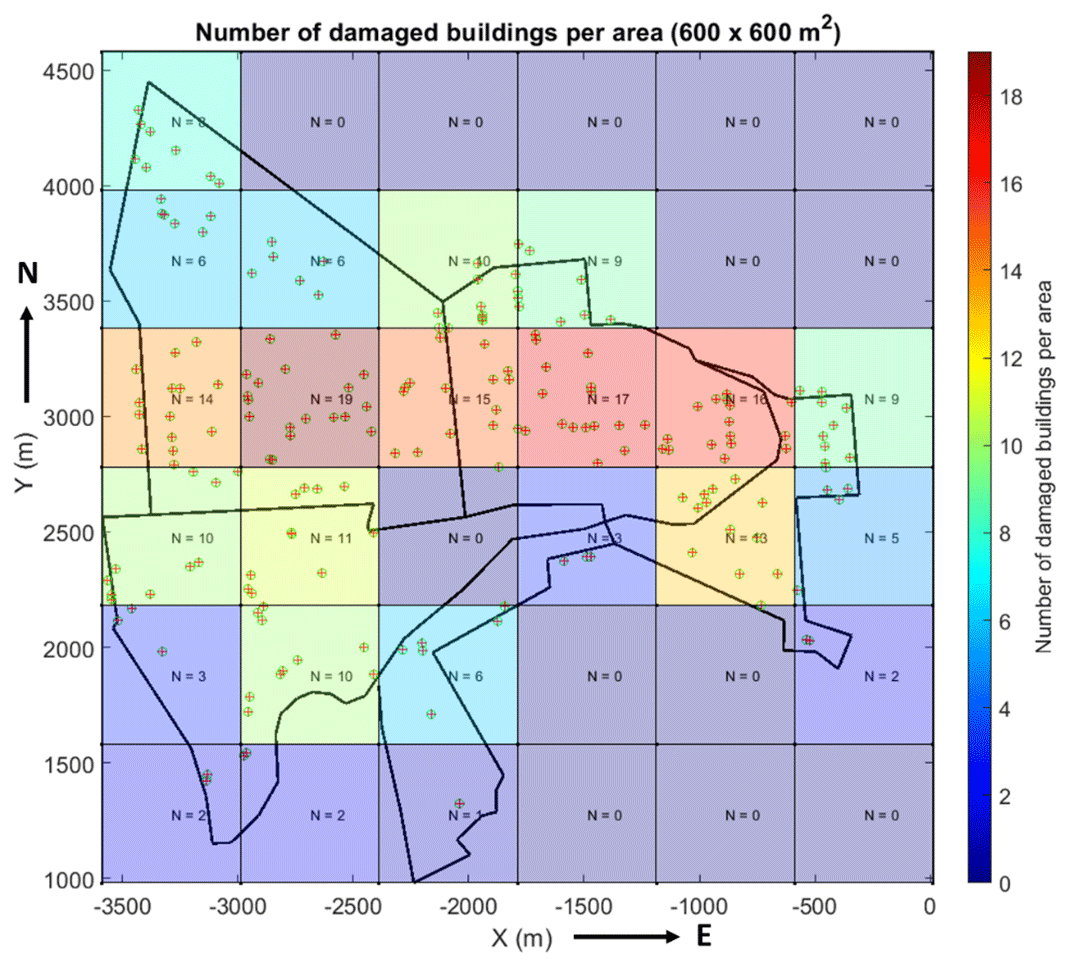
Figure 6 Spatial distribution of damaged buildings and locations of hail-damaged structures within the 600 × 600 m² area in the town of Sânnicolau Mare during the downburst event on 25 June 2021. The city boundaries of Sânnicolau Mare are delimited by the black line.

4 Downburst reconstruction

This section focuses on the modeling, optimization, and reconstruction of the Sânnicolau Mare downburst event. Section 4.1 delves into the modeling and optimization approach used for downburst reconstruction. Section 4.2 introduces metaheuristic optimization and its application in the reconstruction of the specific downburst event under study. Finally, Sect. 4.3 outlines the multivariate data analysis employed to examine the solutions generated by the optimization algorithm.

4.1 Modeling and optimization approach for downburst reconstruction

In this study, the authors utilize the computational model developed in a previous work by Xhelaj et al. (2020) for the reconstruction and simulation of the Sânnicolau Mare downburst event discussed in Sect. 3. The Xhelaj et al. (2020) model can simulate the spatiotemporal evolution of the bi-dimensional moving-average (30 s window) wind speed and direction experienced during a typical downburst event at a specified height z above ground level. In general, the wind system simulated by the analytical model represents the outflow structure of a translating downburst, typically occurring in diverse meteorological conditions such as single-cell thunderstorms, multicell thunderstorms, squall lines, and bow echoes. For the specific case of the Sânnicolau Mare downburst, the analytical model operates under the hypothesis that the downburst occurs near the tip of the bow echo during its mature stage (Phase C, Fig. 4b), in line with the studies of Fujita (1978) and Weisman (2001). It is worth noting that the model does not encompass the broader, complex mesoscale circulations, commonly associated with high winds in bow echoes. This represents a focused approach, considering the downburst evolution within a specific context, rather than attempting to model the entire spectrum of atmospheric phenomena related to bow echoes.

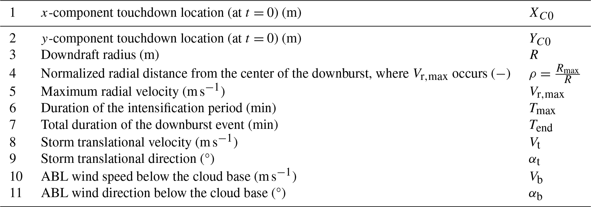
The analytical model comprises 11 variables that describe the kinematic structure of the downburst wind. Table 1 presents a short description of the 11 variables upon which the model relies. As a result, the model allows for the reconstruction of the time-evolving moving-average wind speed and direction generated by the simulated downburst at every point within the simulation domain. The model simulates the downburst wind velocity field by combining three components, the stationary radial velocity from a jet impacting a flat surface, the downdraft's translation velocity (i.e., storm motion), and the low-level ABL wind velocity. The virtual anemometer, situated at the center of the simulation domain, measures the simulated wind speed and direction generated by the model. By employing anemometric wind speed and direction data collected during the Sânnicolau Mare downburst event, an optimization procedure can be formulated to minimize the relative error (objective function F), which quantifies the discrepancy between the observed time series of the moving-average wind speed and direction and the corresponding simulations generated by the model. Since the Sânnicolau Mare downburst event was recorded by an anemometer positioned at a height of 50 m a.g.l., the analytical model will reconstruct the wind speed and direction at the corresponding height.

Table 1 Variables of the Xhelaj et al. (2020) analytical model.

The reconstruction procedure gives rise to a mathematical optimization problem characterized by being single-objective, nonlinear, and bound-constrained, as discussed in Xhelaj and Burlando (2022). To tackle this optimization problem, the analytical model is integrated with a global metaheuristic optimization algorithm. Specifically, the teaching–learning-based optimization (TLBO) algorithm proposed by Rao et al. (2011) is employed. The details pertaining to the integration of the analytical model with the optimization algorithm, as well as the estimation of the kinematic and geometric variables associated with the downburst event, are explained in detail in Xhelaj and Burlando (2022). The MATLAB code for performing this procedure is available in the repository by Xhelaj (2024). The TLBO algorithm is an iterative, stochastic, and population-based algorithm comprising two distinct phases: the teacher phase and the learner phase. In the teacher phase, the best solution in the population (the teacher) shares its knowledge (objective function) with the other solutions (the students) to enhance their performance. In the learner phase, the students interact with each other to further improve their performance. TLBO requires only two user-specified parameters: the maximum number of iterations T and the population size N_p. When incorporating the objective function into a stochastic metaheuristic optimization algorithm, running the algorithm independently multiple times is crucial to reach the optimal solution. This iterative approach allows for a deeper exploration of the variable space, reducing the risk of getting trapped in local optima. However, it is important to note that in the context of metaheuristic optimization, there is no guarantee of attaining a globally optimal solution. As a result, the procedure can yield a range of solutions ordered based on the values assumed by the objective function, with some being better than others. In this study, the TLBO algorithm is executed 1024 times independently, with each run producing an optimal solution. Consequently, 1024 solutions are obtained. The reconstruction of the downburst event can be accomplished by selecting the solution with the lowest objective-function value, as it is considered the best representation of the event based on the optimization process. This study aims to analyze and clarify the nature of all the solutions generated by means of the TLBO algorithm for the downburst outflow reconstruction. This choice was made for two reasons.

• The first reason is to determine the best possible solution among the 1024 runs, where the best solution is the one that minimizes the objective function F and allows for reconstructing the Sânnicolau Mare downburst event.

• The second reason, which is the primary objective of this study, is to analyze these 1024 solutions using multivariate data analysis (MDA). The method used in MDA is the agglomerative hierarchical K-means clustering (AHK-MC) and principal component analysis (PCA).

The objective is to investigate the distinct characteristics of the different solutions provided by the TLBO algorithm, enabling an understanding of their divergence from the optimal solution. If alternative solutions do exist, it signifies that the algorithm's solution is not unique. This highlights the challenge in accurately reconstructing the downburst wind field form just one anemometric time series, underlining the problem's inherent complexity and underdetermined nature. As such, a more comprehensive definition of the objective function is necessary to accurately discern between the optimal solution and its alternatives.

4.2 Metaheuristic optimization and reconstruction of the Sânnicolau Mare downburst

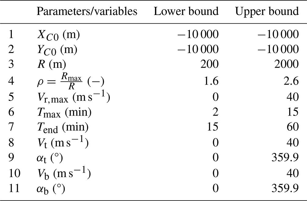
In metaheuristic optimization, a commonly used guideline suggests setting the population size N_p as 10 times the number of variables to estimate D (Storn, 1996). In this study, where D corresponds to 11 variables, a population size of N_p=110 has been chosen. Additionally, considering the reported fast convergence rate of the TLBO algorithm (as mentioned in Xhelaj and Burlando, 2022), the maximum number of iterations T for this study has been set to T=100. Table 2 displays the lower and upper bounds of the optimization problem pertaining to the reconstruction of the Sânnicolau Mare downburst. These parameter values have been determined based on a comprehensive literature review, available in Xhelaj and Burlando (2022).

Table 2 Lower and upper bound of the decision variable parameters for the reconstruction of the Sânnicolau Mare downburst. Table form Xhelaj and Burlando (2022).

The spatial domain of the downburst simulation covers an area of 20 × 20 km², while the grid resolution in both the X and Y directions is set at 50 m. This approach employs a comprehensive simulation approach, primarily using anemometric data, due to its common availability. The methodology entails numerous simulations to extract a downburst's kinematic and geometric parameters. However, when additional data like radar or lidar are available, this information can be used to bound some variables and restrict the model variables domain (Table 2) to enhance model accuracy. Figure 7 illustrates the “performance chart” depicting the convergence pattern of the objective functions during the reconstruction of the Sânnicolau Mare downburst using the TLBO algorithm. The performance chart in Fig. 7 illustrates the convergence pattern of the objective functions as an iterative progress. It shows the upper and lower envelopes that encapsulate all 1024 independent runs. The region within the envelopes represents the objective-function values' trend for all runs. At the end of the 100 iterations, the lower envelope represents to the best objective-function value obtained, while the upper envelope corresponds to the worst objective-function value obtained by the TLBO algorithm. The performance chart in Fig. 7 includes additional visual representations: a dashed line representing the mean convergence curve and dotted lines representing curves of the mean plus/minus 1 standard deviation. These curves provide insights into the average behavior and deviation of the objective-function values across the 1024 runs. The performance chart demonstrates that after approximately 70 iterations, the TLBO algorithm ceases to find significantly better or worse solutions. This is evidenced by the convergence of both the upper and lower envelope curves. Concurrently, the mean curve appears to plateau, although it exhibits a slight yet continuous improvement beyond the 70th iteration. This suggests that the algorithm is still optimizing, albeit at a reduced rate. The increasing spread between curves of the mean plus/minus 1 standard deviation as the iterative progress indicates a complex solution landscape. This complexity is manifested in the algorithm's convergence to various local minima, maintaining steady average performance while increasing the variability of solutions. In this study's context, such an expanding spread represents a deeper and more intricate exploration of the solution space, a desirable characteristic to ensure a comprehensive search across the objective-function domain. At the conclusion of 100 iterations, the best and worst objective-function values correspond to F_min= 0.730 and F_max = 1.062, respectively. The mean and standard deviation of the objective-function values are determined as m_F= 0.893 and s_F= 0.080, respectively.

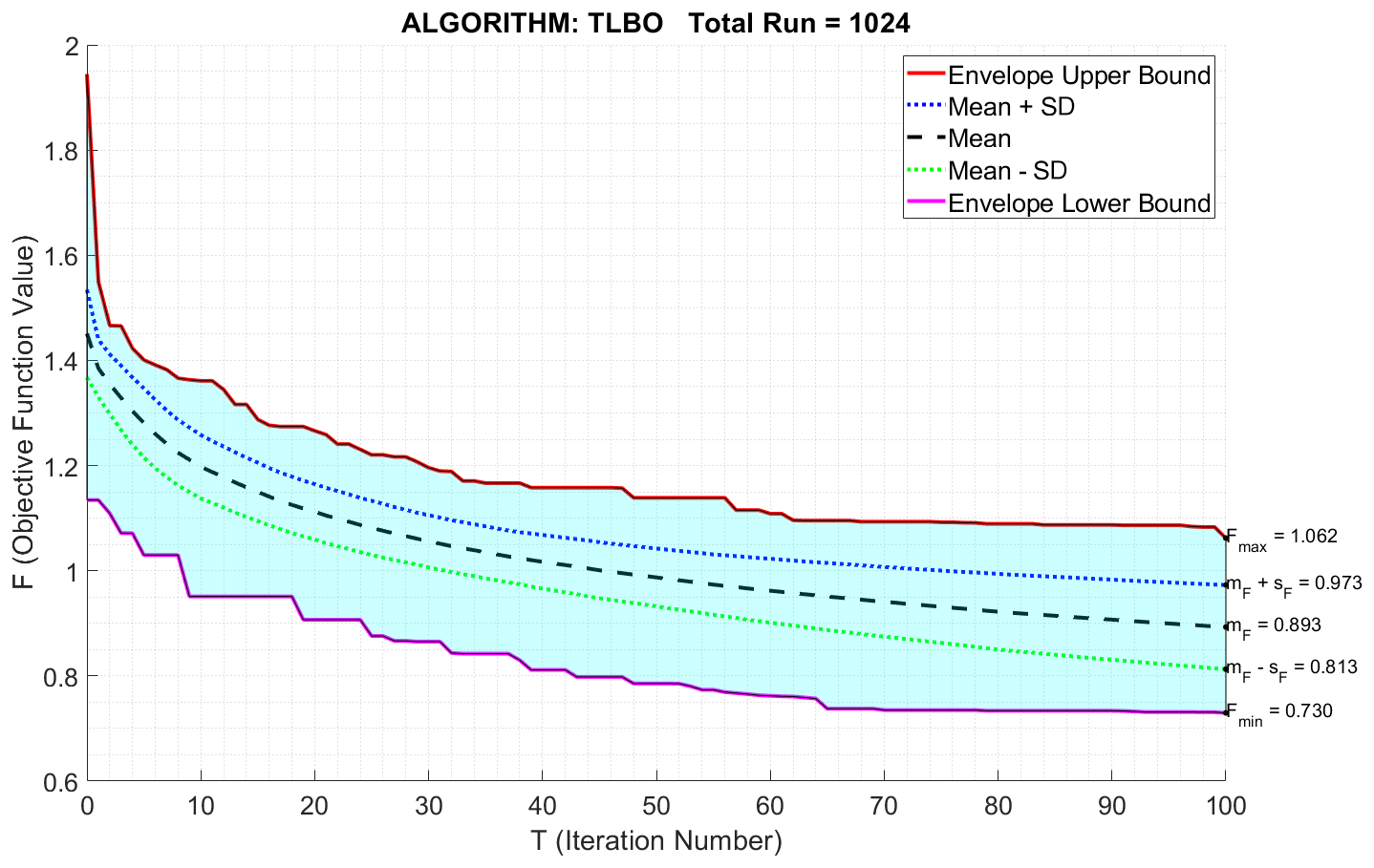
Figure 7 Performance chart for the reconstruction/simulation of the Sânnicolau Mare downburst using the TLBO algorithm.

4.3 Multivariate data analysis of solutions for the Sânnicolau Mare downburst reconstruction

The optimization algorithm provides output as a data table, where each row of the table is a solution of the optimization problem. Therefore, the data table is composed of 1024 rows (solutions). The table has 12 columns, where 11 columns represent the 11 variables/parameters of the analytical model, while the last column contains the values assumed by the objective function F of each solution (i.e., each row). Although the objective function F is not a variable of the analytical model, it is treated in Sect. 5 as a variable from the point of view of the multivariate data analysis. The solutions are sorted in descending order based on their objective function F. This means that the best overall solution among the 1024 lies in the last row of the data table. The analysis of the data table indicates that most variables exhibit multimodal histograms, with two or more peaks. However, only the variables V_b and α_b are characterized by a unimodal histogram. Since the aim of this document is to conduct a multivariate data analysis (MDA), the variables of the data table are split into primary and secondary variables. Primary variables participate in the analysis of multivariate data (i.e., AHK-MC and PCA), as opposed to secondary variables, which have no role in the calculation. However, secondary variables can indeed assist in the interpretation of the data table. In the present study, V_b, α_b, and α_t are considered secondary variables. This choice is primarily driven by the observation that V_b and α_b exhibit unimodal histograms, suggesting that they may not significantly contribute to distinguishing different cluster solutions. However, the choice of α_t as a secondary variable is purely practical, since it makes it possible to carry out a multivariate statistical analysis, avoiding the problem of circular statistics and, hence, simplifying the calculation and the interpretations of the results.

Let us define the data table that contains only primary variables by a matrix 𝕏. Each row i of the matrix represents a solution vector X_i, encompassing the values associated with the nine primary variables. Therefore the solution vector can be expressed as ${\mathit{X}}_i={\left(X_{C{\mathrm{0}}_i},Y_{C{\mathrm{0}}_i},R_i,{\mathit{\rho }}_i,V_{\mathrm{r},{\max }_i},T_{{\max }_i},T_{f_i},V_{t_i},F_i\right)}^T$ with i ranging from 1 to I, where I represents the total number of solutions, in this case I= 1024. Since the solution vector X_i contains K =9 primary variables, the resulting data matrix 𝕏 is an I×K matrix with 1024 rows and 9 columns. For the sake of simplicity, in order to shorten the notation, let X_ik be the value of the kth primary variable in the ith solution. Henceforth, the term “variable” will refer to primary variables, unless explicitly specified. Consequently, the dataset within the matrix 𝕏 can be regarded either as a collection of rows representing solutions to the optimization problem or as a collection of columns representing variables of the analytical model. The focus of MDA is to apply statistical clustering to identify similar analytical solutions. Since a generic solution 𝕏 is a set of K = 9 numerical values, 𝕏 evolves within a space R^K (a space with nine dimensions), called “the solution space”. By defining the usual Euclidean metric in the solution space (i.e., the l₂ norm ∥⋅∥₂), the squared distance between two solutions X_i and X_l can be expressed by the Euclidean distance d_il.

$$\begin{array}{}\text{(1)}& d_{il}^{\mathrm{2}}=d^{\mathrm{2}}\left({\mathit{X}}_i,{\mathit{X}}_l\right)={∥{\mathit{X}}_i-{\mathit{X}}_l∥}_{\mathrm{2}}^{\mathrm{2}}=\sum _{k=\mathrm{1}}^K{\left(X_{ik}-X_{lk}\right)}^{\mathrm{2}}.\end{array}$$

The distance d possesses the following metric properties:

$$\begin{array}{}\text{(2)}& \left\{\begin{array}{ll}d({\widehat{\mathit{X}}}_i,{\widehat{\mathit{X}}}_l)& =\mathrm{0}\iff i=l,\\ d({\widehat{\mathit{X}}}_i,{\widehat{\mathit{X}}}_l)& =d({\widehat{\mathit{X}}}_l,{\widehat{\mathit{X}}}_i)\left(\mathrm{symmetry}\right),\\ d({\widehat{\mathit{X}}}_i,{\widehat{\mathit{X}}}_l)& \le d({\widehat{\mathit{X}}}_i,{\widehat{\mathit{X}}}_j)+d({\widehat{\mathit{X}}}_j,{\widehat{\mathit{X}}}_l)\left(\mathrm{tirangle}\mathrm{inequlity}\right).\end{array}\right.\end{array}$$

Variables in the data matrix 𝕏 are standardized to account for different units and scales. This common practice in statistical modeling neutralizes scale effects, allowing for meaningful comparisons across variables. Therefore, the variables are standardized according to the following equation:

$$\begin{array}{}\text{(3)}& \begin{array}{rl}{\widehat{X}}_{ik}& ={\displaystyle \frac{X_{ik}-{\stackrel{\mathrm{‾}}{X}}_k}{S_k}},\forall i=\mathrm{1},\mathrm{\dots },I=\mathrm{1024}\\ & \mathrm{and}\forall k=\mathrm{1},\mathrm{\dots }K=\mathrm{9},\end{array}\end{array}$$

where ${\stackrel{\mathrm{‾}}{X}}_k$ denotes the sample mean of the kth variable calculated over all I solutions, ${\stackrel{\mathrm{‾}}{X}}_k=\frac{\mathrm{1}}{I}{\sum }_{I=\mathrm{1}}^I{X}_{ik}$, and S_k is the sample standard deviation of kth variable, $S_k=\sqrt{\frac{\mathrm{1}}{\left(I-\mathrm{1}\right)}{\sum }_{i=\mathrm{1}}^I{\left(X_{ik}-{\stackrel{\mathrm{‾}}{X}}_k\right)}^{\mathrm{2}}}$.

Finally, the normalized data matrix $\widehat{\mathbb{X}}$ containing the set of vectors ${\widehat{\mathit{X}}}_i$, $i=\mathrm{1},\mathrm{\dots },I$ has been used in the MDA for the identification of different typologies of solutions provided by the TLBO algorithm for the simulation/reconstruction of the Sânnicolau Mare downburst. Figure 8 showcases a summary statistic in the form of a box plot, illustrating the distribution of the standardized variables. Variables such ${\widehat{\mathit{R}}}_{\max }$ and ${\widehat{\mathit{T}}}_{\max }$ have a large number of outliers, indicating extreme values within the dataset. Therefore, even in the context of standardized data, outliers can still be informative and may hold important information for distinguishing distinct solution clusters. All the multivariate statistical analyses in this work were performed using the online version of the software FactoMineR (Lê et al., 2008).

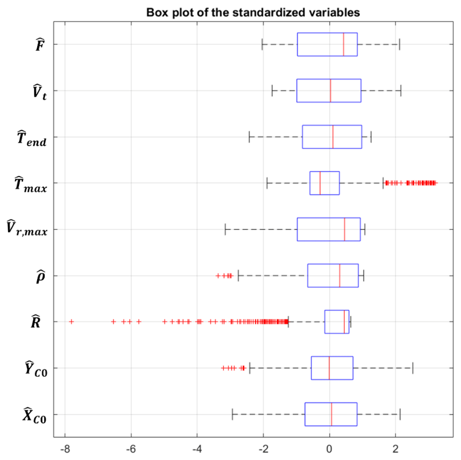
Figure 8 Box plot of the distributions of the standardized variables. Outliers in the data are plotted individually using the red marker symbol +.

5 Results

In the following section the results of multivariate data analysis (MDA) including cluster analysis and principal component analysis applied to the data matrix $\widehat{\mathbb{X}}$ are presented. After the clusters have been established a comprehensive description of each of them is provided. This involves examining the variables that contribute to each cluster's composition as well as identifying specific representative solutions within each cluster. Such an analysis allows for a deeper understanding of the cluster characteristics and facilitates the interpretation of meaningful patterns and insights within the data. The text in Sect. 5.1 to 5.3 provides an in-depth analysis of the data matrix $\widehat{\mathbb{X}}$ from the variable's perspective, employing agglomerative hierarchical K-means clustering and principal component analysis. In Sect. 5.4 the clusters are analyzed from the point of view of the specific solutions which are the most representative of the clusters. Finally, these representative solutions are compared with the best overall solution found by the TLBO algorithm. The comparisons of the representative solution for each cluster and the best overall solution with the full-scale data are therefore enriched considering the data from the damage survey that was carried out after the Sânnicolau Mare downburst event.

5.1 Identification of the most meaningful clusters

In order to identify the appropriate number of clusters for grouping the solutions, agglomerative hierarchical clustering (AHC) is firstly employed (Hartigan, 1975; Kaufman and Rousseuw, 1990). In AHC, each individual solution is initially treated as an independent cluster (leaf). Through a series of iterative steps, the most similar clusters are progressively merged, forming a hierarchical tree structure known as a dendrogram. This merging process continues until all the individual clusters are combined into a single cluster (root).

Subsequently, the hierarchical tree is analyzed, and a suitable level is chosen to cut the tree, leading to distinct and meaningful clusters. The number of clusters obtained from AHC forms a partition of the dataset. To refine and optimize this partition, a partitioning clustering algorithm called K-means clustering (MacQueen, 1967; Hartigan and Wong, 1979) is subsequently applied. Partitioning algorithms, like K-means clustering, subdivides the datasets into distinct clusters, ensuring that solutions within each cluster are similar to one another, while exhibiting noticeable differences between clusters. Hence the two steps clustering procedure is called agglomerative hierarchical K-means clustering (AHK-MC) and is employed to analyze the standardized data matrix $\widehat{\mathbb{X}}$. By combining the strengths of both AHC and K-means clustering, AHK-MC aims to provide a comprehensive and improved clustering algorithm of the data, enabling a more accurate identification of distinct solution groups.

The hierarchical tree in Fig. 9 (i.e., dendrogram) is constructed following Ward's method (Ward, 1963). Since the total solutions of the optimization problem are I = 1024, the dendrogram is very dense at the bottom level (i.e., at the leaf level, where each solution is considered a cluster by itself). The hierarchical tree is composed therefore by $I-\mathrm{1}=\mathrm{1023}$ nodes, with the points being where two clusters (solutions or set of solutions) are merged. The level (height) of each node in the tree is described by the within-cluster variance. The level of a node in the agglomeration process, when examined from top to bottom, indicates the reduction in within-cluster variance achieved by merging two connected clusters. This reduction in variance can be visualized using a bar graph, as depicted in Fig. 10.

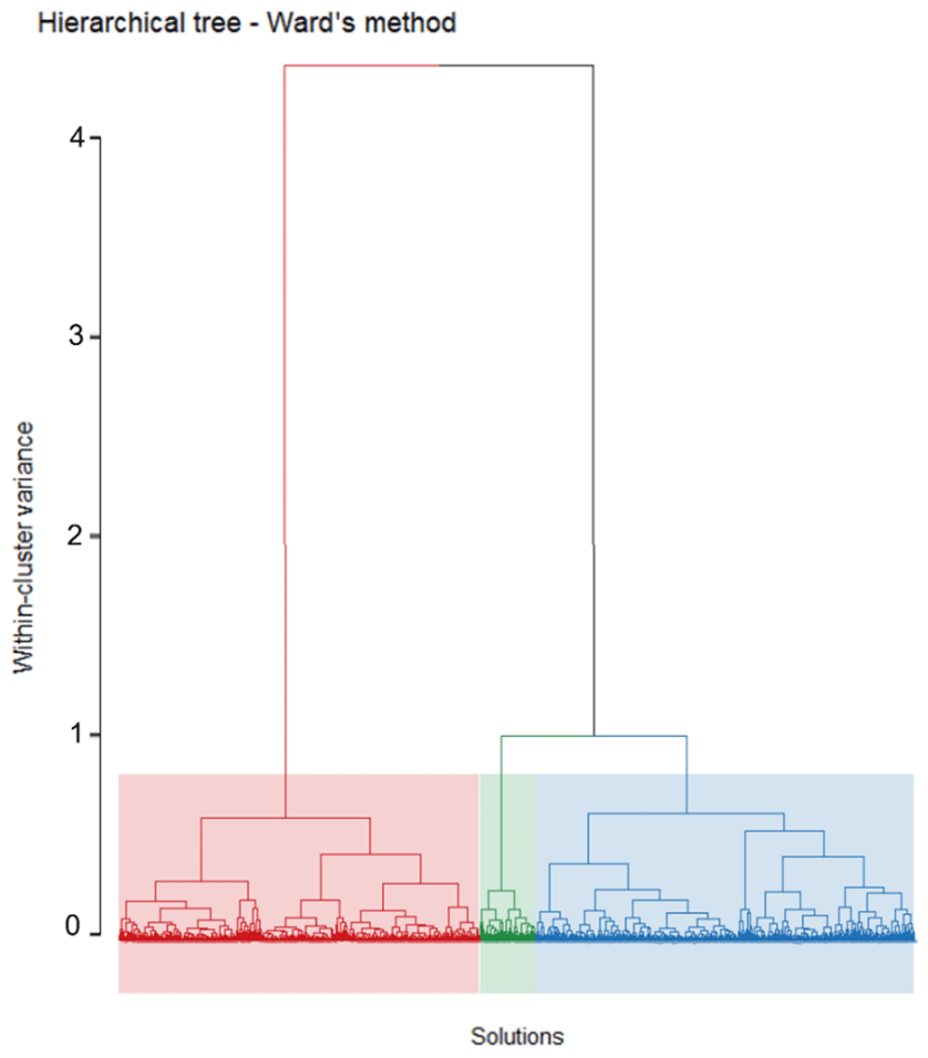
Figure 9 Hierarchical tree (dendrogram) created with Ward's method, categorizing the optimization problem solutions for the Sânnicolau Mare downburst into three clusters, each marked by a distinct color: red for cluster 1, green for cluster 2, and blue for cluster 3.

From Fig. 10 it is possible to establish the level where to cut the dendrogram and consequently to establish the number of clusters for partitioning the dataset. The choice of the number of clusters is important because partitioning with too few clusters risks leaving groups which are not at all homogeneous. On the other hand, partitioning with too many clusters risks creating classes that are not very different from each other. Being ${\sum }_{s=\mathrm{1}}^{I-\mathrm{1}}{\mathrm{\Delta }}_{\mathrm{s}}=K=$ 9 (the total variance contained in the standardized data), the separation into two groups is able to describe $\mathrm{\Delta }\left(\mathrm{1},\mathrm{2}\right)/K=\mathrm{4.314}/\mathrm{9}=$ 0.4793 (47.93 %) of the total variance. Considering the partitioning into three groups, the explained variance by the three clusters is equal to $\left[\mathrm{\Delta }\left(\mathrm{1},\mathrm{2}\right)+\mathrm{\Delta }\left(\mathrm{2},\mathrm{3}\right)\right]/K=\left[\mathrm{4.314}+\mathrm{1.044}\right]/\mathrm{9}=\mathrm{0.5954}$ (59.54 %) of the total variance, while for four clusters the “explained variance” is equal to $\left[\mathrm{\Delta }\left(\mathrm{1},\mathrm{2}\right)+\mathrm{\Delta }\left(\mathrm{2},\mathrm{3}\right)+\mathrm{\Delta }\left(\mathrm{3},\mathrm{4}\right)\right]/K=\left[\mathrm{4.314}+\mathrm{1.044}+\mathrm{0.406}\right]/\mathrm{9}=\mathrm{0.6404}$ (64.05 %) of the total variance.

Therefore, considering more than three clusters (refer to Fig. 10) is going to have a very little impact on the explained variance since very little information is gained and is no longer useful to group together any more classes. For this reason, the dendrogram in this work is partitioned into three clusters (refer to Fig. 9), and therefore they can explain approximately 60 % of the total variance present in the data.

The three-cluster solution's ability to explain about 60 % of the total variance is significant, especially considering the single-point (anemometric) measurement nature of the downburst data. This inherent limitation often leads to high variability, making the extraction of consistent patterns challenging. As noted in related studies, such as those by Bogensperger and Fabel (2021), benchmarks for acceptable levels of explained variance in clustering are not universally applicable but rather depend on the specific context and data characteristics. The present study's level of variance explanation, given the complexity and variability of the downburst captured from one location, is therefore robust. This is further supported by the observation in Fig. 10 that additional clusters contribute minimally to the total variance explained, suggesting that the primary structural patterns in the data are adequately captured with three clusters.

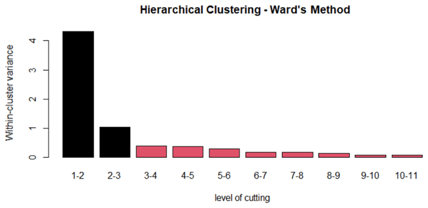
Figure 10 Bar graph of the relation between the number of merged clusters and the within-cluster variance.

5.2 Cluster interpretation via PCA and optimization with K-means clustering

The three clusters of solutions are analyzed using principal component analysis (PCA) to identify the key variables that drive the system's behavior. By extracting the principal components, which captures the most significant variation in the data, the complexity of the system can be reduced. In particular, the eigenvalues of the correlation matrix 𝕊= $\frac{\mathrm{1}}{\left(I-\mathrm{1}\right)}{\widehat{\mathbb{X}}}^T\widehat{\mathbb{X}}$ quantify the amount of variance accounted by each principal component (Kassambara, 2017). The eigenvalues show that the first components have larger values, indicating that they capture the most significant variation in the dataset. In contrast, the subsequent components have lower eigenvalues, representing a diminishing level of variation. Table 3 presents the eigenvalues, the percentage of variance explained by each component, and the cumulative percentage of variance.

Table 3 PCA results in terms of the eigenvalues, percentage of variance, and cumulative percentage of variance.

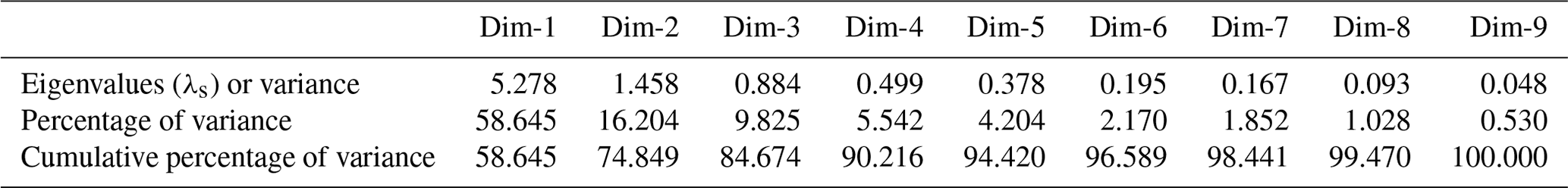
The first two principal components capture 74.85 % of the total variance in the dataset. These components define a plane that provides significant insights into the underlying patterns and structure of the data. Eigenvalues greater than 1 (Table 3) signify that the respective principal components explain more variance in the data compared to any single standardized variable. In contrast, eigenvalues less than 1, starting from the third principal component (Table 3), indicate that the associated principal components explain less variance than individual standardized variables, suggesting they have relatively less influence on the overall variability in the data. Therefore, it is probably not useful to interpret the next dimensions and better to focus on the first two principal dimensions for a more meaningful analysis. It is worth mentioning that the percentage of variance explained by the first principal component (58.65 %) is very close to the variance explained by the hierarchical tree when is partitioned into three clusters (59.54 %).

The three clusters, found using Ward's method only, are represented in terms of solutions in the principal component map (Fig. 11a). This figure shows how solutions are grouped together into three clusters when the overall cloud of solutions is projected into the first two principal components. Here, cluster 1 is not very well separated from cluster 3, which means that both clusters share similar solutions.

To enhance the distinctiveness of the cluster partitioning, the K-means algorithm is subsequently applied. This refinement step adjusts the initial partitioning obtained through Ward's method. The K-means algorithm optimizes cluster separation by iteratively recalculating the centroids for each cluster and reassigning solutions according to their proximity in Euclidean space. This procedure incrementally increases the ratio of between-cluster variance to the total variance, which results in the reduction in overlap and a clearer delineation of clusters. The process continues until the improvement in this variance ratio does not exceed a certain threshold, thus solidifying the partitioning. The iterative optimization by the K-means algorithm is what transforms the initial, less distinct cluster arrangement (Fig. 11a) into a final partitioning where clusters are well separated and more compact (Fig. 11b). This refined partitioning is not only more visually apparent but also statistically significant, and it is this final configuration that is retained for further analysis within the paper.

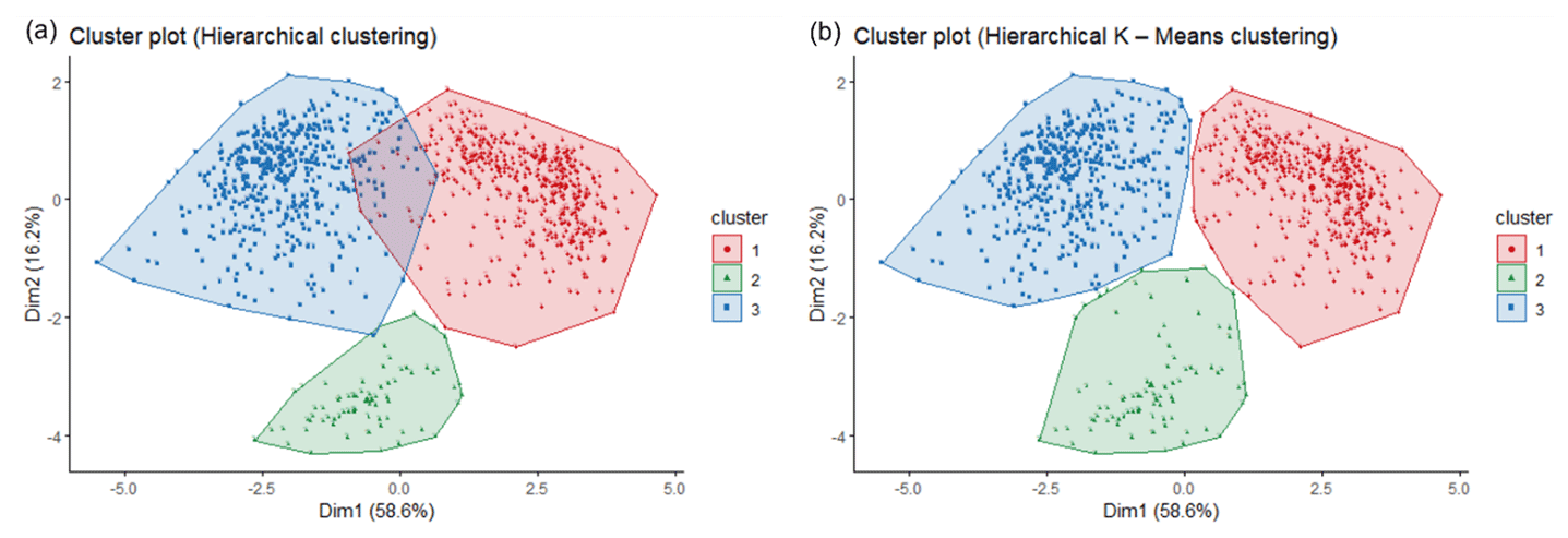
Figure 11 (a) Solution cluster partitioning on the principal component map using Ward's method only. (b) Solution cluster partitioning using the hierarchical K-means method.

5.3 Further considerations on the model's parameters

In Table 4, each standardized variable ${\widehat{\mathit{V}}}_k$ is presented as a vector, summarizing observations from the 1024 solutions. This forms the basis for the analysis focusing on the first two principal components, denoted as p₁ and p₂. The table displays the correlations $r_{\mathrm{s}}=r({\widehat{\mathit{V}}}_k,{\mathit{p}}_{\mathrm{s}}$) (where s= 1, 2) between the variables and these components (columns 1 and 4). Additionally, the table includes the quality of the representation qlt_s of each variable (columns 2 and 5) and the weight of each variable qtr_s in the construction of these components (columns 3 and 6). The quality of representation (${\mathrm{qlt}}_{\mathrm{s}}=r_{\mathrm{s}}^{\mathrm{2}}$) measures the extent to which a variable is accurately projected onto a principal component. The weight of a variable (${\mathrm{qtr}}_{\mathrm{s}}=\frac{r_{\mathrm{s}}^{\mathrm{2}}}{{\mathit{\lambda }}_{\mathrm{s}}}\cdot$ 100 %) quantifies the variable's relative contribution to the variance explained by the principal component, with λ_s being the eigenvalue corresponding to that component (Husson et al., 2017).

Table 4 Principal component analysis results for variables in terms of correlations (r), the quality of representation (qlt), and the contribution to the construction (qtr) relative to the first two principal components. ${\widehat{\mathit{V}}}_k$ represents the kth standardized variable; p₁ and p₁ denote the first and the second principal components, respectively.

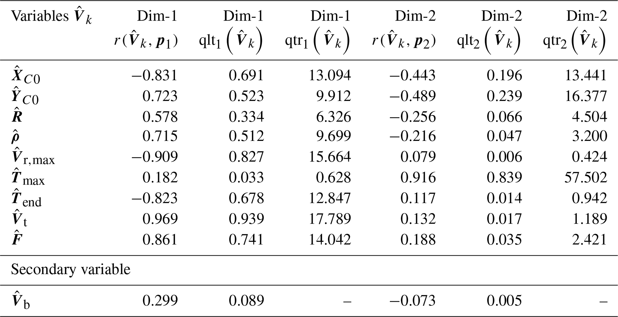
Table 4 also presents the secondary variable ${\widehat{\mathit{V}}}_{\mathrm{b}}$. The other two variables, ${\widehat{\mathit{\alpha }}}_{\mathrm{t}}$ and ${\widehat{\mathit{\alpha }}}_{\mathrm{b}}$, are not considered in the PCA due to their circular nature, which does not align well with the linear interpretation framework of principal component analysis. Despite ${\widehat{\mathit{V}}}_{\mathrm{b}}$ not being involved in the construction of the principal components, it is still possible to evaluate the correlation and the quality of the representation of this variable using the two principal components. To facilitate the interpretation of Table 4, a correlation circle plot (Abdi and Williams, 2010) can be used to visually represent the variables. This plot represents each variable as a point in a two-dimensional space, where the coordinates of each point correspond to the correlation coefficients between the variable and the two principal components (i.e., $r\left({\widehat{\mathit{V}}}_k,{\mathit{p}}_{\mathrm{1}}\right),r\left({\widehat{\mathit{V}}}_k,{\mathit{p}}_{\mathrm{2}}\right))$. Figure 12a illustrates the correlation circle plot.

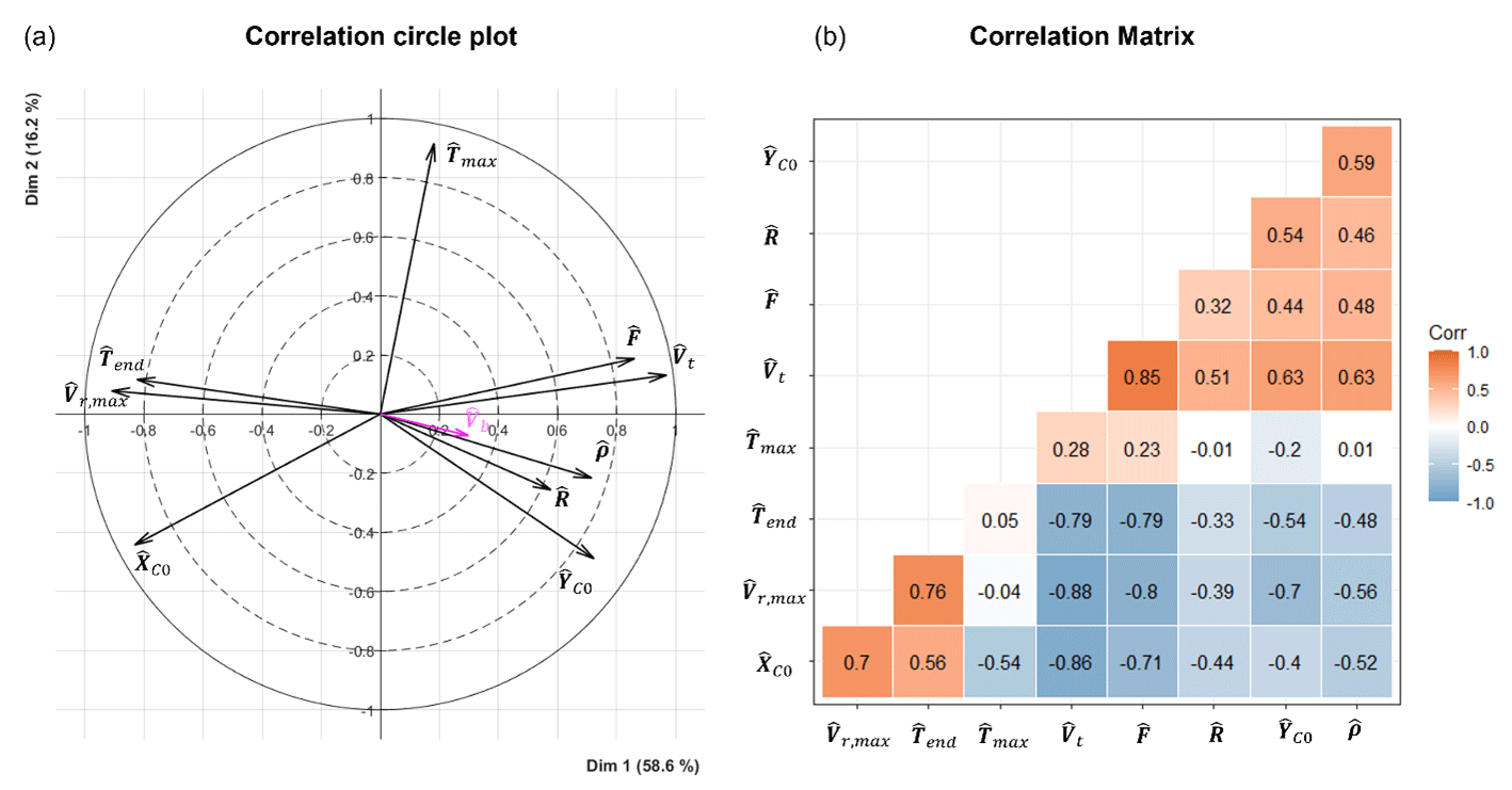
Figure 12 (a) Correlation circle plot. The variables in black are considered primary variables, whereas the variable in magenta is a secondary variable. (b) Correlation matrix plot.

The plot geometrically represents variable correlations: the angles between the variables indicate the level of correlations between variables, with acute angles suggesting positive correlation and obtuse angles indicating negative correlation. Each variable's total contribution across all principal components equals 1. Variables fully explained by the first two components will be located on the circle's circumference (radius of 1) in the correlation circle. Variables not well represented by these components will be near the center, indicating that only those near the circumference are significantly represented. Except for the variables ${\widehat{\mathit{V}}}_{\mathrm{b}}$ and $\widehat{\mathit{R}}$, which are not very well represented by the first two principal components, the remaining variables are very well represented since their tip is close to the circle with a radius of 1. The variables of {${\widehat{\mathit{V}}}_{\mathrm{t}}\widehat{\mathit{F}},{\widehat{\mathit{Y}}}_{C\mathrm{0}},\widehat{\mathit{\rho }}\mathit{\}}$ are positively correlated, increasing together, similarly to {${\widehat{\mathit{V}}}_{\mathrm{r},\max },{\widehat{\mathit{X}}}_{C\mathrm{0}},{\widehat{\mathit{T}}}_{\mathrm{end}}$}. The variable ${\widehat{\mathit{V}}}_{\mathrm{t}}$ is highly correlated with the first component (correlation of 0.97). Essentially ${\widehat{\mathit{V}}}_{\mathrm{t}}$ can be viewed as a representative summary of the first principal component axis. Figure 12a indicates that the variable ${\widehat{\mathit{V}}}_{\mathrm{t}}$ has a strong negative correlation with the variables of {${\widehat{\mathit{V}}}_{\mathrm{r},\max },{\widehat{\mathit{X}}}_{C\mathrm{0}},{\widehat{\mathit{T}}}_{\mathrm{end}}$}. This suggests that high storm motion values V_t correspond with lower maximum radial velocities V_r,max, with X_C0 being positive for a position closer to the station and negative for one farther away and a shorted downburst duration being represented as T_end.

Since ${\widehat{\mathit{V}}}_{\mathrm{t}}$ is positively correlated with the variables of {$\widehat{\mathit{F}},{\widehat{\mathit{Y}}}_{C\mathrm{0}},\widehat{\mathit{\rho }}$}, what is true for ${\widehat{\mathit{V}}}_{\mathrm{t}}$ with respect to the group of variables of {${\widehat{\mathit{V}}}_{\mathrm{r},\max },{\widehat{\mathit{X}}}_{C\mathrm{0}},{\widehat{\mathit{T}}}_{\mathrm{end}}$}, will also remain true for the variables of {$\widehat{\mathit{F}},{\widehat{\mathit{Y}}}_{C\mathrm{0}},\widehat{\mathit{\rho }}$}. Finally, from the correlation circle plot, it seems that the variable ${\widehat{\mathit{T}}}_{\max }$ is not very well “linearly” correlated with the variables of {${\widehat{\mathit{V}}}_{\mathrm{r},\max },{\widehat{\mathit{T}}}_{\mathrm{end}},\widehat{\mathit{\rho }}$} since it is nearly orthogonal with these variables. From a quantitative point of view the values of the correlation coefficients between all the pairs of variables are plotted in Fig. 12b. Table 4 lists each variable's contributions to the first and second principal components (columns 3 and 6, respectively). Figure 13a and b graph these contributions in percentages, showing which variables have the most impact on these two components.

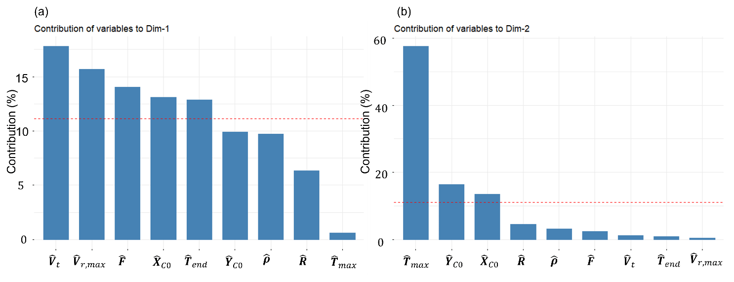
Figure 13 (a) Contribution of the variables in the reconstruction of the first principal component (Dim-1). (b) Contribution of the variables in the reconstruction of the second principal component (Dim-2). Variables are sorted from the strongest to the weakest. The dashed red line indicates the expected average contribution.

The graph shows a dashed red line indicating the average expected variable contribution at 11.11 %, based on nine variables. Variables with contributions over 11.11 % significantly construct a principal component. For the first component, the variables of {${\widehat{\mathit{V}}}_{\mathrm{t}},{\widehat{\mathit{V}}}_{\mathrm{r},\max },\widehat{\mathit{F}},{\widehat{\mathit{X}}}_{C\mathrm{0}},{\widehat{\mathit{T}}}_{\mathrm{end}}$} are key contributors. For the second, the variables of {${\widehat{\mathit{T}}}_{\max },{\widehat{\mathit{Y}}}_{C\mathrm{0}},{\widehat{\mathit{X}}}_{C\mathrm{0}}$} are most influential. The leading contributors for both components combined, ranked by importance in building the first two principal components, are {${\widehat{\mathit{V}}}_{\mathrm{t}},{\widehat{\mathit{X}}}_{C\mathrm{0}},{\widehat{\mathit{T}}}_{\max },{\widehat{\mathit{V}}}_{\mathrm{r},\max },\widehat{\mathit{F}},{\widehat{\mathit{Y}}}_{C\mathrm{0}}$} The remaining variables of {${\widehat{\mathit{T}}}_{\mathrm{end}},\widehat{\mathit{\rho }},\widehat{\mathit{R}}$} fell below the average contribution of 11.11 %. It is worth mentioning that the categorization of variables from stronger to weaker is not universal since the partitioning might depend on the downburst case under investigation.

5.4 Physical description of the solutions corresponding to clusters 1–3

Once the partitioning of the solutions of the optimization problems into three clusters is completed, it is important to have a closer look at them and describe common features of solutions which associated with the same cluster. From the partition analysis, it is found that cluster 1 is made up of 481 solutions, cluster 2 is made up of 85 solutions, and cluster 3 is made up of 458 solutions. Table 5 summarizes a few key statistics related to the three clusters. This table includes primary and secondary (i.e., not used for clustering) variables, which are no longer standardized to investigate their physical meaning.

Table 5 Description of the partition by the mean and standard deviation of all the variables.

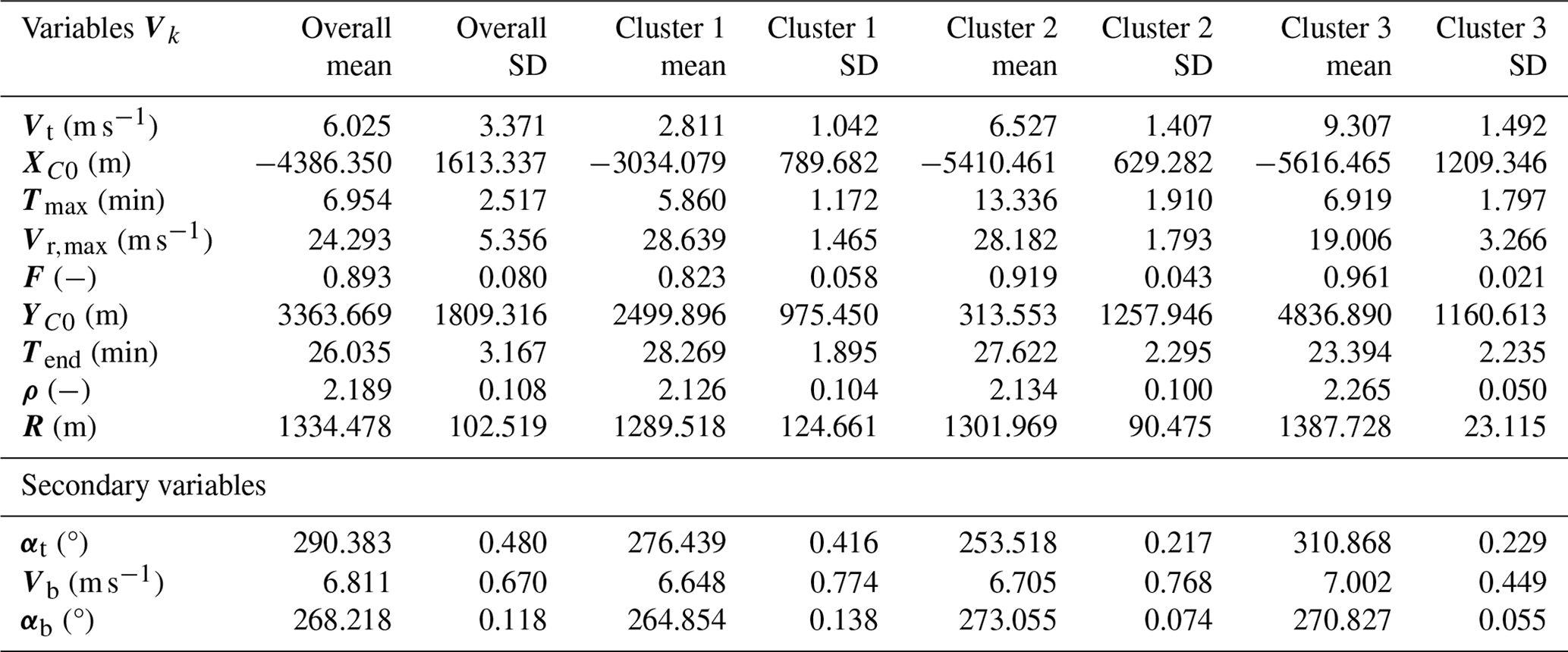
In columns 2–3, the overall mean and the overall standard deviation (SD) are calculated with respect to each variable (primary and secondary). In the other columns, the same calculation was repeated taking into consideration the three clusters. The mean and the SD of the secondary variables α_t and α_b have been calculated using circular statistics (Rao and Sengupta, 2001). To start clarifying the characteristics of the different clusters, Fig. 14 shows the scatterplot and distribution of the touchdown components (X_C0,Y_C0) for all the solutions, partitioned into three clusters. In this figure the center (namely the mean) of each cluster and the location of the touchdown position of the best overall solution are shown. The figure also shows the position of the city of Sânnicolau Mare with a black line. Additionally, on the left and on the top of this figure the histograms of the variable (X_C0,Y_C0) relative to each cluster are shown.

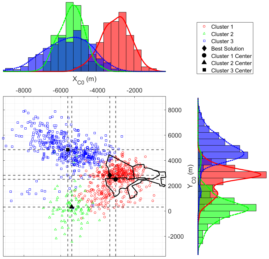
Figure 14 Scatterplot and histogram density distribution for the variables (X_C0,Y_C0). The dark-black line shows the contours of the city of Sânnicolau Mare.

The three clusters appear well separated in terms of touchdown position (X_C0,Y_C0). Since it is very unlikely that the cluster means coincide with one of the solutions present in the dataset, let us define a “cluster solution” as the solution which is the closest to the mean of the cluster across all variables. Accordingly, the cluster solutions, reported in Table 6, will be used to interpret the average features of each cluster. The first row of this table is dedicated to the best solution found by the optimization algorithm (i.e., the one that has the lowest objective function F among all the solutions); the best solution is associated with cluster 1.

Table 6 Best overall solution and representative cluster solutions.

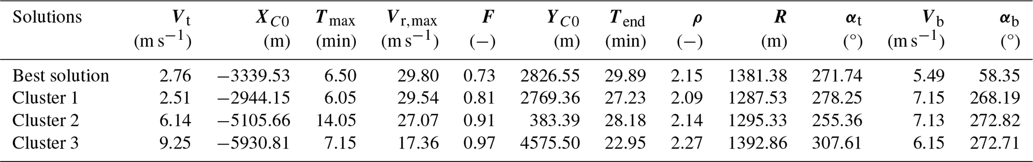
Figure 15 shows the time histories produced by the best solution and the three cluster solutions, in terms of wind velocity (Fig. 15a) and direction (Fig. 15b), compared with the moving-average recorded data. The figure provides a qualitative representation of the goodness of fit between the simulations and the recorded data. The goodness of fit is quantitatively measured by the objective function F. The simulations produced from the best solution and the solution for cluster 1 fit the data better than those of clusters 2 and 3. This is quite obvious since the best solution has the lowest objective function F and is associated with cluster 1, whereas solutions for cluster 2 and cluster 3 have a slightly higher objective function F (refer to column 5 in Table 6).

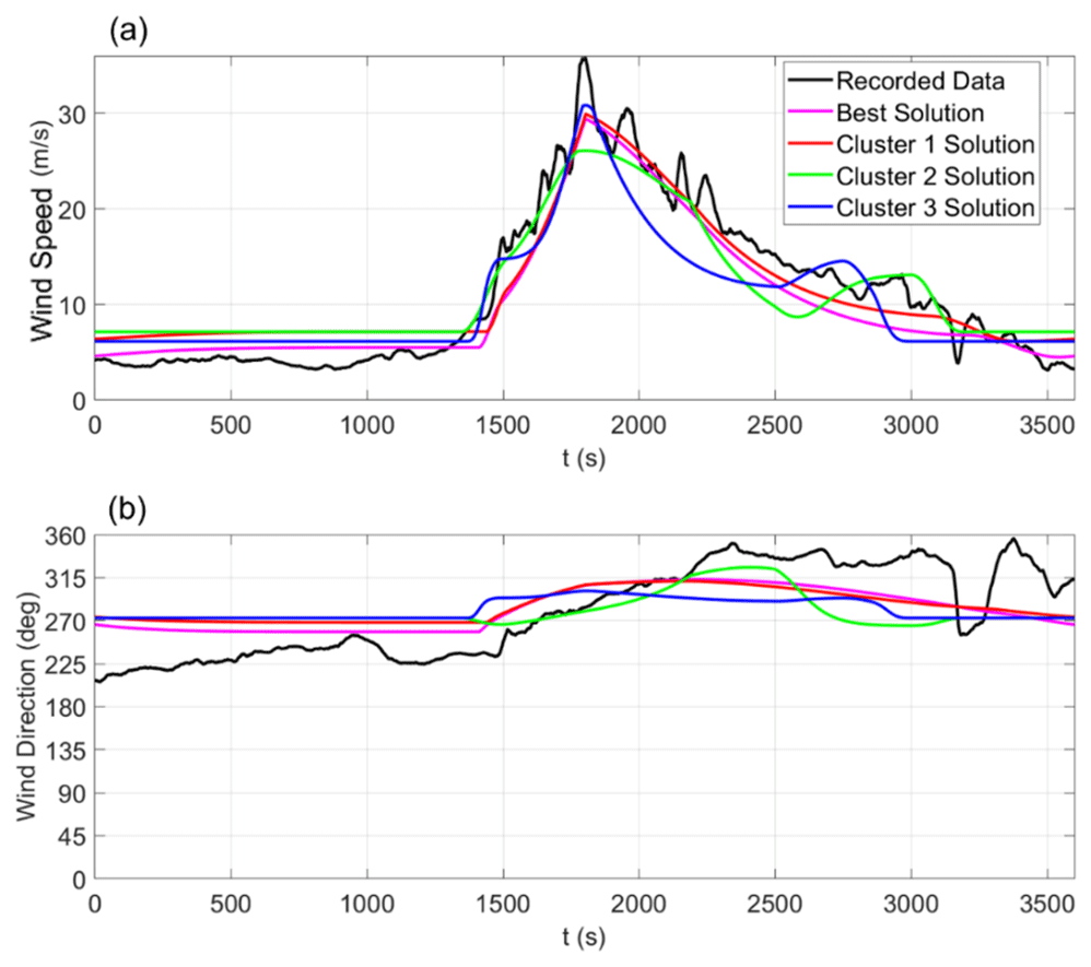
Figure 15 Comparison of the moving-average wind (a) speed and (b) direction obtained from the measurements of the Sânnicolau Mare downburst, along with the best solution and the three cluster solutions.

In order to better understand the nature of the different solutions relative to each cluster, for each solution present in Table 6, the downburst two-dimensional wind velocity is evaluated at the same height of the anemometric station (i.e., at 50 m a.g.l.). Figure 16a–d show for each of the four solutions the wind field reconstruction during the intensification stage of the downburst, while Fig. 16e–h describes the stage of maximum intensity. Note that the time of maximum intensity is different for each cluster according to the corresponding value of T_max reported in column 3 of Table 6.

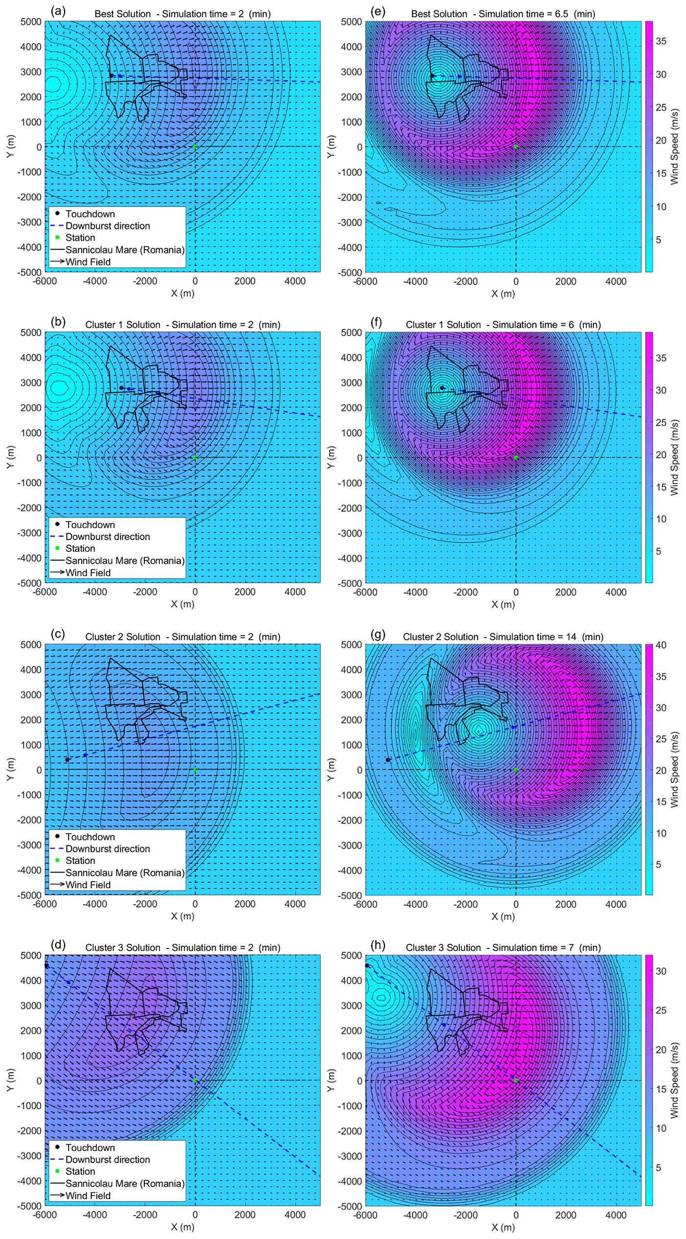
Figure 16 Two-dimensional wind field reconstruction at 50 m a.g.l. Depicted at the intensification stage of the downburst are (a) the best solution and (b–d) solutions for (b) cluster 1, (c) cluster 2, and (d) cluster 3. Depicted at the maximum intensification stage of the downburst are (e) the best solution and (f–h) solutions for (f) cluster 1, (g) cluster 2, and (h) cluster 3.

Cluster 1 touches down very close to the city center and moves slowly eastward; it is characterized by a low value of the downburst translation velocity V_t, with a mean value of 2.8 m s⁻¹ against the overall mean among all clusters, which is 6.0 m s⁻¹. In addition, it has a maximum radial velocity V_r,max higher and overall duration of the downburst event T_end which is longer with respect to the mean values of the other two clusters. The solutions associated with the touchdown of cluster 2 around 2 km southwest of the city propagate northeastward, with higher translation velocities compared to those of cluster 1 and the longest intensification periods T_max overall. The solutions in cluster 3 touch down about 3 km northwest of the city; they move southeastward, with the highest values of downburst translation velocity V_t, but they are the shortest, as the duration of the downburst event T_end is on average 23.4 min, while the overall mean is 26.0 min. They also have the lowest values of maximum radial velocity V_r,max, compensating the high translation velocities. According to these descriptions, it is clear that in the solution space of the model three different solutions exist that can describe similarly of the time series measured at TM_424. The existence of different plausible solutions means that the problem of finding the downburst wind field time–space evolution using a single time series is an underdetermined problem.

The Sânnicolau Mare downburst had a strong impact, causing hail damage to numerous buildings in the town. A damage survey was conducted to assess the affected areas and identify buildings that experienced hail damage during the event. To estimate the extent of the damage, the simulated wind field generated by the analytical model was utilized. By analyzing the wind speeds at various locations, the “footprint” of the simulated damage was determined. This footprint represents the maximum wind speed recorded at different places during the downburst, providing valuable information on the areas most affected by the event. Figure 17a–d depict the complete footprint of the downburst potential damage area for the best solution and the three cluster solutions. In contrast, Fig. 17e–h provide a closer view of the footprints overlaying the simulated maximum wind velocity vectors (indicated by blue arrows) onto the locations of hail damage. The hail damage is represented by vectors pointing orthogonally to the damaged facades (represented by pink arrows). The comparison between the facade damage, which is related to the trajectory of hail transported by the strong downburst-related outflow, and the simulated maximum velocity reveals interesting findings. Specifically, the best solution and solution for cluster 1 exhibit the strongest alignment between the maximum wind velocity vectors and hail damage vectors, particularly in the central part of the city and along the path of the downburst. In contrast, cluster 2 and cluster 3 demonstrate a consistent deviation of the maximum velocity, with cluster 2 deviating northward and cluster 3 deviating southward, relative to the hail trajectories. This observation suggests that the actual downburst event likely followed a pattern more closely resembling cluster 1 rather than the other two potential solutions.

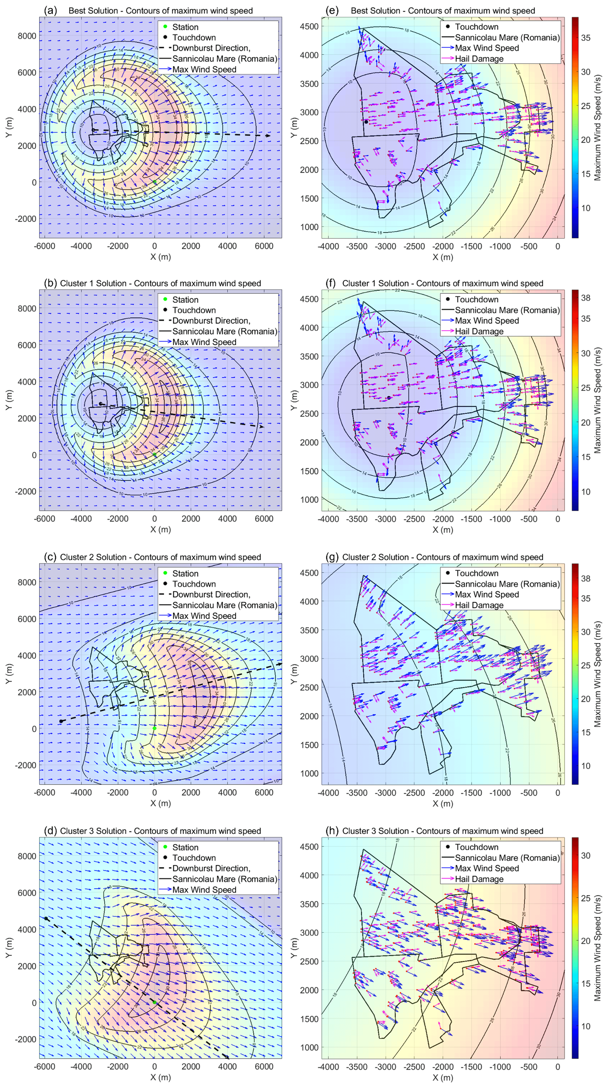
Figure 17 Simulated footprints of the downburst that occurred in Sânnicolau Mare. Footprints for (a) the best solution and (b–d) solutions for (b) cluster 1, (c) cluster 2, and (d) cluster 3. Comparison of hail damage and maximum simulated wind speed for (e) the best solution and (f–h) solutions for (f) cluster 1, (g) cluster 2, and (h) cluster 3.

These observations lead to the conclusion that the optimal (best) solution, which minimizes the objective function F, is the most reliable among all possible solutions. In the current study, this has been achieved through a comprehensive approach involving numerous simulations, specifically tailored to cases where only anemometric data are available, despite having access to additional data types like radar images. This choice was driven by the higher likelihood and frequency of availability of anemometric data in practical scenarios, thus providing a more universally applicable context for the analytical downburst model. The methodology involved conducting a large number of simulations to thoroughly explore the solution space, given the data-limited scenario. Consequently, this approach enabled the extraction of kinematic and geometric parameters of the downburst outflow wind field exclusively from anemometric data.

However, it is important to acknowledge that in scenarios where additional data types such as radar or lidar or other sensors are available, the approach to reconstructing the downburst wind field would differ significantly. In such situations, the availability of more diverse data allows for a more constrained and targeted reconstruction process. By integrating specific parameters from these additional data sources, like storm speed and direction and ABL wind speed and direction, the solution space can be narrowed down more effectively, potentially reducing the number of simulations needed and enhancing the precision of the model.

6 Conclusions

This study focuses on the analysis of solutions obtained by combining an analytical model (Xhelaj et al., 2020) with a global metaheuristic optimization algorithm for the reconstruction of the wind field generated during the Sânnicolau Mare downburst event in Romania on 25 June 2021. The analytical model and optimization algorithm are coupled using the teaching–learning-based optimization (TLBO) algorithm to estimate the kinematic parameters of the downburst outflow. The procedure for this coupling and parameter estimation is described in detail in the study by Xhelaj and Burlando (2022). Therefore, the objective was to analyze the differences among the solutions provided by the optimization algorithm and to assess their physical validity as alternatives to the optimal solution. In the presence of multiple physical sounding solutions, it has been demonstrated that additional data describing the downburst thunderstorm event are necessary to determine which solution best represents reality. To support the analysis a comprehensive damage survey was conducted in collaboration with the University of Genoa (Italy) and the Technical University of Civil Engineering of Bucharest (UTCB) to assess the extent and location of hail damage on buildings in the affected area. This survey, along with the wind speed and direction signals recorded during the downburst event by a telecommunication tower located approximately 1 km from the city, significantly enhances the information available for the reconstruction and simulation of the downburst using the optimization procedure. The analysis of the solutions generated by the optimization algorithm involves multivariate data analysis (MDA) techniques, specifically agglomerative hierarchical K-means clustering (AHK-MC) and principal component analysis (PCA). AHK-MC is used for classifying the solutions into different clusters based on their features, while PCA is employed to determine the importance of the variables in the analytical model for the downburst event reconstruction.

The application of AHK-MC resulted in the identification of three main clusters, each with distinct characteristics, among the 1024 solutions.

• Solutions associated with cluster 1 are characterized by slow storm motion, a small touchdown distance from the city of Sânnicolau Mare, and a long duration of the downburst event. The best overall solution is associated with cluster 1.

• Solutions associated with cluster 2 are characterized by moderate storm motion and a moderate distance of the touchdown from the town of Sânnicolau Mare. These solutions are also characterized by a high duration of the intensification period of the downburst event.

• Solutions associated with cluster 3 are characterized by fast storm motion and a large distance of the touchdown from Sânnicolau Mare. They are also characterized by a low duration of the downburst event and low values of the maximum radial velocity.

The result of the MDA also allows for establishing at least for the case under consideration that the variables of {${\mathit{V}}_{\mathrm{t}},{\mathit{X}}_{C\mathrm{0}},{\mathit{T}}_{\max },{\mathit{V}}_{\mathrm{r},\max },\mathit{F},{\mathit{Y}}_{C\mathrm{0}}$}, which are ordered from the strongest to the weakest, are the more important for the reconstruction/simulation of the downburst event. The remaining variables of {${\mathit{T}}_{\mathrm{end}},\mathit{\rho },\mathit{R}$} have a lower contribution. It is important to observe that the partitioning in the strongest and weakest variables does not represent a general case, since the partition depends on the downburst case under study.

Finally, the comparison between the facade damage, which is related to the trajectory of hail transported by the strong downburst-related outflow, and the simulated maximum velocity shows that the best solution and solution for cluster 1 seem to have a “good” overlap between maximum wind velocity vectors and hail damage vectors. Considering the solutions of cluster 2 and 3, it seems that the match between maximum wind velocity vectors gradually decreases, with the worst case represented by the solution for cluster 3. These observations allow for concluding that the optimal solution, that is, the one that minimizes the objective function F, is the best with respect to the other three cluster solutions, also from the point of view of the damage analysis. As a result, for the specific case being examined, relying on the best overall solution provided by the optimization algorithm appears to yield promising results for reconstructing the downburst wind field. Obviously, an analysis of this type, conducted on several downburst events, will be better able to confirm this statement.