Comparison of debris flow observations, including fine-sediment grain size and composition and runout model results, at Illgraben, Swiss Alps

Debris flows are important processes for the assessment of natural hazards due to their damage potential. To assess the impact of a potential debris flow, parameters such as the flow velocity, flow depth, maximum discharge, and volume are of great importance. This study uses data from the Illgraben observation station in the central Alps of Switzerland to explore the relationships between these flow parameters and the debris flow dynamics. To this end, we simulated previous debris flow events with the RAMMS::Debrisflow (Rapid Mass Movement Simulation::Debrisflow) runout model, which is based on a numerical solution of the shallow water equations for granular flows using the Voellmy friction relation. Here, the events were modelled in an effort to explore possible controls on the friction parameters μ and ξ, which describe the Coulomb friction and the turbulent friction, respectively, in the model. Additionally, sediment samples from levee deposits were analysed for their grain size distributions (14 events) and their mineralogical properties (4 events) to explore if the properties of the fine-grained matrix have an influence on the debris flow dynamics. Finally, field data from various debris flows such as the flow velocities and depths were statistically compared with the grain size distributions, the mineralogical properties, and the simulation results to identify the key variables controlling the kinematics of these flows. The simulation results point to several ideal solutions, which depend on the Coulomb and turbulent friction parameters (μ and ξ, respectively). In addition, the modelling results show that the Coulomb and turbulent frictions of a flow are related to the Froude number if the flow velocity is < 6–7 m s⁻¹. It is also shown that the fine-sediment grain size or clay-particle mineralogy of a flow neither correlates with the flow's velocity and depth, nor can it be used to quantify the friction in the Voellmy friction relation. This suggests that the frictional behaviour of a flow may be controlled by other properties such as the friction generated by the partially fluidised coarse granular sediment. Yet, the flow properties are well-correlated with the flow volume, from which most other parameters can be derived, which is consistent with common engineering practice.

1 Introduction

1.1 Debris flows and parameters controlling their velocity and runout

Debris flows are rapid mass movements consisting of water-saturated and poorly sorted debris with a large range of grain sizes. Debris flows tend to develop one single surge or a suite of multiple surges with steep coarse-grained fronts. Their motion is driven by gravity and resisted by friction within the flow and at the boundary with the channel bed (Iverson, 1997). The boulder-rich front is then followed by a tapering body where the pore fluid pressures are large, often exceeding the hydrostatic pressure (Iverson, 1997; McArdell et al., 2007). In the frontal part, larger particles tend to ascend in the debris flow body due to particle collisional stresses, thereby building a coarse-grained top layer (Johnson et al., 2012), which travels somewhat faster than the flow front itself, delivering the coarse sediment to the front. Accordingly, the coarser-grained particles along with some of the fine sediment present at the surface of the flow tend to accumulate in the surge head and are deposited laterally in levees just a few metres behind the front (Johnson et al., 2012).

Recently, de Haas et al. (2015) conducted experiments to investigate how the grain size distribution and water content influence the velocity of a debris flow. They found that a higher clay content tends to result in an increase in both the velocity and the runout distance of such flows. However, if the clay content becomes too large, then the velocity decreases due to the higher viscosity of the fluid. This relationship should also be applicable to the silt fraction because clay and silt particles are a part of the fluid, while grains larger than silt contribute to the solids of a debris flow (Iverson, 1997). The experiments of de Haas et al. (2015) also showed that a large gravel content in the flow front leads to a strong frictional resistance, which in turn reduces the flow velocity. In addition, a large gravel content results in a larger pore water diffusivity, which reduces the pore pressure in the flow and contributes to a further reduction in the flow velocity. On the other hand, a low gravel content leads to lower collisional forces, which might also lead to a relatively low flow velocity. Furthermore, also according to the experiments by de Haas et al. (2015), the water content, the velocity, the volume, and the runout distance of a debris flow are positively correlated to each other. Based on a combination of experimental and field data, Hürlimann et al. (2015) came to the same conclusions, and they additionally found that an increase in the clay content generally leads to a reduction in the runout distance. Indeed, the absorption of water in swelling clay minerals has the potential to result in an increase in the cohesion of a flow, which in turn could cause a reduction in the flow velocity and the runout distance. Finally, using laboratory experiments, Kaitna et al. (2016) documented that a relatively high fraction of fine-grained material tends to occur in flows with excess pore fluid pressures. In addition, these authors mentioned that such flows were characterised by low fluctuations in normalised fluid pressures and normal stresses, and the experiments showed that the shear stresses were concentrated at the base of the flow. Based on the conclusions of the aforementioned authors, we expect to see a dependency of the flow properties in Illgraben and the granulometric composition of these flows (Uchida et al., 2021), and we anticipate that the flow velocity is negatively correlated with the relative abundance of the finest-grained particles.

The mineralogical composition of a flow is a further parameter, which has the potential to impact the rheology and thus the flow velocity and runout distance of debris flows, yet these relationships have largely been overlooked in the literature. In particular, because clay minerals are important constituents of the fine-grained fraction of these flows, they have the potential to regulate the pore fluid pressure and the stress state through their ability to absorb water in their crystal structure (Di Maio et al., 2004). This is mainly the case for swelling clay minerals such as those of the smectite group (Di Maio et al., 2004), where the pore fluid composition has a large influence on the volume and the shear strength of these minerals (Chatterji and Morgenstern, 1990; Di Maio, 1996). Because shear stresses within a flow are a direct consequence of the friction between the particles and the fluid phase and since the friction properties directly influence the propagation of a debris flow (see Sect. 1.2), we anticipate the occurrence of a direct relationship between the velocity and runout distance of debris flows and the mineralogical composition of the fine-grained matrix.

1.2 Physically based models describing debris flow processes and the goal of the paper

There are several rheological models or flow resistance relationships describing the behaviour of debris flows such as the flows' velocities, runout distances, and frictional properties (e.g. Allen, 1997; Rickenmann, 1999; Naef et al., 2006). One commonly used approach is the Voellmy friction relation (Voellmy, 1955; Salm et al., 1990; Salm, 1993; Christen et al., 2012), which is also implemented in the RAMMS::Debrisflow (Rapid Mass Movement Simulation::Debrisflow) software, a software package used to simulate debris flow runout (see Sect. 3.2). In the Voellmy friction equation, the frictional resistance of a flow S [Pa] is composed of the sum of two friction terms: (i) a dry Coulomb-type friction term, referred to as Coulomb friction, which describes the frictional resistance between the debris flow and the channel bed and mainly depends on the flow depth, and (ii) a drag or viscous turbulent friction term, which describes the turbulent frictional resistance and mainly depends on the dynamic pressure and thus on the velocity of the flow. These components are characterised by the coefficients μ and ξ, which control the values of the Coulomb and the turbulent frictions, respectively (Christen et al., 2012). Optionally, cohesion stresses can be included in an extended Voellmy friction equation (Bartelt et al., 2015; Berger et al., 2016). Because this additional cohesion term has rarely been used in engineering practice and is apparently relatively small (Berger et al., 2016), it was neglected herein, and the friction equation takes the following form:

$$\begin{array}{}\text{(1)}& S=\mathit{\mu }N+{\displaystyle \frac{\mathit{\rho }g{v}^{\mathrm{2}}}{\mathit{\zeta }}},N=\mathit{\rho }gh\cdot \cos \left(\mathit{\phi }\right),\end{array}$$

where S is the frictional resistance [Pa], ρ the density of the debris flow, h the flow height (or flow depth), g the gravitational acceleration, φ the slope angle of the channel bed, and v the velocity of the flow.

A simplified approach to characterise a debris flow is the Froude number, which describes the ratio between the inertial and the gravitational forces:

$$\begin{array}{}\text{(2)}& Fr={\displaystyle \frac{v}{\sqrt{gh}}},\end{array}$$

where Fr is the Froude number, v the velocity of the flow, g the gravitational acceleration, and h the flow height (Hübl et al., 2009; Choi et al., 2015).

As mentioned above, the velocity and runout distance of debris flows are likely to depend on the frictional resistance in such mass movements. This friction, in turn, can be characterised by two coefficients, μ and ξ, in the Voellmy friction relation, Eq. (1). Because we anticipate that the mineralogical and granulometric composition of the fine-grained matrix has an influence on the properties of such flows (see Sect. 1.1), we expect to identify a relationship between the frictional properties, velocity, and grain size and mineralogical composition of a flow. Here, we test and explore these hypotheses using in situ data collected at the Illgraben debris flow monitoring station situated in the Central European Alps (Fig. 1), and we evaluate the data with the results of a numerical runout model referred to as RAMMS. Upon combining field data with modelling results, we aim at identifying those parameters that have the largest control of the dynamic properties of the debris flows at Illgraben.

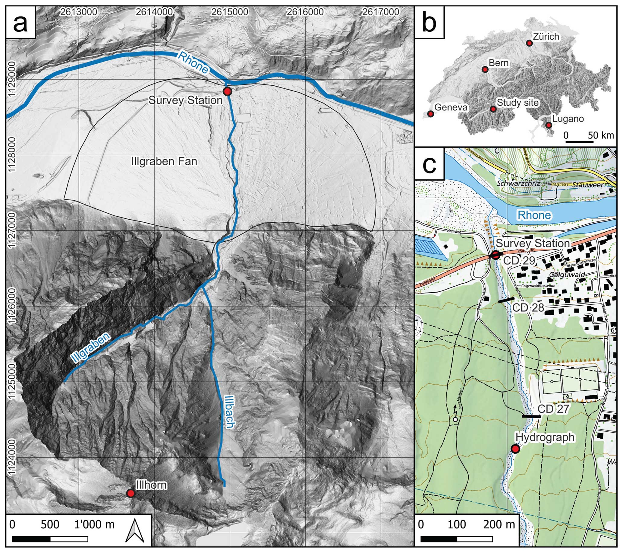
Figure 1 (a) Overview of the topographic situation around Illgraben showing the Illgraben system with its river network consisting of Illgraben, Illbach, and the Rhône River. (b) Overview map of Switzerland with the location of the study site. (c) Detailed topographic map of the Illgraben reach along which the RAMMS simulations have been conducted. It shows the location of the input hydrograph, which was used as the starting position for the modelling. The three check dams (labelled with “CD” in the figure) and the location of the survey station below Pfynstrasse are displayed in this figure. The background is provided by the swissALTI3D and the Swiss Map Raster 10 (Swisstopo, 2022).

2 Study site and setting

The Illgraben catchment is located in the Valais region in western Switzerland (Fig. 1). It extends from the summit of Illhorn (2716 m a.s.l.) to the outlet of Illgraben into the Rhône River (610 m a.s.l.). The total area of about 9.5 km² consists of the Illgraben basin, which has a spatial extent of 4.6 km², and the Illbach tributary catchment covering 4.9 km² (Fig. 1a). The Illgraben basin has been very active and has generated several debris flows each year (Schlunegger et al., 2009; McArdell and Satori, 2022). The rates of sediment discharge in Illgraben have been exceptionally high for Alpine standards (Berger et al., 2011a). Several studies showed that the erosion rates and the numbers and extents of debris flows strongly depend on hydro-climatic parameters such as the average annual temperature and the precipitation rates (Bennett et al., 2013; Hirschberg et al., 2019, 2021a, b). The highly fractured bedrock (Bumann, 2022), belonging to the Penninic nappe stack (Gabus et al., 2008), consists of massive-bedded limestones, quartzites, and Triassic schists with dolobreccia interbeds. Schlunegger et al. (2009) considered these lithologies to be the main source of the silt and clay fraction that constitute the matrix of the debris flow deposits. Based on a petrographic analysis of the debris flow deposits, these authors also identified two distinct sediment sources in Illgraben where bedrock lithologies with different petrological properties are exposed. These are (i) a heavily fractured and foliated suite of gneisses and schists, which are exposed on the southern flank of Illgraben, and (ii) a vertically plunging succession of limestones, dolomites, and cellular dolomites, which make up the northwestern flank of Illgraben (Fig. 1). The material from these two sources is very well-mixed in response to repeated deposition and remobilisation of sediment within the catchment (Schlunegger et al., 2009). The sediment cascade has been subject to seasonal variations, where smaller debris flow events are associated with net sediment accumulation in the channel, while large flows can entrain sediment up to several times their initial mass along their flow paths (Berger et al., 2010; Berger et al., 2011a, b; Schürch et al., 2011).

Grain size analyses conducted on samples from the channel bed and debris flow deposits indicated sand contents of 35 %–40 % and clay contents of < 5 % (Hürlimann et al., 2003; Schlunegger et al., 2009; Uchida et al., 2021). In the Rhône valley, an alluvial fan has formed, covering an area of 6.6 km² (Schürch et al., 2016). The channel on the fan has a U-shaped cross-sectional geometry with a base that is about 5–10 m wide. For the lowermost 2 km, the gradient of the Illgraben channel ranges from about 7 % to 18 % (measured over a length of 50 m) with a mean of about 8 % (Schlunegger et al., 2009). Thirty-one check dams with vertical drops of up to several metres were constructed along the lowermost 4.8 km of the channel to prevent the flows from further incising into the substratum (McArdell et al., 2007; Badoux et al., 2009). A debris flow monitoring station, situated on the lower fan ca. 200 m upstream of the confluence with the Rhône River, was installed in the year 2000 and has been operated by the Swiss Federal Institute for Forest Snow and Landscape Research (WSL) since then (Hürlimann et al., 2003; Badoux et al., 2009). At the survey site (Fig. 1c), the measured parameters include frontal velocity, flow depth, bulk density, maximum discharge rate, volumes, and normal and shear force (McArdell et al., 2007; McArdell, 2016). The related values are presented in the openly accessible database of the WSL (McArdell et al., 2023), and the data were collected using the methods presented in Sect. 3.1. On average, three to five debris flows have been registered by the measuring station every year. They have generally occurred during intense rainstorms between May and October (e.g. McArdell et al., 2007).

3 Methods

Using data collected in the field (Sect. 3.1), we explored how the frictional properties of a debris flow influence the behaviour (flow depth and velocity) of such a flow through modelling with RAMMS (Sect. 3.2). We then tested whether the grain size distribution (Sect. 3.3) and the mineralogical composition of the debris flow material (Sect. 3.4) have an influence on the flow velocity.

3.1 Surveys of debris flows

Many of the in situ measurements of the debris flow properties at Illgraben have been accomplished with a force plate that is installed in the channel beneath a bridge ca. 200 m upstream of the confluence with the Rhône River (survey station; see Fig. 1c). At that survey site, information on (i) the velocity, (ii) the flow depth, (iii) the mean bulk density, (iv) the duration of individual debris flows, and (v) the volumes of each flow has been determined in the past years by the WSL (e.g. McArdell and Sartori, 2021; de Haas et al., 2022; Belli et al., 2022; McArdell et al., 2023). As outlined in McArdell et al. (2007) and Schlunegger et al. (2009), the force plate is a horizontal 8 m² steel structure, which is installed flush with the riverbed just on the top of the concrete check dam. The plate is equipped with normal and shear force transducers. The flow depth is estimated using either a laser or a radar unit. Because the radar data are biased by an unpredictable smoothing of the flow surface, we favoured the use of the laser data for further calculations. Based on information about the flow depth and the normal force, it was possible to determine the bulk density of a flow as it moves on the plate itself. The volume of each flow was then calculated as the product between the velocity and the cross-sectional area, and this product was integrated with the flow's duration (McArdell et al., 2023). The frontal velocity is determined using the travel time of the flow front over the reach upstream of the force plate (between check dams 27 or 28 and 29; Fig. 1c and Hürlimann et al., 2003). Table S1 in the Supplement presents a list of parameters which were measured at the Illgraben monitoring site, and Fig. S1 displays screenshots from video recordings of selected debris flows.

3.2 Numerical modelling using RAMMS

We explored, through modelling using RAMMS, how the frictional properties of a debris flow influence its behaviour such as flow depth and velocity. The RAMMS model was developed by the Swiss Federal Institute for Forest, Snow and Landscape Research, WSL (WSL, 2022). It is based on the two-parameter Voellmy-fluid model (Christen et al., 2012; Bartelt et al., 2015), which describes the friction in the 2D depth-averaged equations of motion deviated for granular flows. We justify the selection of such an approach because in an independent modelling study (FLATModel) calibrated with field data (Medina et al., 2008), the Voellmy-fluid formula (Eq. 1) has been proven to reproduce the dynamics of debris flows (flow velocity, erosion pattern in the channel, and aerial extension of the flow in the accumulation zone) reasonably well. A major challenge for modelling is the choice of the input friction coefficients. In particular, if the simulation cannot be calibrated with data that were collected from a previous well-documented event (Christen et al., 2012; Deubelbeiss and Graf, 2011), the input parameters have to be estimated. Because model results such as the velocity, the runout distance, and the flow depth are sensitive to the friction parameters μ and ξ (Bartelt et al., 2015; Christen et al., 2012), we iteratively changed the values of these coefficients (Tables S2 and S3) until we found, for each event, the best fit between the simulation results and the observations.

The Coulomb friction coefficient μ is sometimes expressed as the tangent of the internal shear angle (WSL, 2022). According to Salm (1993), an internal movement parallel to the slope is only possible if the internal shear angle is smaller than the slope angle. Consequently, the value of μ should be smaller than the tangent of the channel slope angle. For a minimum slope angle of 7 % (4°), μ should thus be smaller than 0.07. Therefore, for every debris flow event, we conducted several simulations (between 12 and 43, Tables S2 and S3) with μ varying from 0.01 to 0.06, and we modified the ξ parameter to minimise the z value, which is explained with Eq. (3) below. This resulted in μ–ξ pairs with lowest z values and thus the best fits between the model results and observations (such as the flow velocity v and the flow depth h). Please see Tables S2 and S3 for information about the number of modelling runs, intervals between the μ and ξ values, and other input parameters that we used for modelling.

We employed the “hydrograph” input option of RAMMS to characterise the debris flows in the model. Upon modelling, the hydrograph input was placed ca. 500 m upstream of the survey site (check dam 27; see Fig. 1c). It was allowed for erosion to occur along the entire channel (Frank et al., 2015, 2017) except at the check dams. Similar to the surveys in the field (Sect. 3.1), the model velocity was calculated using the travel time between check dams 28 and 29 (Fig. 1c). The modelled flow depth values used herein were obtained as the average of the measurements that were conducted at four points along a cross section at check dam 29.

The use of RAMMS requires a digital elevation model (DEM), event volume, and peak discharge. The drone-based DEM, which is based on a survey conducted on 10 August 2021 (de Haas et al., 2022), was used for all simulations. However, this high-resolution DEM did not cover the section of the channel between the survey station and the Rhône River (Fig. 1c). Therefore, in order to extend the area towards the confluence with the Rhône River, the photogrammetry DEM, which has a resolution of 0.1 m, was combined with an existing 0.5 m lidar DEM (Swisstopo, 2022) using the software QGIS. Here, we resampled the drone-based DEM to achieve the same resolution as the lidar DEM of Swisstopo (i.e. 0.5 m) so that the two datasets could be combined. The DEM of the short, concrete channel section beneath the road bridge had to be reconstructed manually because it was not possible to image the topography below the bridge. In addition, a filter (Serval raster editing tools, version 3.10.2) was applied to the channel bed to smoothen the bed surface. This was done because a large local change in the topography (such as a boulder) can induce strong vertical accelerations in RAMMS (and other models that are based on the depth-averaged equations of motion), which can lead to unrealistically large (or small) local flow depths.

Finally, we introduced a dimensionless z value to describe the deviation in the simulated velocity v_sim and flow depth h_sim from the measurements in the field:

$$\begin{array}{}\text{(3)}& z=\sqrt{{\left({\displaystyle \frac{v_{\mathrm{sim}}-v_{\mathrm{measured}}}{v_{\mathrm{measured}}}}\right)}^{\mathrm{2}}+{\left({\displaystyle \frac{h_{\mathrm{sim}}-h_{\mathrm{measured}}}{h_{\mathrm{measured}}}}\right)}^{\mathrm{2}}}.\end{array}$$

We thus explored how the model input parameters (μ and ξ values) affect the modelled velocity and depth values of a flow. We then compared the model results with the surveyed velocities and depths of each flow using Eq. (3), which we implemented in the software MATLAB R2021b.

3.3 Grain size distribution

For most of the debris flows that occurred in the years 2019, 2021, and 2022, at least one sediment sample of 1.5 to 3 kg was taken from the levee deposits at the same site labelled as “survey station” in Fig. 1c (2^′614^′973 m E, 1^′128^′842 m N in Swiss coordinates). We collected the material from underneath the bridge to prevent effects related to grain-size-dependent erosion by rainfall. We selected the levee deposits for three reasons. First, according to our experience, the levee deposits can better be attributed to a specific event than other sediments of a debris flow. Second, the levee deposits are those sediments of a debris flow that most clearly record the granulometric composition of the surge head, as our observations on video recordings have shown. Third, it is the surge head which exerts the greatest control on the dynamics of a debris flow (McArdell et al., 2007; Johnson et al., 2012). Accordingly, upon collecting material from levee deposits, we are likely to analyse sediments with the highest potential to provide information that allows us to understand the dynamics (e.g. flow depth and velocity) of past debris flows. Yet we acknowledge that this material is more likely coarser-grained than the sediments in the tail of such a flow (McArdell et al., 2007).

In the laboratory, all of the collected material was processed following the state-of-the-art protocol (SN 670 004-2b NA norm), which was established at the Bern University of Applied Sciences (Burgdorf). Following this protocol, the material was first dried and then sieved to a minimum particle size of 0.5 mm using a set of seven sieves, each of which has a defined mesh size: 31.5, 16, 8, 4, 2, 1, and 0.5 mm. Subsequently, a slurry analysis was carried out of the material < 0.5 mm using a hydrometer. The goal of this task was to determine the particle size distribution between 0.001 and 0.1 mm. Finally, the grain size distribution of the remaining material between 0.063 and 0.5 mm was determined by wet sieving. During this task, we used three sieves where the mesh size was 0.25, 0.125, and 0.063 mm. The grain size distribution was truncated at 16 mm so that the entire sample is at least 100 times the mass of the largest particle (e.g. Church et al., 1987). We note, however, that particles larger than 16 mm do occur on the levee deposits and we did sample such material in the field. However, we were not able to consider this fraction due to technical limitations in our laboratory and practical limitations on the mass of the sample necessary for analysis.

3.4 Powder X-ray diffraction (XRD)

We hypothesise that clay minerals influence the pore pressure of a flow (Barshad, 1952), which in turn could influence its mobility (McArdell et al., 2007). We expect such a control because swelling clays tend to absorb water in their crystal structure. The result is an increase in the viscosity of the flow, thereby reducing the dissipation of the fluid pore pressure. To test this hypothesis, the mineralogical properties of some debris flow samples were measured using standard powder X-ray diffraction (XRD) at the Institute of Geological Sciences of the University of Bern. For this purpose, four samples were chosen from fast- and slow-velocity flows as well as from deposits where either the coarse-grained or the fine-grained fractions dominate in the analysed grain size spectrum. To this end, the grain size fraction < 0.063 mm, which was already extracted during the steps outlined above, was analysed with powder XRD. Subsequent milling with a vibratory disc mill (Retsch RS 200) and a McCrone XRD-mill reduced the particle sizes to the sub-micrometre scale. Corundum powder was added as a standard to the samples, and the samples were measured with the X-ray diffractometer X'Pert Pro MPD with Cu radiation. Because this step did not include a determination of the mineralogic composition of the clay minerals, a slightly different approach had to be employed. Here, we used the same initial material, but it was only milled with the vibratory disc mill. The powder was then mixed with a dispersant (0.1 molar NH₃) to achieve a homogeneous suspension. The clay particles were separated in an Atterberg cylinder. The particles still in suspension after 15 h were extracted using a centrifuge. The extracted clay particles were then cleaned with HCl, CaCl₂, and deionised water. To distinguish between the different clay minerals, three sample holders were either air-dried, treated with ethylene glycol, or heated to 400 and 550 °C before measuring with the X'Pert Pro MPD with Cu radiation. The final processing of the data was carried out with the software TOPAS (Coelho, 2018), which uses a Rietveld structure refinement technique (Rietveld, 1969).

4 Results

4.1 Survey results

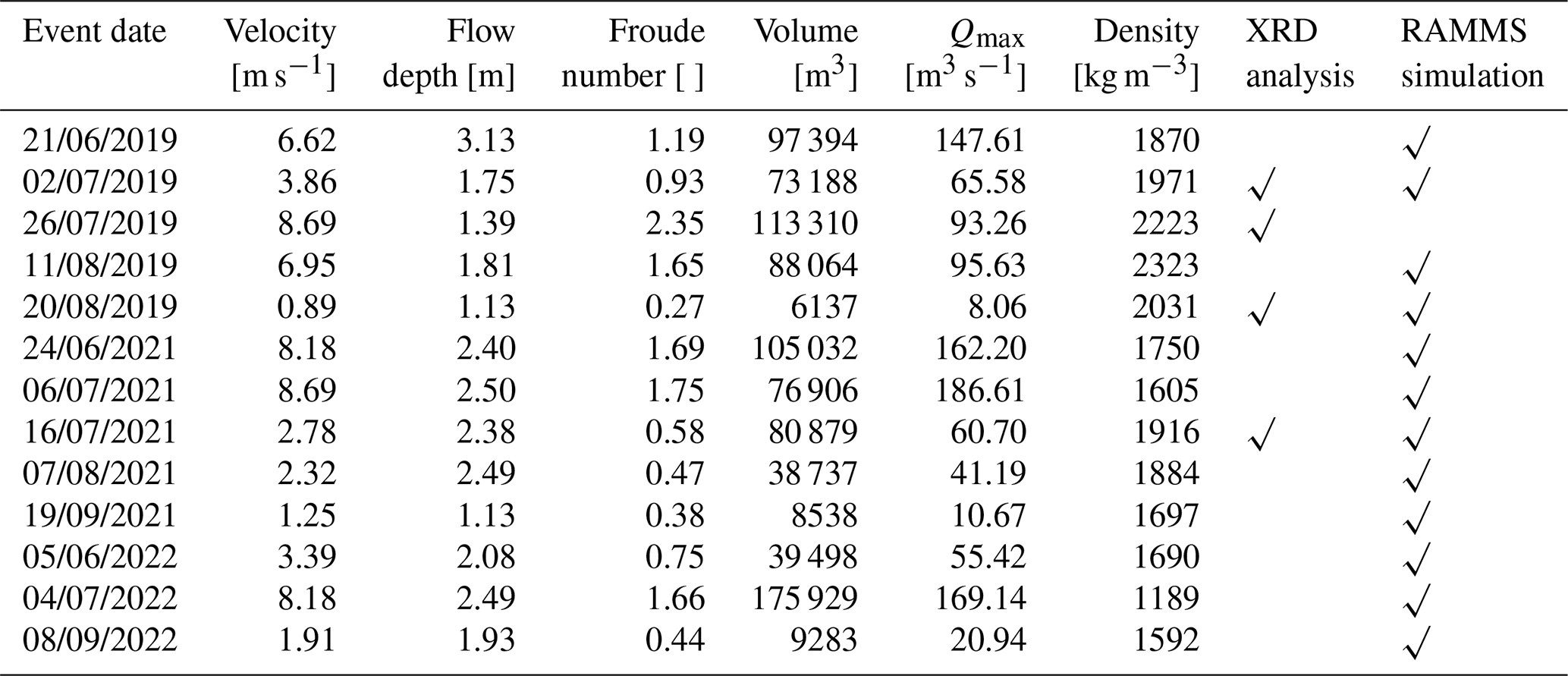
A total of 13 events from 2019, 2021, and 2022 were analysed (Table S1, Table 1). The measured flow velocities varied by 1 order of magnitude from 0.89 to 8.69 m s⁻¹. The maximum flow depths ranged from 1.13 to 3.13 m, and the Froude numbers spanned the interval between 0.27 and 2.35, pointing towards considerable differences in the dynamics of these flows. The total volumes reached a maximum of ca. 176 000 m³, and the maximum discharge rate was ca. 190 m³ s⁻¹. The measured density ranged from 1189 to 2323 kg m⁻³, and the corresponding volumetric water contents were between ca. 20 % and 90 %.

Table 1 Measured and analysed debris flow events from 2019, 2021, and 2022. Velocity, flow depth, volume, maximum discharge (Q_max), and density are the results of direct measurements at the monitoring station in Illgraben (Fig. 1c). The Froude number was derived from these measurements. The last two columns show for which events XRD analyses and RAMMS simulations were performed. The event of 26 July 2019 could not be simulated due to the high Froude number.

4.2 Numerical modelling with RAMMS

As mentioned above, we iteratively changed the μ and ξ friction values upon modelling until we found a best fit between the modelled and observed flow velocity and flow depth of each flow (Tables S2 and S3). Because the latter properties of a debris flow (velocity and depth) can be characterised by the Froude number (defined by Eq. 2), we first describe the dependency of the modelled flow pattern on the Froude number, which itself is calculated using the flow depth and velocity data of the field survey (Table 1). Please note that in this context, Eq. (2) predicts that changes in the flow velocity have a larger impact on the Froude number than variations in flow depth. The simulations showed that RAMMS produces reasonable results (e.g. Fig. 2) for Froude numbers up to about 1.75 (Table 1). For larger values (e.g. flows with large flow velocities), the simulations predict the occurrence of standing waves at the debris flow front, which, however, have not been observed at Illgraben. Therefore, no simulations were possible for the event on 26 July 2019 because this flow was characterised by a Froude number of 2.35. We acknowledge that roll waves, which could correspond to the standing waves simulated by RAMMS, do occur in a debris flow, but such waves are mainly observed in the debris flow body and not at the bouldery front.

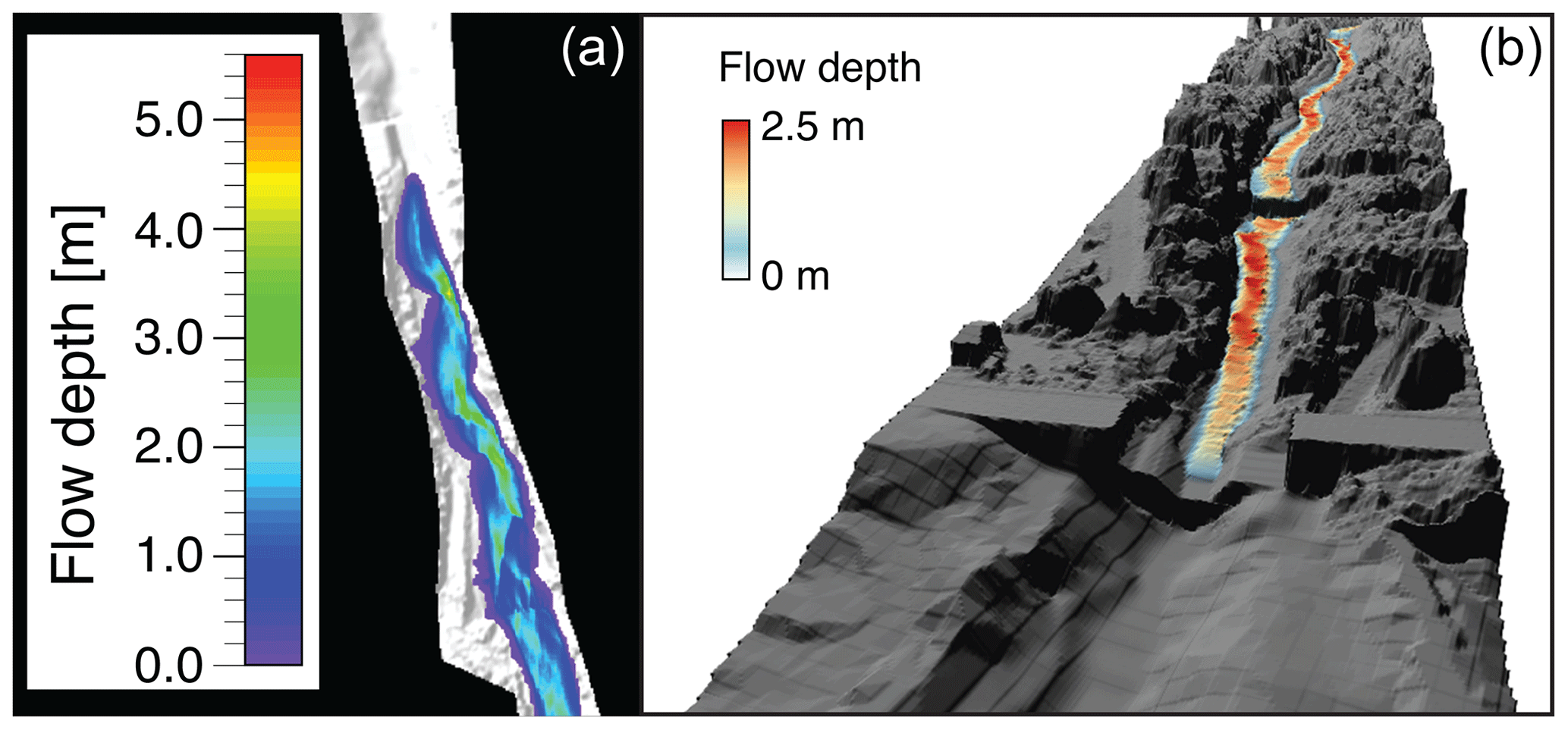
Figure 2 Example of simulated flow depths. The image on the left shows flow depths in a 2D view provided by the RAMMS software. The image on the right shows a 3D view of the debris flow projected on a hillshade model using the software QGIS.

The model results show that more than one best-fit μ–ξ pair is possible for successfully reproducing the observed velocity and depth of a flow (Table S4). Yet, on average, the lowest z value is calculated for the μ–ξ pair with μ= 0.01, followed by the pairs with μ = 0.02 and μ= 0.05. These values and patterns are consistent with the results of other analyses of debris flows conducted with RAMMS and applied to observations in, for example, the Alps (see Mikoš and Bezak, 2021, for an overview of related papers), the Himalayas near Luzhuang in China (Jianjun and Zhang, 2019; μ and ξ values of 0.07 and 1500 m s⁻², respectively), and the coastal region in the vicinity of the Western Ghats in India (Abraham et al., 2021; μ and ξ values of 0.01 and 100 m s⁻², respectively). In addition, Simoni et al. (2012) found that RAMMS successfully reproduced the maximum observed runout distances of debris flows in the Italian Alps for μ values close to the energy gradient of the debris flow channel (which is the tangent of the surface slope). Our modelling results support these inferences and additionally show that the modelled μ and ξ relationships show a strong dependency on the corresponding Froude numbers calculated from the field data (Fig. 3 and Tables S4 and S5). Besides, for a given μ value, the RAMMS models predict that the ξ values increase with the Froude number. Such an increase is more obvious for large than for small μ values (Fig. 3; see also Table S5).

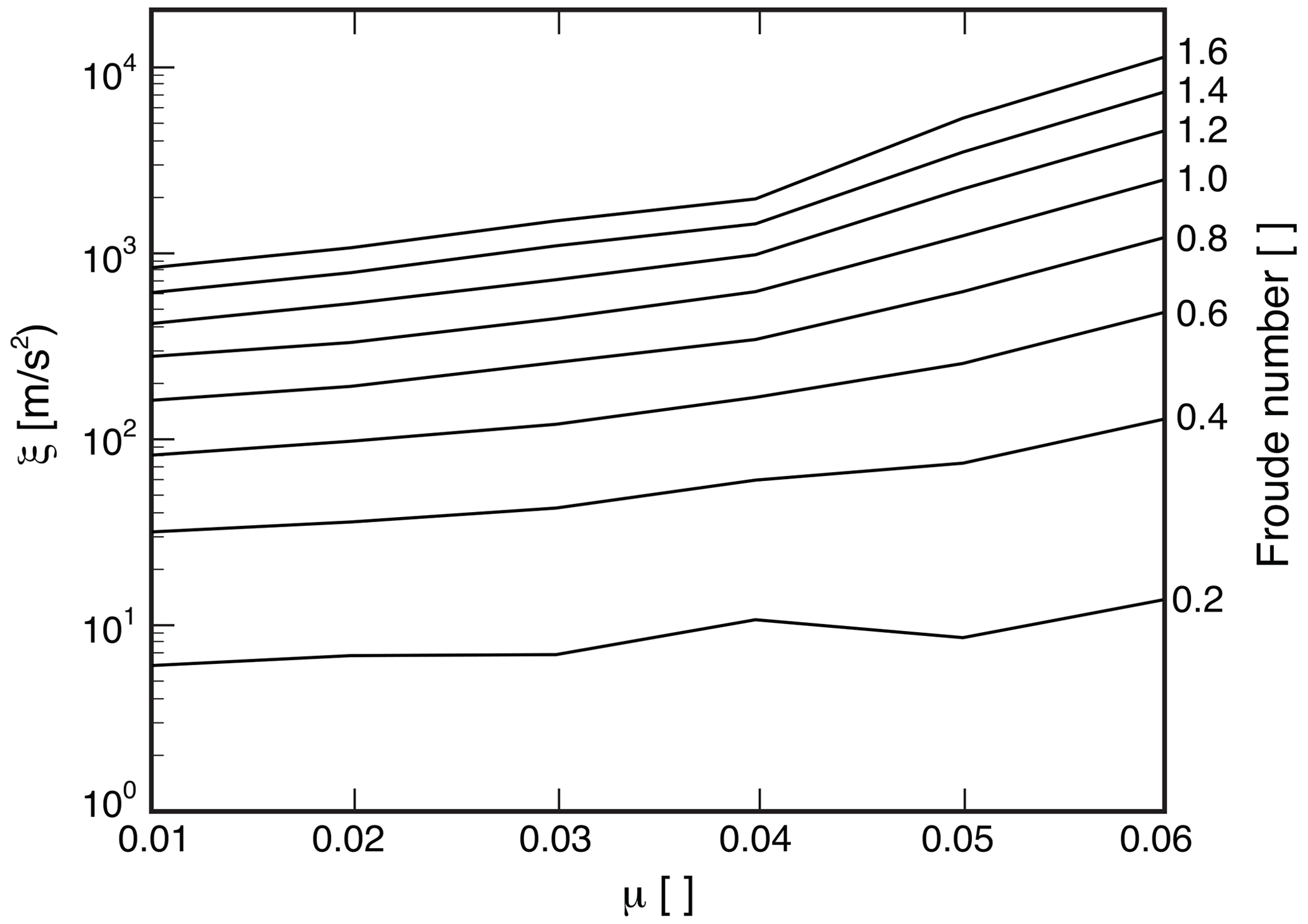
Figure 3 Modelled μ–ξ pairs, which result in a best fit between the observed and the modelled debris flow parameters. These latter values, in turn, appear to depend on the Froude numbers (based on measurements in the field; see Table 1) of the corresponding debris flow events.

Figure 4 illustrates that upon modelling, the relative contribution of the Coulomb friction to the total friction increases with the flow velocity, and it shows that this contribution is greater for large μ values than for small ones. In particular, while the percentages of the Coulomb friction are in the range of ca. 20 % for a μ value of 0.01 and a flow velocity of < 1 m s⁻¹, they increase to > 90 % for a larger μ value of 0.06 and a flow velocity of > 8 m s⁻¹.

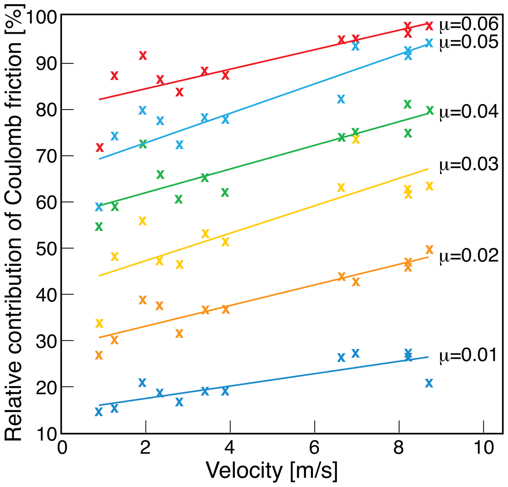
Figure 4 Correlations between the relative contribution of Coulomb friction to the total friction in percentages (y axis) and the velocity of a debris flow (x axis) for different μ values. The data points refer to best-fit simulations only. The lines are first-order polynomial least-squares-fitted trend lines.

The relationships elaborated above are further detailed in Fig. 5, which documents the dependency of the friction properties (Coulomb and turbulent frictions) of a flow on its velocity and the corresponding Froude number. Note that for this analysis, we only considered the results of the best-fit simulations of each flow. Accordingly, rapid debris flows with high Froude numbers tend to be characterised by large Coulomb friction, while slower debris flows are simulated more reliably with rather low Coulomb friction (Fig. 5a, b). Conversely, flows with a slow velocity tend to have larger turbulent friction and are characterised by a low Froude number, whereas the turbulent friction tends to be low for flows with high velocity and a high Froude number (Fig. 5c, d). However, we note that the aforementioned relationships between flow velocity, Froude number, and turbulent and Coulomb frictions break down for flows that are more rapid than ca. 6–7 m s⁻¹ (Fig. 5). Similar to the event on 26 July 2019, these flows are characterised by Froude numbers that are much larger than 1 (Table 1). These flows appear to be in a condition in which the relationships between friction and flow properties are apparently non-linear and more complex than in flows, which can be characterised by low Froude numbers. A further elaboration of this topic is, however, beyond the scope of this paper.

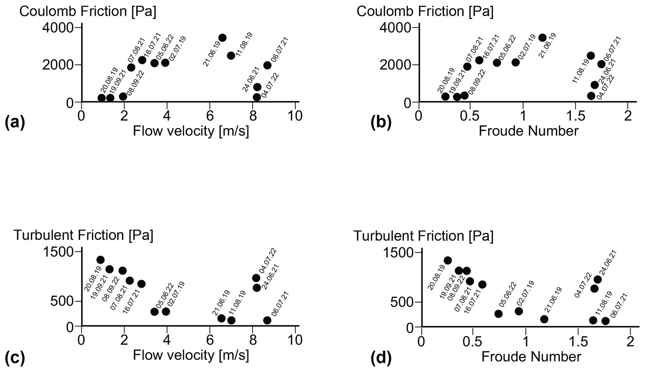
Figure 5 Relationships between (a) flow velocity and Coulomb friction, (b) Froude number and Coulomb friction, (c) flow velocity and turbulent friction, and (d) Froude number and turbulent friction. The plots show the results of the best-fit simulations for each flow.

Figure 6 summarises the consequences of the aforementioned relationships. In particular, small values of the Coulomb friction coefficient (μ ∼ 0.01), when the flow is moving on the order of a few metres per second, indicate that the contribution of the Coulomb term to the total friction is small and that the total friction is therefore dominated by the turbulent friction term (Fig. 6). In the extreme case when μ= 0, the turbulent friction term (Eq. 1) closely resembles a Chézy friction from open-channel hydraulics (e.g. Henderson, 1966). Large values of the Coulomb friction coefficient (here μ ∼ 0.05) suggest that the Coulomb friction term is important and that the contribution of the turbulent friction is correspondingly less significant (Fig. 6). Because we found ideal μ–ξ pairs with μ= 0.01–0.02 and μ = 0.05 for most debris flows, we considered these flows to be dominated by either (i) the turbulent friction (flows with μ= 0.01–0.02) or (ii) the Coulomb friction (flows with μ= 0.05). Note that Fig. 6 also shows that the total friction S increases with a larger μ. Nevertheless, the output of the simulation (velocity and flow depth) is similar regardless of which μ–ξ pair variant is chosen.

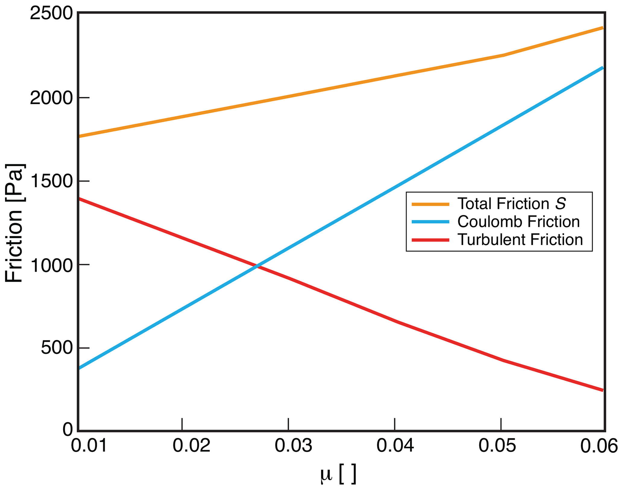
Figure 6 Values of Coulomb friction, turbulent friction, and total friction S as a function of the selected Coulomb friction coefficient μ. The plotted values are averages of the friction magnitudes of all best-fit simulations. The blue line represents the Coulomb friction contribution, the red line is the turbulent friction, and the yellow line is the total friction.

4.3 Grain size distribution

Samples from 14 debris flows were analysed for their grain size distribution (Fig. 7 and Table S6). Note that there was a sediment sample but no monitoring data for the event on 4 October 2021. All events show a very similar grain size distribution. An exception, and thus an outlier, is a sediment sample that has a larger relative abundance of fine-grained material. This sample was taken from a debris flow, which occurred on 2 July 2019. For all samples, the clay fraction has a relative mass abundance of 2 %–3 %, the silt fraction has a relative mass abundance of 27 %–35 %, the sand fraction has a relative mass abundance of 27 %–40 %, and the part of the gravel fraction that is covered by the analysis has a relative mass abundance of 23 %–37 %. Note that the gravel fraction > 16 mm was also analysed (Table S6b). However, we normalised the grain size data to 16 mm, because it was not feasible to collect larger mass-representative samples. Therefore, we acknowledge that the upper percentiles are affected and thus biased by this cutoff and that the related percentage values have to be considered with caution.

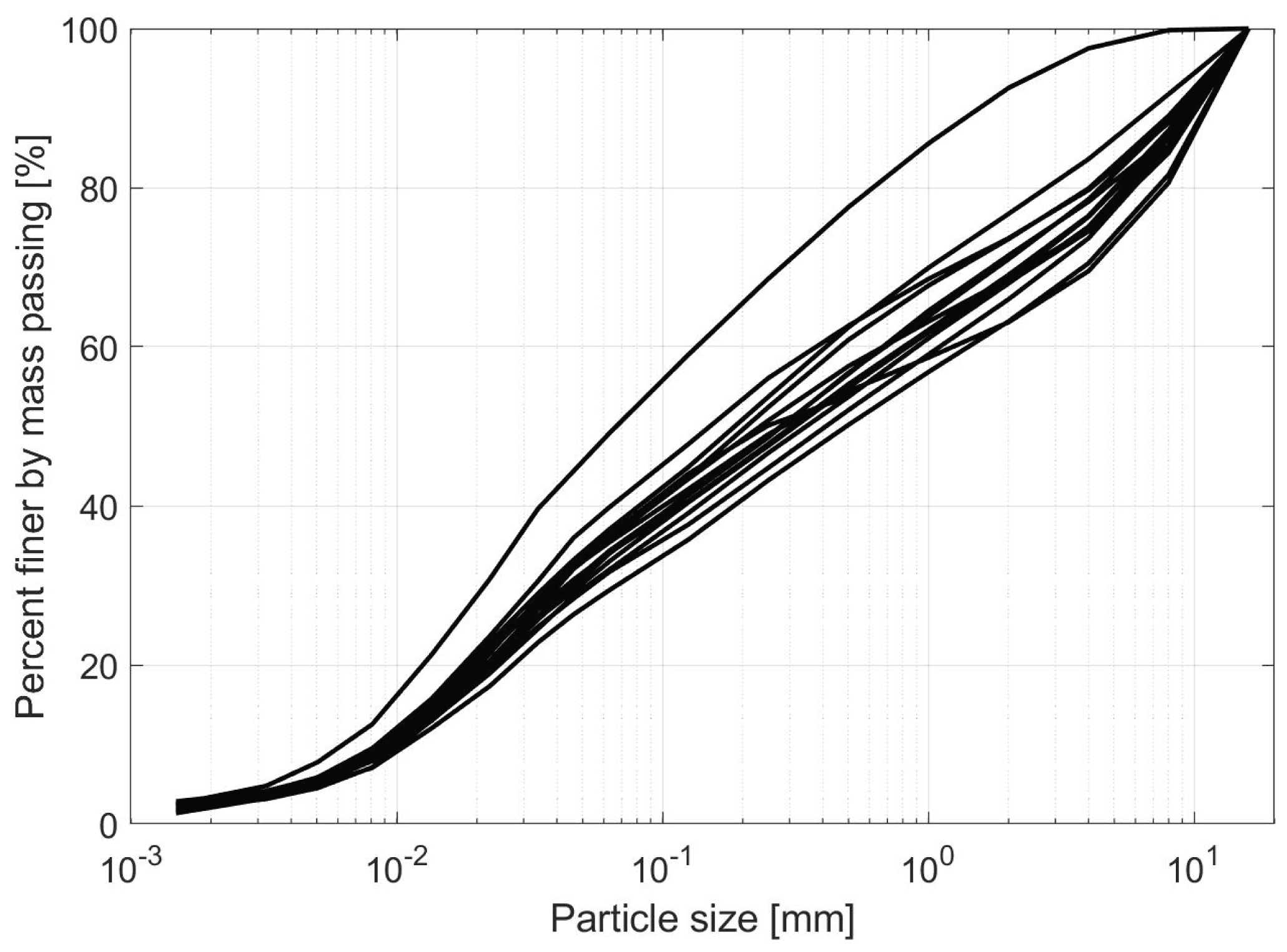
Figure 7 Diagram showing the grain size distribution of all 14 sampled debris flow deposits, truncated at a maximum grain size of 16 mm.

For all samples, we measured grain sizes of 0.015–0.02 mm for the 16th percentile, 4–9 mm for the 84th percentile, and 10–15 mm for the 95th percentile. The median grain size ranges from 0.15 to 0.5 mm. In general, the material was very poorly sorted with a skewness towards the fine-grained fraction. Interestingly, the grain size distribution was quite similar for all of the sampled material. Based on the available datasets, we are neither able to determine whether the mean grain size is more variable in space than in time, nor can we detect whether the coarse-grained fraction (> 16 mm) could be highly variable and the fine-grained material more homogeneous. However, similar to the mineralogical composition, which is also quite similar between the various flows, we interpret that the rather homogeneous granulometric composition, at least of the fine-grained portion of the sediment, is the direct consequence of the cascade of sediment mixing in the upstream part of Illgraben (Schlunegger et al., 2009).

4.4 Powder XRD

The results of the powder XRD analysis (Table S7) show that quartz was the main mineral of the silt fraction and contributed between 29 wt % and 36 wt % (Fig. 8). In addition, dolomite (17 wt %–24 wt %), muscovite (18 wt %–22 wt %), calcite (7 wt %–18 wt %), and illite minerals (8 wt %–12 wt %) are present in all samples. Feldspar grains occur by < 5 wt %, and the clay minerals chlorite, kaolinite, and smectite are present in small quantities (< 1 %) or are below the detection limit. Among the four samples, calcite shows the greatest variation in the mineralogical composition, with differences up to 11 wt %. The other main components including quartz, dolomite, muscovite, and illite show variations of up to a maximum of 7 wt %. The feldspar minerals albite and orthoclase are very homogeneously distributed in the four samples. Overall, the variations in the mineralogical composition between the different samples are only minor and often lie within the methodological error of ±10 % of the measured values. However, some, albeit minor, differences can be detected when the compositions of the coarse- and fine-grained samples are compared. In the coarse-grained sample, calcite crystals are more abundant than in the sample characterising a fine-grained debris flow. In contrast, the latter sample has a larger relative abundance of illite minerals than the sample made up of coarser sediments. Although the database is sparse, we tentatively consider these differences to reflect a source signal where the heavily fractured basement rocks and Triassic schists, which also host the illite crystals, have the potential to supply larger volumes of fine-grained material than the bedrock made up of limestones.

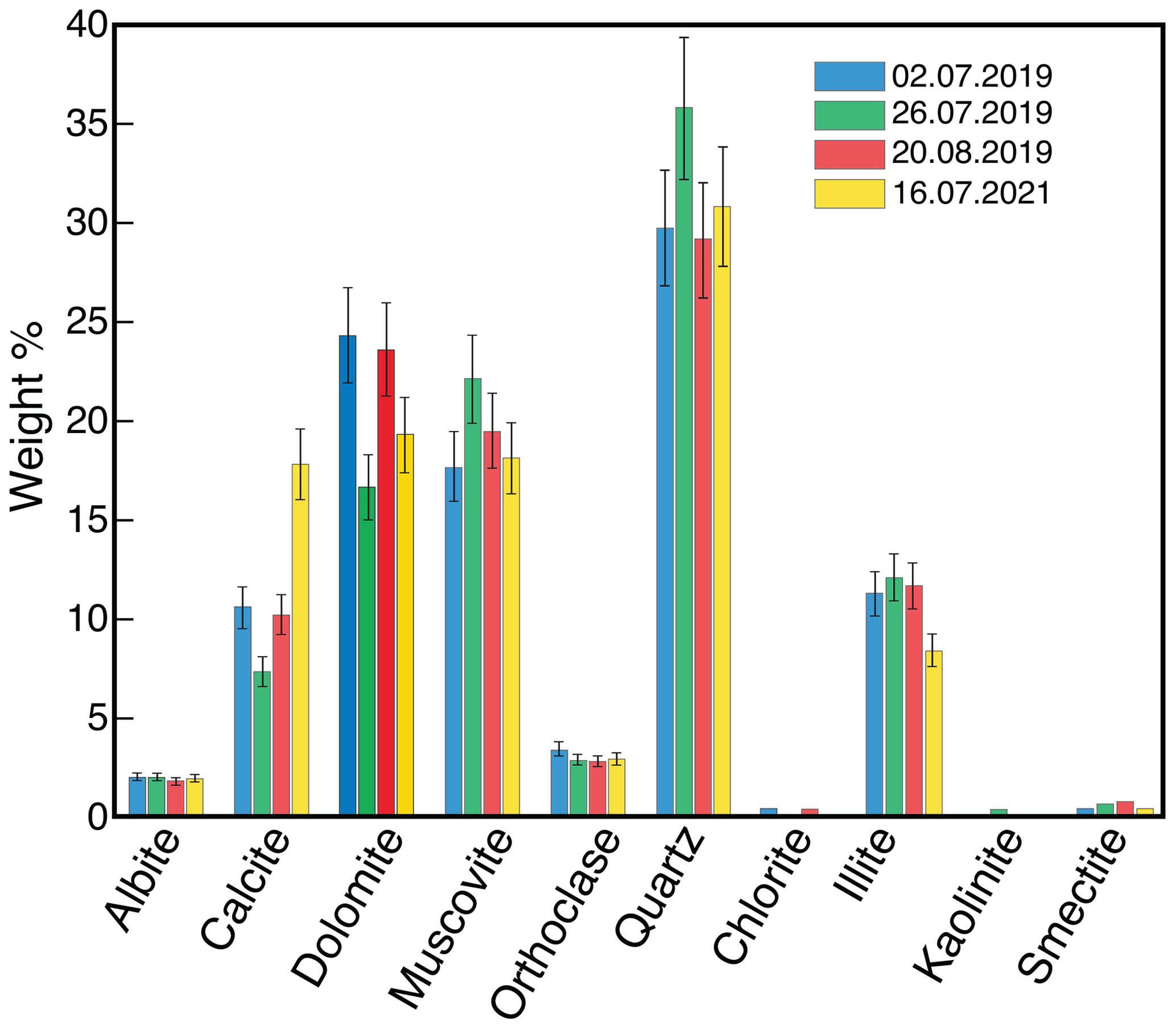
Figure 8 Mineralogic composition of four samples analysed by powder XRD. The black error bars indicate a methodological error of 10 % of the measured value. The material representing the flow on 2 July 2019 was exceptionally fine-grained (Table S6); the flow on 26 July of the same year was an event with a high velocity (8.69 m s⁻¹) and the most rapid flow (Table 1). The debris flow on 20 August, again in 2019, was very slow (0.89 m s⁻¹), and it was indeed the slowest flow during the survey period (Table 1). The material taken from the debris flow on 16 July 2021 was characterised by a rather coarse-grained matrix (Table S6).

From the clay minerals, only smectite can absorb larger amounts of water (Likos and Lu, 2002). However, the X-ray spectra of muscovite and smectite crystals cannot be distinguished between with the applied XRD method. Because the basement rocks and the Triassic schists are considered to be the source of the clay minerals in the catchment area (Schlunegger et al., 2009), the signal is more likely related to the fine-grained muscovite (sericite) than to the smectite minerals (Scheiber et al., 2013). Therefore, swelling clay minerals are expected to be of minor importance in this case.

4.5 Statistical evaluation of the debris flow properties

A statistical evaluation of the debris flow parameters measured at the monitoring station shows a positive correlation between velocity, flow depth, volume, and maximum discharge (Fig. 9). While velocity, volume, and maximum discharge correlate very strongly among themselves as they are physically related (autocorrelation), the correlation of these parameters with the flow depth is less evident, yet a weak positive correlation is certainly visible. Accordingly and as expected (McArdell et al., 2003), a debris flow with a large volume tends to have a large flow velocity and flow depth, which consequently also results in a large maximum discharge and a large Froude number. On the other hand, debris flows that have a small volume are also slow, and they have both a shallow flow depth and a low Froude number. Interestingly, clear correlations between grain size, clay content, and flow properties are not visible in our analyses (Fig. 10). Also, no correlation between the inferred water content and the volume or maximum discharge was found for these events. Yet, the total friction values that are extracted from the modelling results tend to show a positive correlation with the flow depth and a weak positive correlation with the density and thus a weak negative relation to the water content (Fig. 9).

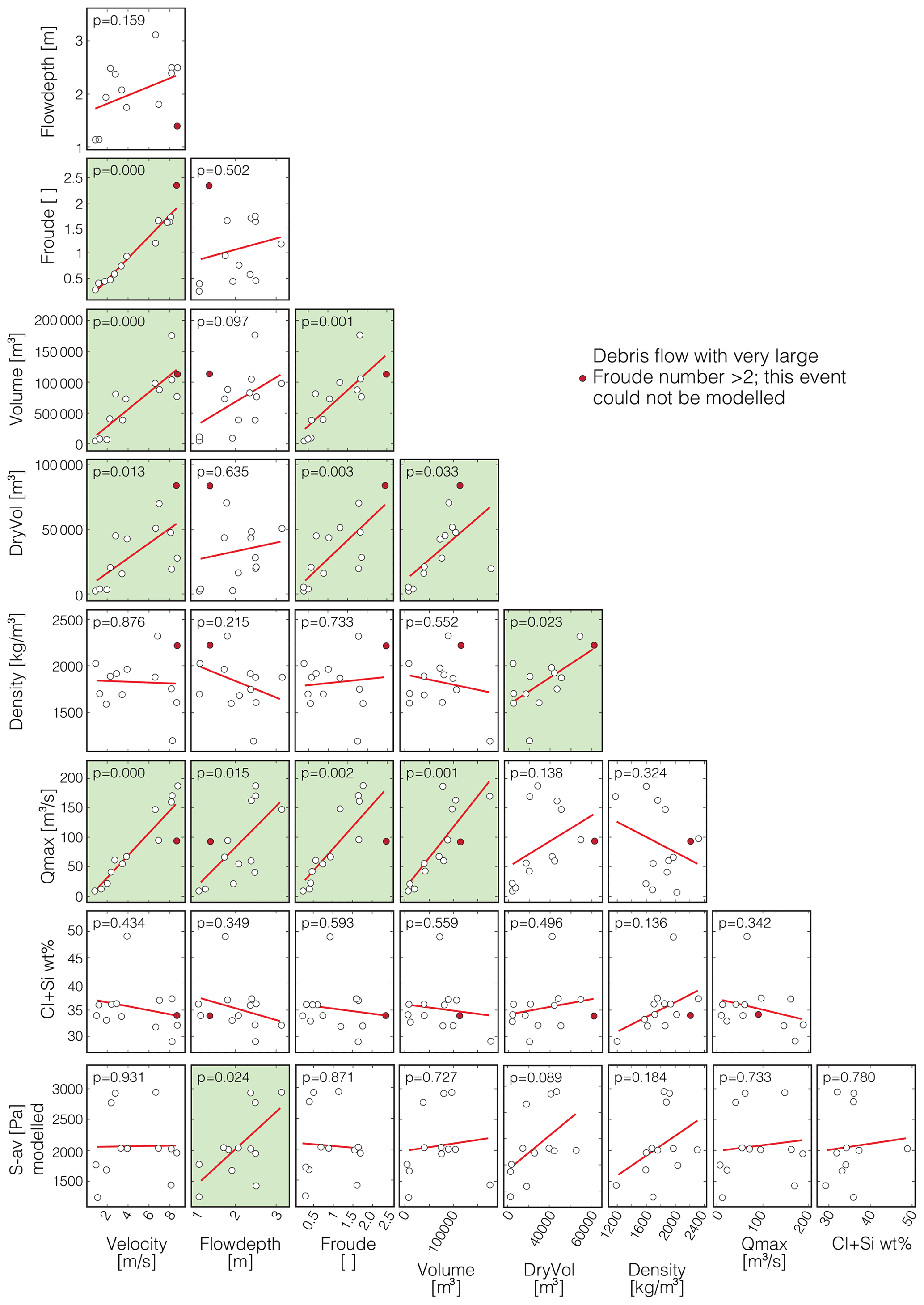
Figure 9 Statistical correlations between the dynamic properties of the debris flows with a statistical p value. For correlation tests, a significance level of 0.05 is considered. Correlations with p values < 0.05 can therefore be considered to be significant (illustrated in green). Measurements from the monitoring station at Illgraben and values derived from them are front velocity [m s⁻¹]; maximum flow depth [m]; Froude number [ ]; total volume [m³]; dry sediment volume [m³]; and density of flow [kg m⁻³], which points to the water content and the maximum discharge [m³ s⁻¹]. From the grain size analyses, we have the percentage of the sum of clay and silt in the sample [wt %]. From the modelling with RAMMS we get the total amount of friction [Pa] as the average of all best-fit simulations of a certain event. The plots were generated using a modified version of the Correlation Matrix Scatterplot graphic created by Chow (2022) for MATLAB. Note that a statistical p value with p= 0.000 means that the value is lower than 0.0005, and therefore it is rounded down to 0.

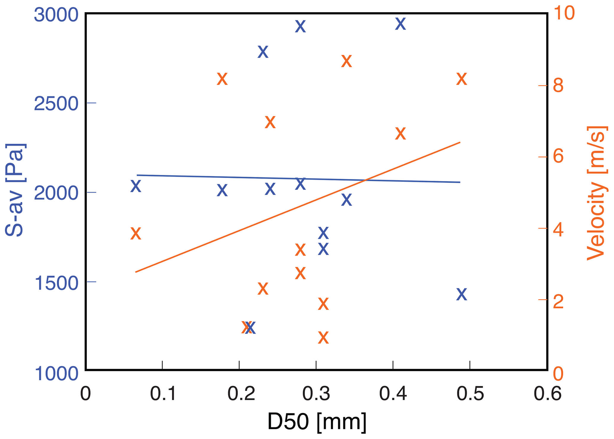
Figure 10 Correlation (first-order polynomial trend lines accomplished by least-squares fitting) between the total amount of friction S-av as the average of all best-fit simulations of a certain event and the D50 value of the corresponding sediment sample (blue) and the correlation between the measured velocity of the flow and the D50 value of the corresponding sediment sample (red).

5 Discussion

The debris flows observed in the years 2019, 2021, and 2022 show large differences in their dynamics, with flow depths and flow velocities varying by a factor of 3 and 10, respectively. Despite these variabilities in the surveyed parameters, most of the flows could be simulated with RAMMS, and the model outputs yielded consistent results regarding the underlying controls and the simulated flow kinematics and properties (see Tables S2, S3, S4, and S5 and the related z values). In the following section, we discuss how the various parameters such as the grain size and mineralogical distribution of the fined-grained matrix as well as the friction properties potentially exerted control over the surveyed debris flows.

5.1 Relationships between volume, flow velocity, and flow depth and controls on friction properties

The statistical tests show positive correlations between volume, flow velocity, flow depth, and maximum discharge rate. Our results are thus consistent with similar results reported by Rickenmann (1999), de Haas et al. (2015), and Hürlimann et al. (2015) and reflect the open-channel hydraulic principles used to compute these parameters (McArdell et al., 2023). Indeed, as shown by the aforementioned authors, flows with larger volumes may contain a larger number of pebbles and boulders, which, according to Johnson et al. (2012), are likely to accumulate at the front of these flows. As a result, the frictional resistance of the frontal part increases (Iverson, 1997), with the consequence of a damming effect such as an increase in flow depths. We indeed see such a mechanism at work in the surveyed flows through positive correlations between flow depth, flow velocity, and flow volume. We thus infer that the volume can be considered to be the most important driving parameter for explaining the debris flow dynamics in the Illgraben system and therefore can be considered to be a key parameter. This confirms the standard practice in hazard analysis, which gives primary importance to event volume. We note that this argument relies on the debris flows all having the same initial grain size distribution, which, as discussed above, we can only document for sediment sizes smaller than 16 mm. However, we acknowledge that a visual comparison of the videos (Fig. S1) clearly shows differences in the abundance of relatively coarse sediment (e.g. boulders). A more detailed analysis on this topic would require additional data and is beyond the scope of this paper.

The evaluation of the RAMMS simulations shows that there are several μ–ξ pairs, which yield ideal solutions upon simulating the surveyed debris flows. In particular, the same flow can successfully be reproduced by RAMMS with high and low Voellmy μ values. However, an assessment of which of these possibilities is more appropriate can be made if the flow velocity is used as a criterion. Indeed, our analysis showed that debris flows with high velocity (up to 6–7 m s⁻¹) tend to be dominated by a large Coulomb friction (large μ value), whereas flows with low velocity have low Coulomb friction (low μ value) but relatively high turbulent friction (Fig. 5). Yet for flows with velocities that are larger than 6–7 m s⁻¹, these relatively simple relationships break down most likely because such flows appear to be in a condition where the flow pattern is more complex (e.g. roll waves with Froude numbers that are much larger than 1 to 1.5; Table 1).

We note that while it is tempting to interpret such low-μ flows as being “laminar” and large-μ flows as “turbulent” (because of the low and high Froude numbers; see also Fig. 5), independent criteria for determining the presence or absence of turbulence in debris flows are not yet available. A hydraulics-based estimate based on the Reynolds number to characterise the presence or absence of turbulence (e.g. Henderson, 1966) requires estimates of the rheology of the entire flow, which are not available. In addition, it is unclear to what extent rheological measurements of fine-sediment slurries can represent the overall viscosity of the flow given the presence of other processes such as the jamming of particles in the flow (Kostynick et al., 2022). However, such calculations are beyond the scope of this contribution.

5.2 Influence of the grain size distribution and mineralogy

The granulometric analysis of the levee deposits indicates a rather homogeneous grain size distribution for the clay, silt, sand, and fine-grained gravel fraction. The grain size distribution fits quite well with the granulometric analyses of the debris flow deposits at Illgraben published by Hürlimann et al. (2003). Because of a lack of correlations between the relative proportion of the fine fraction and the parameters that characterise the flow properties (e.g. friction and flow velocity; Fig. 10), the variations in the dynamics of these flows cannot be simply explained by a simple fixed friction relation such as in the Voellmy relation. This inference is consistent with the notion by Iverson (2003), who states that the evolution of debris flow behaviour upstream of the front is likely to be complex. In the same sense, because of the homogeneity of the samples with respect to the grain size distribution of the components smaller than 16 mm, the relative abundance of the sand and the fine-grained gravel fraction cannot be related to variations in the flow dynamics either. Nevertheless, an influence of the grain size composition on the debris flow dynamics, as described by de Haas et al. (2015) and Hürlimann et al. (2015), cannot be fully excluded (see Sect. 1.1). Because the relative abundances of the different fractions are similar, their potential influence on the flow properties should also be similar for each event. Due to this similarity, such relationships (if present) would not be detectable with the measurements presented herein. Admittedly, we also have no information to exclude a potential control of the coarse-grained fraction such as coarse gravel, cobbles, and boulders on the flow dynamics, as described by de Haas et al. (2015). Attempts to reconstruct the full grain size distribution are hampered by a lack of information on the grain size below the surface of the flow (e.g. Uchida et al., 2021). In addition, the influence of small changes in the topography on the results was not investigated here but could improve the correlations of the flow properties with grain size if adequately considered.

Similar to the grain size distribution of the fine-grained matrix, we do not see a relationship between the mineralogical composition of the matrix and the flow properties. Among the various minerals that are present in the debris flow deposits (Table S7), we expect to see a control of the sheet silicates on the velocity of the flows, mainly because clay minerals and particularly smectite-type clays have the potential to absorb water in their crystal structure (see Sect. 1.1). We therefore expect that a high relative abundance of such minerals will alter the rheology and particularly the turbulent friction of the flows, which is expected to impact the flow velocity. Apparently, this is not the case at Illgraben. We consider this absence of relationships to reflect a supply signal because the relative abundance of swelling minerals is negligible in the source area where other sheet silicates such as illite and muscovite crystals predominate (Scheiber et al., 2013). These silicates do not have swelling properties and apparently do not impact the velocity of the debris flows at Illgraben. However, the homogeneity in terms of the mineral composition and also the grain size composition between the samples confirms the results of previous studies that inferred the occurrence of an efficient mixing mechanism as the material is transferred from the source area to the Rhône River (Schlunegger et al., 2009; Berger et al., 2011a).

6 Conclusions

The results obtained in the Illgraben system by comparing various debris flow parameters with data from runout modelling, grain size analyses, and XRD analyses can be summarised as follows:

1. The simulation of debris flows with RAMMS yields multiple solutions with different friction coefficients μ and ξ in the Voellmy equation. The resulting Coulomb and turbulent frictions are correlated with the Froude number and runout velocity of the debris flow but only as long as the flow velocity is < 6–7 m s⁻¹.

2. The dynamics of a debris flow in Illgraben (i.e. flow velocity and flow depth) is strongly dependent on its volume. If information about the sediment volume in the source area is available, the parameters for simulating a potentially worst-case debris flow and its impact can theoretically be assessed with some uncertainties.

3. Due to the relatively large homogeneity of the deposits with respect to the grain size distribution and the mineralogical composition, an efficient mixing process in Illgraben can be inferred.

4. Based on these data, variations in the dynamics of different debris flows cannot be attributed to the grain size distributions of the clay, silt, sand, or fine-grained gravel fractions. Consequently, an assessment of a potential debris flow or a definition of a simulation based on grain size compositions in the source area is not possible in the case presented here.

Such relationships are particularly useful for the assessment of natural hazards, as they provide specific evidence for the estimation of a debris flow and its impact.